Control of underwater vehicles in inviscid fluids.
I: Irrotational flows.

Abstract.

In this paper, we investigate the controllability of an underwater vehicle immersed in an infinite volume of an inviscid fluid whose flow is assumed to be irrotational. Taking as control input the flow of the fluid through a part of the boundary of the rigid body, we obtain a finite-dimensional system similar to Kirchhoff laws in which the control input appears through both linear terms (with time derivative) and bilinear terms. Applying Coron’s return method, we establish some local controllability results for the position and velocities of the underwater vehicle. Examples with six, four, or only three controls inputs are given for a vehicule with an ellipsoidal shape.

1. Introduction

The control of boats or submarines has attracted the attention of the mathematical community from a long time (see e.g. [2, 3, 4, 9, 10, 16, 17, 18, 19].) In most of the papers devoted to that issue, the fluid is assumed to be inviscid, incompressible and irrotational, and the rigid body (the vehicle) is supposed to have an elliptic shape. On the other hand, to simplify the model, the control is often assumed to appear in a linear way in a finite-dimensional system describing the dynamics of the rigid body, the so-called Kirchhoff laws.

A large vessel (e.g. a cargo ship) presents often one tunnel thruster built into the bow to make docking easier. Some accurate model of a boat without rudder controlled by two propellers, the one displayed in a transversal bowthruster at the bow of the ship, the other one placed at the stern of the boat, was derived and investigated in [12]. A local controllability result for the position and velocity (six coordinates) of a boat surrounded by an inviscid (not necessarily irrotational) fluid was derived in [12] with only two controls inputs.

The aim of this paper is to provide some accurate model of a neutrally buoyant underwater vehicle immersed in an infinite volume of ideal fluid, without rudder, and actuated by a few number of propellers located into some tunnels inside the rigid body, and to give a rigorous analysis of the control properties of such a system. We aim to control both the position, the attitude, and the (linear and angular) velocities of the vehicle by taking as control input the flow of the fluid through a part of the boundary of the rigid body. The inviscid incompressible fluid is assumed here to have an irrotational (hence potential) flow, for the sake of simplicity. The case of a fluid with vorticity will be considered elsewhere.

Our fluid-structure interaction problem can be described as follow. The underwater vehicle, represented by a rigid body occupying a connected compact set $\mathcal{S}(t)\subset\mathbb{R}^{3}$, is surrounded by an homogeneous incompressible perfect fluid filling the open set $\Omega(t):=\mathbb{R}^{3}\setminus\mathcal{S}(t)$ (as e.g. for a submarine immersed in an ocean). We assume that $\Omega(t)$ is $C^{\infty}$ smooth and connected. Let $\mathcal{S}=\mathcal{S}(0)$ and

$$\Omega=\Omega(0)=\mathbb{R}^{3}\setminus\mathcal{S}(0)$$

denote the initial configuration ($t=0$). Then, the dynamics of the fluid-structure system are governed by the following system of PDE’s

$$\displaystyle\frac{\partial u}{\partial t}+(u\cdot\nabla)u+\nabla p=0, t\in(0,T),\;x\in\Omega(t),\qquad$$ (1.1)

$$\textrm{div }u=0, t\in(0,T),\;x\in\Omega(t),\qquad$$ (1.2)

$$u\cdot\nu=(h^{\prime}+\omega\times(x-h))\cdot\nu+w(t,x), t\in(0,T),\;x\in\partial\Omega(t),\qquad$$ (1.3)

$$\lim\limits_{|x|\to+\infty}u(t,x)=0, t\in(0,T),$$ (1.4)

$$m_{0}h^{\prime\prime}=\displaystyle\int\limits_{\partial\Omega(t)}p\nu\,d\sigma, t\in(0,T),$$ (1.5)

$$\displaystyle\frac{d}{dt}(QJ_{0}Q^{\ast}\omega)=\displaystyle\int\limits_{\partial\Omega(t)}(x-h)\times p\nu\,d\sigma, t\in(0,T),$$ (1.6)

$$Q^{\prime}=S(\omega)Q, t\in(0,T),$$ (1.7)

$$u(0,x)=u_{0}(x), x\in\Omega,$$ (1.8)

$$(h(0),Q(0),h^{\prime}(0),\omega(0))=(h_{0},Q_{0},h_{1},\omega_{0}) \in \mathbb{R}^{3}\times\text{SO}(3)\times\mathbb{R}^{3}\times\mathbb{R}^{3}.$$ (1.9)

In the above equations, $u$ (resp. $p$) is the velocity field (resp. the pressure) of the fluid, $h$ denotes the position of the center of mass of the solid, $\omega$ denotes the angular velocity and $Q$ the 3 dimensional rotation matrix giving the orientation of the solid. The positive constant $m_{0}$ and the matrix $J_{0}$, which denote respectively the mass and the inertia matrix of the rigid body, are defined as

$$m_{0}=\int\limits_{\mathcal{S}}\rho(x)dx,\;\;\;J_{0}=\displaystyle\int\limits_{\mathcal{S}}\rho(x)(|x|^{2}Id-xx^{\ast})dx,$$

where $\rho(\cdot)$ represents the density of the rigid body. Finally, $\nu$ is the outward unit vector to $\partial\Omega(t)$, $x\times y$ is the cross product between the vectors $x$ and $y$, and $S(y)$ is the skew-adjoint matrix such that $S(y)x=y\times x$, i.e.

$$S(y)=\left(\begin{array}[]{ccc}0&-y_{3}&y_{2}\\ y_{3}&0&-y_{1}\\ -y_{2}&y_{1}&0\end{array}\right).$$

The neutral buoyancy condition reads

$$\int\limits_{\mathcal{S}}\rho(x)dx=\int\limits_{\mathcal{S}}1dx.$$ (1.10)

$f^{\prime}$ (or $\dot{f}$) stands for the derivative of $f$ respect to $t$, $A^{\ast}$ means the transpose of the matrix $A$, and $Id$ denotes the identity matrix. Finally, the term $w(t,x)$, which stands for the flow through the boundary of the rigid body, is taken as control input. Its support will be strictly included in $\partial\Omega(t)$, and actually only a finite dimensional control input will be considered here (see below (1.17) for the precise form of the control term $w(t,x)$).

When no control is applied (i.e. $w(t,x)=0$), then the existence and uniqueness of strong solutions to (1.1)-(1.9) was obtained first in [20] for a ball embedded in $\mathbb{R}^{2}$, and next in [21] for a rigid body $\mathcal{S}$ of arbitrary form (still in $\mathbb{R}^{2}$). The case of a ball in $\mathbb{R}^{3}$ was investigated in [22], and the case of a rigid body of arbitrary form in $\mathbb{R}^{3}$ was studied in [25]. The detection of the rigid body $\mathcal{S}(t)$ from partial measurements of the fluid velocity has been tackled in [5] when $\Omega(t)=\Omega_{0}\setminus\overline{\mathcal{S}(t)}$ ($\Omega_{0}\subset\mathbb{R}^{2}$ being a bounded cavity) and in [6] when $\Omega(t)=\mathbb{R}^{2}\setminus\overline{\mathcal{S}(t})$.

Here, we are interested in the control properties of (1.1)-(1.9). The controllability of Euler equations has been established in 2D (resp. in 3D) in [7] (resp. in [11]). Note, however, that there is no hope here to control the motion of both the fluid and the rigid body. Indeed, $\Omega(t)$ is an exterior domain, and the vorticity is transported by the flow with a finite speed propagation, so that it is not affected (at any given time) far from the rigid body. Therefore, we will deal with the control of the motion of the rigid body only. As the state of the rigid body is described by a vector in $\mathbb{R}^{12}$, it is natural to consider a finite-dimensional control input.

Note also that since the fluid is flowing through a part of the boundary of the rigid body, additional boundary conditions are needed to ensure the uniqueness of the solution of (1.1)-(1.9) (see [13], [14]). In dimension three, one can specify the tangent components of the vorticity $\zeta(t,x):=\textrm{curl }v(t,x)$ on the inflow section; that is, one can set

$$\zeta(t,x)\cdot\tau_{i}=\zeta_{0}(t,x)\cdot\tau_{i}\;\;\textrm{for }w(t,x)<0,\ i=1,2,$$ (1.11)

where $\zeta_{0}(t,x)$ is a given function and $\tau_{i}$, $i=1,2$, are linearly independent vectors tangent to $\partial\Omega(t)$. As we are concerned here with irrotational flows, we choose $\zeta_{0}\equiv 0$.

In order to write the equations of the fluid in a fixed frame, we perform a change of coordinates. We set

$$x = Q(t)y+h(t),$$ (1.12)

$$v(t,y) = Q^{\ast}(t)u(t,Q(t)y+h(t)),$$ (1.13)

$$q(t,y) = p(t,Q(t)y+h(t)),$$ (1.14)

$$l(t) = Q^{\ast}(t)h^{\prime}(t),$$ (1.15)

$$r(t) = Q^{\ast}(t)\omega(t).$$ (1.16)

Then $x$ (resp. $y$) represents the vector of coordinates of a point in a fixed frame (respectively in a frame linked to the rigid body). We may without loss of generality assume that

$$h(0)=0,\qquad Q(0)=Id.$$

Note that, at any given time $t$, $y$ ranges over the fixed domain $\Omega$ when $x$ ranges over $\Omega(t)$. Finally, we assume that the control takes the form

$$w(t,x)=w(t,Q(t)y+h(t))=\sum_{j=1}^{m}w_{j}(t)\chi_{j}(y),$$ (1.17)

where $m\in\mathbb{N}^{\ast}$ stands for the number of independent inputs, and $w_{j}(t)\in\mathbb{R}$ is the control input associated with the function $\chi_{j}\in C^{\infty}(\partial\Omega)$. To ensure the conservation of the mass of the fluid, we impose the relation

$$\int\limits_{\partial\Omega}\chi_{j}(y)d\sigma=0\;\textrm{ for }1\leq j\leq m.$$ (1.18)

Then the functions $(v,q,l,r)$ satisfy the following system

$$\displaystyle\frac{\partial v}{\partial t}+((v-l-r\times y)\cdot\nabla)v+r\times v+\nabla q=0, t\in(0,T),\;y\in\Omega,$$ (1.19)

$$\textrm{div }v=0, t\in(0,T),\;y\in\Omega,$$ (1.20)

$$\displaystyle v\cdot\nu=(l+r\times y)\cdot\nu+\sum\limits_{1\leq j\leq m}w_{j}(t)\chi_{j}(y), t\in(0,T),\;y\in\partial\Omega,$$ (1.21)

$$\lim\limits_{|y|\to+\infty}v(t,y)=0, t\in(0,T),$$ (1.22)

$$m_{0}\dot{l}=\displaystyle\int\limits_{\partial\Omega}q\nu\,d\sigma-m_{0}r\times l, t\in(0,T),$$ (1.23)

$$J_{0}\dot{r}=\displaystyle\int\limits_{\partial\Omega}q(y\times\nu)\,d\sigma-r\times J_{0}r, t\in(0,T),$$ (1.24)

$$(l(0),r(0))=(h_{1},\omega_{0}),\;v(0,y)=u_{0}(y).$$ (1.25)

The paper is organized as follows. In Section 2, we simplify system (1.1)-(1.9) by assuming that the fluid is potential. We obtain a finite dimensional system (namely (2.65)) similar to Kirchhoff laws, in which the control input $w$ appears through both linear terms (with time derivative) and bilinear terms. The investigation of the control properties of (2.65) is performed in Section 3. After noticing that the controllability of the linearized system at the origin requires six control inputs, we apply the return method due to Jean-Michel Coron to take advantage of the nonlinear terms in (2.65). (We refer the reader to [8] for an exposition of that method for finite-dimensional systems and for PDE’s.) We consider the linearization along a certain closed-loop trajectory and obtain a local controllability result (Theorem 3.11) assuming that two rank conditions are fulfilled, by using a variant of Silverman-Meadows test for the controllability of a time-varying linear system. Some examples using symmetry properties of the rigid body are given in Section 4.

2. Equations of the motion in the potential case

In this section we derive the equations describing the motion of the rigid body subject to flow boundary control when the fluid is potential.

2.1. Null vorticity

Let us denote by

$$\zeta(t,y)=\textrm{curl}\,v(t,y):=(\nabla\times v)(t,y)$$

the vorticity of the fluid. Here, we assume that

$$\zeta_{0}=\textrm{curl}\,v_{0}=0\;\;\;\textrm{ in }\Omega$$ (2.1)

and that the three components of $\zeta$ are null at the inflow part of $\partial\Omega$, namely

$$\zeta(t,y)=0,\;\;\;\textrm{if }\;y\in\cup_{1\leq j\leq m}\text{ Supp }\chi_{j}\ \text{ and }\ \sum_{j=1}^{m}w_{j}(t)\chi_{j}(y)\leq 0.$$ (2.2)

Proposition 2.1.

Under the assumptions (2.1) and (2.2), one has

$$\zeta=\textrm{\rm curl}\,v\equiv 0\;\;\textrm{ in }[0,T]\times\Omega,$$ (2.3)

Proof.

Let us introduce $\tilde{v}:=v-l-r\times y$. Then it follows from (1.20) that

$$\textrm{div}(\tilde{v})=0,$$ (2.4)

and

$$\textrm{curl}(\tilde{v})=\zeta-2r.$$ (2.5)

Applying the operator curl in (1.19) results in

$$\frac{\partial\zeta}{\partial t}+\textrm{curl}((\tilde{v}\cdot\nabla)\tilde{v})+\textrm{curl}((\tilde{v}\cdot\nabla)(l+r\times y))+\textrm{curl}(r\times v)=0.$$ (2.6)

We note that the following identities hold:

$$\textrm{curl}((v\cdot\nabla)v)=(v\cdot\nabla)\textrm{curl}(v)-(\textrm{curl}(v)\cdot\nabla)v+\textrm{div}(v)\textrm{curl}(v)$$ (2.7)

and

$$(v\cdot\nabla)(r\times y)=r\times v,\;\;\;\textrm{curl}(r\times v)=\textrm{div}(v)r-(r\cdot\nabla)v.$$ (2.8)

Using (2.4)-(2.8), we see that $\zeta$ satisfies

$$\frac{\partial\zeta}{\partial t}+(\tilde{v}\cdot\nabla)\zeta-(\zeta\cdot\nabla)\tilde{v}=0.$$ (2.9)

Let $\varphi=\varphi(t,s,y)$ denote the flow associated with $\tilde{v}$, i.e.

$$\frac{\partial\varphi}{\partial t}=\tilde{v}(t,\varphi),\;\textrm{with}\;\varphi{|_{t=s}}=y.$$ (2.10)

We denote by $G(t,s,y)=\frac{\partial\varphi}{\partial y}(t,s,y)$ the Jacobi matrix of $\varphi$. Differentiating in (2.10) with respect to $y_{j}$ ($j=1,2,3$), we see that $G(t,s,y)$ satisfies the following equation:

$$\frac{\partial G}{\partial t}=\displaystyle\frac{\partial\tilde{v}}{\partial y}(t,\varphi(t,s,y))\cdot G(t,s,y),\;\textrm{where}\;\;G(s,s,y)=Id\;\textrm{(identity matrix)}.$$ (2.11)

We infer from (2.4) and (2.11) that

$$\textrm{det }G(t,s,y)=1.$$ (2.12)

Following Yudovich [13], we introduce the time $t^{\ast}(t,y)\in[0,t]$ at which the fluid element first appears in $\overline{\Omega}$, and set $y^{\ast}(t,y)=\varphi(t^{\ast}(t,y),t,y)$. Then either $t^{\ast}=0$, or $t^{\ast}>0$ and $y^{\ast}\in\cup_{1\leq j\leq m}\textrm{ supp }\chi_{j}\subset\partial\Omega$ with $\sum_{j=1}^{m}w_{j}(t^{\ast})\chi_{j}(y^{\ast})\leq 0$. Set $f(s,t,y)=G^{-1}(s,t,y)\zeta(s,\varphi(s,t,y))$. From (2.9)-(2.12), we obtain that

$$\frac{\partial f}{\partial s}(s,t,y)=0.$$ (2.13)

Finally, integrating with respect to $s$ in (2.13) yields

$$\zeta(t,y)=G^{-1}(t^{\ast},t,y)\zeta(t^{\ast},y^{\ast}),$$ (2.14)

which, combined to (2.1) and (2.2), gives (2.3). The proof of Proposition 2.1 is complete. ∎

Remark 2.2.

The issue whether the result in Proposition 2.1 still holds with (2.2) replaced by

$$\zeta(t,y)\cdot\tau_{i}=0,\ i=1,2,\;\;\;\textrm{if }\;y\in\cup_{1\leq j\leq m}\text{ Supp }\chi_{j}\ \text{ and }\ \sum_{j=1}^{m}w_{j}(t)\chi_{j}(y)\leq 0,$$

seems challenging. We notice that the result in [14] was proved solely when $\Omega$ was a cylinder.

2.2. Decomposition of the fluid velocity

It follows from (1.20), (1.22) and (2.3) that the flow is potential; that is,

$$v=\nabla\Phi,$$ (2.15)

where $\Phi=\Phi(t,y)$ solves

$$\Delta\Phi=0,\;\;\;\textrm{in }(0,T)\times\Omega,$$ (2.16)

$$\frac{\partial\Phi}{\partial\nu}=(l+r\times y)\cdot\nu+\sum\limits_{1\leq j\leq m}w_{j}(t)\chi_{j}(y)\;\;\;\textrm{on }(0,T)\times\Omega,$$ (2.17)

$$\lim\limits_{|y|\to+\infty}\nabla\Phi(t,y)=0,\;\;\;\textrm{on }(0,T).$$ (2.18)

Actually, $\Phi$ may be decomposed as

$$\Phi(t,y)=\sum\limits_{1\leq i\leq 3}\big{\{}l_{i}\phi_{i}+r_{i}\varphi_{i}\big{\}}+\sum\limits_{1\leq j\leq m}w_{j}\psi_{j}$$ (2.19)

where, for $i=1,2,3$ and $j=1,...,m$,

$$\Delta\phi_{i}=\Delta\varphi_{i}=\Delta\psi_{j}=0\textrm{ in }\Omega,$$ (2.20)

$$\frac{\partial\phi_{i}}{\partial\nu}=\nu_{i},\;\;\displaystyle\frac{\partial\varphi_{i}}{\partial\nu}=(y\times\nu)_{i},\;\;\displaystyle\frac{\partial\psi_{j}}{\partial\nu}=\chi_{j}\textrm{ on }\partial\Omega,$$ (2.21)

$$\lim\limits_{|y|\to+\infty}\nabla\phi_{i}(y)=0,\;\;\displaystyle\lim\limits_{|y|\to+\infty}\nabla\varphi_{i}(y)=0,\;\;\displaystyle\lim\limits_{|y|\to+\infty}\nabla\psi_{j}(y)=0.$$ (2.22)

As the open set $\Omega$ and the functions $\chi_{j}$, $1\leq j\leq m$, supporting the control are assumed to be smooth, we infer that the functions $\nabla\phi_{i}$ ($i=1,2,3$), the functions $\nabla\varphi_{i}$ ($i=1,2,3$) and the functions $\nabla\psi_{j}$ ($1\leq j\leq m$) belong to $H^{\infty}(\Omega)$.

2.3. Equations for the linear and angular velocities

For notational convenience, in what follows $\int_{\Omega}f$ (resp. $\int_{\partial\Omega}f$) stands for $\int_{\Omega}f(y)dy$ (resp. $\int_{\partial\Omega}f(y)d\sigma(y)$).

Let us introduce the matrices $M,J,N\in\mathbb{R}^{3\times 3}$, $C^{M},C^{J}\in\mathbb{R}^{3\times m}$, $L^{M}_{p},L^{J}_{p},R^{M}_{p},R^{J}_{p}\in\mathbb{R}^{3\times 3}$, and the matrices $W^{M}_{p},W^{J}_{p}\in\mathbb{R}^{3\times m}$ for $p\in\{1,...,m\}$ defined by

$$M_{i,j}=\int\limits_{\Omega}\nabla\phi_{i}\cdot\nabla\phi_{j}=\int\limits_{\partial\Omega}\nu_{i}\phi_{j}=\int\limits_{\partial\Omega}\frac{\partial\phi_{i}}{\partial\nu}\phi_{j},$$ (2.23)

$$J_{i,j}=\int\limits_{\Omega}\nabla\varphi_{i}\cdot\nabla\varphi_{j}=\int\limits_{\partial\Omega}(y\times\nu)_{i}\varphi_{j}=\int\limits_{\partial\Omega}\frac{\partial\varphi_{i}}{\partial\nu}\varphi_{j},$$ (2.24)

$$N_{i,j}=\int\limits_{\Omega}\nabla\phi_{i}\cdot\nabla\varphi_{j}=\int\limits_{\partial\Omega}\nu_{i}\varphi_{j}=\int\limits_{\partial\Omega}\phi_{i}(y\times\nu)_{j},$$ (2.25)

$$(C^{M})_{i,j}=\int\limits_{\Omega}\nabla\phi_{i}\cdot\nabla\psi_{j}=\int\limits_{\partial\Omega}\nu_{i}\psi_{j}=\int\limits_{\partial\Omega}\phi_{i}\chi_{j},$$ (2.26)

$$(C^{J})_{i,j}=\int\limits_{\Omega}\nabla\varphi_{i}\cdot\nabla\psi_{j}=\int\limits_{\partial\Omega}(y\times\nu)_{i}\psi_{j}=\int\limits_{\partial\Omega}\varphi_{i}\chi_{j},$$ (2.27)

$$(L^{M}_{p})_{i,j}=\displaystyle\int\limits_{\partial\Omega}(\nabla\phi_{j})_{i}\chi_{p}, (L^{J}_{p})_{i,j}=\displaystyle\int\limits_{\partial\Omega}(y\times\nabla\phi_{j})_{i}\chi_{p},$$ (2.28)

$$(R^{M}_{p})_{i,j}=\displaystyle\int\limits_{\partial\Omega}(\nabla\varphi_{j})_{i}\chi_{p}, (R^{J}_{p})_{i,j}=\displaystyle\int\limits_{\partial\Omega}(y\times\nabla\varphi_{j})_{i}\chi_{p},$$ (2.29)

$$(W^{M}_{p})_{i,j}=\displaystyle\int\limits_{\partial\Omega}(\nabla\psi_{j})_{i}\chi_{p}, (W^{J}_{p})_{i,j}=\displaystyle\int\limits_{\partial\Omega}(y\times\nabla\psi_{j})_{i}\chi_{p}.$$ (2.30)

Note that $M^{\ast}=M$ and $J^{\ast}=J.$

Let us now reformulate the equations for the motion of the rigid body. We define the matrix $\mathcal{J}\in\mathbb{R}^{6\times 6}$ by

$$\mathcal{J}=\left(\begin{array}[]{cc}m_{0}\,Id&0\\ 0&J_{0}\end{array}\right)+\left(\begin{array}[]{cc}M&N\\ N^{\ast}&J\end{array}\right).$$ (2.31)

It is easy to see that $\mathcal{J}$ is a (symmetric) positive definite matrix. We associate to the (linear and angular) velocity $(l,r)\in\mathbb{R}^{3}\times\mathbb{R}^{3}$ of the rigid body a momentum-like quantity, the so-called impulse $(P,\Pi)\in\mathbb{R}^{3}\times\mathbb{R}^{3}$, defined by

$$\mathcal{J}\left(\begin{array}[]{c}l\\ r\end{array}\right)=\left(\begin{array}[]{c}P\\ \Pi\end{array}\right).$$ (2.32)

We are now in a position to give the equations governing the dynamics of the impulse.

Proposition 2.3.

The dynamics of the system are governed by the following Kirchhoff equations

$$\begin{array}[]{rcl}\displaystyle\frac{dP}{dt}+C^{M}\dot{w}&=&\displaystyle(P+C^{M}w)\times r-\sum\limits_{1\leq p\leq m}w_{p}\left\{L^{M}_{p}l+R^{M}_{p}r+W^{M}_{p}w\right\},\\ \\ \displaystyle\frac{d\Pi}{dt}+C^{J}\dot{w}&=&\displaystyle(\Pi+C^{J}w)\times r+(P+C^{M}w)\times l-\sum\limits_{1\leq p\leq m}w_{p}\left\{L^{J}_{p}l+R^{J}_{p}r+W^{J}_{p}w\right\},\end{array}$$ (2.33)

where $w(t):=(w_{1}(t),...,w_{m}(t))\in\mathbb{R}^{m}$ denotes the control input.

Proof.

We first express the pressure $q$ in terms of $l,r,v$ and their derivatives. Using (2.3), we easily obtain

$$v\cdot\nabla v=\nabla\frac{|v|^{2}}{2}\;\;\;\textrm{and}\;\;\;(r\times y)\cdot\nabla v-r\times v=\nabla((r\times y)\cdot v)$$ (2.34)

Thus (1.19) gives

$$\begin{array}[]{lcl}\displaystyle-\nabla q&=&\displaystyle\frac{\partial v}{\partial t}+\nabla\left(\frac{|v|^{2}}{2}-l\cdot v-(r\times y)\cdot v\right)\\ \\ &=&\displaystyle\nabla\left(\sum\limits_{1\leq i\leq 3}\big{\{}\dot{l}_{i}\phi_{i}+\dot{r}_{i}\varphi_{i}\big{\}}+\sum\limits_{1\leq j\leq m}\dot{w}_{j}\psi_{j}+\frac{|v|^{2}}{2}-l\cdot v-(r\times y)\cdot v\right)\end{array}$$

hence we can take

$$q=-\bigg{\{}\sum\limits_{1\leq i\leq 3}\big{\{}\dot{l}_{i}\phi_{i}+\dot{r}_{i}\varphi_{i}\big{\}}+\sum\limits_{1\leq j\leq m}\dot{w}_{j}\psi_{j}+\frac{|v|^{2}}{2}-\left(l+(r\times y)\right)\cdot v\bigg{\}}$$ (2.35)

Replacing $q$ by its value in (1.23) yields

$$m_{0}\dot{l}=-m_{0}r\times l-\bigg{\{}\sum\limits_{1\leq i\leq 3}\bigg{(}\dot{l}_{i}\int\limits_{\partial\Omega}\phi_{i}\nu+\dot{r}_{i}\int\limits_{\partial\Omega}\varphi_{i}\nu\bigg{)}+\sum\limits_{1\leq j\leq m}\dot{w}_{j}\int\limits_{\partial\Omega}\psi_{j}\nu+\int\limits_{\partial\Omega}\left(\frac{|v|^{2}}{2}-\left(l+(r\times y)\right)\cdot v\right)\nu\bigg{\}}.$$ (2.36)

Using (2.34) and (1.20)-(1.21), we obtain

$$\displaystyle\int_{\partial\Omega}{\frac{|v|^{2}}{2}\nu} = \displaystyle\int\limits_{\Omega}\nabla\frac{|v|^{2}}{2}$$ (2.37)

$$= \displaystyle\int\limits_{\Omega}v\cdot\nabla v$$

$$= \displaystyle-\int\limits_{\Omega}(\textrm{div}\,v)v+\int\limits_{\partial\Omega}(v\cdot\nu)v$$

$$= \displaystyle\int\limits_{\partial\Omega}\left((l+r\times y)\cdot\nu\right)v+\sum\limits_{1\leq j\leq m}w_{j}(t)\int\limits_{\partial\Omega}\chi_{j}(y)v.$$

Using Lagrange’s formula:

$$a\times(b\times c)=(a\cdot c)b-(a\cdot b)c,\;\;\forall a,b,c\in\mathbb{R}^{3},$$ (2.38)

we obtain that

$$\int\limits_{\partial\Omega}\left((l+r\times y)\cdot\nu\right)v-\left(\left(l+r\times y\right)\cdot v\right)\nu=\int\limits_{\partial\Omega}(l+r\times y)\times(v\times\nu).$$ (2.39)

Now we claim that

$$\int\limits_{\partial\Omega}\nu\times\nabla f=0,\;\;\;\forall f\in C^{2}(\overline{\Omega}).$$ (2.40)

To prove the claim, we introduce a smooth cutoff function $\rho_{a}$ such that

$$\rho_{a}(y)=\left\{\begin{array}[]{ll}1&\text{if }\ |y|<a,\\ 0&\text{if }\ |y|>2a.\end{array}\right.$$

Pick a radius $a>0$ such that $\mathcal{S}\subset B(0,a)$, and set

$$\tilde{f}(y)=f(y)\rho_{a}(y).$$ (2.41)

Then

$$\nabla\tilde{f}(y)=\nabla f(y),\;\;\forall y\in\partial\Omega,$$

and using the divergence theorem, we obtain

$$\int\limits_{\partial\Omega}\nu\times\nabla f=\int\limits_{\partial\Omega}\nu\times\nabla\tilde{f}=\int\limits_{\Omega}\textrm{curl}(\nabla\tilde{f})=0.$$

Therefore, using (2.40) with $f=\Phi$ where $\nabla\Phi=v$, we obtain

$$\int\limits_{\partial\Omega}l\times(v\times\nu)=0.$$ (2.42)

Another application of (2.40) with $f=y_{i}\Phi$ yields

$$\int\limits_{\partial\Omega}y_{i}v\times\nu=\int\limits_{\partial\Omega}\nu\times e_{i}\Phi,$$ (2.43)

where $\{e_{1},e_{2},e_{3}\}$ denotes the canonical basis in $\mathbb{R}^{3}$. It follows from (2.42), (2.43), and (2.38) that

$$\int\limits_{\partial\Omega}(l+r\times y)\times(v\times\nu)=\displaystyle r\times\int\limits_{\partial\Omega}\Phi\nu\\ =\displaystyle r(t)\times\bigg{(}\sum_{i=1}^{3}\Big{\{}l_{i}(t)\int\limits_{\partial\Omega}\phi_{i}(y)\nu(y)+r_{i}(t)\int\limits_{\partial\Omega}\varphi_{i}(y)\nu(y)\Big{\}}+\sum_{j=1}^{m}w_{j}(t)\int\limits_{\partial\Omega}\psi_{j}(y)\nu(y)\bigg{)}.$$ (2.44)

Combining (2.36) with (2.37), (2.39), and (2.44) yelds

$$m_{0}\dot{l} = \displaystyle-\left\{\sum_{i=1}^{3}\dot{l}_{i}\int\limits_{\partial\Omega}\phi_{i}\nu+\dot{r}_{i}\int\limits_{\partial\Omega}\varphi_{i}\nu+\sum_{j=1}^{m}\dot{w}_{j}\int\limits_{\partial\Omega}\psi_{j}\nu\right\}$$ (2.45)

$$\displaystyle-\sum_{j=1}^{m}w_{j}\left\{\sum_{i=1}^{3}l_{i}\int\limits_{\partial\Omega}\chi_{j}\nabla\phi_{i}+r_{i}\int\limits_{\partial\Omega}\chi_{j}\nabla\varphi_{i}+\sum_{p=1}^{m}w_{p}\int\limits_{\partial\Omega}\chi_{j}\nabla\psi_{p}\right\}$$

$$\displaystyle-r\times\left\{\sum_{i=1}^{3}l_{i}\int\limits_{\partial\Omega}\phi_{i}\nu+r_{i}\int\limits_{\partial\Omega}\varphi_{i}\nu+\sum_{j=1}^{m}w_{j}\int\limits_{\partial\Omega}\psi_{j}\nu\right\}$$

$$\displaystyle-m_{0}r\times l.$$

Let us turn our attention to the dynamics of $r$. Substituting the expression of $q$ given in (2.35) in (1.24) yields

$$J_{0}\dot{r}=\displaystyle-r\times J_{0}r-\sum\limits_{1\leq i\leq 3}\left\{\dot{l}_{i}\int\limits_{\partial\Omega}\phi_{i}(y\times\nu)+\dot{r}_{i}\int\limits_{\partial\Omega}\varphi_{i}(y\times\nu)\right\}-\sum\limits_{1\leq j\leq m}\dot{w}_{j}\int\limits_{\partial\Omega}\psi_{j}(y\times\nu)\\ -\displaystyle\int\limits_{\partial\Omega}\left(\frac{|v|^{2}}{2}-\left(l+(r\times y)\right)\cdot v\right)(y\times\nu)$$ (2.46)

From [15, Proof of Lemma 2.7], we know that

$$|v(y)|=|\nabla\Phi(y)|=O(|y|^{-2}),\quad|\nabla v(y)|=O(|y|^{-3})\quad\text{ as }|y|\to\infty,$$

so that

$$v\in L^{2}(\Omega),\quad|y|\cdot|v|\cdot|\nabla v|\in L^{1}(\Omega).$$ (2.47)

Note that, by (2.34) and (1.20),

$$\text{div}(\frac{|v|^{2}}{2}(\hat{e}_{i}\times y)) = \nabla(\frac{|v|^{2}}{2})\cdot(e_{i}\times y)+\frac{|v|^{2}}{2}\text{div}(e_{i}\times y)$$

$$= (v\cdot\nabla v)\cdot(e_{i}\times y)$$

$$= v\cdot\nabla(y\times v)_{i}$$

$$= \text{div}\big{(}(y\times v)_{i}v\big{)},$$

and hence, using (2.47) and the divergence theorem,

$$\displaystyle\int_{\partial\Omega}{\frac{|v|^{2}}{2}(y\times\nu)_{i}} = \int_{\partial\Omega}{\frac{|v|^{2}}{2}(e_{i}\times y)\cdot\nu}$$ (2.48)

$$= \displaystyle\int\limits_{\Omega}\textrm{div }\big{(}\frac{|v|^{2}}{2}(e_{i}\times y)\big{)}$$

$$= \displaystyle\int_{\Omega}\textrm{div }{\big{(}(y\times v)_{i}v\big{)}}$$

$$= \displaystyle\int\limits_{\partial\Omega}(v\cdot\nu)(y\times v)_{i}$$

$$= \displaystyle\int\limits_{\partial\Omega}(l+r\times y)\cdot\nu(y\times v)_{i}+\sum\limits_{1\leq j\leq m}w_{j}(t)\int\limits_{\partial\Omega}\chi_{j}(y\times v)_{i}.$$

Furthermore, using (2.38) we have that

$$\displaystyle\int_{\partial\Omega}{(l+r\times y)\cdot\nu(y\times v)_{i}-\left(l+(r\times y)\right)\cdot v(y\times\nu)_{i}}$$

$$\qquad=\displaystyle\int\limits_{\partial\Omega}(l+r\times y)\cdot\bigg{(}\big{(}(e_{i}\times y)\cdot v\big{)}\nu-\big{(}(e_{i}\times y)\cdot\nu\big{)}v\bigg{)}$$

$$\qquad=\displaystyle\int\limits_{\partial\Omega}(l+r\times y)\cdot\left((e_{i}\times y)\times(\nu\times v)\right).$$ (2.49)

Combining the following identity

$$\sum_{j=1}^{3}(a\times e_{j})\times(e_{j}\times b)=-(a\times b),\;\;\;\forall a,b\in\mathbb{R}^{3}$$ (2.50)

with (2.43), we obtain

$$\displaystyle\int_{\partial\Omega}{l\cdot\left((e_{i}\times y)\times(\nu\times v)\right)} = \displaystyle\sum_{j=1}^{3}\ \int\limits_{\partial\Omega}l\cdot\left((e_{i}\times e_{j})\times(\nu\times y_{j}v)\right)$$ (2.51)

$$= \displaystyle\sum_{j=1}^{3}l\cdot\bigg{(}(e_{i}\times e_{j})\times\int\limits_{\partial\Omega}(\nu\times y_{j}v)\bigg{)}$$

$$= \displaystyle\sum_{j=1}^{3}l\cdot\bigg{(}(e_{i}\times e_{j})\times\int\limits_{\partial\Omega}(e_{j}\times\nu)\Phi\bigg{)}$$

$$= -\displaystyle l\cdot\int\limits_{\partial\Omega}\left(e_{i}\times\nu\right)\Phi=\displaystyle\int\limits_{\partial\Omega}\left(l\times\nu\right)_{i}\Phi.$$

For any given $f\in C^{2}(\overline{\Omega})$, let

$$I:=\displaystyle\int\limits_{\partial\Omega}(r\times y)\cdot\left((e_{i}\times y)\times(\nu\times\nabla f)\right).$$

$\tilde{f}$ still denoting the function defined in (2.41), we have that

$$I = \displaystyle\sum_{j=1}^{3}\ \int\limits_{\partial\Omega}(r\times y)\cdot\left((e_{i}\times y)\times(e_{j}\times\nabla\tilde{f})\right)\nu_{j}$$

$$= \displaystyle\sum_{j=1}^{3}\bigg{\{}\int\limits_{\Omega}(r\times e_{j})\cdot\left((e_{i}\times y)\times(e_{j}\times\nabla\tilde{f})\right)\bigg{\}}+\sum_{j=1}^{3}\bigg{\{}\int\limits_{\Omega}(r\times y)\cdot\left((e_{i}\times e_{j})\times(e_{j}\times\nabla\tilde{f})\right)\bigg{\}}$$

$$\qquad\displaystyle+\sum_{j=1}^{3}\bigg{\{}\int\limits_{\Omega}(r\times y)\cdot\left((e_{i}\times y)\times(e_{j}\times\partial_{j}\nabla\tilde{f})\right)\bigg{\}}.$$

Using again (2.50), we obtain

$$I = -\displaystyle\sum_{j=1}^{3}\left\{\int\limits_{\Omega}(e_{i}\times y)\cdot\left((r\times e_{j})\times(e_{j}\times\nabla\tilde{f})\right)\right\}-\int\limits_{\Omega}(r\times y)\cdot(e_{i}\times\nabla\tilde{f})$$

$$\qquad\displaystyle+\int\limits_{\Omega}(r\times y)\cdot\left((e_{i}\times y)\times\textrm{rot}(\nabla\tilde{f})\right)$$

$$= \displaystyle\int\limits_{\Omega}(e_{i}\times y)\cdot(r\times\nabla\tilde{f})-\int\limits_{\Omega}(r\times y)\cdot(e_{i}\times\nabla\tilde{f})$$

$$= \displaystyle-\int\limits_{\Omega}r\cdot\big{(}(e_{i}\times y)\times\nabla\tilde{f}\big{)}-\int\limits_{\Omega}r\cdot\big{(}y\times(e_{i}\times\nabla\tilde{f})\big{)}$$

$$= -\int\limits_{\Omega}r\cdot\left\{(e_{i}\times y)\times\nabla\tilde{f}+y\times(e_{i}\times\nabla\tilde{f})\right\}$$

$$= -\displaystyle\int\limits_{\Omega}r\cdot\left\{e_{i}\times(y\times\nabla\tilde{f})\right\}=\int\limits_{\Omega}\left(r\times(y\times\nabla\tilde{f})\right)_{i}=\displaystyle\int\limits_{\partial\Omega}\left(r\times(y\times\nu)f\right)_{i},$$

where we used Jacobi identity

$$a\times(b\times c)+b\times(c\times a)+c\times(a\times b)=0\qquad\forall a,b,c\in\mathbb{R}^{3}.$$

Letting $f=\Phi$ in the above expression yields

$$\int\limits_{\partial\Omega}(r\times y)\cdot\left((e_{i}\times y)\times(\nu\times v)\right)=\displaystyle\int\limits_{\partial\Omega}\left(r\times(y\times\nu)\Phi\right)_{i}.$$ (2.52)

Gathering together (2.46), (2.48), (2.49), (2.51)), and (2.52) yields

$$J_{0}\dot{r} = \displaystyle\sum_{i=1}^{3}\Big{(}\dot{l}_{i}\int\limits_{\partial\Omega}(\nu\times y)\phi_{i}+\dot{r}_{i}\int\limits_{\partial\Omega}(\nu\times y)\varphi_{i}\Big{)}+\sum_{j=1}^{m}\dot{w}_{j}\int\limits_{\partial\Omega}(\nu\times y)\psi_{j}$$ (2.53)

$$+ \displaystyle\sum_{j=1}^{m}w_{j}\left\{\sum_{i=1}^{3}\Big{(}l_{i}\int\limits_{\partial\Omega}(\nabla\phi_{i}\times y)\chi_{j}+r_{i}\int\limits_{\partial\Omega}(\nabla\varphi_{i}\times y)\chi_{j}\Big{)}+\sum_{p=1}^{m}w_{p}\int\limits_{\partial\Omega}(\nabla\psi_{p}\times y)\chi_{j}\right\}$$

$$- \displaystyle l\times\left\{\sum_{i=1}^{3}\Big{(}l_{i}\int\limits_{\partial\Omega}\phi_{i}\nu+r_{i}\int\limits_{\partial\Omega}\varphi_{i}\nu\Big{)}+\sum_{p=1}^{m}w_{p}\int\limits_{\partial\Omega}\psi_{p}\nu\right\}$$

$$- \displaystyle r\times\left\{\sum_{i=1}^{3}\Big{(}l_{i}\int\limits_{\partial\Omega}(y\times\nu)\phi_{i}+r_{i}\int\limits_{\partial\Omega}(y\times\nu)\varphi_{i}\Big{)}+\sum_{p=1}^{m}w_{p}\int\limits_{\partial\Omega}(y\times\nu)\psi_{p}\right\}$$

$$- r\times J_{0}r.$$

Combining (2.45) and (2.53) with the definitions of the matrices in (2.23)-(2.30), we obtain

$$\displaystyle m_{0}\dot{l} = -M\dot{l}-N\dot{r}-C^{M}\dot{w}-\sum_{1\leq p\leq m}w_{p}\left\{L^{M}_{p}l+R^{M}_{p}r+W^{M}_{p}w\right\}$$ (2.54)

$$-r\times(Ml+Nr+C^{M}w)-m_{0}r\times l,$$

$$\displaystyle J_{0}\dot{r} = -N^{\ast}\dot{l}-J\dot{r}-C^{J}\dot{w}-\sum_{1\leq p\leq m}w_{p}\left\{L^{J}_{p}l+R^{J}_{p}r+W^{J}_{p}w\right\}$$ (2.55)

$$-l\times(Ml+Nr+C^{M}w)$$

$$-r\times(N^{\ast}l+Jr+C^{J}w)-r\times J_{0}r.$$

This completes the proof of Proposition 2.3. ∎

2.4. Equations for the position and attitude

Now, we look at the dynamics of the position and attitude of the rigid body. We shall use unit quaternions. (We refer the reader to the Appendix for the notations and definitions used in what follows.) From (1.7) and (1.16), we obtain

$$Q^{\prime}=S(Qr)Q=QS(r),$$ (2.56)

with $Q(0)=Id$.

Assuming that $Q(t)$ is associated with a unit quaternion $q(t)$, i.e. $Q(t)=R(q(t))$, then the dynamics of $q$ are given by

$$\dot{q}=\frac{1}{2}q*r$$ (2.57)

(see e.g. [24]). Expanding $q$ as $q=q_{0}+\vec{q}=q_{0}+q_{1}i+q_{2}j+q_{3}k$, this yields

$$\dot{q}_{0}+\dot{\vec{q}}=\frac{1}{2}(-\vec{q}\cdot r+q_{0}r+\vec{q}\times r)$$ (2.58)

and

$$\left(\begin{array}[]{c}\dot{q}_{0}\\ \dot{q}_{1}\\ \dot{q}_{2}\\ \dot{q}_{3}\end{array}\right)=\frac{1}{2}\left(\begin{array}[]{cccc}q_{0}&-q_{1}&-q_{2}&-q_{3}\\ q_{1}&q_{0}&-q_{3}&q_{2}\\ q_{2}&q_{3}&q_{0}&-q_{1}\\ q_{3}&-q_{2}&q_{1}&q_{0}\end{array}\right)\left(\begin{array}[]{c}0\\ r_{1}\\ r_{2}\\ r_{3}\end{array}\right)\cdot$$ (2.59)

From (1.15), we see that the dynamics of $h$ are given by

$$\dot{h}(t)=Q(t)\,l(t).$$ (2.60)

Again, if $Q(t)=R(q(t))$, then (2.60) may be written as

$$\dot{h}=q*l*q^{*}.$$ (2.61)

Expanding $q$ as $q=q_{0}+\vec{q}=q_{0}+q_{1}i+q_{2}j+q_{3}k$, we obtain

$$\dot{h}=(q_{0}+\vec{q})*l*(q_{0}-\vec{q})=q_{0}^{2}l+2q_{0}{\vec{q}}\times l+(l\cdot\vec{q}\,)\vec{q}-{\vec{q}}\times l\times{\vec{q}}.$$

and

$$\left(\begin{array}[]{c}\dot{h}_{1}\\ \dot{h}_{2}\\ \dot{h}_{3}\end{array}\right)=\left(\begin{array}[]{ccc}q_{0}^{2}+q_{1}^{2}-q_{2}^{2}-q_{3}^{2}&2(q_{1}q_{2}-q_{0}q_{3})&2(q_{1}q_{3}+q_{0}q_{2})\\ 2(q_{2}q_{1}+q_{0}q_{3})&q_{0}^{2}-q_{1}^{2}+q_{2}^{2}-q_{3}^{2}&2(q_{2}q_{3}-q_{0}q_{1})\\ 2(q_{3}q_{1}-q_{0}q_{2})&2(q_{3}q_{2}+q_{0}q_{1})&q_{0}^{2}-q_{1}^{2}-q_{2}^{2}+q_{3}^{2}\end{array}\right)\left(\begin{array}[]{c}l_{1}\\ l_{2}\\ l_{3}\end{array}\right)\cdot$$ (2.62)

For $q\in S^{3}_{+}$, $q$ may be parameterized by $\vec{q}$, and it is thus sufficient to consider the dynamics of $\vec{q}$ which read

$$\dot{\vec{q}}=\frac{1}{2}(\sqrt{1-||\vec{q}\,||^{2}}\,r+\vec{q}\times r).$$ (2.63)

The dynamics of $h$ are then given by

$$\dot{h}=(1-||\vec{q}\,||^{2})l+2\sqrt{1-||\vec{q}\,||^{2}}\,\vec{q}\times l+(l\cdot\vec{q})\vec{q}-\vec{q}\times l\times\vec{q}.$$ (2.64)

(Alternatively, one can substitute $\sqrt{1-(q_{1}^{2}+q_{2}^{2}+q_{3}^{2})}$ to $q_{0}$ in both (2.59) and (2.62).)

2.5. Control system for the underwater vehicule

Using (2.57), (2.61), and Proposition 2.3, we arrive to

$$\left\{\begin{array}[]{ccl}h^{\prime}&=&q*l*q^{*},\\[8.53581pt] q^{\prime}&=&\displaystyle\frac{1}{2}q*r,\\[8.53581pt] \left(\begin{array}[]{c}l\\ r\end{array}\right)^{\prime}&=&\mathcal{J}^{-1}(Cw^{\prime}+F(l,r,w)),\end{array}\right.$$ (2.65)

where $(h,q,l,r,w)\in\mathbb{R}^{3}\times S^{3}\times\mathbb{R}^{3}\times\mathbb{R}^{3}\times\mathbb{R}^{m}$,

$$\begin{array}[]{rcl}F(l,r,w)&=&-\left(\begin{array}[]{cc}S(r)&0\\ \\ S(l)&S(r)\end{array}\right)\left(\mathcal{J}\left(\begin{array}[]{c}l\\ r\end{array}\right)-Cw\right)-\sum\limits_{p=1}^{m}w_{p}\left(\begin{array}[]{c}\displaystyle L^{M}_{p}l+R^{M}_{p}r+W^{M}_{p}w\\ \\ \displaystyle L^{J}_{p}l+R^{J}_{p}r+W^{J}_{p}w\end{array}\right),\end{array}$$ (2.66)

and

$$C=-\left(\begin{array}[]{c}C^{M}\\ C^{J}\end{array}\right).$$ (2.67)

For $q\in S^{3}_{+}$ (i.e. $Q\in{\mathcal{O}}$), one can replace the two first equations in (2.65) by (2.64) and (2.63), respectively. This results in the system

$$\left\{\begin{array}[]{ccl}h^{\prime}&=&(1-||\vec{q}\,||^{2})l+2\sqrt{1-||\vec{q}\,||^{2}}\,\vec{q}\times l+(l\cdot\vec{q}\,)\vec{q}-\vec{q}\times l\times\vec{q},\\[8.53581pt] {\vec{q}\,}^{\prime}&=&\frac{1}{2}(\sqrt{1-||\vec{q}\,||^{2}}\,r+\vec{q}\times r),\\[8.53581pt] \left(\begin{array}[]{c}l\\ r\end{array}\right)^{\prime}&=&\mathcal{J}^{-1}(Cw^{\prime}+F(l,r,w)).\end{array}\right.$$ (2.68)

3. Control properties of the underwater vehicle

3.1. Linearization at the equilibrium

When investigating the local controllability of a nonlinear system around an equilibrium point, it is natural to look first at its linearization at the equilibrium point.

To linearize the system (2.65) at the equilibrium point $(h,q,l,r,w)=(0,1,0,0,0)$, we use the parameterization of $S^{3}_{+}$ by $\vec{q}$, and consider instead the system (2.68).

The linearization of (2.68) around $(h,\vec{q},l,r,w)=(0,0,0,0,0)$ reads

$$\left\{\begin{array}[]{ccl}h^{\prime}&=&l,\\[8.53581pt] 2{\vec{q}}\,^{\prime}&=&\displaystyle r,\\[8.53581pt] \left(\begin{array}[]{c}l\\ r\end{array}\right)^{\prime}&=&\mathcal{J}^{-1}Cw^{\prime}.\end{array}\right.$$ (3.1)

Proposition 3.1.

The linearized system (3.1) with control $w^{\prime}\in\mathbb{R}^{m}$ is controllable if, and only if, rank$(C)=6.$

Proof.

The proof follows at once from Kalman rank condition, since $(h,2{\vec{q}},l,r)\in\mathbb{R}^{12}$ and

$$\textrm{rank }\bigg{(}\left(\begin{array}[]{c}0\\ \mathcal{J}^{-1}C\end{array}\right),\left(\begin{array}[]{cc}0&Id\\ 0&0\end{array}\right)\,\left(\begin{array}[]{c}0\\ \mathcal{J}^{-1}C\end{array}\right)\bigg{)}=2\,\textrm{rank}(C).$$

∎

Remark 3.2.

It is easy to see that the controllability of the linearized system (3.1) implies the (local) controllability of the full system (2.68). The main drawback of Proposition 3.1 is that the controllability of the linearized system (3.1) requires at least 6 control inputs ($m\geq 6$).

3.2. Simplications of the model resulting from symmetries

Now we are concerned with the local controllability of (2.68) with less than 6 controls inputs. To derive tractable geometric conditions, we consider rigid bodies with symmetries. Let us introduce the operators $S_{i}(y)=y-2y_{i}e_{i}$ for $i=1,2,3$, i.e.

$$\begin{array}[]{c}S_{1}(y)=(-y_{1},y_{2},y_{3}),\\ S_{2}(y)=(y_{1},-y_{2},y_{3}),\\ S_{3}(y)=(y_{1},y_{2},-y_{3}).\end{array}$$ (3.2)

Definition 3.3.

Let $i\in\{1,2,3\}$. We say that $\Omega$ is symmetric with respect to the plane $\{y_{i}=0\}$ if $S_{i}(\Omega)=\Omega$. Let $f:\Omega\subset\mathbb{R}^{3}\to\mathbb{R}$. If $f(S_{i}(y))=\varepsilon_{f}^{i}f(y)$ for any $y\in\Omega$ and some number $\varepsilon_{f}^{i}\in\{-1,1\}$, then $f$ is said to be even (resp. odd) with respect to $S_{i}$ if $\varepsilon_{f}^{i}=1$ (resp. $\varepsilon_{f}^{i}=-1$ ).

The following proposition gather several useful properties of the symmetries $S_{i}$, whose proofs are left to the reader. $\delta_{ip}$ denotes the Kronecker symbol, i.e. $\delta_{ip}=1$ if $i=p$, $\delta_{ip}=0$ otherwise.

Proposition 3.4.

Let $i\in\{1,2,3\}$. Then

1. $S_{i}S_{i}(a)=a$, $\forall a\in\mathbb{R}^{3}$;

2. $S_{i}(a)\cdot S_{i}(b)=a\cdot b$, $\forall a,b\in\mathbb{R}^{3}$;

3. $S_{i}(a)\times S_{i}(b)=-S_{i}(a\times b)$, $\forall a,b\in\mathbb{R}^{3}$;

4. If $S_{i}(\Omega)=\Omega$, then $\nu(S_{i}(y))=S_{i}(\nu(y))$, $\forall y\in\partial\Omega$;

5. If $f(S_{i}(y))=\varepsilon f(y)$ with $\varepsilon\in\{\pm 1\}$, then $f(S_{i}(y))\nu(S_{i}(y))=\varepsilon S_{i}(f(y)\nu(y))$, $\forall y\in\partial\Omega$;

6. If $S_{i}(\Omega)=\Omega$, then $S_{i}(y)\times\nu(S_{i}(y))=-S_{i}(y\times\nu(y))$, $\forall y\in\partial\Omega$;

7. Assume that $S_{i}(\Omega)=\Omega$, and assume given a function $g:\partial\Omega\to\mathbb{R}$ with $g(S_{i}(y))=\varepsilon g(y)$ for all $y\in\partial\Omega$, where $\varepsilon\in\{\pm 1\}$. Then the solution $f$ to the system

   $$\left\{\begin{array}[]{rll}\Delta f=0,&&\ \textrm{in }\;\Omega,\\[5.69054pt] \displaystyle\frac{\partial f}{\partial\nu}=g,&&\ \textrm{on }\;\partial\Omega,\\[5.69054pt] \nabla f(y)\to 0,&&\ \text{as }|y|\to\infty,\end{array}\right.$$

   which is defined up to an additive constant $C$, fulfills for a convenient choice of $C$

   $$f(S_{i}(y)) = \varepsilon f(y),\quad\forall y\in\Omega,$$

   $$\nabla f(S_{i}(y)) = \varepsilon S_{i}(\nabla f(y)),\quad\forall y\in\Omega.$$

8. Let $f$ and $g$ be any functions that are even or odd with respect to $S_{p}$ for some $p\in\{1,2,3\}$, and let $h(y)=f(y)\partial_{\nu}g(y)$. Then

   $$h(S_{p}(y))=\varepsilon_{f}^{p}\varepsilon_{g}^{p}h(y),$$ (3.3)

   i.e. $\varepsilon_{f\partial_{\nu}g}^{p}=\varepsilon_{f}^{p}\varepsilon_{g}^{p}.$

9. Let $f$ and $g$ be as in (8), and let $h_{i}(y)=\partial_{i}f(y)\partial_{\nu}g(y)$, where $i\in\{1,2,3\}$. Then

   $$h_{i}(S_{p}(y))=(-1)^{\delta_{ip}}\varepsilon_{f}^{p}\varepsilon_{g}^{p}h_{i}(y),$$ (3.4)

   i.e. $\varepsilon_{\partial_{i}f\partial_{\nu}g}^{p}=(-1)^{\delta_{ip}}\varepsilon_{f}^{p}\varepsilon_{g}^{p}.$

10. Let $f$ and $g$ be as in (8), and let $h_{i}(y)=(y\times\nabla f(y))_{i}\partial_{\nu}g(y)$, where $i\in\{1,2,3\}$. Then

    $$h_{i}(S_{p}(y))=-(-1)^{\delta_{ip}}\varepsilon_{f}^{p}\varepsilon_{g}^{p}h_{i}(y),$$ (3.5)

    i.e. $\varepsilon_{(y\times\nabla f)_{i}\partial_{\nu}g}^{p}=-(-1)^{\delta_{ip}}\varepsilon_{f}^{p}\varepsilon_{g}^{p}.$

Applying Proposition 3.4 to the solutions $\phi_{i},\varphi_{i}$, $i=1,2,3$, of (2.20)-(2.22), we obtain at once the following result.

Corollary 3.5.

Assume that $\Omega$ is symmetric with respect to the plane $\{y_{p}=0\}$ (i.e. $S_{p}(\Omega)=\Omega$) for some $p\in\{1,2,3\}$. Then for any $j\in\{1,2,3\}$

$$\phi_{j}(S_{p}(y)) = \left\{\begin{array}[]{lc}\phi_{j}(y)&\text{ if }\ j\neq p,\\ -\phi_{j}(y)&\text{ if }\ j=p,\end{array}\right.$$ (3.8)

$$= (-1)^{\delta_{pj}}\phi_{j}(y),$$ (3.9)

i.e. $\varepsilon_{\phi_{j}}^{p}=(-1)^{\delta_{pj}},$ and

$$\varphi_{j}(S_{p}(y)) = \left\{\begin{array}[]{lc}-\varphi_{j}(y)&\text{ if }\ j\neq p,\\ \varphi_{j}(y)&\text{ if }\ j=p,\end{array}\right.$$ (3.12)

$$= -(-1)^{\delta_{pj}}\varphi_{j}(y),$$ (3.13)

i.e. $\varepsilon_{\varphi_{j}}^{p}=-(-1)^{\delta_{pj}}.$

The following result shows how to exploit the symmetries of the rigid body and of the control inputs to simplify the matrices in (2.23)-(2.30)

Proposition 3.6.

Assume that $\Omega$ is symmetric with respect to the plane $\{y_{p}=0\}$ for some $p\in\{1,2,3\}$. Then

1. $M_{ij}=0$ if $\varepsilon_{\phi_{i}}^{p}\varepsilon_{\phi_{j}}^{p}=-1$, i.e.

   $$\delta_{ip}+\delta_{jp}\equiv 1\quad\textrm{(mod 2) };$$ (3.14)

2. $J_{ij}=0$ if $\varepsilon_{\varphi_{i}}^{p}\varepsilon_{\varphi_{j}}^{p}=-1$, i.e.

   $$\delta_{ip}+\delta_{jp}\equiv 1\quad\textrm{(mod 2)};$$ (3.15)

3. $N_{ij}=0$ if $\varepsilon_{\phi_{i}}^{p}\varepsilon_{\varphi_{j}}^{p}=-1$, i.e.

   $$\delta_{ip}+\delta_{jp}\equiv 0\quad\textrm{(mod 2)};$$ (3.16)

4. $(C^{M})_{ij}=0$ if $\varepsilon_{\phi_{i}}^{p}\varepsilon_{\chi_{j}}^{p}=-1$, i.e.

   $$(-1)^{\delta_{ip}}=-\varepsilon_{\chi_{j}}^{p};$$ (3.17)

5. $(C^{J})_{ij}=0$ if $\varepsilon_{\varphi_{i}}^{p}\varepsilon_{\chi_{j}}^{p}=-1$, i.e.

   $$(-1)^{\delta_{ip}}=\varepsilon_{\chi_{j}}^{p};$$ (3.18)

6. $(L^{M}_{q})_{ij}=0$ if $(-1)^{\delta_{ip}}\varepsilon_{\phi_{j}}^{p}\varepsilon_{\chi_{q}}^{p}=-1$, i.e.

   $$(-1)^{\delta_{ip}+\delta_{jp}}=-\varepsilon_{\chi_{q}}^{p};$$ (3.19)

7. $(R^{M}_{q})_{ij}=0$ if $(-1)^{\delta_{ip}}\varepsilon_{\varphi_{j}}^{p}\varepsilon_{\chi_{q}}^{p}=-1$, i.e.

   $$(-1)^{\delta_{ip}+\delta_{jp}}=\varepsilon_{\chi_{q}}^{p};$$ (3.20)

8. $(W^{M}_{q})_{ij}=0$ if $(-1)^{\delta_{ip}}\varepsilon_{\varphi_{j}}^{p}\varepsilon_{\chi_{q}}^{p}=-1$, i.e.

   $$(-1)^{\delta_{ip}}=-\varepsilon_{\chi_{j}}^{p}\varepsilon_{\chi_{q}}^{p};$$ (3.21)

9. $(L^{J}_{q})_{ij}=0$ if $-(-1)^{\delta_{ip}}\varepsilon_{\phi_{j}}^{p}\varepsilon_{\chi_{q}}^{p}=-1$, i.e.

   $$(-1)^{\delta_{ip}+\delta_{jp}}=\varepsilon_{\chi_{q}}^{p};$$ (3.22)

10. $(R^{J}_{q})_{ij}=0$ if $-(-1)^{\delta_{ip}}\varepsilon_{\varphi_{j}}^{p}\varepsilon_{\chi_{q}}^{p}=-1$, i.e.

    $$(-1)^{\delta_{ip}+\delta_{jp}}=-\varepsilon_{\chi_{q}}^{p};$$ (3.23)

11. $(W^{J}_{q})_{ij}=0$ if

    $$(-1)^{\delta_{ip}}=\varepsilon_{\chi_{j}}^{p}\varepsilon_{\chi_{q}}^{p},$$ (3.24)

where the matrices $M,J,N,C^{M},C^{J},L^{M}_{q},R^{M}_{q},W^{M}_{q},L^{J}_{q},R^{J}_{q}$ and $W^{J}_{q}$ are defined in (2.23)-(2.30).

From now on, we assume that $\Omega$ is invariant under the operators $S_{2}$ and $S_{3}$, i.e.

$$S_{p}(\Omega)=\Omega,\;\;\forall p\in\{2,3\},$$ (3.25)

and that $\varepsilon_{\chi_{1}}^{p}=1$, i.e.

$$\chi_{1}(S_{p}(y))=\chi_{1}(y)\quad\forall y\in\partial\Omega,\forall p\in\{2,3\}.$$ (3.26)

In other words, the set $\mathcal{S}$ and the control $\chi_{1}$ are symmetric with respect to the two planes $\{y_{2}=0\}$ and $\{y_{3}=0\}$. As a consequence, several coefficients in the matrices in (2.23)-(2.30) vanish.

More precisely, using (3.25)-(3.26) and Proposition 3.6, we see immediately that the matrices in (2.33) can be written

$$M=\left(\begin{array}[]{ccc}M_{11}&0&0\\ 0&M_{22}&0\\ 0&0&M_{33}\end{array}\right),\;\;\;J=\left(\begin{array}[]{ccc}J_{11}&0&0\\ 0&J_{22}&0\\ 0&0&J_{33}\end{array}\right),$$ (3.27)

$$N=\left(\begin{array}[]{ccc}0&0&0\\ 0&0&N_{23}\\ 0&N_{32}&0\end{array}\right),$$ (3.28)

$$C^{M}e_{1}=\left(\begin{array}[]{c}(C^{M})_{11}\\ 0\\ 0\end{array}\right),\;\;\;C^{J}e_{1}=\left(\begin{array}[]{c}0\\ 0\\ 0\end{array}\right),$$ (3.29)

$$L^{M}_{1}=\left(\begin{array}[]{ccc}(L^{M}_{1})_{11}&0&0\\ 0&(L^{M}_{1})_{22}&0\\ 0&0&(L^{M}_{1})_{33}\end{array}\right),\;\;\;R^{M}_{1}=\left(\begin{array}[]{ccc}0&0&0\\ 0&0&(R^{M}_{1})_{23}\\ 0&(R^{M}_{1})_{32}&0\end{array}\right)$$ (3.30)

$$(W^{M}_{1})e_{1}=\left(\begin{array}[]{c}(W^{M}_{1})_{11}\\ 0\\ 0\end{array}\right),\;\;\;L^{J}_{1}=\left(\begin{array}[]{ccc}0&0&0\\ 0&0&(L^{J}_{1})_{23}\\ 0&(L^{J}_{1})_{32}&0\end{array}\right),$$ (3.31)

and

$$R^{J}_{1}=\left(\begin{array}[]{ccc}(R^{J}_{1})_{11}&0&0\\ 0&(R^{J}_{1})_{22}&0\\ 0&0&(R^{J}_{1})_{33}\end{array}\right),\;\;\;(W^{J}_{1})e_{1}=\left(\begin{array}[]{c}0\\ 0\\ 0\end{array}\right).$$ (3.32)

3.3. Toy problem

Before investigating the full system (2.68), it is very important to look at the simplest situation for which $h_{i}=l_{i}=0$ for $i=2,3$, $\vec{q}=0$, $r=0$, and $w_{j}=0$ for $j=2,..,m$.

Lemma 3.7.

Assume that (3.25)-(3.26) hold, and assume given some functions $h_{1},l_{1},w_{1}\in C^{1}([0,T])$ satisfying

$$\left\{\begin{array}[]{rcl}h^{\prime}_{1}&=&l_{1}\\ \\ l^{\prime}_{1}&=&\displaystyle\alpha w^{\prime}_{1}+\beta l_{1}w_{1}+\gamma(w_{1})^{2},\end{array}\right.$$ (3.33)

where

$$\alpha:=\frac{-(C^{M})_{11}}{m_{0}+M_{11}},\;\;\;\beta:=\frac{-(L^{M}_{1})_{11}}{m_{0}+M_{11}},\;\;\textrm{ and }\gamma:=\frac{-(W^{M}_{1})_{11}}{m_{0}+M_{11}}\cdot$$

Let $h:=(h_{1},0,0)$, $\vec{q}:=(0,0,0)$, $l:=(l_{1},0,0)$, $r:=(0,0,0)$, and $w:=(w_{1},0,...,0)$. Then $(h,\vec{q},l,r,w)$ solves (2.68).

Proof.

Let us set $h=h_{1}e_{1}$, $\vec{q}=0$, $l=l_{1}e_{1}$, $r=0$ and $w=(w_{1},0,...,0)$, where $(h_{1},l_{1},w_{1})$ fulfills (3.33). From (3.27)-(3.29), we have that

$$\mathcal{J}\left(\begin{array}[]{c}l\\ r\end{array}\right)=l_{1}\mathcal{J}e_{1}=l_{1}\left(\begin{array}[]{c}m_{0}+M_{11}\\ 0\\ 0\\ 0\\ 0\\ 0\end{array}\right),$$ (3.34)

and

$$Cw=w_{1}Ce_{1}=-w_{1}\left(\begin{array}[]{c}(C^{M})_{11}\\ 0\\ 0\\ 0\\ 0\\ 0\end{array}\right).$$ (3.35)

This yields

$$\left(\begin{array}[]{cc}S(r)&0\\ \\ S(l)&S(r)\end{array}\right)\left(\mathcal{J}\big{(}\begin{array}[]{c}l\\ r\end{array}\big{)}-Cw\right)=0.$$ (3.36)

Replacing in (2.66), we obtain

$$\begin{array}[]{rcl}F(l,r,w)&=&-\sum\limits_{p=1}^{m}w_{p}\left(\begin{array}[]{c}\displaystyle L^{M}_{p}l+R^{M}_{p}r+W^{M}_{p}w\\ \\ \displaystyle L^{J}_{p}l+R^{J}_{p}r+W^{J}_{p}w\end{array}\right)\\ \\ &=&-w_{1}\left(\begin{array}[]{c}\displaystyle L^{M}_{1}l+W^{M}_{1}w\\ \\ \displaystyle L^{J}_{1}l+W^{J}_{1}w\end{array}\right)\\ \\ &=&-w_{1}\bigg{(}\displaystyle l_{1}\left(\begin{array}[]{c}(L^{M}_{1})_{11}\\ 0\\ 0\\ 0\\ 0\\ 0\end{array}\right)+w_{1}\left(\begin{array}[]{c}(W^{M}_{1})_{11}\\ 0\\ 0\\ 0\\ 0\\ 0\end{array}\right)\bigg{)}.\end{array}$$ (3.37)

We conclude that $(h,\vec{q},l,r,w)$ is a solution of (2.68). ∎

Remark 3.8.

If $\gamma+\alpha\beta=0$, then it follows from [12, Lemma 2.3] that for any $T>0$ we may associate with any pair $(h_{1}^{0},h_{1}^{T})$ in $\mathbb{R}^{2}$ a control input $w_{1}\in C_{0}^{\infty}(0,T)$ such that the solution $(h_{1}(t),l_{1}(t))$ of (3.33) emanating from $(h_{1}^{0},0)$ at $t=0$ reaches $(h_{1}^{T},0)$ at $t=T$.

3.4. Return method

The main result in this section (see below Theorem 3.11) is derived in following a strategy developed in [12] and inspired in part from Coron’s return method. We first construct a (non trivial) loop-shaped trajectory of the control system (2.68), which is based on the computations performed in Lemma 3.7. (For this simple control system, we can require that $w_{1}(0)=0$, but we cannot in general require that $w_{1}(T)=0$.) Next, we compute the linearized system along the above reference trajectory. We use a controllability test from [12] to investigate the controllability of the linearized system, in which the control appears with its time derivative. Finally, we derive the (local) controllability of the nonlinear system by a standard linearization argument.

3.4.1. Construction of a loop-shaped trajectory.

The construction differs slightly from those in [12]: indeed, to simplify the computations, we impose here that all the derivatives of $\overline{l}_{1}$ of order larger than two vanish at $t=T$. For given $T>0$, let $\xi\in C^{\infty}(\mathbb{R};[0,1])$ be a function such that

$$\xi(t)=\left\{\begin{array}[]{ll}0&\text{ if }\ \displaystyle t<\frac{T}{3},\\[8.53581pt] 1&\text{ if }\ \displaystyle t>\frac{2T}{3}.\end{array}\right.$$

Pick any $\lambda_{0}>0$ and let $\lambda\in[-\lambda_{0},\lambda_{0}]$ with $\lambda\neq 0$. Set

$$\overline{h}_{1}(t)=\lambda\xi(t)(t-T)^{2},\;\;\;\overline{l}_{1}(t)=\overline{h}_{1}^{\prime}(t),\qquad t\in\mathbb{R}.$$ (3.38)

Note that

$$\overline{h}_{1}(0)=\overline{h}_{1}(T)=\overline{l}_{1}(0)=\overline{l}_{1}(T)=0,$$ (3.39)

$$\overline{l}_{1}^{\prime}(T)=2\lambda\neq 0,\quad\overline{l}_{1}^{(k)}(T)=0\ \text{ for }k\geq 2.$$ (3.40)

Next, define $\overline{w}_{1}$ as the solution to the Cauchy problem

$$\displaystyle\dot{\overline{w}}_{1} = \displaystyle\alpha^{-1}(\dot{\overline{l}}_{1}-\beta\overline{l}_{1}\overline{w}_{1}-\gamma\overline{w}_{1}^{2}),$$ (3.41)

$$\overline{w}_{1}(0) = 0.$$ (3.42)

By a classical result on the continuous dependence of solutions of ODE’s with respect to a parameter, we have that the solution $\overline{w}_{1}$ of (3.41)-(3.42) is defined on $[0,T]$ provided that $\lambda_{0}$ is small enough. Set $\overline{h}=(\overline{h}_{1},0,0)$, $\overline{\vec{q}}=(0,0,0)$, $\overline{w}=(\overline{w}_{1},0,...,0)$, $\overline{l}=(\overline{l}_{1},0,0)$ and $\overline{r}=(0,0,0)$. According to Lemma 3.7, $(\overline{h},\overline{\vec{q}},\overline{l},\overline{r},\overline{w})$ is a solution of (2.68), which satisfies

$$(\overline{h},\overline{\vec{q}},\overline{l},\overline{r})(0)=0=(\overline{h},\overline{\vec{q}},\overline{l},\overline{r})(T).$$

3.4.2. Linearization along the reference trajectory

Writing

$$\begin{array}[]{ccc}h&=&\overline{h}+{\hat{h}},\\ \vec{q}&=&\overline{\vec{q}}+\widehat{\vec{q}},\\ l&=&\overline{l}+{\hat{l}},\\ r&=&\overline{r}+{\hat{r}},\end{array}$$ (3.43)

expanding in (2.68) in keeping only the first order terms in $\hat{h},\widehat{\vec{q}},\hat{l}$ and $\hat{r}$, we obtain the following linear system

$$\left\{\begin{array}[]{ccl}{\hat{h}}^{\prime}&=&{\hat{l}}+2\widehat{\vec{q}}\times\overline{l},\\[5.69054pt] {\widehat{\vec{q}}\,}^{\prime}&=&\frac{1}{2}\hat{r},\\[5.69054pt] \left(\begin{array}[]{c}\hat{l}\\ \hat{r}\end{array}\right)^{\prime}&=&\mathcal{J}^{-1}\left(A(t)\left(\begin{array}[]{c}\hat{l}\\ \hat{r}\end{array}\right)+B(t)\hat{w}+C\hat{w}^{\prime}\right),\end{array}\right.$$ (3.44)

where the matrices $A(t)\in\mathbb{R}^{6\times 6}$ and $B(t)\in\mathbb{R}^{6\times m}$ are defined as

$$A(t) = \left(\frac{\partial F}{\partial l}(\overline{l}(t),\overline{r}(t),\overline{w}(t))\quad\big{|}\quad\frac{\partial F}{\partial r}(\overline{l}(t),\overline{r}(t),\overline{w}(t))\right),$$ (3.45)

$$B(t) = \displaystyle\frac{\partial F}{\partial w}(\overline{l}(t),\overline{r}(t),\overline{w}(t)).$$ (3.46)

Setting

$${\hat{p}}=2\widehat{\vec{q}},$$ (3.47)

we can rewrite (3.44) as

$$\left\{\begin{array}[]{ccl}{\hat{h}}^{\prime}&=&{\hat{l}}-\overline{l}\times\hat{p},\\[5.69054pt] {\hat{p}}^{\prime}&=&\hat{r},\\[5.69054pt] \left(\begin{array}[]{c}\hat{l}\\ \hat{r}\end{array}\right)^{\prime}&=&\mathcal{J}^{-1}\left(A(t)\left(\begin{array}[]{c}\hat{l}\\ \hat{r}\end{array}\right)+B(t)\hat{w}+C\hat{w}^{\prime}\right).\end{array}\right.$$ (3.48)

Obviously, (3.44) is controllable on $[0,T]$ if, and only if, (3.48) is. Letting

$$z=\left(\begin{array}[]{c}\hat{h}\\ \hat{p}\end{array}\right),\quad k=\left(\begin{array}[]{c}\hat{l}\\ \hat{r}\end{array}\right),\quad f=\hat{w},$$

we obtain the following control system

$$\left(\begin{array}[]{c}\dot{z}\\ \dot{k}\end{array}\right) = \left(\begin{array}[]{cc}D(t)&Id\\ 0&{\mathcal{J}}^{-1}A(t)\end{array}\right)\left(\begin{array}[]{c}z\\ k\end{array}\right)+\left(\begin{array}[]{c}0\\ {\mathcal{J}}^{-1}B(t)\end{array}\right)f+\left(\begin{array}[]{c}0\\ {\mathcal{J}}^{-1}C\end{array}\right)\dot{f}$$ (3.59)

$$=: {\mathcal{A}}(t)\left(\begin{array}[]{c}z\\ k\end{array}\right)+{\mathcal{B}}(t)f+{\mathcal{C}}\dot{f}.$$ (3.62)

We find that

$$D=\left(\begin{array}[]{cc}0&-S(\overline{l})\\ 0&0\end{array}\right),\quad\text{ with }S(\overline{l})=\left(\begin{array}[]{ccc}0&0&0\\ 0&0&-\overline{l}_{1}\\ 0&\overline{l}_{1}&0\end{array}\right),$$

$$B=\left(\begin{array}[]{cc}0&0\\[5.69054pt] S(\overline{l})&0\end{array}\right)C-\overline{w}_{1}\left(\begin{array}[]{c}W_{1}^{M}\\[5.69054pt] W_{1}^{J}\end{array}\right)-\overline{l}_{1}\left(\begin{array}[]{c|c|c|c}L_{1}^{M}e_{1}&L_{2}^{M}e_{1}&\cdots&L_{m}^{M}e_{1}\\[5.69054pt] L_{1}^{J}e_{1}&L_{2}^{J}e_{1}&\cdots&L_{m}^{J}e_{1}\end{array}\right)\,\\ -\overline{w}_{1}\left(\begin{array}[]{c|c|c|c}W_{1}^{M}e_{1}&W_{2}^{M}e_{1}&\cdots&W_{m}^{M}e_{1}\\[5.69054pt] W_{1}^{J}e_{1}&W_{2}^{J}e_{1}&\cdots&W_{m}^{J}e_{1}\end{array}\right)\,,$$

and that

$$A=\left(\begin{array}[]{cccccc}-(L_{1}^{M})_{11}\overline{w}_{1}&0&0&0&0&0\\ 0&-(L_{1}^{M})_{22}\overline{w}_{1}&0&0&0&A_{26}\\ 0&0&-(L_{1}^{M})_{33}\overline{w}_{1}&0&A_{35}&0\\ 0&0&0&-(R_{1}^{J})_{11}\overline{w}_{1}&0&0\\ 0&0&A_{53}&0&N_{32}\overline{l}_{1}-(R_{1}^{J})_{22}\overline{w}_{1}&0\\ 0&A_{62}&0&0&0&-N_{23}\overline{l}_{1}-(R_{1}^{J})_{33}\overline{w}_{1}\end{array}\right)$$

with

$$A_{26} = -(m_{0}+M_{11})\overline{l_{1}}-\big{(}(C^{M})_{11}+(R^{M}_{1})_{23}\big{)}\overline{w}_{1},$$

$$A_{35} = (m_{0}+M_{11})\overline{l_{1}}+\big{(}(C^{M})_{11}-(R^{M}_{1})_{32}\big{)}\overline{w}_{1},$$

$$A_{53} = (M_{33}-M_{11})\overline{l_{1}}-\big{(}(C^{M})_{11}+(L^{J}_{1})_{23}\big{)}\overline{w}_{1},$$

$$A_{62} = (M_{11}-M_{22})\overline{l_{1}}+\big{(}(C^{M})_{11}-(L^{J}_{1})_{32}\big{)}\overline{w}_{1}.$$

From now on, we suppose in addition to (3.25)-(3.26) that $\chi_{1}$ is chosen so that

$$\alpha\neq 0.$$ (3.63)

3.4.3. Linear control systems with one derivative in the control

Let us consider any linear control system of the form

$$\dot{x}={\mathcal{A}}(t)x+{\mathcal{B}}(t)u+C\dot{u}$$ (3.64)

where $x\in\mathbb{R}^{n}$ is the state ($n\geq 1$), $u\in\mathbb{R}^{m}$ is the control input ($m\geq 1$), ${\mathcal{A}}\in C^{\infty}([0,T];\mathbb{R}^{n\times n})$, ${\mathcal{B}}\in C^{\infty}([0,T];\mathbb{R}^{n\times m})$, and ${\mathcal{C}}\in\mathbb{R}^{n\times m}$. Define a sequence of matrices ${\mathcal{M}_{i}}(t)\in\mathbb{R}^{n\times m}$ by

$${\mathcal{M}}_{0}(t)={\mathcal{B}}(t)+{\mathcal{A}}(t){\mathcal{C}},\quad\text{ and }\ {\mathcal{M}}_{i}(t)=\dot{\mathcal{M}}_{i-1}(t)-{\mathcal{A}}(t){\mathcal{M}}_{i-1}(t),\qquad\forall i\geq 1,\ \forall t\in[0,T].$$ (3.65)

Introduce the reachable set

$${\mathcal{R}}_{u(0)=0}=\{x_{T}\in\mathbb{R}^{n};\exists u\in H^{1}(0,T;\mathbb{R}^{m})\ \text{ with }\ u(0)=0\text{ such that }\\ x_{T}=x(T),\ \text{ where }\ x(\cdot)\ \text{ solves \eqref{XX1} }\text{ and }x(0)=0\}.$$

Then the following result holds.

Proposition 3.9.

[12, Propositions 2.4 and 2.5] Let $\varepsilon>0$, ${\mathcal{A}}\in C^{\omega}((-\varepsilon,T+\varepsilon);\mathbb{R}^{n\times n})$ and ${\mathcal{B}}\in C^{\omega}((-\varepsilon,T+\varepsilon);\mathbb{R}^{n\times m})$, and let $({\mathcal{M}}_{i})_{i\geq 0}$ be the sequence defined in (3.65). Then for all $t_{0}\in[0,T]$, we have that

$${\mathcal{R}}_{u(0)=0}={\mathcal{C}}\mathbb{R}^{m}+\text{Span}\{\phi(T,t_{0})\,{\mathcal{M}}_{i}(t_{0})u;\ u\in\mathbb{R}^{m},i\geq 0\},$$ (3.66)

where $\phi$ denotes the fundamental solution associated with the system $\dot{x}={\mathcal{A}}(t)x$.

Recall that the fundamental solution associated with $\dot{x}={\mathcal{A}}(t)x$ is defined as the solution to

$$\frac{\partial\phi}{\partial t} = {\mathcal{A}}(t)\phi(t,s),$$

$$\phi(s,s) = Id.$$

For notational convenience, we introduce the matrices

$$\hat{A}(t)={\mathcal{J}}^{-1}A(t),\quad\hat{B}(t)={\mathcal{J}}^{-1}B(t),\quad\hat{C}={\mathcal{J}}^{-1}C,\quad{\mathcal{M}}_{i}(t)=\left(\begin{array}[]{c}U_{i}(t)\\ V_{i}(t)\end{array}\right),$$ (3.67)

where $\hat{A}(t)\in\mathbb{R}^{6\times 6}$ , $\hat{B}(t),\hat{C},U_{i}(t),V_{i}(t)\in\mathbb{R}^{6\times m}$. Then

$$\left(\begin{array}[]{c}U_{0}(t)\\ V_{0}(t)\end{array}\right)=\left(\begin{array}[]{c}\hat{C}\\ \hat{B}(t)+\hat{A}(t)\hat{C}\end{array}\right),$$ (3.68)

while

$$\left(\begin{array}[]{c}U_{i}(t)\\ V_{i}(t)\end{array}\right)=\left(\begin{array}[]{c}U_{i-1}^{\prime}(t)-D(t)U_{i-1}(t)-V_{i-1}(t)\\ V_{i-1}^{\prime}(t)-\hat{A}(t)V_{i-1}(t)\end{array}\right).$$ (3.69)

In certain situations, half of the terms $U_{i}(t)$ and $V_{i}(t)$ vanish at $t=T$. The following result, whose proof is given in Appendix, will be used thereafter.

Proposition 3.10.

If $\hat{C}\in\mathbb{R}^{6\times m}$ is given and $\hat{A},D$ (resp. $\hat{B}$) denote some functions in $C^{\infty}([0,T];\mathbb{R}^{6\times 6})$ (resp. in $C^{\infty}([0,T];\mathbb{R}^{6\times m}$) fulfilling

$$\hat{A}^{(2l)}(T)=D^{(2l)}(T)=0\ \textrm{ and }\ \hat{B}^{(2l)}(T)=0\qquad\forall l\in\mathbb{N},$$ (3.70)

then the sequences $(U_{i})_{i\geq 0}$ and $(V_{i})_{i\geq 0}$ defined in (3.68)-(3.69) satisfy

$$V_{2k}^{(2l)}(T)=V_{2k+1}^{(2l+1)}(T)=0,\qquad\forall k,l\in\mathbb{N},$$ (3.71)

$$U_{2k+1}^{(2l)}(T)=U_{2k}^{(2l+1)}(T)=0,\qquad\forall k,l\in\mathbb{N}.$$ (3.72)

The following result, which is one of the main results in this paper, shows that under suitable assumptions the local controllability of (2.68) holds with less than six control inputs.

Theorem 3.11.

Assume that (3.25), (3.26) and (3.63) hold. Pick any $T>0$. If the rank condition

$$\textrm{rank }({\mathcal{C}},{\mathcal{M}}_{0}(T),{\mathcal{M}}_{1}(T),{\mathcal{M}}_{2}(T),...)=12$$ (3.73)

holds, then the system (2.68) with state $(h,\vec{q},l,r)\in\mathbb{R}^{12}$ and control $w\in\mathbb{R}^{m}$ is locally controllable around the origin in time $T$. We can also impose that the control input $w\in H^{2}(0,T;\mathbb{R}^{m})$ satisfies $w(0)=0$. Moreover, for some $\eta>0$, there is a $C^{1}$ map from $B_{\mathbb{R}^{24}}(0,\eta)$ to $H^{2}(0,T;\mathbb{R}^{m})$, which associates with $(h_{0},{\vec{q}}_{0},l_{0},r_{0},h_{T},{\vec{q}}_{T},l_{T},r_{T})$ a control satisfying $w(0)=0$ and steering the state of the system from $(h_{0},{\vec{q}}_{0},l_{0},r_{0})$ at $t=0$ to $(h_{T},{\vec{q}}_{T},l_{T},r_{T})$ at $t=T$.

Proof.

Step 1: Controllability of the linearized system.
Letting $t_{0}=T$ in Proposition 3.9 yields

$${\mathcal{R}}_{f(0)=0}={\mathcal{C}}\mathbb{R}^{m}+\sum_{i\geq 0}{\mathcal{M}}_{i}(T)\mathbb{R}^{m}.$$

Thus, if the condition (3.73) is fulfilled, we infer that ${\mathcal{R}}_{f(0)=0}=\mathbb{R}^{12}$, i.e. the system (3.48) is controllable. The same is true for (3.44).

Step 2: Local controllability of the nonlinear system.
Let us introduce the Hilbert space

$$\mathcal{H}:=\mathbb{R}^{12}\times\{f\in H^{2}(0,T;\mathbb{R}^{m});\;f(0)=0\}$$

endowed with its natural Hilbertian norm

$$\left\|(x,f)\right\|^{2}_{\mathcal{H}}=||x||^{2}_{\mathbb{R}^{12}}+\left\|f\right\|^{2}_{H^{2}(0,T)}.$$

We denote by $B_{\mathcal{H}}(0,\delta)$ the open ball in $\mathcal{H}$ with center $0$ and radius $\delta$, i.e.

$$B_{\mathcal{H}}(0,\delta)=\{(x,f)\in\mathcal{H};\left\|(x,f)\right\|_{\mathcal{H}}<\delta\}.$$

Let us introduce the map

$$\begin{array}[]{rcl}\Gamma:B_{\mathcal{H}}(0,\delta)&\to&\mathbb{R}^{24}\\ ((h_{0},{\vec{q}}_{0},l_{0},r_{0}),f)&\mapsto&(h_{0},{\vec{q}}_{0},l_{0},r_{0},h(T),{\vec{q}}(T),l(T),r(T)),\end{array}$$

where $(h(t),\vec{q}\,(t),l(t),r(t))$ denotes the solution of

$$\left\{\begin{array}[]{ccl}h^{\prime}&=&(1-||\vec{q}\,||^{2})l+2\sqrt{1-||\vec{q}\,||^{2}}\,\vec{q}\times l+(l\cdot\vec{q}\,)\vec{q}-\vec{q}\times l\times\vec{q},\\[8.53581pt] {\vec{q}\,}^{\prime}&=&\frac{1}{2}(\sqrt{1-||\vec{q}\,||^{2}}\,r+\vec{q}\times r),\\[8.53581pt] \left(\begin{array}[]{c}l\\ r\end{array}\right)^{\prime}&=&\mathcal{J}^{-1}(C(\overline{w}^{\prime}+f^{\prime})+F(l,r,\overline{w}+f)),\\[8.53581pt] (h(0),{\vec{q}}(0),l(0),r(0))&=&(h_{0},{\vec{q}}_{0},l_{0},r_{0}).\end{array}\right.$$ (3.74)

Note that $\Gamma$ is well defined for $\delta>0$ small enough (provided that $\lambda_{0}$ has been taken sufficiently small). Using the Sobolev embedding $H^{2}(0,T;\mathbb{R}^{m})\subset C^{1}([0,T];\mathbb{R}^{m})$, we can prove as in [23, Theorem 1] that $\Gamma$ is of class $C^{1}$ on $B_{\mathcal{H}}(0,\delta)$ and that its tangent linear map at the origin is given by

$$d\Gamma(0)((\hat{h}_{0},\widehat{\vec{q}}_{0},\hat{l}_{0},\hat{r}_{0}),f)=(\hat{h}_{0},\widehat{\vec{q}}_{0},\hat{l}_{0},\hat{r}_{0},\hat{h}(T),\widehat{\vec{q}\,}(T),\hat{l}(T),\hat{r}(T)),$$

where $(\hat{h}(t),\widehat{\vec{q}\,}(t),\hat{l}(t),\hat{r}(t))$ solves the system (3.44) with the initial conditions

$$(\hat{h}(0),\widehat{\vec{q}}(0),\hat{l}(0),\hat{r}(0))=(\hat{h}_{0},\widehat{\vec{q}}_{0},\hat{l}_{0},\hat{r}_{0}).$$

We know from Step 2 that (3.44) is controllable, so that $d\Gamma(0)$ is onto. Let $V:=(\textrm{ker }d\Gamma(0))^{\perp}$ denote the orthogonal complement of $\textrm{ker }d\Gamma(0)$ in $\mathcal{H}$. Then $d\Gamma(0)|_{V}$ is invertible, and therefore it follows from the inverse function theorem that the map $\Gamma|_{V}:V\to\mathbb{R}^{24}$ is locally invertible at the origin. More precisely, there exists a number $\delta>0$ and an open set $\omega\subset\mathbb{R}^{24}$ containing $0,$ such that the map $\Gamma:B_{\mathcal{H}}(0,\delta)\cap V\to\omega$ is well-defined, of class $C^{1}$, invertible, and with an inverse map of class $C^{1}$. Let us denote this inverse map by $\Gamma^{-1}$, and let us write $\Gamma^{-1}(x_{0},x_{T})=(x_{0},f(x_{0},x_{T}))$. Finally, let us set $w=\overline{w}+f$. Then, for $\eta>0$ small enough, we have that

$$w\in C^{1}(B_{\mathbb{R}^{24}}(0,\eta),H^{2}(0,T;\mathbb{R}^{m})),$$ (3.75)

and that for $||(h_{0},\vec{q}_{0},l_{0},r_{0},h_{T},\vec{q}_{T},l_{T},r_{T})||_{\mathbb{R}^{24}}<\eta$, the solution $(h(t),{\vec{q}}(t),l(t),r(t))$ of system (2.68), with the initial conditions

$$(h(0),{\vec{q}}(0),l(0),r(0))=(h_{0},{\vec{q}}_{0},l_{0},r_{0}),$$

satisfies

$$(h(T),{\vec{q}}(T),l(T),r(T))=(h_{T},{\vec{q}}_{T},l_{T},r_{T}).$$

The proof of Theorem 3.11 is complete. ∎

We now derive two corollaries of Theorem 3.11, that will be used in the next section. We introduce the matrices

$${\bf A}=\Big{(}A_{L}\Big{|}A_{R}\Big{)},$$ (3.76)

where

$$A_{L}=\left(\begin{array}[]{ccc}-(L^{M}_{1})_{11}&0&0\\ 0&-(L^{M}_{1})_{22}&0\\ 0&0&-(L^{M}_{1})_{33}\\ 0&0&0\\ 0&0&\alpha(M_{33}-M_{11})-((L^{J}_{1})_{23}+(C^{M})_{11})\\ 0&\alpha(M_{11}-M_{22})-((L^{J}_{1})_{32}-(C^{M})_{11})&0\end{array}\right),$$ (3.77)

$$A_{R}=\left(\begin{array}[]{ccc}0&0&0\\ 0&0&-(R^{M}_{1})_{23}\\ 0&-(R^{M}_{1})_{32}&0\\ -(R^{J}_{1})_{11}&0&0\\ 0&\alpha N_{32}-(R^{J}_{1})_{22}&0\\ 0&0&-\alpha N_{23}-(R^{J}_{1})_{33}\end{array}\right),$$ (3.78)

$$\begin{array}[]{c}\begin{array}[]{rcl}{\bf B}&=&\left(\begin{array}[]{c}0\\ \\ \displaystyle-\alpha S(e_{1})C^{M}\end{array}\right)-\alpha\left(\begin{array}[]{c|c|c|c}L_{1}^{M}e_{1}&L_{2}^{M}e_{1}&\cdot\cdot\cdot&L_{m}^{M}e_{1}\\ &&&\\ \displaystyle L_{1}^{J}e_{1}&L^{J}_{2}e_{1}&\cdot\cdot\cdot&L_{m}^{J}e_{1}\end{array}\right)-\left(\begin{array}[]{c}\displaystyle W^{M}_{1}\\ \\ W^{J}_{1}\end{array}\right)\end{array}\\ \\ -\left(\begin{array}[]{c|c|c|c}\displaystyle W_{1}^{M}e_{1}&W_{2}^{M}e_{1}&\cdot\cdot\cdot&W_{m}^{M}e_{1}\\ &&&\\ W^{J}_{1}e_{1}&W^{J}_{2}e_{1}&\cdot\cdot\cdot&W^{J}_{m}e_{1}\end{array}\right),\end{array}$$ (3.79)

and

$${\bf D}=\left(\begin{array}[]{cc}0&-\alpha S(e_{1})\\ 0&0\end{array}\right).$$ (3.80)

The first corollary will be used later to derive a controllability result with only four control inputs.

Corollary 3.12.

If both rank conditions

$$\textrm{rank }(C,{\bf B}+{\bf A}\mathcal{J}^{-1}C)=6$$ (3.81)

and

$$\textrm{rank }(C,\frac{1}{2}\mathcal{J}{\bf D}\mathcal{J}^{-1}C+{\bf B}+{\bf A}\mathcal{J}^{-1}C)=6$$ (3.82)

are fulfilled, then the condition (3.73) is satisfied for any $T>0$, so that the conclusion of Theorem 3.11 is valid for any $T>0$.

Proof.

We distinguish two cases.
Case 1: $\gamma+\alpha\beta=0$.
We begin with the “simplest” case when $\gamma+\alpha\beta=0$. Pick any $T>0$ and let $\overline{l}_{1},\overline{w}_{1}$ be as in (3.38) and (3.41)-(3.42). Let $\overline{g}_{1}:=\overline{l}_{1}-\alpha\overline{w}_{1}$. It is clear that $\dot{\overline{g}}_{1}=\beta\overline{w}_{1}\overline{g}_{1}$, hence $\overline{g}_{1}\equiv 0$. We infer that

$$\overline{w}_{1}^{(k)}(T)=\alpha^{-1}\overline{l}_{1}^{(k)}(T)=0\quad\text{ for }\ k\in\mathbb{N}\setminus\{1\},$$

$$\overline{w}_{1}^{\prime}(T)=\alpha^{-1}\overline{l}_{1}^{\prime}(T)=2\lambda/\alpha\neq 0.$$

It follows that

$$A^{(k)}(T)=0,\quad B^{(k)}(T)=0,\quad D^{(k)}(T)=0\qquad\text{ for }\ k\in\mathbb{N}\setminus\{1\},$$ (3.83)

$$A^{\prime}(T)=\overline{w}_{1}^{\prime}(T){\bf A},\quad B^{\prime}(T)=\overline{w}_{1}^{\prime}(T){\bf B},\quad D^{\prime}(T)=\overline{w}_{1}^{\prime}(T){\bf D}.$$ (3.84)

Applying Proposition 3.10, we infer that

$$\textrm{rank }\big{(}{\mathcal{C}},{\mathcal{M}}_{0}(T),{\mathcal{M}}_{1}(T),{\mathcal{M}}_{2}(T)\big{)}\\ =\textrm{rank }\big{(}\left(\begin{array}[]{c}0\\ \hat{C}\end{array}\right),\left(\begin{array}[]{c}\hat{C}\\ \hat{B}(T)+\hat{A}(T)\hat{C}\end{array}\right),\left(\begin{array}[]{c}0\\ V_{1}(T)\end{array}\right),\left(\begin{array}[]{c}U_{2}(T)\\ 0\end{array}\right)\big{)}.$$

On the other hand, it is easily seen that

$$V_{1}(T)=V_{0}^{\prime}(T)={\mathcal{J}}^{-1}B^{\prime}(T)+{\mathcal{J}}^{-1}A^{\prime}(T){\mathcal{J}}^{-1}C=\overline{w}_{1}^{\prime}(T)\left({\mathcal{J}}^{-1}{\bf B}+{\mathcal{J}}^{-1}{\bf A}{\mathcal{J}}^{-1}C\right),$$

$$U_{2}(T)=-D^{\prime}(T)U_{0}(T)-2V_{0}^{\prime}(T)=-\overline{w}_{1}^{\prime}(T)[{\bf D}{\mathcal{J}}^{-1}C+2{\mathcal{J}}^{-1}({\bf B}+{\bf A}{\mathcal{J}}^{-1}C)].$$

It follows that

$$\textrm{rank}(\hat{C},V_{1}(T))=\textrm{rank }(C,{\bf B}+{\bf A}\mathcal{J}^{-1}C)=6,$$

$$\textrm{rank}(\hat{C},U_{2}(T))=\textrm{rank }(C,\frac{1}{2}\mathcal{J}{\bf D}\mathcal{J}^{-1}C+{\bf B}+{\bf A}\mathcal{J}^{-1}C)=6,$$

and

$$\textrm{rank }\big{(}{\mathcal{C}},{\mathcal{M}}_{0}(T),{\mathcal{M}}_{1}(T),{\mathcal{M}}_{2}(T)\big{)}=12.$$

Thus (3.73) is satisfied, as desired.
Case 2. $\gamma+\alpha\beta\neq 0$. We claim that for $T>0$ arbitrary chosen and $\lambda_{0}$ small enough, we have for $0<\lambda<\lambda_{0}$,

$$\text{rank }(\mathcal{C},\mathcal{M}_{0}(T),\mathcal{M}_{1}(T),\mathcal{M}_{2}(T))=12.$$

First, $\|\overline{l}_{1}\|_{W^{2,\infty}(0,T)}=O(\lambda)$ still with $\overline{l}_{1}(T)=\ddot{\overline{l}}_{1}(T)=0$. From (3.41)-(3.42), we infer with Gronwall lemma (for $\lambda_{0}$ small enough) that $\overline{w}_{1}$ is well defined on $[0,T]$ and that $\|\overline{w}_{1}\|_{L^{\infty}(0,T)}=O(\lambda)$. This also yields (with (3.41)) $||\overline{w}_{1}||_{W^{2,\infty}(0,T)}=O(\lambda)$. Next, integrating in (3.41) over $(0,T)$ yields $\overline{w}_{1}(T)=O(\lambda^{2})$. Finally, derivating in (3.41) gives $\ddot{\overline{w}}_{1}(T)=O(\lambda^{2})$. We conclude that

$$(A(T),B(T),\ddot{A}(T),\ddot{B}(T))=O(\lambda^{2}),\quad D(T)=0,$$

while

$$(\dot{A}(T),\dot{B}(T),\dot{D}(T))=(2\lambda/\alpha)({\mathbf{A}},{\mathbf{B}},{\mathbf{D}})+O(\lambda^{4}),$$

for $\dot{\overline{l}}_{1}(T)=\alpha\dot{\overline{w}}_{1}(T)+O(\lambda^{4})$. It follows that

rank $$(\mathcal{C},\mathcal{M}_{0}(T),\mathcal{M}_{1}(T),\mathcal{M}_{2}(T))\quad$$

$$=\text{\rm rank }\Bigg{[}\left(\begin{array}[]{c}0\\ {\mathcal{J}}^{-1}C\end{array}\right),\left(\begin{array}[]{c}{\mathcal{J}}^{-1}C\\ 0\end{array}\right),$$

$$\hskip 28.45274pt\left(\begin{array}[]{c}0\\ {\mathcal{J}}^{-1}({\mathbf{B}}+{\mathbf{A}}{\mathcal{J}}^{-1}C)\end{array}\right),\left(\begin{array}[]{c}{\mathcal{J}}^{-1}[\mathcal{J}{\mathbf{D}}{\mathcal{J}}^{-1}C+2({\mathbf{B}}+{\mathbf{A}}{\mathcal{J}}^{-1}C)]\\ 0\end{array}\right)\Bigg{]}$$

$$\quad=12,$$

for $0<\lambda<\lambda_{0}$ with $\lambda_{0}$ small enough, as desired. ∎

The second one is based on the explicit computations of ${\mathcal{M}}_{i}(T)$ for $i\leq 8$. It will be used later to derive a controllability result with only three controls inputs.

Corollary 3.13.

Let ${\bf E}:={\bf B}+{\bf A}{\mathcal{J}}^{-1}C$. If the conditions

$$\textrm{rank }(C,{\bf E},{\bf A}{\mathcal{J}}^{-1}{\bf E},({\bf A}{\mathcal{J}}^{-1})^{2}{\bf E},({\bf A}{\mathcal{J}}^{-1})^{3}{\bf E})=6,$$ (3.85)

and

$$\textrm{rank }(C,\frac{1}{2}\mathcal{J}{\bf D}\mathcal{J}^{-1}C+{\bf E},({\mathcal{J}}{\bf D}{\mathcal{J}}^{-1}+2{\bf A}{\mathcal{J}}^{-1}){\bf E},\\ (8{\mathcal{J}}{\bf D}{\mathcal{J}}^{-1}+11{\bf A}{\mathcal{J}}^{-1}){\bf A}{\mathcal{J}}^{-1}{\bf E},(17{\mathcal{J}}{\bf D}{\mathcal{J}}^{-1}+64{\bf A}{\mathcal{J}}^{-1})({\bf A}{\mathcal{J}}^{-1})^{2}{\bf E})=6,$$ (3.86)

are fulfilled, then the condition (3.73) is satisfied, so that the conclusion of Theorem 3.11 is valid.

Proof.

The proof is almost the same as those of Corollary 3.12, the only difference being that we need now to compute ${\mathcal{M}}_{i}(T)$ for $i\leq 8$. In view of Proposition 3.10, it is sufficient in Case 1 ($\gamma+\alpha\beta=0$) to compute $V_{i}(T)$ for $i\in\{1,3,5,7\}$ and $U_{i}(T)$ for $i\in\{2,4,6,8\}$. The results are displayed in two propositions, whose proofs are given in Appendix.

Proposition 3.14.

Assume that the pair $(\overline{h}_{1},\overline{l}_{1})$ is as in (3.38), that $\overline{w}_{1}$ is as in (3.41)-(3.42), and that $\gamma+\alpha\beta=0$. Then we have

$$V_{1}(T) = V_{0}^{\prime}(T),$$ (3.87)

$$V_{3}(T) = -3\hat{A}^{\prime}(T)V_{0}^{\prime}(T),$$ (3.88)

$$V_{5}(T) = 15\hat{A}^{\prime}(T)^{2}V_{0}^{\prime}(T),$$ (3.89)

$$V_{7}(T) = -105\hat{A}^{\prime}(T)^{3}V_{0}^{\prime}(T).$$ (3.90)

Proposition 3.15.

Assume that the pair $(\overline{h}_{1},\overline{l}_{1})$ is as in (3.38), that $\overline{w}_{1}$ is as in (3.41)-(3.42), and that that $\gamma+\alpha\beta=0$. Then we have

$$U_{2}(T) = -D^{\prime}(T)U_{0}(T)-2V_{0}^{\prime}(T),$$ (3.91)

$$U_{4}(T) = 4\big{(}D^{\prime}(T)+2\hat{A}^{\prime}(T)\big{)}V_{0}^{\prime}(T),$$ (3.92)

$$U_{6}(T) = -3(8D^{\prime}(T)+11\hat{A}^{\prime}(T))\hat{A}^{\prime}(T)V_{0}^{\prime}(T),$$ (3.93)

$$U_{8}(T) = 6\big{(}17D^{\prime}(T)+64\hat{A}^{\prime}(T)\big{)}\hat{A}^{\prime}(T)^{2}V_{0}^{\prime}(T).$$ (3.94)

∎

4. Examples

This section is devoted to examples of vehicles with “quite simple” shapes, for which the coefficients in the matrices in (2.23)-(2.30) can be computed explicitly. We begin with the case of a vehicle with one axis of revolution, for which the controllability fails for any choice of the flow controls.

4.1. Solid of revolution

Let $f\in\mathcal{C}^{1}([a,b];\mathbb{R})$ be a nonnegative function such that $f(a)=f(b)=0$, and let

$$\mathcal{S}=\Big{\{}\Big{(}y_{1},sf(y_{1})\cos\theta,sf(y_{1})\sin\theta\Big{)};\ y_{1}\in[a,b],\;s\in[0,1],\;\theta\in[0,2\pi]\Big{\}}.$$

In other words, $\mathcal{S}$ is a solid of revolution (see Figure 1).

Assume that the density $\rho$ depends on $y_{1}$ only, i.e. $\rho=\rho(y_{1})$. Clearly $J_{0}=\textrm{diag}(J_{1},J_{2},J_{2})$. On the other hand,

$$\partial\Omega=\Big{\{}\Big{(}y_{1},f(y_{1})\cos\theta,f(y_{1})\sin\theta\Big{)};\;y_{1}\in[a,b],\;\theta\in[0,2\pi]\Big{\}},$$

and the normal vector $\nu$ to $\partial\Omega$ is given by

$$\nu(y_{1},\theta)=\frac{1}{\sqrt{1+(f^{\prime}(y_{1}))^{2}}}\Big{(}f^{\prime}(y_{1}),-\cos\theta,-\sin\theta\Big{)}^{\ast},$$

so that

$$(y\times\nu)(y_{1},\theta)=\frac{(y_{1}+f(y_{1})f^{\prime}(y_{1}))}{\sqrt{1+(f^{\prime}(y_{1}))^{2}}}\Big{(}0,\sin\theta,-\cos\theta\Big{)}^{\ast}.$$

It follows that $(y\times\nu)\cdot e_{1}=0$. Replacing in (1.24), we obtain

$$J_{1}\dot{r}_{1}=(J_{0}\dot{r})\cdot e_{1}=-(r\times J_{0}r)\cdot e_{1}=J_{2}r_{2}r_{3}-J_{2}r_{2}r_{3}=0,$$

which indicates that the angular velocity $r_{1}$ is not controllable.

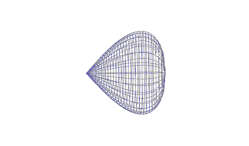
Figure 1. A solid of revolution.

4.2. Ellipsoidal vehicle.

We assume here that the vehicle fills the ellipsoid

$$\mathcal{S}=\Big{\{}y\in\mathbb{R}^{3};\ \ (y_{1}/c_{1})^{2}+(y_{2}/c_{2})^{2}+(y_{3}/c_{3})^{2}\leq 1\}$$ (4.1)

where $c_{1}>c_{2}>c_{3}>0$ denote some numbers. Our first aim is to compute explicitly the functions $\phi_{i}$ and $\varphi_{i}$ for $i=1,2,3$, which solve (2.20)-(2.22) for

$$\Omega=\Big{\{}y\in\mathbb{R}^{3};\ \ (y_{1}/c_{1})^{2}+(y_{2}/c_{2})^{2}+(y_{3}/c_{3})^{2}>1\}.$$

4.2.1. Computations of the functions $\phi_{i}$ and $\varphi_{i}$.

We follow closely [16, pp.148-155]. We introduce a special system of orthogonal curvilinear coordinates, denoted by $(\lambda,\mu,\nu)$, which are defined as the roots of the equation

$$\frac{y_{1}^{2}}{c_{1}^{2}+\theta}+\frac{y_{2}^{2}}{c_{2}^{2}+\theta}+\frac{y_{3}^{2}}{c_{3}^{2}+\theta}-1=0$$ (4.2)

viewed as a cubic in $\theta$. It is clear that (4.2) has three real roots: $\lambda\in(-c_{3}^{2},+\infty)$, $\mu\in(-c_{2}^{2},-c_{3}^{2})$, and $\nu\in(-c_{1}^{2},-c_{2}^{2})$.

It follows immediately from the above definition of $\lambda,\mu,\nu$, that

$$\frac{y_{1}^{2}}{c_{1}^{2}+\theta}+\frac{y_{2}^{2}}{c_{2}^{2}+\theta}+\frac{y_{3}^{2}}{c_{3}^{2}+\theta}-1=\frac{(\lambda-\theta)(\mu-\theta)(\nu-\theta)}{(c_{1}^{2}+\theta)(c_{2}^{2}+\theta)(c_{3}^{2}+\theta)}.$$

This yields

$$\begin{array}[]{ccccc}y_{1}^{2}&=&\displaystyle\frac{(c_{1}^{2}+\lambda)(c_{1}^{2}+\mu)(c_{1}^{2}+\nu)}{(c_{2}^{2}-c_{1}^{2})(c_{3}^{2}-c_{1}^{2})},&&\displaystyle\partial_{\lambda}y_{1}=\displaystyle\frac{1}{2}\frac{y_{1}}{(c_{1}^{2}+\lambda)},\\ \\ y_{2}^{2}&=&\displaystyle\frac{(c_{2}^{2}+\lambda)(c_{2}^{2}+\mu)(c_{2}^{2}+\nu)}{(c_{1}^{2}-c_{2}^{2})(c_{3}^{2}-c_{2}^{2})},&&\displaystyle\partial_{\lambda}y_{2}=\displaystyle\frac{1}{2}\frac{y_{2}}{(c_{2}^{2}+\lambda)},\\ \\ y_{3}^{2}&=&\displaystyle\frac{(c_{3}^{2}+\lambda)(c_{3}^{2}+\mu)(c_{3}^{2}+\nu)}{(c_{1}^{2}-c_{3}^{2})(c_{2}^{2}-c_{3}^{2})},&&\displaystyle\partial_{\lambda}y_{3}=\displaystyle\frac{1}{2}\frac{y_{3}}{(c_{3}^{2}+\lambda)}.\end{array}$$ (4.3)

We introduce the scale factors

$$\begin{array}[]{ccc}h_{\lambda}&=&\displaystyle\frac{1}{2}\sqrt{\frac{(\lambda-\mu)(\lambda-\nu)}{(\lambda+c_{1}^{2})(\lambda+c_{2}^{2})(\lambda+c_{3}^{2})}},\\ \\ h_{\mu}&=&\displaystyle\frac{1}{2}\sqrt{\frac{(\mu-\nu)(\mu-\lambda)}{(\mu+c_{1}^{2})(\mu+c_{2}^{2})(\mu+c_{3}^{2})}},\\ \\ h_{\nu}&=&\displaystyle\frac{1}{2}\sqrt{\frac{(\nu-\lambda)(\nu-\mu)}{(\nu+c_{1}^{2})(\nu+c_{2}^{2})(\nu+c_{3}^{2})}},\\ \\ \end{array}$$ (4.4)

and the function

$$f(\lambda)=\sqrt{(\lambda+c_{1}^{2})(\lambda+c_{2}^{2})(\lambda+c_{3}^{2})}.$$

If $\xi$ is any smooth function of $\lambda$, then its Laplacian is given by

$$\Delta\xi=\frac{4}{(\lambda-\mu)(\lambda-\nu)}f(\lambda)\partial_{\lambda}(f(\lambda)\partial_{\lambda}\xi).$$ (4.5)

according to [16, (7) p. 150]. We search $\phi_{i}$ in the form $\phi_{i}(y_{1},y_{2},y_{3})=y_{i}\xi_{i}(y_{1},y_{2},y_{3})$. Then

$$0=\Delta\phi_{i}=y_{i}\Delta\xi_{i}+2\partial_{i}\xi_{i}.$$ (4.6)

Assuming furthermore that $\xi_{i}$ depends only on $\lambda$, we obtain that

$$\frac{2\partial_{i}\xi_{i}}{y_{i}}=\frac{2\partial_{\lambda}y_{i}}{y_{i}}\frac{\partial_{\lambda}\xi_{i}}{h_{\lambda}^{2}}=\frac{1}{c_{i}^{2}+\lambda}\frac{\partial_{\lambda}\xi_{i}}{h_{\lambda}^{2}}=\frac{4f^{2}(\lambda)}{c_{i}^{2}+\lambda}\frac{\partial_{\lambda}\xi_{i}}{(\lambda-\mu)(\lambda-\nu)}.$$ (4.7)

Combining (4.6) with (4.5) and (4.7), we arrive to

$$0=\partial_{\lambda}(f(\lambda)\partial_{\lambda}\xi_{i})+\frac{1}{c_{i}^{2}+\lambda}f(\lambda)\partial_{\lambda}\xi_{i},$$

which is readily integrated as

$$\xi_{i}=-\hat{C}_{i}\int\limits_{\lambda}^{+\infty}\frac{ds}{(c_{i}^{2}+s)f(s)}+\hat{C}.$$

We choose the constant $\hat{C}=0$ for (2.22) to be fulfilled. As $\partial\Omega$ is represented by the equation $\lambda=0$, then (2.21) reads

$$\partial_{\nu}\phi_{i}=\nu_{i}\Leftrightarrow\xi_{i}\frac{\partial_{\lambda}y_{i}}{y_{i}}+\partial_{\lambda}\xi_{i}=\frac{\partial_{\lambda}y_{i}}{y_{i}}.$$

We infer that $\hat{C}_{i}=c_{1}c_{2}c_{3}/(2-\alpha_{i}),$ where

$$\alpha_{i}=c_{1}c_{2}c_{3}\int\limits_{0}^{+\infty}\frac{ds}{(c_{i}^{2}+s)f(s)}.$$

It is easy seen that

$$\frac{2c_{2}c_{3}}{3c_{1}^{2}}\leq\alpha_{i}\leq\frac{2c_{1}c_{2}}{3c_{3}^{2}}.$$

It follows that if $c_{1},c_{2},c_{3}$ are sufficiently close, then $\alpha_{i}$ is different from $2$, so that $\hat{C}_{i}$ is well defined. We conclude that

$$\phi_{i}(y)=-\frac{\alpha_{i}}{2-\alpha_{i}}y_{i},\;\;\forall y\in\partial\Omega.$$ (4.8)

Let us now proceed to the computation of $\varphi_{i}$. We search $\varphi_{i}$ in the form $\varphi_{i}(y)=\frac{y_{1}y_{2}y_{3}}{y_{i}}\xi_{i}(y)$, where $\xi_{i}$ depends only on $\lambda$. We obtain

$$\Delta\xi_{i}+2\sum_{j=1,j\neq i}^{3}\frac{\partial_{y_{j}}\xi_{i}}{y_{j}}=0\Leftrightarrow\partial_{\lambda}(f(\lambda)\partial_{\lambda}\xi_{i})+\Big{(}\sum_{j=1,j\neq i}^{3}\frac{1}{(c^{2}_{j}+\lambda)}\Big{)}f(\lambda)\partial_{\lambda}\xi_{i}=0,$$

and hence

$$\xi_{i}=-\tilde{C}_{i}\int\limits_{\lambda}^{+\infty}\frac{c_{i}^{2}+s}{f^{3}(s)}ds.$$

From (2.21)-(2.22), we infer that

$$\begin{array}[]{ccc}\displaystyle\tilde{C}_{1}=\frac{c_{1}c_{2}c_{3}(c_{2}^{2}-c_{3}^{2})}{2-\beta_{1}},&&\displaystyle\beta_{1}=c_{1}c_{2}c_{3}(c_{2}^{2}+c_{3}^{2})\int\limits^{+\infty}_{0}\frac{ds}{(c_{2}^{2}+s)(c_{3}^{2}+s)f(s)},\\ \\ \displaystyle\tilde{C}_{2}=\frac{c_{1}c_{2}c_{3}(c_{3}^{2}-c_{1}^{2})}{2-\beta_{2}},&&\displaystyle\beta_{2}=c_{1}c_{2}c_{3}(c_{3}^{2}+c_{1}^{2})\int\limits^{+\infty}_{0}\frac{ds}{(c_{3}^{2}+s)(c_{1}^{2}+s)f(s)},\\ \\ \displaystyle\tilde{C}_{3}=\frac{c_{1}c_{2}c_{3}(c_{1}^{2}-c_{2}^{2})}{2-\beta_{3}},&&\displaystyle\beta_{3}=c_{1}c_{2}c_{3}(c_{1}^{2}+c_{2}^{2})\int\limits^{+\infty}_{0}\frac{ds}{(c_{1}^{2}+s)(c_{2}^{2}+s)f(s)}.\end{array}$$

Note that at the limit case $c_{1}=c_{2}=c_{3}$, we obtain $\beta_{1}=\beta_{2}=\beta_{3}=4/5$. Therefore, if $c_{1},c_{2}$ and $c_{3}$ are near but different, then $\beta_{i}$ is different from $2$, and therefore $\tilde{C}_{i}$ is well defined. We conclude that

$$\varphi_{i}=-\left(\tilde{C}_{i}\int\limits_{0}^{+\infty}\frac{c_{i}^{2}+s}{f^{3}(s)}ds\right)\frac{y_{1}y_{2}y_{3}}{y_{i}},\;\forall y\in\partial\Omega.$$ (4.9)

4.2.2. Controllability of the ellipsoid with six controls

Assume still that $\mathcal{S}$ is given by (4.1). Note that $\mathcal{S}$ is symmetric with respect to the plane $\{y_{p}=0\}$ for $p=1,2,3$. Assume given six functions $\chi_{j}$, $j=1,\ldots,6$, each being symmetric with respect to the plane $\{y_{p}=0\}$ for $p=1,2,3$, with

$$\varepsilon_{\chi_{1}}^{p}=\left\{\begin{array}[]{cc}-1&p=1\\ 1&p=2\\ 1&p=3\end{array}\right., \varepsilon_{\chi_{2}}^{p}=\left\{\begin{array}[]{cc}1&p=1\\ -1&p=2\\ 1&p=3\end{array}\right., \varepsilon_{\chi_{3}}^{p}=\left\{\begin{array}[]{cc}1&p=1\\ 1&p=2\\ -1&p=3\end{array}\right.,$$ (4.19)

$$\varepsilon_{\chi_{4}}^{p}=\left\{\begin{array}[]{cc}1&p=1\\ -1&p=2\\ -1&p=3\end{array}\right., \varepsilon_{\chi_{5}}^{p}=\left\{\begin{array}[]{cc}-1&p=1\\ 1&p=2\\ -1&p=3\end{array}\right., \varepsilon_{\chi_{6}}^{p}=\left\{\begin{array}[]{cc}-1&p=1\\ -1&p=2\\ 1&p=3\end{array}\right..$$ (4.29)

To obtain this kind of controls in practice, we can proceed as follows:

• We build six tunnels in the rigid body, as drawn in Figure 2.

  

  Figure 2. Ellipsoid with six controls.

• We divide the six tunnels in three groups of two parallel tunnels; that is, we put together the tunnels located in the same plane (see Figure 3).

  

  

  

  

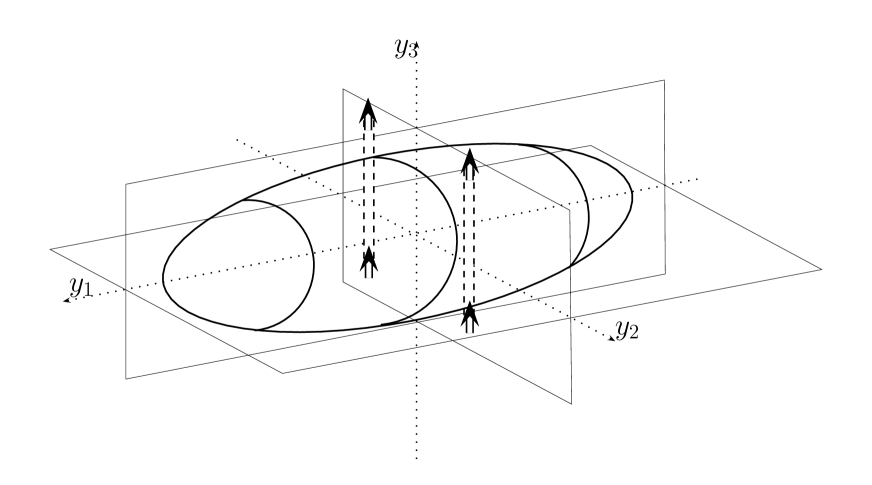
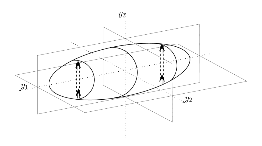
  Figure 3. Independent controls in each plane.

• Let $\tilde{w}_{1}$ and $\tilde{w}_{2}$ denote the effective flow controls in the two tunnels located in the plane $\{y_{3}=0\}$. They may appear together in (1.21) as $\tilde{w}_{1}\chi(y_{1},y_{2},y_{3})+\tilde{w}_{2}\chi(y_{1},-y_{2},y_{3})$, where $\chi\in C^{\infty}(\partial\Omega)$ is some function with

  $$\textrm{Supp }\chi\subset\{y_{2}>0\},\quad\varepsilon_{\chi}^{1}=-1,\quad\textrm{and}\quad\varepsilon_{\chi}^{3}=1.$$

  We introduce the (new) support functions

  $$\chi_{1}(y_{1},y_{2},y_{3}) = \chi(y_{1},y_{2},y_{3})+\chi(y_{1},-y_{2},y_{3}),$$

  $$\chi_{6}(y_{1},y_{2},y_{3}) = \chi(y_{1},y_{2},y_{3})-\chi(y_{1},-y_{2},y_{3})$$

  and the (new) control inputs

  $$w_{1} = \frac{\tilde{w}_{1}+\tilde{w}_{2}}{2},$$

  $$w_{6} = \frac{\tilde{w}_{1}-\tilde{w}_{2}}{2}.$$

  (See Figure 4.) Then (4.29) is satisfied for $\chi_{1}$ and $\chi_{6}$, and

  $$\tilde{w}_{1}\chi(y_{1},y_{2},y_{3})+\tilde{w}_{2}\chi(y_{1},-y_{2},y_{3})=w_{1}\chi_{1}(y_{1},y_{2},y_{3})+w_{6}\chi_{6}(y_{1},y_{2},y_{3}).$$

  The same can be done in the other planes $\{y_{1}=0\}$ and $\{y_{2}=0\}$.

  

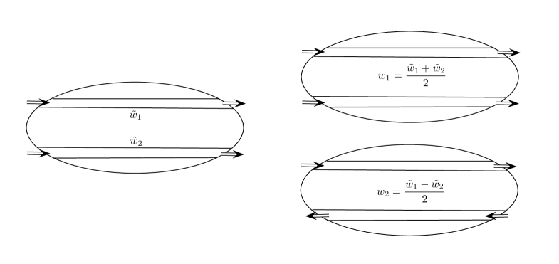
  Figure 4. Definition of the new controls in the plane $\{y_{3}=0\}$.

We notice that $C$ is a diagonal matrix:

$$C=-\textrm{diag}(C_{1},C_{2},C_{3},C_{4},C_{5},C_{6}),$$

with

$$C_{i}=\int\limits_{\partial\Omega}\phi_{i}\chi_{i},\;i=1,2,3,\quad\text{and}\quad C_{i+3}=\int\limits_{\partial\Omega}\varphi_{i}\chi_{i+3},\;i=1,2,3.$$

From (4.8)-(4.9), there are some constants $\bar{C}_{i}\neq 0$, $i=1,...,6$, which depend only on $c_{1},c_{2}$ and $c_{3}$, such that

$$C_{i}=\bar{C}_{i}\int\limits_{\partial\Omega\cap(0,+\infty)^{3}}{y_{i}\chi_{i}}(y),\;\;\;\;C_{i+3}=\bar{C}_{i+3}\int\limits_{\partial\Omega\cap(0,+\infty)^{3}}\left(\frac{y_{1}y_{2}y_{3}}{y_{i}}\right)\chi_{i+3}(y),\;\;\;i=1,2,3.$$ (4.30)

By (4.30), we have that $C_{i}\neq 0$ for $i=1,...,6$, and hence rank$(C)=6$ if, in addition to (4.29), it holds

$$\chi_{i}\not\equiv 0,\ i=1,...,6,$$ (4.31)

$$\chi_{i}\geq 0\text{ on }\partial\Omega\cap(0,+\infty)^{3},\ i=1,...,6.$$ (4.32)

By Proposition 3.1 and Theorem 3.11, it follows that both the linearized system (3.1) and the nonlinear system (2.68) are (locally) controllable.

Remark 4.1.

Since $\varepsilon_{\chi_{1}}^{1}=(-1)^{\delta_{11}}=-1$, we have that $(L_{1}^{M})_{11}=(W_{1}^{M})_{11}=0$, and hence $\beta=\gamma=0$. Thus $\gamma+\alpha\beta=0$. Proceeding as in [12, Theorem 2.2], one can prove that, under certain rank conditions, two arbitrary states of the form $(h,\vec{q},0,0)$ can be connected by trajectories of the ellipsoid in (sufficiently) large time.

In the following sections, we shall be concerned with the controllability of the ellipsoid with less controls (namely, $4$ controls and $3$ controls). If, in the pair $(\chi_{1},\chi_{6})$, only $\chi_{6}$ is available, then $\chi_{6}$ can be generated as above by two propellers controlled in the same way (Figure 5 left), or by only one propeller by choosing an appropriate scheme for the tunnels (Figure 5 middle). In what follows, to indicate that the flows in the two tunnels are linked, we draw a transversal line in bold between the two tunnels (Figure 5 right).

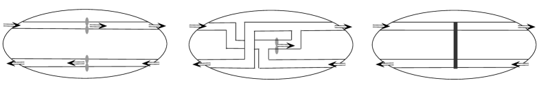
Figure 5. Two ways to generate $\chi_{6}$.

4.2.3. Controllability of the ellipsoid with four controls

We consider the same controllers $\chi_{1},\chi_{4},\chi_{5}$ and $\chi_{6}$ as above, still satisfying (4.29), (4.31), (4.32). (See Figure 6.)

Control $\chi_{1}$

Control $\chi_{4}$

Control $\chi_{5}$

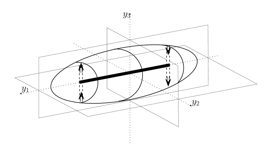
Control $\chi_{6}$

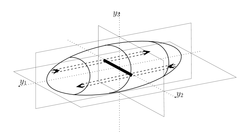
Figure 6. Ellipsoid with four controls.

If the density $\rho$ is scaled by a factor $\lambda$, i.e. $\rho(x)$ is replaced by $\rho^{\lambda}(x)=\lambda\rho(x)$ where $\lambda>0$, then the mass and the inertia matrix are scaled in the same way; that is, $m_{0}$ and $J_{0}$ are replaced by

$$m_{0}^{\lambda}=\lambda m_{0},\quad J_{0}^{\lambda}=\lambda J_{0}.$$

Thus, if $\lambda\to\infty$, then $m_{0}^{\lambda}\to\infty$, $[J_{0}^{\lambda}]^{-1}\to 0$, and $[{\mathcal{J}}^{\lambda}]^{-1}\to 0$. (Note that large values of $\lambda$ are not compatible with the neutral buoyancy, but they prove to be useful to identify geometric configurations leading to controllability results with less than six control inputs.)

Note that the matrices $M,J,N,C^{M},C^{J},L_{p}^{M},R_{p}^{M},W_{p}^{M},L_{p}^{J},R_{p}^{J},W_{p}^{J}$ keep constant when $\lambda\to\infty$. In particular,

$$\lim_{\lambda\to\infty}{\bf A}{\mathcal{J}}^{-1}C=0,\quad\lim\frac{1}{2}{\mathcal{J}}{\bf D}{\mathcal{J}}^{-1}C=0.$$

Let $B^{\infty}=\lim\limits_{\lambda\to\infty}{\bf B}$. Then $B^{\infty}$ and $C$ are given by

$$\begin{array}[]{cc}B^{\infty}=-\left(\begin{array}[]{cccc}0&0&0&0\\ 0&0&0&B_{6}\\ 0&0&B_{5}&0\\ 0&0&0&0\\ 0&0&0&0\\ 0&0&0&0\end{array}\right),&C=-\left(\begin{array}[]{cccc}C_{1}&0&0&0\\ 0&0&0&0\\ 0&0&0&0\\ 0&C_{4}&0&0\\ 0&0&C_{5}&0\\ 0&0&0&C_{6}\end{array}\right),\end{array}$$

with

$$B_{5}=\int\limits_{\partial\Omega}\left(\nabla\psi_{1}\cdot\nabla\psi_{5}\right)\nu_{3},\;\;\;B_{6}=\int\limits_{\partial\Omega}\left(\nabla\psi_{1}\cdot\nabla\psi_{6}\right)\nu_{2}.$$

Thus, if $B_{5}\neq 0$ and $B_{6}\neq 0$, we see that (3.81) and (3.82) are fulfilled, so that the local controllability of (2.68) is ensured by Corollary 3.12 for $\lambda$ large enough. We note then that the matrix in $\mathbb{R}^{6\times 6}$ obtained by gathering together the four columns of $C$ and the last two columns of $B^{\infty}$ is invertible. Let $R_{1}(\lambda)\in\mathbb{R}^{6\times 6}$ (resp. $R_{2}(\lambda)\in\mathbb{R}^{6\times 6}$) denote the matrix obtained by gathering together the four columns of $C$ with the last two columns of ${\bf B}+{\bf A}{\mathcal{J}}^{-1}C$ (resp. with the last two columns of $\frac{1}{2}{\mathcal{J}}{\bf D}{\mathcal{J}}^{-1}C+{\bf B}+{\bf A}{\mathcal{J}}^{-1}C$). Then for $\lambda\gg 1$, we have

$$\textrm{det }R_{1}(\lambda)\neq 0\quad\textrm{ and }\quad\textrm{det }R_{2}(\lambda)\neq 0.$$

Since the coefficients of $R_{1}(\lambda),R_{2}(\lambda)$ are rational functions of $\lambda$, we infer that the equation

$$\textrm{det }R_{1}(\lambda)\cdot\textrm{det }R_{2}(\lambda)=0$$

is an algebraic equation in $\lambda$. Therefore, it has at most a finite set of roots in $(0,+\infty)$, that we denote by $\Lambda_{critical}$. We conclude that for any $\lambda\in(0,+\infty)\setminus\Lambda_{critical}$, the local controllability of (2.68) still holds. In particular, we can consider values of $\lambda$ arbitrary close to the value $\lambda=1$ imposed by (1.10). The issue whether $1\in\Lambda_{critical}$ seems hard to address without computing numerically all the coefficients in our system.

4.2.4. Controllability of the ellipsoid with three controls

Assume that $\chi_{1},\chi_{4},\chi_{5}$ and $\chi_{6}$ are as above (satisfying (4.29), (4.31), (4.32)), and consider now the controls supported by $\chi_{1}$, $\chi_{4}$ and $\tilde{\chi}_{5}=\chi_{5}+\chi_{6}$ (see Figure 7).

Control $\chi_{1}$

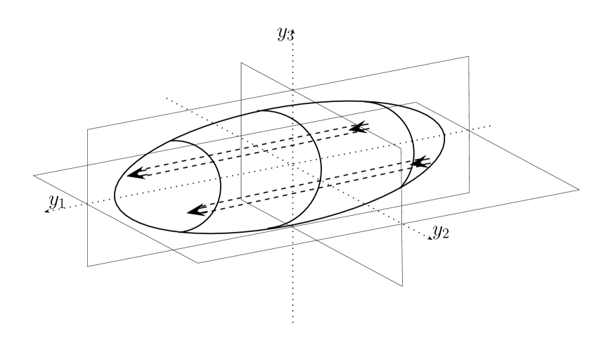
Control $\chi_{4}$

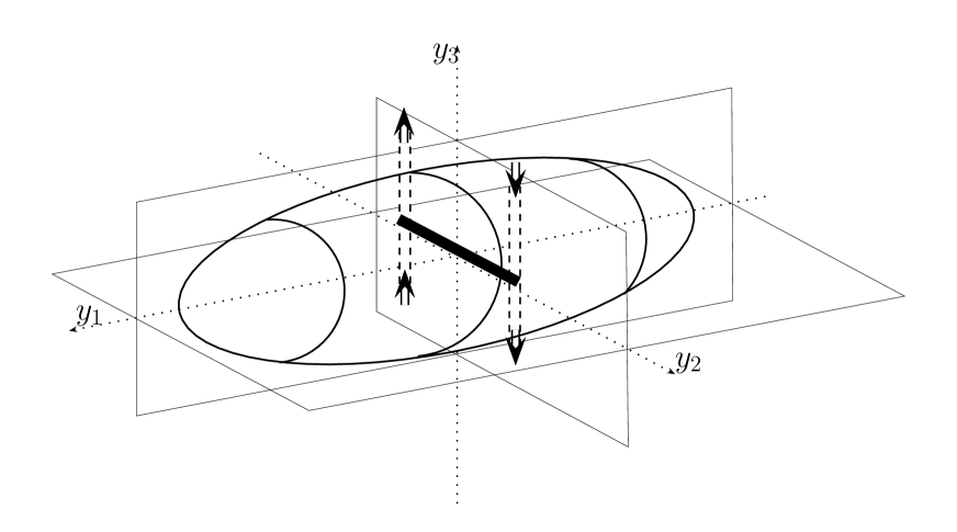
Control $\tilde{\chi}_{5}$

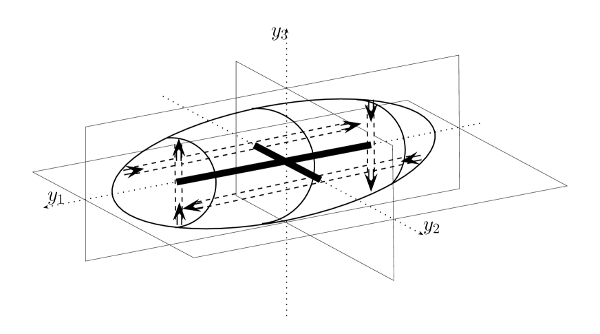
Figure 7. Ellipsoid with three controls.

Doing the same scaling for the density, and letting $\lambda\to\infty$, we see that the matrices $B^{\infty}$ and $C$ read

$$\begin{array}[]{cc}B^{\infty}=-\left(\begin{array}[]{cccc}0&0&0\\ 0&0&B_{6}\\ 0&0&B_{5}\\ 0&0&0\\ 0&0&0\\ 0&0&0\end{array}\right),&C=-\left(\begin{array}[]{ccc}C_{1}&0&0\\ 0&0&0\\ 0&0&0\\ 0&C_{4}&0\\ 0&0&C_{5}\\ 0&0&C_{6}\end{array}\right),\end{array}$$

where the coefficients $B_{5},B_{6},C_{1},C_{4},C_{5},C_{6}$ are as above. For simplicity, we assume that the principal axes of inertia of the vehicule coincide with the axes of the ellipsoid. Then the matrix $J_{0}$ is diagonal (see [4]) with entries $J_{1},J_{2},J_{3}$. Notice that the first and fourth coordinates are well controlled (using $\chi_{1}$ and $\chi_{4}$), and that the other coordinates are decoupled from them, at least asymptotically (i.e. when $\lambda\to\infty$). Let $A^{\infty}=\lim_{\lambda\to\infty}{\bf A}$ (i.e. $A^{\infty}$ is obtained by letting $\alpha=0$ in ${\bf A}$). Let $K\in\mathbb{R}^{4\times 4}$ denote the matrix obtained from $A^{\infty}$ by removing the first and fourth lines (resp. columns), and let $b\in\mathbb{R}^{4}$ (resp. $c\in\mathbb{R}^{4}$) denote the vector obtained from the last column of $B^{\infty}$ (resp. $C$) by removing the first and fourth coordinates, namely

$$K=\left(\begin{array}[]{cccc}-(L_{1}^{M})_{22}&0&0&-(R_{1}^{M})_{23}\\ 0&-(L_{1}^{M})_{33}&-(R_{1}^{M})_{32}&0\\ 0&-((L_{1}^{J})_{23}+(C^{M})_{11})&-(R_{1}^{J})_{22}&0\\ -((L_{1}^{J})_{32}-(C^{M})_{11})&0&0&-(R_{1}^{J})_{33}\end{array}\right),$$

$$b=\left(\begin{array}[]{cccc}B_{6}\\ B_{5}\\ 0\\ 0\end{array}\right),\qquad c=\left(\begin{array}[]{cccc}0\\ 0\\ C_{5}\\ C_{6}\end{array}\right).$$

Let finally

$$F=\left(\begin{array}[]{cccc}0&0&0&-1\\ 0&0&1&0\\ 0&0&0&0\\ 0&0&0&0\end{array}\right)\quad\text{ and }G=\left(\begin{array}[]{cccc}m_{0}^{-1}&0&0&0\\ 0&m_{0}^{-1}&0&0\\ 0&0&J_{2}^{-1}&0\\ 0&0&0&J_{3}^{-1}\end{array}\right).$$

Then, keeping only the leading terms as $\lambda\to\infty$, we see that (3.85) holds if

$$\textrm{rank }(c,b,KGb,(KG)^{2}b,(KG)^{3}b)=4$$ (4.35)

while (3.86) holds if

$$\textrm{rank }\bigg{(}c,b,[(C^{M})_{11}F+2K]Gb,[8(C^{M})_{11}F+11K]GKGb,\\ [17(C^{M})_{11}F+64K]G(KG)^{2}b\bigg{)}=4.$$ (4.36)

Note that (4.35) is satisfied whenever

$$\textrm{rank}(b,KGb,(KG)^{2}b,(KG)^{3}b)=4,$$ (4.37)

which is nothing but the Kalman rank condition for the system $\dot{x}=KGx+bu$. However, it is clear that we should take advantage of the presence $c$ in (4.35). As previously, this gives a controllability result for $\lambda\gg 1$, but such a result is also valid for all the positive $\lambda$’s except those in a finite set defined by an algebraic equation.

5. Appendix

5.1. Quaternions and rotations.

Quaternions are a convenient tool for representing rotations of objects in three dimensions. For that reason, they are widely used in robotic, navigation, flight dynamics, etc. (See e.g. [1, 24]). We limit ourselves to introducing the few definitions and properties needed to deal with the dynamics of $h$ and $Q$. (We refer the reader to [1] for more details.)

The set of quaternions, denoted by $\mathbb{H}$, is a noncommutative field containing $\mathbb{C}$ and which is a $\mathbb{R}$-algebra of dimension 4. Any quaternion $q\in\mathbb{H}$ may be written as

$$q=q_{0}+q_{1}i+q_{2}j+q_{3}k,$$

where $(q_{0},q_{1},q_{2},q_{3})\in\mathbb{R}^{4}$ and $i,j,k\in\mathbb{H}$ are some quaternions whose products will be given later. We say that $q_{0}$ (resp. $q_{1}i+q_{2}j+q_{3}k$) is the real part (resp. the imaginary part) of $q$. Identifying the imaginary part $q_{1}i+q_{2}j+q_{3}k$ with the vector $\vec{q}=(q_{1},q_{2},q_{3})\in\mathbb{R}^{3}$, we can represent the quaternion $q$ as $q=[q_{0},\vec{q}\,]$, where $q_{0}\in\mathbb{R}$ (resp. $\vec{q}\in\mathbb{R}^{3}$) is the scalar part (resp. the vector part) of $q$. The addition, scalar multiplication and quaternion multiplication are defined respectively by

$$[p_{0},\vec{p}\,]+[q_{0},\vec{q}\,]=[p_{0}+q_{0},\vec{p}+\vec{q}\,],$$

$$t[q_{0},\vec{q}\,]=[tq_{0},t\vec{q}\,],$$

$$[p_{0},\vec{p}\,]*[q_{0},\vec{q}\,]=[p_{0}q_{0}-\vec{p}\cdot\vec{q},p_{0}\vec{q}+q_{0}\vec{p}+\vec{p}\times\vec{q}\,],$$

where “$\cdot$” is the dot product and “$\times$” is the cross product. We stress that the quaternion multiplication $*$ is not commutative. Actually, we have that

$$i*j=k,\quad j*i=-k,$$

$$j*k=i,\quad k*j=-i,$$

$$k*i=j,\quad i*k=-j,$$

$$i^{2}=j^{2}=k^{2}=-1.$$

Any pure scalar $q_{0}$ and any pure vector $\vec{q}$ may be viewed as quaternions

$$q_{0}=[q_{0},\vec{0}\,],\qquad\vec{q}=[0,\vec{q}\,],$$

and hence any quaternion $q=[q_{0},\vec{q}\,]$ can be written as the sum of a scalar and a vector, namely

$$q=q_{0}+\vec{q}.$$

The cross product of vectors extends to quaternions by setting

$$p\times q=\frac{1}{2}(p*q-q*p)=[0,\vec{p}\times\vec{q}\,].$$

The conjugate of a quaternion $q=[q_{0},\vec{q}\,]$ is $q^{*}=[q_{0},-\vec{q}\,]$. The norm of $q$ is

$$||q||=(|q_{0}|^{2}+||\vec{q}\,||^{2})^{\frac{1}{2}}.$$

From

$$q*q^{*}=q^{*}*q=||q||^{2},$$

we infer that

$$q^{-1}=\frac{q^{*}}{||q||^{2}}\cdot$$

A unit quaternion is a quaternion of norm 1. The set of unit quaternions may be identified with $S^{3}$. It is a group for $*$.

Any unit quaternion $q=[q_{0},\vec{q}\,]$ can be written in the form

$$q=\cos\frac{\alpha}{2}+\sin\frac{\alpha}{2}\vec{u},$$ (5.1)

where $\alpha\in\mathbb{R}$ and $\vec{u}\in\mathbb{R}^{3}$ with $||\vec{u}||=1$. Note that the writing is not unique: if the pair $(\alpha,\vec{u}\,)$ is convenient, the same is true for the pairs $(-\alpha,-\vec{u}\,)$ and $(\alpha+4k\pi,\vec{u}\,)$ $(k\in\mathbb{Z})$, as well. However, if we impose that $\alpha\in[0,2\pi]$, then $\alpha$ is unique, and $\vec{u}$ is unique for $|q_{0}|<1$. (However, any $\vec{u}\in S^{3}$ is convenient for $|q_{0}|=1$.)

For any unit quaternion $q$, let the matrix $R(q)\in\mathbb{R}^{3\times 3}$ be defined by

$$R(q){\vec{v}}=q*{\vec{v}}*q^{*}\quad\forall{\vec{v}}\in\mathbb{R}^{3}.$$ (5.2)

Then $R(q)$ is found to be

$$R(q)=\left(\begin{array}[]{ccc}q_{0}^{2}+q_{1}^{2}-q_{2}^{2}-q_{3}^{2}&2(q_{1}q_{2}-q_{0}q_{3})&2(q_{1}q_{3}+q_{0}q_{2})\\ 2(q_{2}q_{1}+q_{0}q_{3})&q_{0}^{2}-q_{1}^{2}+q_{2}^{2}-q_{3}^{2}&2(q_{2}q_{3}-q_{0}q_{1})\\ 2(q_{3}q_{1}-q_{0}q_{2})&2(q_{3}q_{2}+q_{0}q_{1})&q_{0}^{2}-q_{1}^{2}-q_{2}^{2}+q_{3}^{2}\end{array}\right).$$

For $q$ given by (5.1), then $R(q)$ is the rotation around the axis $\mathbb{R}\vec{u}$ of angle $\alpha$.

Note that $R(q_{1}*q_{2})=R(q_{1})R(q_{2})$ (i.e. $R$ is a group homomorphism), hence

$$R(1)=Id,\quad R(q^{*})=R(q)^{-1}.$$

We notice that the map $q\to R(q)$ from the unit quaternions set $S^{3}$ to $SO(3)$ is onto, but not one-to-one, for $R(-q)=R(q)$. It becomes one-to-one when restricted to the open set

$$S^{3}_{+}:=\{q=[q_{0},\vec{q}\,]\in{\mathbb{H}};\ ||q||=1\text{ and }q_{0}>0\}.$$

Furthermore, the map $R$ is a smooth invertible map from $S^{3}_{+}$ onto an open neighbourhood $\mathcal{O}$ of $Id$ in $SO(3)$. On the other hand, the map

$$\vec{q}\to q=[q_{0},\vec{q}\,]=[\sqrt{1-||\vec{q}\,||^{2}},\vec{q}\,]$$

is a smooth invertible map from the unit ball $B_{1}(0)=\{\vec{q}\in\mathbb{R}^{3};\ ||\vec{q}\,||<1\}$ onto $S^{3}_{+}$. Thus the rotations in $\mathcal{O}$ can be parameterized by $\vec{q}\in B_{1}(0)$.

5.2. Proof of Proposition 3.10.

Let us prove by induction on $k\in\mathbb{N}$ that

$$V_{2k}^{(2l)}(T)=0\qquad\forall l\in\mathbb{N}.$$ (5.3)

The property is clearly true for $k=0$, since

$$V_{0}^{(2l)}(T)=\hat{B}^{(2l)}(T)+\hat{A}^{(2l)}(T)\hat{C}=0,$$

by (3.70). Assume that (5.3) is established for some $k\in\mathbb{N}$. Then by (3.69) applied twice, we have

$$V_{2k+2}=V_{2k}^{\prime\prime}-2\hat{A}V_{2k}^{\prime}-\hat{A}^{\prime}V_{2k}+\hat{A}^{2}V_{2k},$$

hence

$$V_{2k+2}^{(2l)}(T)=V_{2k}^{(2l+2)}-2(\hat{A}V_{2k}^{\prime})^{(2l)}(T)-(\hat{A}^{\prime}V_{2k})^{(2l)}(T)+(\hat{A}^{2}V_{2k})^{(2l)}(T).$$ (5.4)

The first term in the r.h.s. of (5.4) is null by (5.3). The second one is also null, for by Leibniz’ rule

$$(\hat{A}V^{\prime}_{2k})^{(2l)}(T)=\sum_{p=0}^{2l}C_{2l}^{p}\hat{A}^{(p)}(T)V_{2k}^{(2l-p+1)}(T)$$

and $\hat{A}^{(p)}(T)=0$ if $p$ is even, while $V_{2k}^{(2l-p+1)}(T)=0$ if $p$ is odd. One proves in a similar way that the third and fourth terms in the r.h.s. of (5.4) are null, noticing that for $p$ odd we have

$$(\hat{A}^{2})^{(p)}(T)=2(\hat{A}\hat{A}^{\prime})^{(p-1)}(T)=0.$$ (5.5)

From (5.3), we infer that

$$V_{2k+1}^{(2l+1)}(T)=V_{2k}^{(2l+2)}(T)-(\hat{A}V_{2k})^{(2l+1)}(T)=0.$$

Let us proceed to the proof of (3.72). Again, we first prove by induction on $k\in\mathbb{N}$ that

$$U_{2k+1}^{(2l)}(T)=0\qquad\forall l\in\mathbb{N}.$$ (5.6)

It follows from (3.68), (3.69) and (3.71) that

$$U_{1}^{(2l)}(T)=U_{0}^{(2l+1)}(T)-(DU_{0})^{(2l)}(T)-V_{0}^{(2l)}(T)=0\qquad\forall k\in\mathbb{N}.$$

Assume that (5.6) is true for some $k\in\mathbb{N}$. Then, by (3.69) applied twice,

$$U_{2k+3}^{(2l)}(T)=U_{2k+1}^{(2l+2)}(T)-(DU_{2k+1})^{(2l+1)}(T)-V_{2k+1}^{(2l+1)}(T)-(DU_{2k+2})^{(2l)}(T)-V_{2k+2}^{(2l)}(T).$$ (5.7)

Using (3.70), (3.71) and (5.6), we see that all the terms in the r.h.s. of (5.7), except possibly $(DU_{2k+2})^{(2l)}(T)$, are null. Finally,

$$(DU_{2k+2})^{(2l)}(T)=(DU_{2k+1}^{\prime})^{(2l)}(T)-(D^{2}U_{2k+1})^{(2l)}(T)-(DV_{2k+1})^{(2l)}(T).$$

Using Leibniz’ rule for each term, noticing that in each pair $(p,q)$ with $p+q=2l$, $p$ and $q$ are simultaneously even or odd, and using (3.70), (3.71), (5.5) (with $\hat{A}$ replaced by $D$), and (5.6), we conclude that $(DU_{2k+2})^{(2l)}(T)=0$, so that $U_{2k+3}^{(2l)}(T)=0$.

Finally, $U_{2k}^{(2l+1)}(T)=0$ is obvious for $k=0$, while for $k\geq 1$

$$U_{2k}^{(2l+1)}(T)=U_{2k-1}^{(2l+2)}(T)-(DU_{2k-1})^{(2l+1)}(T)-V_{2k-1}^{(2l+1)}(T)=0$$

by (3.70), (3.71) and (5.6) (with $2k+1$ replaced by $2k-1$). The proof of Proposition 3.10 is complete.

5.3. Proof of Proposition 3.14

From (3.67), (3.68) and (3.83), we obtain successively

$$V_{1}(T) = V_{0}^{\prime}(T)=\hat{B}^{\prime}(T)+\hat{A}^{\prime}(T)\hat{C}=\overline{w_{1}}^{\prime}(T)\big{(}{\mathcal{J}}^{-1}{\bf B}+{\mathcal{J}}^{-1}{\bf A}{\mathcal{J}}^{-1}C\big{)}$$

$$V_{3}(T) = V_{2}^{\prime}(T)$$

$$= (V_{1}^{\prime}-\hat{A}V_{1})^{\prime}(T)$$

$$= (V_{0}^{\prime}-\hat{A}V_{0})^{\prime\prime}(T)-(\hat{A}V_{1})^{\prime}(T)$$

$$= V_{0}^{\prime\prime\prime}(T)-2\hat{A}^{\prime}(T)V_{0}^{\prime}(T)-\hat{A}^{\prime}(T)V_{1}(T)$$

$$= -3\hat{A}^{\prime}(T)V_{0}^{\prime}(T).$$

Successive applications of (3.68) yield

$$V_{5}(T) = V_{0}^{(5)}(T)-\sum_{i=0}^{3}(\hat{A}V_{i})^{(4-i)}(T),$$ (5.8)

$$V_{7}(T) = V_{0}^{(7)}(T)-\sum_{i=0}^{5}(\hat{A}V_{i})^{(6-i)}(T).$$ (5.9)

Since $V_{0}^{(k)}(T)=0$ for $k\geq 2$, it remains to estimate the terms $(\hat{A}V_{i})^{(4-i)}(T)$ and $(\hat{A}V_{i})^{(6-i)}(T)$. Notice first that by (3.83) and Leibniz’ rule

$$(\hat{A}V_{i})^{(k)}(T)=k\hat{A}^{\prime}(T)V_{i}^{(k-1)}(T).$$

Thus, from (3.83) and (3.88), we have that

$$(\hat{A}V_{0})^{(4)}(T)=0,$$ (5.10)

$$(\hat{A}V_{1})^{(3)}(T)=3\hat{A}^{\prime}(T)V_{1}^{\prime\prime}(T)=3\hat{A}^{\prime}(T)\big{(}V_{0}^{(3)}(T)-(\hat{A}V_{0})^{\prime\prime}(T)\big{)}=-6\hat{A}^{\prime}(T)^{2}V_{0}^{\prime}(T),\qquad$$ (5.11)

$$(\hat{A}V_{2})^{\prime\prime}(T)=2\hat{A}^{\prime}(T)V_{2}^{\prime}(T)=2\hat{A}^{\prime}(T)V_{3}(T)=-6\hat{A}^{\prime}(T)^{2}V_{0}^{\prime}(T),$$ (5.12)

$$(\hat{A}V_{3})^{\prime}(T)=\hat{A}^{\prime}(T)V_{3}(T)=-3\hat{A}^{\prime}(T)^{2}V_{0}^{\prime}(T).$$ (5.13)

This yields (3.89). On the other hand,

$$(\hat{A}V_{0})^{(6)}(T) = 0,$$ (5.14)

$$(\hat{A}V_{1})^{(5)}(T) = 5\hat{A}^{\prime}(T)V_{1}^{(4)}(T)=5\hat{A}^{\prime}(T)\big{(}V_{0}^{(5)}-(\hat{A}V_{0})^{(4)}\big{)}(T)=0,$$ (5.15)

$$(\hat{A}V_{2})^{(4)}(T) = 4\hat{A}^{\prime}(T)V_{2}^{(3)}(T).$$ (5.16)

Since

$$V_{2}=V_{1}^{\prime}-\hat{A}V_{1}=V_{0}^{\prime\prime}-(\hat{A}V_{0})^{\prime}-\hat{A}V_{1},$$

we obtain with (3.83) and (5.11) that

$$V_{2}^{(3)}(T)=V_{0}^{(5)}(T)-(\hat{A}V_{0})^{(4)}(T)-(\hat{A}V_{1})^{(3)}(T)=6\hat{A}^{\prime}(T)^{2}V_{0}^{\prime}(T),$$

hence

$$(\hat{A}V_{2})^{(4)}(T)=24\hat{A}^{\prime}(T)^{3}V_{0}^{\prime}(T).$$ (5.17)

On the other hand,

$$(\hat{A}V_{3})^{(3)}(T) = 3\hat{A}^{\prime}(T)V_{3}^{\prime\prime}(T)$$ (5.18)

$$= 3\hat{A}^{\prime}(T)\big{(}V_{4}^{\prime}(T)+(\hat{A}V_{3})^{\prime}(T)\big{)}$$

$$= 3\hat{A}^{\prime}(T)\big{(}V_{5}(T)+\hat{A}^{\prime}(T)V_{3}(T)\big{)}$$

$$= 36\hat{A}^{\prime}(T)^{3}V_{0}^{\prime}(T)$$

where we used (3.68) and (3.88)-(3.89). Finally,

$$(\hat{A}V_{4})^{\prime\prime}(T)=2\hat{A}^{\prime}(T)V_{4}^{\prime}(T)=2\hat{A}^{\prime}(T)V_{5}(T)=30\hat{A}^{\prime}(T)^{3}V_{0}^{\prime}(T)$$ (5.19)

and

$$(\hat{A}V_{5})^{\prime}(T)=\hat{A}^{\prime}(T)V_{5}(T)=15\hat{A}^{\prime}(T)V_{0}^{\prime}(T).$$ (5.20)

Gathering together (5.9) and (5.14)-(5.20), we obtain (3.90). The proof of Proposition 3.14 is complete.

5.4. Proof of Proposition 3.15

From (3.68)-(3.69), we have that

$$U_{0}\equiv\hat{C},\qquad U_{i}=U_{i-1}^{\prime}-DU_{i-1}-V_{i-1},\quad\forall i\geq 1.$$ (5.21)

Thus

$$U_{2}(T) = (U_{1}^{\prime}-DU_{1}-V_{1})(T)$$

$$= (0-(DU_{0})^{\prime}-V_{0}^{\prime})(T)-V_{1}(T)$$

$$= -D^{\prime}(T)U_{0}-2V_{0}^{\prime}(T)$$

where we used successively (5.21), (3.72) and (3.87).

Successive applications of (5.21) yield

$$U_{4}(T)=-\sum_{i=0}^{3}[(DU_{i})^{(3-i)}+V_{i}^{(3-i)}](T).$$ (5.22)

Using (3.83), we obtain that

$$\sum_{i=0}^{3}(DU_{i})^{(3-i)}(T) = \sum_{i=0}^{2}(3-i)D^{\prime}(T)U_{i}^{(2-i)}(T)$$ (5.23)

$$= 2D^{\prime}(T)\big{(}U_{2}(T)+V_{1}(T)\big{)}+D^{\prime}(T)V_{0}^{\prime}(T)$$

$$= -3D^{\prime}(T)\big{(}D^{\prime}(T)U_{0}+2V_{0}^{\prime}(T)\big{)}+2D^{\prime}(T)V_{0}^{\prime}(T)$$

$$= -4D^{\prime}(T)V_{0}^{\prime}(T)$$

where we used (3.87), (3.91) and the fact that $D^{\prime}(T)^{2}=0$.

On the other hand,

$$\sum_{i=0}^{3}V_{i}^{(3-i)}(T) = (V_{0}^{\prime}-\hat{A}V_{0})^{\prime\prime}(T)+V_{2}^{\prime}(T)+V_{3}(T)$$ (5.24)

$$= -2\hat{A}^{\prime}(T)V_{0}^{\prime}(T)+2V_{3}(T)$$

$$= -8\hat{A}^{\prime}(T)V_{0}^{\prime}(T)$$

by (3.88). Combining (5.22)-(5.24), we obtain (3.92).

Let us now compute $U_{6}(T)$. Successive applications of (5.21) yield

$$U_{6}(T)=-\sum_{i=0}^{5}[(DU_{i})^{(5-i)}+V_{i}^{(5-i)}](T).$$ (5.25)

We have that

$$\sum_{i=0}^{5}(DU_{i})^{(5-i)}(T)=\sum_{i=0}^{4}(5-i)D^{\prime}(T)U_{i}^{(4-i)}(T).$$

Let us estimate the terms $U_{i}^{(4-i)}(T)$ for $i=0,...,4$. Obviously, $U_{0}^{(4)}(T)=0$ by (5.21), while by (3.83)

$$U_{1}^{(3)}(T)=-(DU_{0})^{(3)}(T)-V_{0}^{(3)}(T)=0.$$ (5.26)

Next we use (5.21) to obtain successively

$$U_{3}^{\prime}(T) = U_{4}(T)+V_{3}(T),$$ (5.27)

$$U_{2}^{\prime\prime}(T) = U_{3}^{\prime}(T)+(DU_{2})^{\prime}(T)+V_{2}^{\prime}(T)$$

$$= U_{4}(T)+V_{3}(T)+D^{\prime}(T)U_{2}(T)+V_{3}(T).$$

It follows that

$$\sum_{i=0}^{4}(DU_{i})^{(5-i)}(T)$$

$$\qquad=3D^{\prime}(T)\big{(}U_{4}(T)+2V_{3}(T)+D^{\prime}(T)U_{2}(T)\big{)}+2D^{\prime}(T)\big{(}U_{4}(T)+V_{3}(T)\big{)}+D^{\prime}(T)U_{4}(T)$$

$$\qquad=D^{\prime}(T)\big{(}6U_{4}(T)+8V_{3}(T)\big{)}$$

$$\qquad=24D^{\prime}(T)(D^{\prime}(T)+2\hat{A}^{\prime}(T))V_{0}^{\prime}(T)-24D^{\prime}(T)\hat{A}^{\prime}(T)V_{0}^{\prime}(T)$$

$$\qquad=24D^{\prime}(T)\hat{A}^{\prime}(T)V_{0}^{\prime}(T).$$ (5.28)

On the other hand, using (5.15)-(5.18) and (3.88)-(3.89), we have that

$$\sum_{i=0}^{4}V_{i}^{(5-i)}(T) = V_{1}^{(4)}(T)+V_{2}^{(3)}(T)+V_{3}^{(2)}(T)+V_{4}^{\prime}(T)$$ (5.29)

$$= 6\hat{A}^{\prime}(T)^{2}V_{0}^{\prime}(T)+2V_{5}(T)+\hat{A}^{\prime}(T)V_{3}(T)$$

$$= 33\hat{A}^{\prime}(T)^{2}V_{0}^{\prime}(T).$$

(3.93) follows from (5.25)-(5.29).

Finally, we compute $U_{8}(T)$. We see that

$$U_{8}(T)=-\sum_{i=0}^{7}[(DU_{i})^{(7-i)}+V_{i}^{(7-i)}](T).$$ (5.30)

Then

$$\sum_{i=0}^{7}(DU_{i})^{(7-i)}(T) = \sum_{i=0}^{6}(7-i)D^{\prime}(T)U_{i}^{(6-i)}(T)$$

$$= 6D^{\prime}(T)U_{1}^{(5)}(T)+5D^{\prime}(T)U_{2}^{(4)}(T)+4D^{\prime}(T)U_{3}^{(3)}(T)$$

$$\quad+3D^{\prime}(T)U_{4}^{\prime\prime}(T)+2D^{\prime}(T)U_{5}^{\prime}(T)+D^{\prime}(T)U_{6}(T).$$

Using (3.83), (5.21) and (5.26), we readily see that

$$U_{1}^{(5)}(T)=U_{2}^{(4)}(T)=0.$$

Next, successive applications of (5.21) give

$$U_{5}^{\prime}(T) = U_{6}(T)+V_{5}(T),$$

$$U_{4}^{\prime\prime}(T) = U_{5}^{\prime}(T)+(DU_{4})^{\prime}(T)+V_{4}^{\prime}(T)$$

$$= U_{6}(T)+D^{\prime}(T)U_{4}(T)+2V_{5}(T).$$

$$U_{3}^{(3)}(T) = U_{4}^{\prime\prime}(T)+(DU_{3})^{\prime\prime}(T)+V_{3}^{\prime\prime}(T)$$

$$= \big{(}U_{6}(T)+D^{\prime}(T)U_{4}(T)+2V_{5}(T)\big{)}+2D^{\prime}(T)\big{(}U_{4}(T)+V_{3}(T)\big{)}$$

$$\quad+V_{5}(T)+\hat{A}^{\prime}(T)V_{3}(T).$$

Thus

$$\sum_{i=0}^{7}(DU_{i})^{(7-i)}(T) = 4D^{\prime}(T)\big{(}U_{6}(T)+3D^{\prime}(T)U_{4}(T)+2V_{5}(T)+2D^{\prime}(T)V_{3}(T)+\hat{A}^{\prime}(T)V_{3}(T)\big{)}$$ (5.31)

$$\quad+3D^{\prime}(T)\big{(}U_{6}(T)+D^{\prime}(T)U_{4}(T)+2V_{5}(T)\big{)}$$

$$\quad+2D^{\prime}(T)\big{(}U_{6}(T)+V_{5}(T)\big{)}+D^{\prime}(T)U_{6}(T)$$

$$= D^{\prime}(T)[10\,U_{6}(T)+16\,V_{5}(T)+4\hat{A}^{\prime}(T)V_{3}(T)]$$

$$= D^{\prime}(T)[-240\,D^{\prime}(T)\hat{A}^{\prime}(T)V_{0}^{\prime}(T)-330\,\hat{A}^{\prime}(T)V_{0}^{\prime}(T)$$

$$\quad+240\,\hat{A}^{\prime}(T)^{2}V_{0}^{\prime}(T)-12\hat{A}^{\prime}(T)^{2}V_{0}^{\prime}(T)]$$

$$= -102\,D^{\prime}(T)\hat{A}^{\prime}(T)^{2}V_{0}^{\prime}(T).$$

It remains to compute $\sum_{i=0}^{7}V_{i}^{(7-i)}(T)$. It is easy to see that

$$V_{0}^{(7)}(T)=V_{1}^{(6)}(T)=V_{2}^{(5)}(T)=0.$$

Successive applications of (3.68) give

$$V_{6}^{\prime}(T) = V_{7}(T),$$

$$V_{5}^{\prime\prime}(T) = V_{6}^{\prime}(T)+(\hat{A}V_{5})^{\prime}(T)=V_{7}(T)+\hat{A}^{\prime}(T)V_{5}(T),$$

$$V_{4}^{(3)}(T) = V_{5}^{\prime\prime}(T)+(\hat{A}V_{4})^{\prime\prime}(T)$$

$$= V_{7}(T)+3\hat{A}^{\prime}(T)V_{5}(T),$$

$$V_{3}^{(4)}(T) = V_{4}^{(3)}(T)+(\hat{A}V_{3})^{(3)}(T)$$

$$= V_{7}(T)+3\hat{A}^{\prime}(T)V_{5}(T)+3\hat{A}^{\prime}(T)V_{3}^{\prime\prime}(T)$$

$$= V_{7}(T)+6\hat{A}^{\prime}(T)V_{5}(T)+3\hat{A}^{\prime}(T)^{2}V_{3}(T),$$

where we used (5.18). Thus

$$\sum_{i=0}^{7}V_{i}^{(7-i)}(T) = 5V_{7}(T)+10\hat{A}^{\prime}(T)V_{5}(T)+3\hat{A}^{\prime}(T)^{2}V_{3}(T)$$ (5.32)

$$= -384\,\hat{A}^{\prime}(T)^{3}V_{0}^{\prime}(T).$$

Then (3.94) follows from (5.30)-(5.32). The proof of Proposition 3.15 is achieved.

6. Acknowledgements

The authors wish to thank Philippe Martin (Ecole des Mines, Paris) who brought the reference [24] to their attention. The authors were partially supported by the Agence Nationale de la Recherche, Project CISIFS, grant ANR-09-BLAN-0213-02. The authors wish to thank the Basque Center for Applied Mathematics-BCAM, Bilbao (Spain), where part of this work was developed.

References

- [1] S. L. Altmann. Rotations, quaternions, and double groups. Oxford Science Publications. The Clarendon Press Oxford University Press, New York, 1986.
- [2] A. Astolfi, D. Chhabra, and R. Ortega. Asymptotic stabilization of some equilibria of an underactuated underwater vehicle. Systems Control Lett., 45(3):193–206, 2002.
- [3] A. M. Bloch, P. S. Krishnaprasad, J. E. Marsden, and G. Sánchez de Alvarez. Stabilization of rigid body dynamics by internal and external torques. Automatica J. IFAC, 28(4):745–756, 1992.
- [4] T. Chambrion and M. Sigalotti. Tracking control for an ellipsoidal submarine driven by Kirchhoff’s laws. IEEE Trans. Automat. Control, 53(1):339–349, 2008.
- [5] C. Conca, P. Cumsille, J. Ortega, and L. Rosier. On the detection of a moving obstacle in an ideal fluid by a boundary measurement. Inverse Problems, 24(4):045001, 18, 2008.
- [6] C. Conca, M. Malik, and A. Munnier. Detection of a moving rigid body in a perfect fluid. Inverse Problems, 26:095010, 2010.
- [7] J.-M. Coron. On the controllability of -D incompressible perfect fluids. J. Math. Pures Appl. (9), 75(2):155–188, 1996.
- [8] J.-M. Coron. Control and nonlinearity, volume 136 of Mathematical Surveys and Monographs. American Mathematical Society, Providence, RI, 2007.
- [9] T. I. Fossen. Guidance and Control of Ocean Vehicles. New York: Wiley, 1994.
- [10] T. I. Fossen. A nonlinear unified state-space model for ship maneuvering and control in a seaway. Internat. J. Bifur. Chaos Appl. Sci. Engrg., 15(9):2717–2746, 2005.
- [11] O. Glass. Exact boundary controllability of 3-D Euler equation. ESAIM Control Optim. Calc. Var., 5:1–44 (electronic), 2000.
- [12] O. Glass and L. Rosier. On the control of the motion of a boat. Math. Models Methods Appl. Sci., 23(4):617–670, 2013.
- [13] V. I. Judovič. A two-dimensional non-stationary problem on the flow of an ideal incompressible fluid through a given region. Mat. Sb. (N.S.), 64 (106):562–588, 1964.
- [14] A. V. Kazhikhov. Note on the formulation of the problem of flow through a bounded region using equations of perfect fluid. Prikl. Matem. Mekhan., 44(5):947–950, 1980.
- [15] K. Kikuchi. The existence and uniqueness of nonstationary ideal incompressible flow in exterior domains in . J. Math. Soc. Japan, 38(4):575–598, 1986.
- [16] H. Lamb. Hydrodynamics. Cambridge Mathematical Library. Cambridge University Press, Cambridge, sixth edition, 1993. With a foreword by R. A. Caflisch [Russel E. Caflisch].
- [17] N. E. Leonard. Stability of a bottom-heavy underwater vehicle. Automatica J. IFAC, 33(3):331–346, 1997.
- [18] N. E. Leonard and J. E. Marsden. Stability and drift of underwater vehicle dynamics: mechanical systems with rigid motion symmetry. Phys. D, 105(1-3):130–162, 1997.
- [19] S. P. Novikov and I. Shmel′tser. Periodic solutions of Kirchhoff equations for the free motion of a rigid body in a fluid and the extended Lyusternik-Shnirel′man-Morse theory. I. Funktsional. Anal. i Prilozhen., 15(3):54–66, 1981.
- [20] J. H. Ortega, L. Rosier, and T. Takahashi. Classical solutions for the equations modelling the motion of a ball in a bidimensional incompressible perfect fluid. M2AN Math. Model. Numer. Anal., 39(1):79–108, 2005.
- [21] J. H. Ortega, L. Rosier, and T. Takahashi. On the motion of a rigid body immersed in a bidimensional incompressible perfect fluid. Ann. Inst. H. Poincaré Anal. Non Linéaire, 24(1):139–165, 2007.
- [22] C. Rosier and L. Rosier. Smooth solutions for the motion of a ball in an incompressible perfect fluid. J. Funct. Anal., 256(5):1618–1641, 2009.
- [23] E. D. Sontag. Mathematical control theory, volume 6 of Texts in Applied Mathematics. Springer-Verlag, New York, 1990. Deterministic finite-dimensional systems.
- [24] B. L. Stevens and F. L. Lewis. Aircraft Control and Simulation. John Wiley Sons, Inc., Hoboken, New Jersey, 2003.
- [25] Y. Wang and A. Zang. Smooth solutions for motion of a rigid body of general form in an incompressible perfect fluid. J. Differential Equations, 252(7):4259–4288, 2012.