Carbon-enhanced metal-poor stars: the most pristine objects?

Abstract

Context. Carbon-enhanced metal poor stars (CEMP) form a significant proportion of the metal-poor stars, their origin is not well understood, and this carbon-enhancement appears in stars that exhibit different abundance patterns.

Aims. Three very metal-poor C-rich turnoff stars were selected from the SDSS survey, observed with the ESO VLT (UVES) to precisely determine the element abundances. In turnoff stars (unlike giants) the carbon abundance has not been affected by mixing with deep layers and is therefore easier to interpret.

Methods. The analysis was performed with 1D (one dimensional) LTE (local thermodynamical equilibrium) static model atmospheres. When available, non-LTE corrections were applied to the classical LTE abundances. The 3D (three dimensional) effects on the CH and CN molecular bands were computed using hydrodynamical simulations of the stellar atmosphere (CO⁵BOLD) and are found to be very important.

Results. To facilitate a comparison with previous results, only 1D abundances are used in the discussion. The abundances (or upper limits) of the elements enable us to place these stars in different CEMP classes. The carbon abundances confirm the existence of a plateau at A(C)= 8.25 for $\rm[Fe/H]\geq-3.4$. The most metal-poor stars ($\rm[Fe/H]<-3.4$) have significantly lower carbon abundances, suggesting a lower plateau at $\rm A(C)\approx 6.5$. Detailed analyses of a larger sample of very low metallicity carbon-rich stars are required to confirm (or refute) this possible second plateau and specify the behavior of the CEMP stars at very low metallicity.

1 Introduction

Carbon-enhanced extremely metal-poor stars (CEMP) have not yet been explained satisfactorily and obviously deserve more detailed investigations. At very low metallicity many stars are carbon enriched e.g.: Rossi et al. (1999), Marsteller et al. (2005), Beers & Christlieb (2005), Frebel et al. (2006), Lucatello et al. (2006). According to Lucatello et al., more than 20% of the metal-poor stars with $\rm[Fe/H]<-2.0$ exhibit $\rm[C/Fe]>+1.0$, and it has been shown (Frebel et al., 2006) that the fraction of CEMP stars increases with the distance to the Galactic plane.

Moreover, the fraction of CEMP stars seems to increase when the metallicity decreases, and a significant carbon abundance has been considered an important factor to help the condensation of clouds into stars. Of the four stars known with $\rm[Fe/H]<-4.5$, only one is known with a normal abundance pattern (no enhancement of C : SDSS J02915+172927 recently discovered by Caffau et al. (2011, 2012)), the other three are CEMP stars: the CEMP fraction is very large, but the data-set (only four stars) is so limited that according to Yong et al. (2013a) this is not statistically significant.

The carbon-enhanced stars exhibit various heavy-element abundance patterns: some are enriched in heavy elements built by both the “s” and the “r” processes (CEMP-rs stars), some are enriched in only heavy elements built by the s-process (CEMP-s stars), some others have a normal pattern of the heavy elements (CEMP-no stars). Masseron et al. (2010) have shown that generally CEMP-s and CEMP-rs stars have abundance patterns that suggest mass-transfer from a companion in the AGB (asymptotic giant branch). A large percentage of the CEMP-s or -rs stars indeed shows radial velocity variations: this observed percentage is so large that it suggests (Lucatello et al., 2005) that all these stars are binaries. The AGB companions have different masses and abundances.

However, the abundance pattern of the CEMP-no stars is difficult to explain as caused by a mass transfer from an AGB companion. For example, HE 1327-2326 (Frebel et al., 2005, 2006; Aoki et al., 2006) is an extremely iron-poor star ([Fe/H]=–5.5) and has a ratio $\rm[Sr/Ba]>-0.4$. This ratio does not seem to be compatible with a production of Sr and Ba in an AGB companion. Moreover, so far only CS 22957-027 exhibits direct evidence for duplicity (Preston & Sneden, 2001). Aoki et al. (2006) have suggested that Sr might have originated from the r-process ($\rm[Sr/Ba]=-0.4$ is the limit compatible with the classical “r” process) or from a “weak r process” which is supposed to explain the high [Sr/Ba] in some EMP stars with $\rm[Fe/H]<-3.0$. In addition, Masseron et al. (2010) have found that the CEMP-no stars are more abundant at low metallicity and that the carbon enhancement in these stars is declining with metallicity, a trend not predicted by any of the current AGB models.

Very few CEMP stars with $\rm[Fe/H]<-3.0$ have been studied, therefore observing a few CEMP stars with $\rm[Fe/H]\leq-3.0$ will help to specify the behavior of the CEMP stars at very low metallicity, and shed some light on the formation of the first stars.

Table 1: Photometric data and preliminary estimates of [Fe/H] from SDSS spectra.

					$T_{\mathrm{eff}}$	$T_{\mathrm{eff}}$
star	$g$	$g-z$	$(g-z)_{0}$	[Fe/H]	Hα	$(g-z)$
				SDSS		adopted
SDSS
J1114+1828	16.48	0.414	0.365	–3.5	6300	6200
J1143+2020	16.87	0.385	0.339	–3.5	6300	6240
J2209–0028	18.34	0.457	0.201	–4.5	6400	6440

2 Observations of the star sample

The ratios [Fe/H] and [C/Fe] have been estimated for almost 30 000 turnoff stars (Caffau et al., 2011), from SDSS spectra (York et al., 2000; Abazajian et al., 2009). The resolving power of these spectra is $R\approx 2000$. Three promising (C-rich) candidates with a value of [Fe/H] estimated to be below or equal to -3.5, have were selected (Table 1). At present, the selection code (see Caffau et al., 2011) selects only metal-poor turnoff stars (not giants); it is indeed more appropriate to analyze the C, N and O abundances in stars before they have undergone the first dredge-up which alters the C, N and O surface abundances by mixing with material processed in the star itself.

The spectra of the selected stars were then obtained at the VLT telescope with the UVES spectrograph (Dekker et al., 2000) in the course of two ESO periods. We used a 1.5” -wide slit and 2x2 on-chip binning. The resolving power (measured in the spectra) is $R\approx 39\,000$ with 2.8 pixels per resolution element. The S/N (signal-to-noise) ratio measured on the mean spectra (sum of the elementary spectra) is given in Table 2. The spectra cover the ranges $\rm 376<\lambda<500\,nm$ (blue arm), $\rm 570<\lambda<750\,nm$, and $\rm 767<\lambda<947\,nm$ (red arm).

Table 2: g magnitude of the stars and signal-to-noise ratio of the mean spectrum at different wavelengths.

	S/N	S/N	S/N	S/N
star	395 nm	445 nm	588 nm	777 nm
SDSS
J1114+1828	50	70	60	100
J1143+2020	40	60	60	100
J2209–0028	17	30	30	48

3 Radial velocity measurements

Table 3: Radial velocities in $\rm kms^{-1}$ measured on the individual UVES spectra. The date of the observation is given in the first column, the second column gives the modified Julian date (MJD), the third column is the geocentric radial velocity ($\rm RV_{G}$) at the time of the observation, the fourth column lists the barycentric correction, and the two last columns provide the barycentric radial velocity $\rm RV_{B}$ and the corresponding error. An asterisk after the observation date means that the data correspond to the radial velocity measurement in the SDSS DR9 Science Archive Server.

date	MJD	$\rm RV_{G}$	Vcor	$\rm RV_{B}$	Err
J1114+1828
4/05/2011	55656.1673857	234.9	-15.5	219.4	1.
24/05/2011	55705.9692687	247.9	-28.3	219.6	1.
25/05/2011	55706.0053931	247.6	-28.4	219.2	1.
25/05/2011	55706.0424672	248.0	-28.5	219.5	1.
03/06/2011	55715.0406638	247.9	-28.9	219.0	1.
19/12/2007*	54453.0024860			231.3	4.
J1143+2020
22/06/2011	55715.0808670	260.1	-28.2	231.9	1.
30/12/2011	55925.3139552	202.0	27.4	229.4	1.
31/12/2011	55926.2907973	202.0	27.2	229.2	1.
22/02/2012	55979.2557883	222.0	7.8	229.8	1.
22/03/2012	56008.1214818	234.9	-6.3	228.6	1.
20/03/2007*	54179.3732200			202.7	4.
J2209-0028
3/06/2011	55715.2467088	-252.4	29.0	-223.4	1.
28/07/2011	55770.3553468	-237.3	13.7	-223.6	1.
3/08/2011	55776.1416334	-234.2	11.7	-222.5	1.
3/08/2011	55776.1780564	-233.9	11.6	-222.3	1.
3/08/2011	55776.2150359	-233.9	11.5	-222.4	1.
3/08/2011	55776.2520017	-234.5	11.3	-223.2	1.
3/08/2011	55776.2895941	-234.5	11.2	-223.3	1.
3/08/2011	55776.3270350	-234.5	11.1	-223.4	1.
5/08/2011	55778.3313394	-232.8	10.2	-222.6	1.
25/08/2011	55798.1409815	-222.2	1.1	-221.1	2.
20/09/2003*	52902.2996680			-222.2	11.

Since CEMP stars are suspected to often be binary stars, it is important to measure the radial velocity of the stars as precisely as possible at the time of the observation (Table 3). These radial velocities were measured on the blue spectra and the estimated error is about 1.0 $\rm kms^{-1}$. The barycentric radial velocities are given in Table 3. The radial velocities of SDSS J1114+1828 and SDSS J1143+2020 are significantly different from the values given in the SDSS DR9 science archive server (see Table 3), and therefore these two stars are very likely binaries. In contrast, the radial velocity of SDSS J2209-0028 does not show any variation between 2003 and 2011.

4 Analysis

The effective temperature was derived from the $(g-z)_{0}$ color (Table 1) using the calibration presented in Ludwig et al. (2008). The reddening correction is from Schlegel et al. (1998). For comparison, we also determined effective temperatures by means of fitting synthetic line profiles to the wings of the observed H$\alpha$ lines. These temperatures agree well with those derived from photometry (see Table 1).
The gravity was fixed at $\log g=4.0$, but we checked the ionization equilibrium of iron when some Fe II  lines could be measured. The microturbulent velocity was assumed to be 1.3 $\rm kms^{-1}$. In the three stars, the metallic lines are very weak and not sensitive to the adopted value. We carried out a classical 1D LTE analysis using MARCS models (e.g. Gustafsson et al., 1975, 2003, 2008). The abundance analysis was performed using the LTE spectral line analysis code turbospectrum (Alvarez & Plez, 1998; Plez, 2012). The adopted solar abundances are given in Table 4: Fe is taken from Caffau et al., (2011), the other elements are taken from Lodders et al. (2009).

The carbon abundance was determined by fitting the C I line at 493.205 nm and the CH band at 422.4 nm (G band), and the nitrogen abundance by fitting the CN band at 388.8nm. The molecular data corresponding to the CH and CN bands are described in Hill et al. (2002) and Plez et al. (2008). The oxygen abundance was deduced from the IR triplet at 777 nm.

In Table Carbon-enhanced metal-poor stars: the most pristine objects? all the lines used to derive abundances are listed with their wavelengths, excitation potentials, and oscillator strengths. The word “syn” in place of the equivalent width means that the abundance was derived from spectral synthesis.

4.1 1D computations - NLTE (non-LTE) effects

In extremely metal-poor stars such as the three stars we studied, NLTE effects are often significant: the collision rates are reduced (decrease of the electron density with metal abundance), and since the radiation field is absorbed by a smaller number of metal atoms and ions, the photoionization rate tends to increase with decreasing metal abundance (Gehren et al., 2004).

One C I  line is visible in our spectra at 493.205nm. This high-excitation potential line is very sensitive to NLTE effects, and following Behara et al. (2010), using the Kiel code (Steenbock & Holweger, 1984) and the carbon model atom described in Stürenburg & Holweger (1990), the correction amounts to about –0.45dex in similar turnoff stars. This correction has been applied to the LTE value of the carbon abundance deduced from the C I line.

The abundance of oxygen was computed from the red permitted O I triplet (Fig. 1). NLTE corrections to oxygen abundances were computed using the Kiel code (Steenbock & Holweger, 1984), and the model atom used in Paunzen et al. (1999). We used the Steenbock & Holweger (1984) formalism to treat the collisions with neutral hydrogen. We adopted a scaling factor $\rm S_{H}=1/3$, as recommended by Caffau et al. (2008); the differences between the abundancescomputed with $\rm S_{H}=0$ and $\rm S_{H}=1$ is less than 0.01 (see Behara et al., 2010).

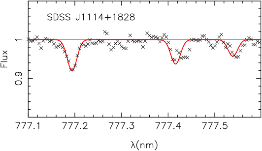
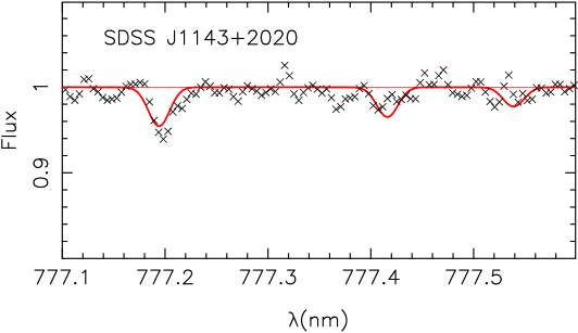
Figure 1: UVES spectrum in the region of the red O I  triplet.

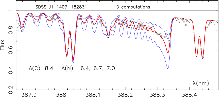
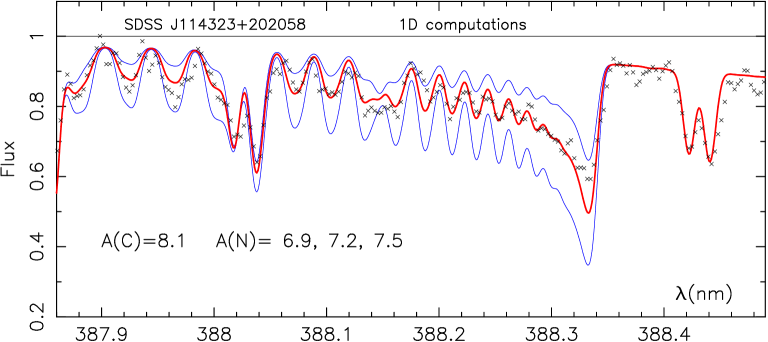
Figure 2: UVES spectrum in the region of the CN band compared to theoretical spectra. The abscissa is the wavelength in nm, and the ordinate the relative flux.
For SDSSJ1114+1828 the theoretical spectra are computed with A(C) = 8.4 and A(N) = 6.4, 6.7 (best fit), 7.0, and for SDSSJ1143+2020, with A(C) = 8.1 and A(N) = 6.9, 7.2 (best fit), 7.5.

The abundances of the light metals from sodium to calcium were corrected for NLTE effects following Andrievsky et al. (2007, 2008); Spite et al. (2012); Mashonkina (2013).

The green magnesium triplet (multiplet 2) is beyond the wavelength range of our spectra and thus we deduced the magnesium abundance from multiplet 3 (at 383 nm). Mashonkina (2013) has computed the NLTE correction for Mg taking into account inelastic collisions with neutral hydrogen atoms following Barklem et al. (2012). From her computations on a small grid of models, the NLTE correction for multiplet 3 amounts to about +0.14 dex for SDSSJ 1114+1828, 0.10 dex for SDSSJ 1143+2020 and 0.25 dex for SDSSJ 2209-0028.

The manganese abundances were derived by fitting synthetic spectra of the resonance lines (403 nm) to observations, taking into account the hyperfine structure of the lines. Cayrel et al., (2004) underlined that the manganese abundance deduced from the resonance lines was 0.4 dex lower (in giants) than the abundance deduced from the subordinate lines of Mn I. Moreover Bonifacio et al. (2009) have shown that there is a systematic difference between the ratio [Mn/Fe] in the turnoff stars and the giants even if only the resonance lines are taken into account. This behavior suggests a strong NLTE effect. The NLTE correction of the manganese abundance was computed for a grid of dwarf and subgiant models by Bergemann & Gehren (2008). Their most metal-poor model of turnoff star has a metallicity of -2.4 and for this metallicity the NLTE correction amounts to about +0.5 dex. This correction was applied to our LTE abundance.

Lai et al. (2008) and Bonifacio et al. (2009) have shown an offset between the chromium abundance derived from Cr I  and Cr II  lines in metal-poor stars, that points to NLTE effects. Bergemann & Cescutti (2010) have computed the NLTE correction for a set of Cr lines in metal-poor stars. The atmospheric parameters of one star (G 64-12) are close to those of our stars and thus we applied the NLTE correction found for the stronger resonance line of Cr I in G 64-12 (the only Cr line visible in our spectra): +0.44 dex.

The abundances of the heavy elements Sr and Ba are generally sensitive to NLTE effects. The abundance of Sr was corrected following Andrievsky et al. (2011). For Ba it has been shown (Andrievsky et al., 2009) that the NLTE correction depends almost only on [Ba/H] (the NLTE correction of the Ba lines is almost the same for two stars with different [Fe/H] but the same [Ba/H]). Since SDSS J1114+1828 and SDSS J1143+2020 are Ba-rich, [Ba/H] in these two stars is between –1.3 and –1.8 dex. For these values of [Ba/H], the NLTE correction, following Mashonkina et al. (1999), is close to zero (see their Table 4).

The line-by-line LTE abundances of the elements with the NLTE correction (when available) are given in Table Carbon-enhanced metal-poor stars: the most pristine objects? , and the resulting mean abundances are given in Table 4.

Table 4: Elemental abundances in the observed stars from a 1D analysis. Abundances of C(C I), O, Na, Mg, Al, Ca, Sr, and Ba have been corrected for NLTE effects (*), the LTE abundances for these elements are given line by line in Table Carbon-enhanced metal-poor stars: the most pristine objects? .

-		SDSS J111407.07+182831.7				SDSS J114323.42+202058.0				SDSS J220924.74-002859.8
model		6200, 4.0, –3.3, 1.3				6240, 4.0, –3.3, 1.3				6440, 4.0, –4.0, 1.3
Species	$\epsilon_{\odot}$	$\epsilon$	[M/H]	[M/Fe]	N	$\epsilon$	[M/H]	[M/Fe]	N	$\epsilon$	[M/H]	[M/Fe]	N
C(CH)	8.50	8.40	-0.10	3.25		8.10	-0.40	2.75		7.10	-1.40	2.56
C(C I)	8.50	7.95	-0.55	2.80	1	7.75	-0.75	2.40	1	-	-	-
N(CN)	7.86	6.70	-1.16	2.19		7.18	-0.68	2.47		-	-	-
O	8.76	7.31	-1.45	1.90	3	7.00	-1.76	1.39	3	6.97	-1.79	2.17	3
Na	6.30	4.58	-1.72	1.63	2	4.54	-1.76	1.39	2	$\leq 2.37$	$\leq-3.93$	$\leq 0.03$	2
Mg	7.54	5.65	-1.89	1.46	4	5.13	-2.41	0.74	4	4.30	-3.24	0.72	3
Al	6.47	3.48	-2.99	0.36	1	3.20	-3.27	-0.12	1	-	-	-
Ca	6.33	3.35	-2.98	0.37	6	3.49	-2.84	0.31	6	2.92	-3.41	0.55	5
Ti	4.90	1.86	-3.04	0.31	11	2.03	-2.87	0.28	11	-	-	-
Cr	5.64	2.49	-3.15	0.20	1	2.69	-2.95	-0.20	1	-	-	-
Mn	5.37	2.00	-3.37	-0.03	1	2.25	-3.12	0.03	1	-	-	-
Fe I	7.52	4.17	-3.35	0.00	36	4.37	-3.15	0.00	40	3.56	-3.96	0.0	6
Fe II	7.52	4.18	-3.34	0.00	3	4.24	-3.28	-0.13	3	-	-
Co	4.92	2.40	-2.52	0.83	3	2.26	-2.66	0.49	3	-	-	-
Ni	6.23	2.96	-3.27	0.07	2	2.98	-3.25	-0.10	2	-	-	-
Sr	2.92	0.29	-2.63	0.72	2	0.50	-2.42	0.73	2	$<-1.2$	$<-4.12$	$<-0.16$	1
Ba	2.17	0.44	-1.73	1.62	3	0.86	-1.31	1.84	3	$<-0.74$	$<-2.91$	$<+1.05$	1
Eu	0.52	$<-1.10$	$<-1.62$	$<1.73$	1	$<-1.00$	$<-1.52$	$<1.63$	1	-	-	-
$\rm[C/O]$			1.35				1.36				0.29
$\rm[Ba/Eu]$			$>0.1$				$>0.4$
$\rm{}^{12}C/^{13}C$			$>60$				$>20$

!

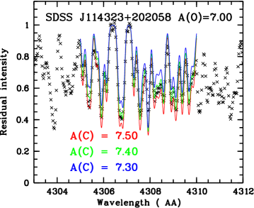
Figure 3: UVES spectrum of SDSS J114323+202058 in the core of the G band (black line), compared with two Linfor3D spectral syntheses with the CO⁵BOLD model, corresponding to A(C)=7.30, 7.40 and 7.50. The best fit is obtained with A(C)=7.40.

4.2 Effects of three-dimensional hydrodynamical convection on the formation of molecular bands

Classical models such as MARCS, have a number of simplifying assumptions: the atmosphere is approximated by a one-dimensional structure; all the physical quantities vary along the vertical direction, but are constant in the horizontal direction for any given depth; the atmosphere is supposed to be in hydrostatic equilibrium; all quantities are time independent; the stellar plasma is supposed to be in LTE, i.e. the particle velocities are given by a Maxwellian distribution at a local temperature $T$, the atomic populations are given by Boltzmann factors, at the same temperature $T$, ionization equilibria are also given by Saha’s law, at the same temperature. In cool stars convection is a hydrodynamical, time-dependent phenomenon, that needs to be treated in full three dimensional geometry. To treat these effects it is necessary to use hydrodynamical simulations, like those provided by the CO⁵BOLDcode (Freytag et al., 2012), which are fully hydrodynamical, time dependent, in a three dimensional frame, yet retaining the LTE assumption. In this investigation we concentrated on the hydrodynamical effects on molecular bands, because they have been shown to be extremely strong in metal-poor stars (Collet et al.,, 2007; Behara et al., 2010; González Hernández et al.,, 2010).

To estimate these effects we used a model extracted from the latest version of the CIFIST grid (Ludwig et al., 2009). The model has the parameters $\rm T_{eff}$/log g/[M/H] 6300/4.0/–3.0, and consists of a box of $140\times 140\times 150$ points, corresponding to physical dimensions $26\times 26\times 13$ Mm³. The opacity was derived from the MARCS suite (Gustafsson et al., 1975, 2003, 2008) and was binned into 12 opacity bins following the usual opacity binning scheme (Nordlund, 1983; Ludwig, 1992). Behara et al. (2010) noted a considerable difference between models computed with 6 opacity bins and those computed with 12 opacity bins.

The line formation in the three-dimensional structure was computed using Linfor3D. For the spectrum synthesis we used a selection of 20 snapshots, chosen to be statistically independent and representative of the overall characteristics of the hydrodynamical simulation. For comparison, Linfor3D also integrates the transfer equation through two reference one-dimensional structures:
– an $\mathrm{1D}_{\mathrm{LHD}}$ model (see Caffau & Ludwig, 2007) that uses the same microphysics as CO⁵BOLD; and
– a $\left\langle\mathrm{3D}\right\rangle$  model, that is obtained by averaging the three dimensional structure over surfaces of constant Rosseland optical depth and over time.

Following Caffau & Ludwig (2007), we defined the 3D correction as the difference in the abundance derived from the full 3D synthesis and that derived from the $\mathrm{1D}_{\mathrm{LHD}}$ model (3D – $\mathrm{1D}_{\mathrm{LHD}}$). It is also useful to consider the difference between the abundance derived from the 3D model and the $\left\langle\mathrm{3D}\right\rangle$ model. Since the two models have by construction the same mean temperature distribution, this difference helps to single out the effect of temperature fluctuations.

Computing molecular bands is CPU-intensive, since many lines need to be treated. The G-band is very challenging since it extends over almost 20 nm. The data for the G-band (CH AX electronic system) were taken from Plez & Cohen, (2005) and Plez et al. (2008). We computed the full 3D synthesis of the G band core for various carbon abundances and compared them with the observed spectrum. The result for SDSS J114323+202058 is shown in Fig.3. The best fit is obtained for A(C)=7.4 and as a consequence, the 1D to 3D correction is about -0.7 dex.

For the nitrogen abundance we used the CN BX [ B${}^{2}\Sigma^{+}$ –X${}^{2}\Sigma^{+}$ (0–0) ] violet band at 388 nm. We used the molecular data from Hill et al. (2002) and Plez et al. (2008), but considering the limited spectral range covered by the band (about 0.5 nm), it is feasible to synthetise the whole band, as shown in Fig. 4. The 3D effect seems to be much more important for this band than for the CH band. This band is formed very close to the surface of the star and the nitrogen abundance deduced from this band is also strongly affected by the quantity of oxygen atoms bound at this level in the CO molecule. As a consequence, we found for these oxygen-rich stars, a huge correction: about –2.4 dex. This correction (if confirmed) would almost annihilate the nitrogen enhancement in the CEMP turnoff stars. These 3D corrections affect not only the three turnoff stars we studied but all CEMP stars in the literature where these 3D effects have generally been neglected. These effects could be so significant that they could lead to a revision of the interpretation of the abundances in these stars (type of AGB stars responsible for the abundance anomalies). In Figure 4 we compare the 1D and the 3D profiles of the CN band in SDSS J1143+2020 with different abundances.

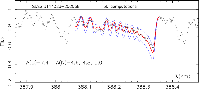
Figure 4: UVES spectrum in the region of the CN band of SDSS J1143+2020. The abscissa is the wavelength in nm, and the ordinate is the relative flux.
In the top panel the observed spectrum (crosses) is compared to 1D theoretical spectra computed with A(C) = 8.1 (best fit for the CH band in 1D) and A(N) = 6.9, 7.2 (best fit), 7.5.
In the bottom panel the observed spectrum is compared to 3D theoretical spectra computed with A(C) = 7.4 (best fit for the CH band in 3D, see Fig. 3) and A(N)= 4.6, 4.8 (best fit) and 5.0.

To confirm this very large correction of the nitrogen abundance, it would be very important to compare the abundance deduced from the CN band and from the NH band, which is practically independent of the oxygen abundance. But the NH band is not in the observed spectral range of the very faint stars studied in the present paper. We will study this effect, which is very sensitive to the most external layers of the models, in another sample of CEMP stars with known CN and NH bands in a future investigation.

Since the aim of the present paper is to enlarge the sample of the abundance patterns in CEMP stars, we discuss in the remainder of this paper the 1D abundances to facilitate a comparison with the previous analyses, but with the caveat that the abundance of C and N could be strongly reduced.

4.3 SDSS J1114 +1828 and SDSS J1143+2020

Both stars are very metal-poor ($\rm[Fe/H]<-3.0$) and exhibit a very strong enhancement of C, N, O and Mg (Table 4). This enhancement tends to decrease with the atomic number. The CN feature is displayed in Fig. 2.

The carbon abundance deduced from the C I line is systematically lower by about 0.4 dex than the abundance deduced from the CH band. This difference has also been observed by Behara et al. (2010). A 3D computation of the CH band and the C I lines does not remove this discrepancy, but in this case the abundance of C derived from the C I line is higher than the abundance derived from the CH band. Since in the literature the carbon abundance is generally deduced from 1D computation of the CH band we used the C (CH) abundance in the forthcoming discussion.

The overabundance of C, N, and O in these stars is generally attributed to a production in an AGB companion that transfers some processed material to the observed star. This hypothesis is reinforced by the fact that the radial velocity of both stars have been found to be variable in section 3. In Figure 5 we plot these two new CEMP turnoff stars in a diagram [N/Fe] vs. [C/Fe] for comparison with the values found for other CEMP dwarfs and turnoff stars (Sivarani et al., 2006; Behara et al., 2010; Masseron et al., 2012) and the predictions of Herwig et al. (2004) computed for AGB stars with $6M_{\odot}$ HBB (Hot Bottom Burning model) and $2M_{\odot}$ non-HBB. Like most of the CEMP turnoff stars, SDSS J111407+182831 and SDSS J1143+2020 lie in the region delimited by these two models (see Sivarani et al., 2006).

However, we must have in mind that in a 3D analysis all stars in this graph would have to be shifted toward lower values of [C/Fe] (–0.5 dex) and mainly much lower values of [N/Fe]. This will be discussed in a follow-up paper.

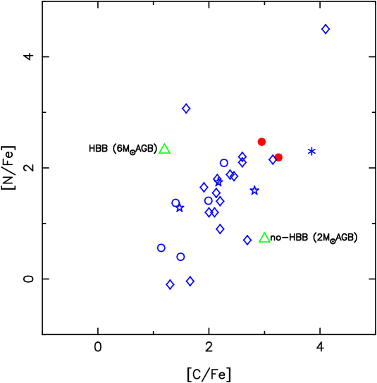
Figure 5: [N/Fe] vs. [C/Fe] for CEMP dwarfs and turnoff stars from the recent literature (Sivarani et al., 2006,  diamonds), (Behara et al., 2010,  stars), (Masseron et al., 2012,  open circles), (Christlieb et al.,, 2002,  asterisk), and for our stars SDSS J111407+182831 and SDSS J1143+2020 (filled circles). The AGB models predicted by Herwig et al. (2004), for [Fe/H]=–2.3 and initial masses $6M_{\odot}$ (HBB) and $2M_{\odot}$ (non-HBB) are labeled by triangles.

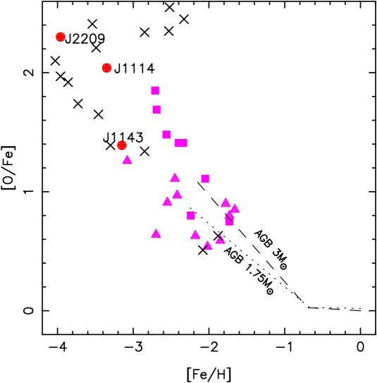
Figure 6: [O/Fe] vs. [[Fe/H]] for CEMP-s stars (triangles), CEMP-rs stars (squares), CEMP-no stars (crosses) following Masseron et al. (2010). Our stars are represented by red full circles. The predictions of Karakas & Lattanzio (2007) for pollution by $1.75M_{\odot}$ and $3M_{\odot}$ AGB are indicated as dotted and dashed lines.

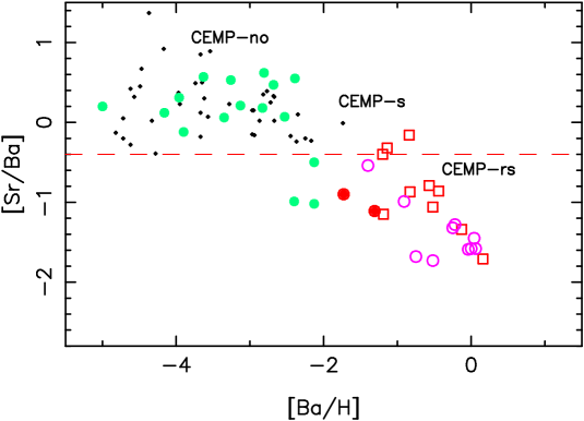
Figure 7: [Sr/Ba] vs. [Ba/H] for normal metal-poor stars (black dots) following (Andrievsky et al., 2011), and CEMP stars following Frebel (2010) and Cescutti & Chiappini (2013). Green filled circles represent CMP-no stars, open red squares CMP-s stars, and open magenta circles CMP-rs stars. The red dots represent SDSS J111407+182831 and SDSS J1143+2020. In case of mass transfer from an AGB companion $\rm[Sr/Ba]<-0.4$ (dashed line). Our stars fulfill this requirement.

4.3.1 Heavy elements Sr, Ba, Pb, and class determination of the stars

With a Ba overabundance $\rm[Ba/Fe]>1.0$, the two stars SDSS J111407+182831 and SDSS J1143+2020 belong (Beers & Christlieb, 2005), to the class of the CEMP-s stars or to the CEMP-rs stars, depending on the abundance of Eu ($\rm[Ba/Eu]>0.5$ in CEMP-s stars and $\rm 0.0<[Ba/Eu]<0.5$ in CEMP-rs stars). The europium line is not visible in these two CEMP turnoff stars, and the low S/N of the spectra in the region of the main Europium line (412.9 nm) does not allow a very restrictive estimate of the Eu abundance.

Masseron et al. (2010) have proposed a classification based on [Ba/Fe] alone, when [Eu/Fe] is not available. From their Figure 1, the stars are all CEMP-rs when $\rm[Ba/Fe]>2.1$. But when $\rm 1.6<[Ba/Fe]<1.9$ like in our stars, there is about the same number of CEMP-s and CEMP-rs stars.

On the other hand, Masseron et al. (2010) have shown that, for the same metallicity, the CEMP-rs stars have a higher value of [O/Fe] than the CEMP-s stars. In Fig. 6 we have plotted [O/Fe] vs. [Fe/H] for the stars of Masseron et al. (2010), with $\rm[Fe/H]<-1.5$ (their Fig. 18) and for our stars; the dashed and dotted lines in this figure represent the predictions of Karakas & Lattanzio (2007) for AGB of $1.75M_{\odot}$ and $3M_{\odot}$. This graph supports the idea that CEMP-rs stars have been polluted by stars with a higher mass AGB than CEMP-s stars (Masseron et al., 2010) and that SDSS J111407+182831 with its very high oxygen abundance could be classified as a CEMP-rs, and SDSS J1143+2020 as a CEMP-s star.

In Fig. 7 we have plotted [Sr/Ba] as a function of [Ba/H] for different types of CEMP stars. The abundances of Sr and Ba have been taken from Frebel (2010). All CMP-s and CMP-rs stars have a known Europium abundance. We adopted the definitions of Sivarani et al. (2006): we called CEMP-no stars all CEMP stars with $\rm[Ba/Fe]<1.0$ (CEMP-no or CEMP-low-s), the CEMP-s and CEMP-rs stars have $\rm[Ba/Fe]>1.0$ with $\rm[Ba/Eu]>0.5$ for the CEMP-s and $\rm 0<[Ba/Eu]<0.5$ for the CEMP-rs stars. The small dots represent the “normal” EMP stars (Andrievsky et al., 2011). The ratio [Sr/Ba] in the CEMP-s and CEMP-rs stars is much lower than in the classical EMP stars. This low ratio is generally compatible with a mass transfer from an AGB companion $\rm([Sr/Ba]<-0.4$). In this figure, both SDSS J111407+182831 and SDSS J1143+2020 are located in the region corresponding to both the CEMP-s and CEMP-rs stars, their abundances of Sr and Ba are compatible with a mass transfer from an AGB (unlike the majority of the CEMP-no stars).

Following Masseron et al. (2010), when $\rm[Fe/H]<-3.0$, the CEMP-no stars ($\rm[Ba/Fe]<+1.0$) are much more numerous than the CEMP-s or CEMP-rs stars. These authors note that neither CEMP-rs nor CEMP-s stars have been discovered below $\rm[Fe/H]<-3.2$. Thus SDSS J111407+182831 with [Fe/H]=–3.35 is to date the most metal-poor CEMP-s or CEMP-rs star.

Several carbon-rich stars CEMP-s and CEMP-rs stars are also lead-rich (see e.g.: Cohen et al., (2003), Barbuy et al. (2005), Bisterzo et al. (2006)). We tried to detect Pb in SDSS J1114 +1828 and SDSS J1143+2020 (Fig. 8). The best fits were obtained with $\rm A(Pb)=1.6\pm 0.3$ for SDSS J1114+1828, and $\rm A(Pb)=1.8\pm 0.2$ for SDSS J1143+2020. The corresponding equivalent widths are respectively about 4 and 6 mÅ. In this region of the spectrum the S/N is around 50 (see Table 2), therefore from the Cayrel (1988) formula, the error on the equivalent width is lower than 2mÅ. For SDSS J1143+2020 the detection of Pb is highly significant ($>95\%$). In both stars $\rm[Pb/Fe]\approx+3.0$, a value very close to the values of [Pb/Fe] generally found from LTE computations in similar stars (Bisterzo et al., 2006). But the Pb abundance has to be corrected for NLTE effects which, following Mashonkina et al. (2012), are strong in metal-poor stars. These authors have not computed the correction for turnoff stars with a metallicity as low as those of SDSS J1114+1828 and SDSS J1143+2020, but since the correction increases with the temperature and with decreasing metallicity, it is at least equal to +0.3 according to their Table 1,

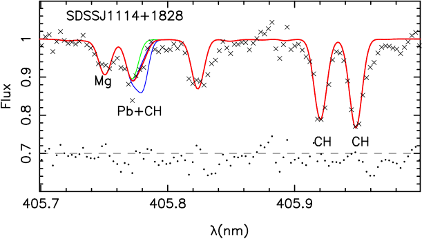
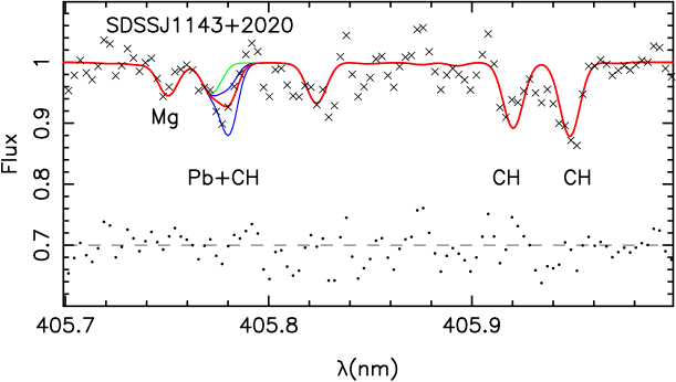
Figure 8: Spectra of SDSS J1114+1828 and SDSS J1143+2020 in the region of the Pb line. The synthetic spectra have been computed without Pb (green line) and with A(Pb)= 1.5 and 2.1 (thin blue lines). The best fits (red lines) are obtained with A(Pb)=1.6 for SDSS J1114+1828 and A(Pb)=1.8 for SDSS J1143+2020.

4.3.2 $\rm{}^{12}C/^{13}C$ ratio

The $\rm{}^{13}C$ features are not visible in the observed spectra (Fig.9). We deduced lower limits: $\rm{}^{12}C/^{13}C\geq 60$ for SDSS J111407+182831 and $\rm{}^{12}C/^{13}C\geq 22$ for SDSS J1143+2020. An example of the $\rm{}^{13}C$ feature is displayed in Fig. 9. These lower limits are compatible with the values found in the CEMP-s and CEMP-rs stars (see Masseron et al., 2010, their Fig.17). Masseron et al. (2010) have remarked that, although the mechanism responsible for the N production may be attributed to CBB (cool bottom burning) in the framework of AGB evolution, no current AGB models reproduce the observed trend of $\rm\log^{12}C/^{13}C$ vs. [C/N].

Figure 9: UVES spectrum in the region of the CH band in SDSS J111407+182831 compared to theoretical spectra computed with $\rm A(^{12}C{)}$=8.4 and $\rm{}^{12}C/^{13}C$ equal to either 10 (thin blue line) or 60 (thick red line). The abscissa is the wavelength in nm, and the ordinate the relative flux. The $\rm{}^{13}C$ feature is not visible in the observed spectrum, and we derived for this star $\rm{}^{12}C/^{13}C\geq 60$.

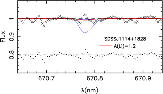
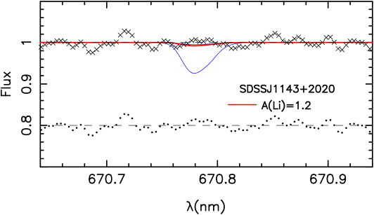
Figure 10: UVES spectrum in the region of the lithium feature. The thin blue line corresponds to the lithium feature computed with the classical abundance A(Li)= 2.2, and the thick red line to the best fit (A(Li)=1.2 in both cases). The dots at the bottom of the figures represent the difference between this best fit and the observed spectrum (shifted upward by 0.8). We adopted in both cases $\rm A(Li)<1.5$.

4.3.3 Lithium abundance

In normal (non C-enhanced) turnoff stars with a metallicity higher than $\rm[Fe/H]=-3.0$, the lithium abundance A(Li) is generally constant, independent of the temperature and metallicity and equal to about 2.2 dex defining a plateau (see e.g. Spite et al., 2012). But below $\rm[Fe/H]=-3.0$ there is a meltdown of the plateau (e.g. Bonifacio et al., 2007; González Hernández et al., 2008; Sbordone et al., 2010) and a large part of the normal very deficient stars have a lithium abundance lower than 2.2.

In the CEMP turnoff stars, even with a metallicity higher than $\rm[Fe/H]=-3.0$, the lithium abundance is often lower than the value of the plateau. In the spectra of SDSS J1114+1828 and SDSS J1143+2020 the lithium line is not visible (Fig. 10). We derived in both cases $\rm A(Li)\leq 1.5$, a lithium abundance well below the value of the plateau.

The low abundance of Li in CEMP (s and rs) stars is discussed by Masseron et al. (2012). Briefly, before the transfer of material from the AGB companion, the lithium abundance in the observed star should be the same as in normal metal-poor turnoff stars, but as more and more AGB material is transferred to the atmosphere of the star, the carbon abundance increases while the lithium abundance decreases because in most cases the lithium abundance in the AGB star is lower than the lithium plateau.

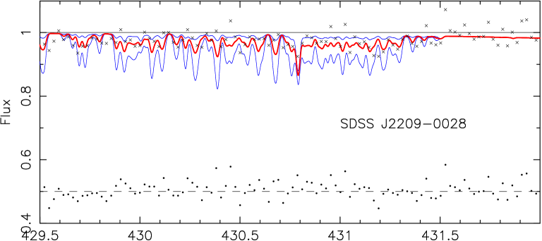
Figure 11: UVES spectrum in the region of the CH band in SDSS J2209-0028. The thin blue lines correspond to the computation of the CH band with an abundance A(C)=6.5 and 7.5. The thick red line corresponds to A(C)=7.1 (best fit) and the dots at the bottom of the figure represent the difference between the synthetic spectrum computed with A(C)=7.1 and the observed spectrum (shifted upward by 0.5).

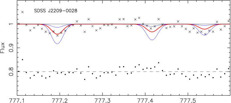
Figure 12: Thin blue lines correspond to synthetic spectra computed with A(O)= 6.5 and 7.5. and the thick red line (best fit) has been obtained with A(O)=7.1. The crosses represent the observed spectrum (binned x2) and the dots at the bottom of the figure are the difference between the best fit and the observed spectrum (shifted upward by 0.8).

4.4 SDSS J220924-002859

SDSS J220924-002859 with $\rm[Fe/H]\approx-4$ is the most metal-poor star of our sample. Compared to the other two stars its carbon abundance is also ten times lower. But it is also the faintest star of our sample (Table 1) and the S/N of the spectra is much lower (Table 2). As a consequence the abundance of only few elements could be measured in this star.

The 1D carbon abundance in SDSS J220924-002859 was estimated to be $\rm A(C)=7.0\pm 0.2dex$ (Fig 11), with the 3D correction we derived $\rm A(C)=6.5\pm 0.2dex$. However, we remark that the S/N in this star is so poor that the CH band in the spectrum is at the limit of the detection and it would be very interesting to obtain a new better spectrum in this region.

With [O/Fe]=2.10, SDSS J220924-002859 is the most oxygen-rich star in our sample (Fig. 12). The barium line is not visible in our spectrum and we derived, within the LTE hypothesis, an upper limit $\rm[Ba/Fe]<0.75$ (this upper limit becomes $\rm[Ba/Fe]<1.05$ when the NLTE effects are taken into account). It should thus belong to the CEMP-no stars (defined by $\rm[Ba/Fe]_{LTE}<+1$ see also the Fig. 7).

The star is very oxygen-rich, and in Fig. 6 it indeed appears in the region of the CEMP-no stars. SDSS J220924-002859 belongs to this class, as do most of the extremely iron-poor carbon-rich stars (Masseron et al., 2010).

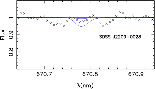
Figure 13: UVES spectrum in the region of the lithium feature. The thin blue lines correspond to the lithium feature computed with the abundance A(Li)=1.2 and 2.2. The noise is important in this region of the spectrum and therefore we derive $\rm A(Li)\leq 2.2$.

In SDSS J220924-002859 the best fit is obtained with $\rm A(Li)=1.8\pm 0.4$ (Fig. 13). The noise is very high in this region of the spectrum and the abundance of the plateau A(Li)=2.2 cannot be excluded.

5 Discussion and Conclusion

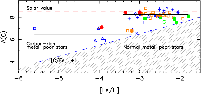
Figure 14: Abundance of carbon A(C) vs. [Fe/H] in dwarfs and turnoff CEMP stars, following Sivarani et al. (2006, their Table 4), [orange open squares]), Frebel et al. (2005, 2007) [blue open squares], Thompson et al. (2008) [green open circle], Aoki et al. (2009) [blue open diamonds], Behara et al. (2010) [full orange circles], Placco et al. (2011) [blue $\times$), Carollo et al., (2011) [blue $+$], Masseron et al. (2010, 2012) [full green squares], Yong et al. (2013b) [blue open triangles]. Our measurements are represented with full red circles. The dashed blue line (representing $\rm[C/Fe]=+1$) separates the region of the carbon-rich metal-poor stars from the region of the normal metal-poor stars (hatched). When [Fe/H] is higher than –3 the carbon abundance is almost constant and close to 8.25 (see also Masseron et al., 2010). For $\rm[Fe/H]<-3.4$ the carbon abundance drops suddenly to about 6.5. However, it is difficult to decide whether at very low metallicity A(C) is also constant, or whether the line A(C)=6.5 represents an upper limit of the carbon abundance in these extremely metal-poor star (Masseron et al., 2010).

In Fig.14 we plotted the recent measurements of the abundance of C in CEMP dwarf and turnoff stars as a function of [Fe/H], for $\rm[Fe/H]<-1.8$ collecting the data of Sivarani et al. (2006, their Table 4), Frebel et al. (2005, 2007), Thompson et al. (2008), Aoki et al. (2009), Behara et al. (2010), Placco et al. (2011), Carollo et al., (2011), Masseron et al. (2010, 2012) Yong et al. (2013b), and this paper. We did not considered the giants because their carbon abundance can be affected by mixing with deep layers (see e.g., at low metallicity, Spite et al., 2005, 2006). In this figure we have kept the carbon abundance deduced from the CH molecular band and 1D computations to facilitate the comparison with the results in the literature since generally these previous abundances were derived from this feature and from 1D models. All stars in the graph are turnoff stars or dwarfs, the 3D correction must be about the same for all these stars, and, after this correction, the global view should remain similar.

According to the definition of the carbon-rich metal-poor stars ($\rm[C/Fe]>+1$) these stars are located above the dashed blue line in Fig. 14. From this figure it seems that for $\rm[Fe/H]>-3$ the logarithm of the carbon abundance A(C) is almost constant close to 8.25, a value slightly lower than the solar value (A(C)=8.5). This can reflect the fact that the carbon quantity transferred by the defunct AGB companion to the observed carbon-rich metal-poor star, has been such as to reach the same total amount in all stars, whatever the metallicity between –1.8 and –3 (see Masseron et al., 2010).

The carbon abundance is clearly lower, with $\rm A(C)\approx 6.8$ for the low metallicities ($\rm[Fe/H]<-3.4$). None of these stars have a (1D) carbon abundance significantly higher than A(C)=7.0. However, the number of carbon-rich metal-poor stars with $\rm[Fe/H]<-3.4$ is very small and it is not possible to decide wether the mean value A(C)=6.8 represents a plateau of the carbon abundance or if it is an upper limit. Moreover, in this metallicity range, the stars are generally faint and a precise determination of the carbon abundance below A(C)=7.0 is difficult in turnoff stars. It would be interesting to find more CEMP dwarf stars with a temperature below 6000K and consequently a stronger CH absorption band, to reach a better determination of the behavior of the carbon abundance in the extremely metal-poor carbon stars.

In all stars with $\rm[Fe/H]<-3.4$, the barium abundance is also rather low: $\rm[Ba/Fe]<1.0$. All these stars belong to the class of the CEMP-no stars. Five other stars are located close to this plateau but with a metallicity higher than $\rm[Fe/H]=-3.4$. In two of them (studied from high-resolution spectra) the abundance of Ba was measured. In BPS CS 29528-041, [Ba/Fe] is lower than 1.0. Therefore, this star belongs to the CEMP-no stars (Sivarani et al., 2006), but SDSS J1036+1212 (Behara et al., 2010) is Ba-rich ($\rm[Ba/Fe]=1.17$) and has a ratio $\rm[Eu/Fe]=1.26$. In this star $\rm[Ba/Eu]=-0.09$, this value is very close to $\rm[Ba/Eu]=0.0$ (within the error bar) and thus SDSS J1036+1212 is probably a CEMP-rs star (see also the Fig.1 of Masseron et al., 2010).

The cause of the abundance anomalies of the CEMP-no stars are currently only poorly understood. An enrichment in only C, N, and O by AGBs has been proposed (Masseron et al., 2010), but in this case we would expect that many CEMP-no stars are binaries : only one CEMP-no star is known to be a binary (Preston & Sneden, 2001), and the radial velocity of SDSS J220924-002859 seems to be stable between 2003 and 2011 (see section 3). However, more radial velocity measurements over a longer period of time would be necessary to exclude binarity. The abundance pattern of the CEMP-no stars could be also the result of a pre-enrichment of the interstellar medium by e.g. faint supernovae associated with the first generations of stars (Umeda et al., 2003, 2005; Tominaga et al., 2007), or by C-rich winds of massive rotating EMP stars (Hirschi et al.,, 2006; Meynet et al., 2006).

To better interpret the abundance pattern of the CEMP-no stars, it is important to clearly establish wether the carbon abundance in this type of star is constant at a level of $\rm A(C)\approx 6.8$ or wether this value is only an upper limit of the carbon abundance. It would be very important to significantly enlarge the sample of the abundance pattern of the very metal-poor CEMP stars and to study the scatter around the upper plateau, as well as around the possible lower plateau. Monitoring the radial velocities of the CEMP-no stars would also be important to research of the origin of the CEMP stars.

A 3D analysis of the CH and CN bands suggests that in metal-poor turnoff stars the carbon abundance could be 0.7 dex lower and the nitrogen abundance 2.4 dex lower than those derived in a 1D analysis of the CH G band or the CN band. This effect, which strongly depends on the external layers of the models, will be studied in detail in a forthcoming paper.

longtable—lcrr—rrr—rrr—rrr— Linelist equivalent widths and abundances
  SDSS J111407+182831    SDSS J114323+202058    SDSS J220924-002859  
Elem $\lambda$Exc.Pot.$\log gf$ EW abund abund EW abund abund EW abund abund
(Å) (eV) (mÅ) LTE NLTE (mÅ) LTE NLTE (mÅ) LTE NLTE
continued.
  SDSS J111407+182831    SDSS J114323+202058    SDSS J220924-002859  
Elem $\lambda$Exc.Pot.$\log gf$ EW abund abund EW abund abund EW abund abund
(Å) (eV) (mÅ) LTE NLTE (mÅ) LTE NLTE (mÅ) LTE NLTE
C 1 4932.049 7.69 -1.884 syn 8.40 7.97 syn 8.20 7.77

O 1 7771.941 9.15 0.369 syn syn 7.20 7.07 syn 7.10 6.97
O 1 7774.161 9.15 0.223 syn 7.45 7.31 syn 6.90 6.82 syn 7.10 6.97
O 1 7775.388 9.15 0.001 syn

Na 1 5889.951 0.00 0.117 149.8 4.67 4.57 142.6 4.63 4.53
Na 1 5895.924 0.00 -0.184 127.2 4.69 4.59 122.0 4.66 4.56

Mg 1 3829.355 2.71 -0.231 syn 5.35 5.49 syn 4.90 5.00 syn 3.65 3.90
Mg 1 3832.304 2.71 0.146 syn 5.50 5.64 syn 5.05 5.15 syn 3.95 4.20
Mg 1 3838.290 2.72 0.415 syn 5.55 5.69 syn 5.05 5.15 syn 3.95 4.20
Mg 1 4702.991 4.35 -0.666 39.3 5.64 5.78 14.5 5.11 5.21

Al 1 3961.520 0.01 -0.323 48.0 2.83 3.48 31.5 2.55 3.20

Ca 1 4226.728 0.00 0.244 81.2 3.30 3.42 87.8 3.49 3.64 42.1 2.60 2.82
Ca 1 4454.779 1.90 0.258 17.2 3.57 3.70 16.7 3.54 3.70
Ca 1 6162.173 1.90 -0.090 5.4 3.25 3.43 13.6 3.71 3.89
Ca 2 3933.680 0.00 0.105 syn 3.45 3.44 syn 3.55 3.55 syn 2.85 2.82
Ca 2 8498.023 1.69 -1.416 118.2 3.65 3.30 133.0 3.87 3.55 92.6 3.35 3.05
Ca 2 8542.091 1.70 -0.463 206.4 3.50 2.99 250.0 3.74 3.19 180.6 3.47 2.87
Ca 2 8662.170 1.69 -0.723 211.3 3.76 3.24 215.0 3.82 3.29 134.5 3.36 2.81

Sc 2 4246.822 0.31 0.242 47.2 0.71 25.7 0.27

Ti 1 4981.731 0.85 0.504 syn 2.1
Ti 2 3759.291 0.61 0.280 syn 1.7 70.4 2.03
Ti 2 3761.320 0.57 0.180 syn 1.7 67.4 2.02
Ti 2 3913.461 1.12 -0.420 16.0 1.81 20.0 1.95
Ti 2 4417.714 1.16 -1.190 syn 2.1 5.2 2.05
Ti 2 4443.794 1.08 -0.720 12.4 1.90 17.1 2.08
Ti 2 4450.482 1.08 -1.520 syn 2.0 5.1 2.29
Ti 2 4464.449 1.16 -1.810 4.3 2.57
Ti 2 4468.507 1.13 -0.600 19.1 2.05 14.7 1.93
Ti 2 4501.270 1.12 -0.770 10.3 1.88 10.1 1.89
Ti 2 4533.960 1.24 -0.530 syn 1.75 19.1 2.09
Ti 2 4563.757 1.22 -0.690 8.4 1.80 8.1 1.80
Ti 2 4571.968 1.57 -0.320 syn 1.8 20.4 2.23

V 1 4379.230 0.30 0.580 10.8 2.25

Cr 1 4254.336 0.00 -0.114 syn 2.05 2.49 22.1 2.25 2.69

Mn 1 4030.753 0.00 -0.470 2.00 syn 1.95
Mn 1 4033.062 0.00 -0.618 syn 1.50 2.00 syn 1.85

Fe 1 3758.233 0.96 -0.027 69.0 4.05 78.8 4.37
Fe 1 3763.789 0.99 -0.238 51.9 3.80 72.2 4.42
Fe 1 3767.192 1.01 -0.389 54.2 4.03 59.7 4.22
Fe 1 3786.677 1.01 -2.225 7.6 4.51 8.1 4.58
Fe 1 3787.880 1.01 -0.859 35.4 4.04 45.5 4.31
Fe 1 3815.840 1.49 0.237 61.6 4.03 73.5 4.40
Fe 1 3820.425 0.86 0.119 86.2 4.26 93.3 4.48
Fe 1 3824.444 0.00 -1.362 62.1 4.29 66.0 4.45
Fe 1 3827.822 1.56 0.062 52.6 4.03 54.4 4.11
Fe 1 3840.437 0.99 -0.506 54.3 4.12 67.2 4.51
Fe 1 3849.966 1.01 -0.871 46.4 4.30 53.6 4.52
Fe 1 3850.818 0.99 -1.734 16.7 4.40 20.4 4.55
Fe 1 3856.371 0.05 -1.286 63.3 4.29 67.3 4.46
Fe 1 3859.911 0.00 -0.710 75.3 4.04 81.7 4.28
Fe 1 3865.523 1.01 -0.982 34.0 4.12 54.6 4.65
Fe 1 3878.018 0.96 -0.914 45.8 4.27 55.5 4.56
Fe 1 3899.707 0.09 -1.531 55.1 4.32 58.5 4.46
Fe 1 3920.258 0.12 -1.746 38.2 4.14 49.0 4.44
Fe 1 3922.912 0.05 -1.651 43.7 4.11 50.4 4.32
Fe 1 4005.242 1.56 -0.610 29.3 4.13 33.8 4.27
Fe 1 4045.812 1.49 0.280 64.6 4.03 69.1 4.19 36.4 3.52
Fe 1 4063.594 1.56 0.062 60.8 4.20 64.2 4.33 31.7 3.69
Fe 1 4071.738 1.61 -0.022 46.9 3.98 57.7 4.29 28.9 3.75
Fe 1 4076.629 3.21 -0.529 10.5 4.97
Fe 1 4132.058 1.61 -0.675 28.1 4.20 24.8 4.15
Fe 1 4143.868 1.56 -0.511 35.1 4.15 33.0 4.13
Fe 1 4157.780 3.42 -0.403 26.6 5.54 14.9 5.22
Fe 1 4199.095 3.05 0.155 44.6 5.07 39.9 4.99
Fe 1 4202.029 1.49 -0.708 24.5 4.02 34.8 4.30
Fe 1 4222.213 2.45 -0.967 9.5 4.68
Fe 1 4227.427 3.33 0.266 13.9 4.41 17.4 4.56
Fe 1 4250.119 2.47 -0.405 16.1 4.37 11.0 4.20
Fe 1 4260.474 2.40 0.109 26.5 4.09 26.5 4.11
Fe 1 4383.545 1.49 0.200 64.4 4.05 67.6 4.18 28.8 3.39
Fe 1 4404.750 1.56 -0.142 41.9 3.91 52.3 4.18 17.4 3.49
Fe 1 4443.194 2.86 -1.043 5.1 4.79 5.2 4.82
Fe 1 4466.551 2.83 -0.600 7.4 4.50 7.5 4.53
Fe 1 4489.739 0.12 -3.966 8.6 5.41 4.9 5.19
Fe 1 4528.614 2.18 -0.822 10.4 4.28 13.8 4.45
Fe 1 4531.148 1.49 -2.155 5.5 4.66 4.3 4.58
Fe 1 4891.492 2.85 -0.112 16.5 4.40
Fe 1 4918.994 2.87 -0.342 11.7 4.49
Fe 1 4920.502 2.83 0.068 11.3 4.01 18.5 4.29
Fe 2 4233.172 2.58 -1.947 8.2 4.23 7.7 4.20
Fe 2 4583.837 2.81 -1.867 5.3 4.12 8.7 4.37
Fe 2 4923.927 2.89 -1.320 16.0 4.18 15.0 4.15

Co 1 3845.461 0.92 0.010 16.5 2.46 syn 2.3
Co 1 3995.302 0.92 -0.220 10.0 2.41 syn 2.2
Co 1 4121.311 0.92 -0.320 7.3 2.34 6.0 2.29

Ni 1 3807.138 0.42 -1.205 15.1 2.96 syn 3.12
Ni 1 3858.292 0.42 -0.936 23.8 2.95 syn 2.85

Zn 1 4810.528 4.08 -0.137 2.5 2.09 2.7 2.14

Sr 2 4077.709 0.00 0.167 64.4 0.11 0.31 70.9 0.34 0.54 $<8.0$ $<-1.45$$<-1.20$
Sr 2 4215.519 0.00 -0.145 53.5 0.06 0.26 59.3 0.26 0.46

Ba 2 4554.029 0.00 0.170 syn 0.41 0.41 syn 0.95 0.95 $<10.0$ $<-1.04$$<-1.04$
Ba 2 5853.668 0.60 -1.000 syn 0.80 0.80
Ba 2 6141.713 0.70 -0.076 36.6 0.42 0.42 52.5 0.85 0.85
Ba 2 6496.897 0.60 -0.377 32.0 0.50 0.50 44.6 0.83 0.83