Revisiting the Nyström method for improved large-scale machine learning

Abstract.

We reconsider randomized algorithms for the low-rank approximation of symmetric positive semi-definite (SPSD) matrices such as Laplacian and kernel matrices that arise in data analysis and machine learning applications. Our main results consist of an empirical evaluation of the performance quality and running time of sampling and projection methods on a diverse suite of SPSD matrices. Our results highlight complementary aspects of sampling versus projection methods; they characterize the effects of common data preprocessing steps on the performance of these algorithms; and they point to important differences between uniform sampling and nonuniform sampling methods based on leverage scores. In addition, our empirical results illustrate that existing theory is so weak that it does not provide even a qualitative guide to practice. Thus, we complement our empirical results with a suite of worst-case theoretical bounds for both random sampling and random projection methods. These bounds are qualitatively superior to existing bounds—e.g., improved additive-error bounds for spectral and Frobenius norm error and relative-error bounds for trace norm error—and they point to future directions to make these algorithms useful in even larger-scale machine learning applications.

1. Introduction

inline]Use a remark environment for numbering and better formatting of the remarks inline]Talwalkar: References [36] and [57] are often mixed up during citations, e.g., on page 2 (last paragraph), page 5 (above equation 5 and below equation 6). In particular, [57] provides coherence-based bounds for the Nystrom method in the low-rank setting.

We reconsider randomized algorithms for the low-rank approximation of symmetric positive semi-definite (SPSD) matrices such as Laplacian and kernel matrices that arise in data analysis and machine learning applications. Our goal is to obtain an improved understanding, both empirically and theoretically, of the complementary strengths of sampling versus projection methods on realistic data. Our main results consist of an empirical evaluation of the performance quality and running time of sampling and projection methods on a diverse suite of dense and sparse SPSD matrices drawn both from machine learning as well as more general data analysis applications. These results are not intended to be comprehensive but instead to be illustrative of how randomized algorithms for the low-rank approximation of SPSD matrices behave in a broad range of realistic machine learning and data analysis applications.

In addition to being of interest in their own right, our empirical results point to several directions that are not explained well by existing theory. (For example, that the results are much better than existing worst-case theory would suggest, and that sampling with respect to the statistical leverage scores leads to results that are complementary to those achieved by projection-based methods.) Thus, we complement our empirical results with a suite of worst-case theoretical bounds for both random sampling and random projection methods. These bounds are qualitatively superior to existing bounds—e.g., improved additive-error bounds for spectral and Frobenius norm error and relative-error bounds for trace norm error. Importantly, by considering random sampling and random projection algorithms on an equal footing, we identify within our analysis deterministic structural properties of the input data and sampling/projection methods that are responsible for high-quality low-rank approximation.

In more detail, our main contributions are fourfold.

• First, we provide an empirical illustration of the complementary strengths and weaknesses of data-independent random projection methods and data-dependent random sampling methods when applied to SPSD matrices. We do so for a diverse class of SPSD matrices drawn from machine learning and more general data analysis applications, and we consider reconstruction error with respect to the spectral, Frobenius, as well as trace norms. Depending on the parameter settings, the matrix norm of interest, the data set under consideration, etc., one or the other method might be preferable. In addition, we illustrate how these empirical properties can often be understood in terms of the structural nonuniformities of the input data that are of independent interest.

• Second, we consider the running time of high-quality sampling and projection algorithms. For random sampling algorithms, the computational bottleneck is typically the exact or approximate computation of the importance sampling distribution with respect to which one samples; and for random projection methods, the computational bottleneck is often the implementation of the random projection. By exploiting and extending recent work on “fast” random projections and related recent work on “fast” approximation of the statistical leverage scores, we illustrate that high-quality leverage-based random sampling and high-quality random projection algorithms have comparable running times. Although both are slower than simple (and in general much lower-quality) uniform sampling, both can be implemented more quickly than a naïve computation of an orthogonal basis for the top part of the spectrum.

• Third, our main technical contribution is a set of deterministic structural results that hold for any “sketching matrix” applied to an SPSD matrix. (A precise statement of these results is given in Theorems 1, 2, and 3 in Section 4.1.) We call these “deterministic structural results” since there is no randomness involved in their statement or analysis and since they depend on structural properties of the input data matrix and the way the sketching matrix interacts with the input data. In particular, they highlight the importance of the statistical leverage scores (and other related structural nonuniformities having to do with the subspace structure of the input matrix), which have proven important in other applications of random sampling and random projection algorithms.

• Fourth, our main algorithmic contribution is to show that when the low-rank sketching matrix represents certain random projection or random sampling operations, then we obtain worst-case quality-of-approximation bounds that hold with high probability. (A precise statement of these results is given in Lemmas 2, 3, 4, and 5 in Section 4.2.) These bounds are qualitatively better than existing bounds (when nontrivial prior bounds even exist); they hold for reconstruction error of the input data with respect to the spectral norm and trace norm as well as the Frobenius norm; and they illustrate how high-quality random sampling algorithms and high-quality random projection algorithms can be treated from a unified perspective.

A novel aspect of our work is that we adopt a unified approach to these low-rank approximation questions—unified in the sense that we consider both sampling and projection algorithms on an equal footing, and that we illustrate how the structural nonuniformities responsible for high-quality low-rank approximation in worst-case analysis also have important empirical consequences in a diverse class of SPSD matrices. By identifying deterministic structural conditions responsible for high-quality low-rank approximation of SPSD matrices, we highlight complementary aspects of sampling and projection methods; and by illustrating the empirical consequences of structural nonuniformities, we provide theory that is a much closer guide to practice than has been provided by prior work. More generally, we should note that, although it is beyond the scope of this paper, our deterministic structural results could be used to check, in an a posteriori manner, the quality of a sketching method for which one cannot establish an a priori bound.

Our analysis is timely for several reasons. First, in spite of the empirical successes of Nyström-based and other randomized low-rank methods, existing theory for the Nyström method is quite modest. For example, existing worst-case bounds such as those of [21] are very weak, especially compared with existing bounds for least-squares regression and general low-rank matrix approximation problems [22, 23, 46]. Moreover, many other worst-case bounds make very strong assumptions about the coherence properties of the input data [39, 28]. Second, there have been conflicting views in the literature about the usefulness of uniform sampling versus nonuniform sampling based on the empirical statistical leverage scores of the data in realistic data analysis and machine learning applications. For example, some work has concluded that the statistical leverage scores of realistic data matrices are fairly uniform, meaning that the coherence is small and thus uniform sampling is appropriate [64, 39]; while other work has demonstrated that leverage scores are often very nonuniform in ways that render uniform sampling inappropriate and that can be essential to highlight properties of downstream interest [54, 48]. inline]Talwalkar: In [38] we don’t strictly claim that uniform sampling is the best. A more accurate statement is the quote at the end of Section 4: "The empirical results suggest a trade-off between time and space requirements, as noted by Scholkopf and Smola (2002)[Chapter 10.2]. Adaptive techniques spend more time to find a concise subset of informative columns, but as in the case of the K-means algorithm, can provide improved approximation accuracy." Third, in recent years several high-quality numerical implementations of randomized matrix algorithms for least-squares and low-rank approximation problems have been developed [3, 50, 65, 55, 49]. These have been developed from a “scientific computing” perspective, where condition numbers, spectral norms, etc. are of greater interest [47], and where relatively strong homogeneity assumptions can be made about the input data. In many “data analytics” applications, the questions one asks are very different, and the input data are much less well-structured. Thus, we expect that some of our results will help guide the development of algorithms and implementations that are more appropriate for large-scale analytics applications.

In the next section, Section 2, we start by presenting some notation, preliminaries, and related prior work. Then, in Section 3 we present our main empirical results; and in Section 4 we present our main theoretical results. We conclude in Section 5 with a brief discussion of our results in a broader context.

2. Notation, Preliminaries, and Related Prior Work

In this section, we introduce the notation used throughout the paper, and we address several preliminary considerations, including reviewing related prior work.

2.1. Notation

Let $\mathbf{A}\in\mathbb{R}^{n\times n}$ be an arbitrary SPSD matrix with eigenvalue decomposition $\mathbf{A}=\mathbf{U}\boldsymbol{\Sigma}\mathbf{U}^{T}$, where we partition $\mathbf{U}$ and $\boldsymbol{\Sigma}$ as

(1) $$\mathbf{U}=\begin{pmatrix}\mathbf{U}_{1}&\mathbf{U}_{2}\end{pmatrix}\text{ and }\boldsymbol{\Sigma}=\begin{pmatrix}\boldsymbol{\Sigma}_{1}&\,\\ \,&\boldsymbol{\Sigma}_{2}\end{pmatrix}.$$

Here, $\mathbf{U}_{1}$ has $k$ columns and spans the top $k$-dimensional eigenspace of $\mathbf{A}$, and $\boldsymbol{\Sigma}_{1}\in\mathbb{R}^{k\times k}$ is full-rank. We denote the eigenvalues of $\mathbf{A}$ with $\lambda_{1}(\mathbf{A})\geq\ldots\geq\lambda_{n}(\mathbf{A}).$

Given $\mathbf{A}$ and a rank parameter $k$, the statistical leverage scores of $\mathbf{A}$ relative to the best rank-$k$ approximation to $\mathbf{A}$ equal the squared Euclidean norms of the rows of the $n\times k$ matrix $\mathbf{U}_{1}$:

(2) $$\ell_{j}=\|(\mathbf{U}_{1})_{j}\|^{2}.$$

The leverage scores provide a more refined notion of the structural nonuniformities of $\mathbf{A}$ than does the notion of coherence, $\mu=\frac{n}{k}\max_{i\in\{1,\ldots,n\}}\ell_{i}$, which equals (up to scale) the largest leverage score; and they have been used historically in regression diagnostics to identify particularly influential or outlying data points. Less obviously, the statistical leverage scores play a crucial role in recent work on randomized matrix algorithms: they define the key structural nonuniformity that must be dealt with in order to obtain high-quality low-rank and least-squares approximation of general matrices via random sampling and random projection methods [46]. Although Equation (2) defines them with respect to a particular basis, the statistical leverage scores equal the diagonal elements of the projection matrix onto the span of that basis, and thus they can be computed from any basis spanning the same space. Moreover, they can be approximated more quickly than the time required to compute that basis with a truncated SVD or a QR decomposition [20].

We denote by $\mathbf{S}$ an arbitrary $n\times\ell$ “sketching” matrix that, when post-multiplying a matrix $\mathbf{A}$, maps points from $\mathbb{R}^{n}$ to $\mathbb{R}^{\ell}$. We are most interested in the case where $\mathbf{S}$ is a random matrix that represents a random sampling process or a random projection process, but we do not impose this as a restriction unless explicitly stated. In order to provide high-quality low-rank matrix approximations, we control the error of our approximation in terms of the interaction of the sketching matrix $\mathbf{S}$ with the eigenspaces of $\mathbf{A}$, and thus we let

(3) $$\boldsymbol{\Omega}_{1}=\mathbf{U}_{1}^{T}\mathbf{S}\quad\text{ and }\boldsymbol{\Omega}_{2}=\mathbf{U}_{2}^{T}\mathbf{S}$$

denote the projection of $\mathbf{S}$ onto the top and bottom eigenspaces of $\mathbf{A}$, respectively.

Recall that, by keeping just the top $k$ singular vectors, the matrix $\mathbf{A}_{k}:=\mathbf{U}_{1}\boldsymbol{\Sigma}_{1}\mathbf{U}_{1}^{T}$ is the best rank-$k$ approximation to $\mathbf{A}$, when measured with respect to any unitarily-invariant matrix norm, e.g., the spectral, Frobenius, or trace norm. For a vector $\mathbf{x}\in\mathbb{R}^{n}$, let $\|\mathbf{x}\|_{\xi},$ for $\xi=1,2,\infty,$ denote the $1$-norm, the Euclidean norm, and the $\infty$-norm, respectively, and let $\mbox{Diag}(\mathbf{A})$ denote the vector consisting of the diagonal entries of the matrix $\mathbf{A}.$ Then, $\left\|\mathbf{A}\right\|_{2}=\|\mbox{Diag}(\boldsymbol{\Sigma})\|_{\infty}$ denotes the spectral norm of $\mathbf{A}$; $\left\|\mathbf{A}\right\|_{\mathrm{F}}=\|\mbox{Diag}(\boldsymbol{\Sigma})\|_{2}$ denotes the Frobenius norm of $\mathbf{A}$; and $\left\|\mathbf{A}\right\|_{\star}=\|\mbox{Diag}(\boldsymbol{\Sigma})\|_{1}$ denotes the trace norm (or nuclear norm) of $\mathbf{A}$. Clearly,

$$\left\|\mathbf{A}\right\|_{2}\leq\left\|\mathbf{A}\right\|_{\mathrm{F}}\leq\left\|\mathbf{A}\right\|_{\star}\leq\sqrt{n}\left\|\mathbf{A}\right\|_{\mathrm{F}}\leq n\left\|\mathbf{A}\right\|_{2}.$$

We quantify the quality of our algorithms by the “additional error” (above and beyond that incurred by the best rank-$k$ approximation to $\mathbf{A}$). In the theory of algorithms, bounds of the form provided by (17) and (18) below are known as additive-error bounds, the reason being that the additional error is an additive factor of the form $\epsilon$ times a size scale that is larger than the “base error” incurred by the best rank-$k$ approximation. In this case, the goal is to minimize the “size scale” of the additional error. Bounds of this form are very different and in general weaker than when the additional error enters as a multiplicative factor, such as when the error bounds are of the form $\|\mathbf{A}-\tilde{\mathbf{A}}\|\leq f(n,k,\eta)\|\mathbf{A}-\mathbf{A}_{k}\|$, where $f(\cdot)$ is some function and $\eta$ represents other parameters of the problem. These latter bounds are of greatest interest when $f=1+\epsilon$, for an error parameter $\epsilon$, as in (19) and (20) below. These relative-error bounds, in which the size scale of the additional error equals that of the base error, provide a much stronger notion of approximation than additive-error bounds.

inline]Address Ilse’s comments on the numerical analysts’ usual use of the terminology relative-error, and her concern about not knowing how our TCS idea of relative-error is calibrated (i.e. state that close to 1 is good, and why, and that we want to achieve close to 1 with as few col samples as possible). So our desidera are low relative-error achieved for few col samples

2.2. Preliminaries

In many machine learning and data analysis applications, one is interested in symmetric positive semi-definite (SPSD) matrices, e.g., kernel matrices and Laplacian matrices. One common column-sampling-based approach to low-rank approximation of SPSD matrices is the so-called Nyström method [64, 21, 39]. The Nyström method— both randomized and deterministic variants—has proven useful in applications where the kernel matrices are reasonably well-approximated by low-rank matrices; and it has been applied to Gaussian process regression, spectral clustering and image segmentation, manifold learning, and a range of other common machine learning tasks [64, 63, 25, 58, 68, 39]. The simplest Nyström-based procedure selects columns from the original data set uniformly at random and then uses those columns to construct a low-rank SPSD approximation. Although this procedure can be effective in practice for certain input matrices, two extensions (both of which are more expensive) can substantially improve the performance, e.g., lead to lower reconstruction error for a fixed number of column samples, both in theory and in practice. The first extension is to sample columns with a judiciously-chosen nonuniform importance sampling distribution; and the second extension is to randomly mix (or combine linearly) columns before sampling them. For the random sampling algorithms, an important question is what importance sampling distribution should be used to construct the sample; while for the random projection algorithms, an important question is how to implement the random projections. In either case, appropriate consideration should be paid to questions such as whether the data are sparse or dense, how the eigenvalue spectrum decays, the nonuniformity properties of eigenvectors, e.g., as quantified by the statistical leverage scores, whether one is interested in reconstructing the matrix or performing a downstream machine learning task, and so on.

The following sketching model subsumes both of these classes of methods.

• SPSD Sketching Model. Let $\mathbf{A}$ be an $n\times n$ positive semi-definite matrix, and let $\mathbf{S}$ be a matrix of size $n\times\ell$, where $\ell\ll n$. Take

  $$\mathbf{C}=\mathbf{A}\mathbf{S}\quad\text{ and }\mathbf{W}=\mathbf{S}^{T}\mathbf{A}\mathbf{S}.$$

  Then $\mathbf{C}\mathbf{W}^{\dagger}\mathbf{C}^{T}$ is a low-rank approximation to $\mathbf{A}$ with rank at most $\ell.$

inline]Should define/introduce/explain CUR methods if we want to refer to them We should note that the SPSD Sketching Model, formulated in this way, is not guaranteed to be numerically stable: if $\mathbf{W}$ is ill-conditioned, then instabilities may arise in forming the product $\mathbf{C}\mathbf{W}^{\dagger}\mathbf{C}^{T}$. Thus, we are also interested in $\mathbf{C}\mathbf{W}_{k}^{\dagger}\mathbf{C}^{T}$, where $\mathbf{W}_{k}$ is the best rank-$k$ approximation to $\mathbf{W}$, and where $k$ is a rank parameter. For example, one might specify $k$ and then “oversample” by choosing $\ell>k$ but still be interested in an approximation that has rank no greater than $k$. Often, “filtering” a low-rank approximation in this way through a (lower) rank-$k$ space has a regularization effect: for example, relative-error CUR matrix decompositions are implicitly regularized by letting the “middle matrix” have rank no greater than $k$ [22, 48]; and [15] considers a regularization of the uniform column sampling Nyström extension where, before forming the extension, all singular values of $\mathbf{W}$ smaller than a threshold are truncated to zero. For our empirical evaluation, we consider both cases, which we refer to as “non-rank-restricted” and “rank-restricted,” respectively. For our theoretical results, for simplicity of notation, we do not describe the generalization of our results to this rank-restricted model; but we note that our analysis could be extended to include this, e.g., by letting the sketching matrix $\mathbf{S}$ be a combination of a sampling operation and an operation that projects to the best rank-$k$ approximation.

The choice of distribution for the sketching matrix $\mathbf{S}$ leads to different classes of low-rank approximations. For example, if $\mathbf{S}$ represents the process of column sampling, either uniformly or according to a nonuniform importance sampling distribution, then we refer to the resulting approximation as a Nyström extension; if $\mathbf{S}$ consists of random linear combinations of most or all of the columns of $\mathbf{A}$, then we refer to the resulting approximation as a projection-based SPSD approximation. In this paper, we focus on Nyström extensions and projection-based SPSD approximations that fit the above SPSD Sketching Model. In particular, we do not consider adaptive schemes, which iteratively select columns to progressively decrease the approximation error. While these methods often perform well in practice [10, 9, 24, 39], rigorous analyses of them are hard to come by—interested readers are referred to the discussion in [24, 39].

inline]Talwalkar: You should perhaps also also include column-projection approximations (defined in [36]) in your discussion / experiments. I would argue that a truly unified approach would include Nystrom, Column-Projection and Random Projection (and this indeed is what we do in our DFC work [43])

inline]Talwalkar: Considering parallel run times would be quite interesting. For instance, random projection can be trivially parallelized, and in a large-scale setting, reporting parallel runtime is appropriate.

2.3. The Power Method

One can obtain the optimal rank-$k$ approximation to $\mathbf{A}$ by forming an SPSD sketch where the sketching matrix $\mathbf{S}$ is an orthonormal basis for the range of $\mathbf{A}_{k},$ because with such a choice,

$$\mathbf{C}\mathbf{W}^{\dagger}\mathbf{C}^{T} =\mathbf{A}\mathbf{S}(\mathbf{S}^{T}\mathbf{A}\mathbf{S})^{\dagger}\mathbf{S}^{T}\mathbf{A}=\mathbf{A}(\mathbf{S}\mathbf{S}^{T}\mathbf{A}\mathbf{S}\mathbf{S}^{T})^{\dagger}\mathbf{A}=\mathbf{A}(\mathbf{P}_{\mathbf{A}_{k}}\mathbf{A}\mathbf{P}_{\mathbf{A}_{k}})^{\dagger}\mathbf{A}=\mathbf{A}\mathbf{A}_{k}^{\dagger}\mathbf{A}=\mathbf{A}_{k}.$$

Of course, one cannot quickly obtain such a basis; this motivates considering sketching matrices $\mathbf{S}_{q}$ obtained using the power method: that is, taking $\mathbf{S}_{q}=\mathbf{A}^{q}\mathbf{S}_{0}$ where $q$ is a positive integer and $\mathbf{S}_{0}\in\mathbb{R}^{n\times\ell}$ with $l\geq k.$ As $q\rightarrow\infty,$ assuming $\mathbf{U}_{1}^{T}\mathbf{S}_{0}$ has full row-rank, the matrices $\mathbf{S}_{q}$ increasingly capture the dominant $k$-dimensional eigenspaces of $\mathbf{A}$ [29, Chapter 8], so one can reasonably expect that the sketching matrix $\mathbf{S}_{q}$ produces SPSD sketches of $\mathbf{A}$ with lower additional error.

SPSD sketches produced using $q$ iterations of the power method have lower error than sketches produced without using the power method, but are roughly $q$ times more costly to produce. Thus, the power method is most applicable when $\mathbf{A}$ is such that one can compute the product $\mathbf{A}^{q}\mathbf{S}_{0}$ fast. We consider the empirical performance of sketches produced using the power method in Section 3, and we consider the theoretical performance in Section 4.

2.4. Related Prior Work

Motivated by large-scale data analysis and machine learning applications, recent theoretical and empirical work has focused on “sketching” methods such as random sampling and random projection algorithms. A large part of the recent body of this work on randomized matrix algorithms has been summarized in the recent monograph of Mahoney [46] and the recent review article of Halko, Martinsson, and Tropp [32]. Here, we note that, on the empirical side, both random projection methods (e.g., [12, 26, 61] and [6]) and random sampling methods (e.g., [54, 48]) have been used in applications for clustering and classification of general data matrices; and that some of this work has highlighted the importance of the statistical leverage scores that we use in this paper [54, 48, 46, 66]. In parallel, so-called Nyström-based methods have also been used in machine learning applications. Originally used by Williams and Seeger to solve regression and classification problems involving Gaussian processes when the SPSD matrix $\mathbf{A}$ is well-approximated by a low-rank matrix [64, 63], the Nyström extension has been used in a large body of subsequent work. For example, applications of the Nyström method to large-scale machine learning problems include [58, 37, 38, 44] and [69, 41, 68], and applications in statistics and signal processing include [53, 7, 11, 57, 8, 10, 9].

Much of this work has focused on new proposals for selecting columns (e.g., [69, 67, 42, 1, 41]) and/or coupling the method with downstream applications (e.g., [5, 17, 34, 33, 43, 4]). The most detailed results are provided by [39] (as well as the conference papers on which it is based [37, 36, 38]). Interestingly, they observe that uniform sampling performs quite well, suggesting that in the data they considered the leverage scores are quite uniform, which also motivated the related work [59, 51]. This is in contrast with applications in genetics [54], term-document analysis [48], and astronomy [66], where the statistical leverage scores were seen to be very nonuniform in ways of interest to the downstream scientist; we return to this issue in Section 3.

On the theoretical side, much of the work has followed that of Drineas and Mahoney [21], who provided the first rigorous bounds for the Nyström extension of a general SPSD matrix. They show that when $\Omega(k\epsilon^{-4}\ln\delta^{-1})$ columns are sampled with an importance sampling distribution that is proportional to the square of the diagonal entries of $\mathbf{A}$, then

(4) $$\|\mathbf{A}-\mathbf{C}\mathbf{W}^{\dagger}\mathbf{C}^{T}\|_{\xi}\leq\|\mathbf{A}-\mathbf{A}_{k}\|_{\xi}+\epsilon\sum\nolimits_{k=1}^{n}(\mathbf{A})_{ii}^{2}\\$$

holds with probability $1-\delta$, where $\xi=2,F$ represents the Frobenius or spectral norm. (Actually, they prove a stronger result of the form given in Equation (4), except with $\mathbf{W}^{\dagger}$ replaced with $\mathbf{W}_{k}^{\dagger}$, where $\mathbf{W}_{k}$ represents the best rank-$k$ approximation to $\mathbf{W}$ [21].) Subsequently, Kumar, Mohri, and Talwalkar show that if $\mu k\ln(k/\delta))$ columns are sampled uniformly at random with replacement from an $\mathbf{A}$ that has exactly rank $k$, then one achieves exact recovery, i.e., $\mathbf{A}=\mathbf{C}\mathbf{W}^{\dagger}\mathbf{C}^{T}$, with high probability [37]. Gittens extends this to the case where $\mathbf{A}$ is only approximately low-rank [28]. In particular, he shows that if $\ell=\Omega(\mu k\ln k)$ columns are sampled uniformly at random (either with or without replacement), then

(5) $$\left\|\mathbf{A}-\mathbf{C}\mathbf{W}^{\dagger}\mathbf{C}^{T}\right\|_{2}\leq\left\|\mathbf{A}-\mathbf{A}_{k}\right\|_{2}\left(1+\frac{2n}{\ell}\right)$$

with probability exceeding $1-\delta$ and

(6) $$\left\|\mathbf{A}-\mathbf{C}\mathbf{W}^{\dagger}\mathbf{C}^{T}\right\|_{2}\leq\left\|\mathbf{A}-\mathbf{A}_{k}\right\|_{2}+\frac{2}{\delta}\cdot\left\|\mathbf{A}-\mathbf{A}_{k}\right\|_{\star}$$

with probability exceeding $1-2\delta.$

We have described these prior theoretical bounds in detail to emphasize how strong, relative to the prior work, our new bounds are. For example, Equation (4) provides an additive-error approximation with a very large scale; the bounds of Kumar, Mohri, and Talwalkar require a sampling complexity that depends on the coherence of the input matrix [37], which means that unless the coherence is very low one needs to sample essentially all the rows and columns in order to reconstruct the matrix; Equation (5) provides a bound where the additive scale depends on $n$; and Equation (6) provides a spectral norm bound where the scale of the additional error is the (much larger) trace norm. Table 1 compares the bounds on the approximation errors of SPSD sketches derived in this work to those available in the literature. We note further that Wang and Zhang recently established lower-bounds on the worst-case relative spectral and trace norm errors of uniform Nyström extensions [62]. Our Lemma 5 provides matching upper bounds, showing the optimality of these estimates.

A related stream of research concerns projection-based low-rank approximations of general (i.e., non-SPSD) matrices [32, 46]. Such approximations are formed by first constructing an approximate basis for the top left invariant subspace of $\mathbf{A},$ and then restricting $\mathbf{A}$ to this space. Algorithmically, one constructs $\mathbf{Y}=\mathbf{A}\mathbf{S},$ where $\mathbf{S}$ is a sketching matrix, then takes $\mathbf{Q}$ to be a basis obtained from the QR decomposition of $\mathbf{Y},$ and then forms the low-rank approximation $\mathbf{Q}\mathbf{Q}^{T}\mathbf{A}.$ The survey paper [32] proposes two schemes for the approximation of SPSD matrices that fit within this paradigm: $\mathbf{Q}(\mathbf{Q}^{T}\mathbf{A}\mathbf{Q})\mathbf{Q}^{T}$ and $(\mathbf{A}\mathbf{Q})(\mathbf{Q}^{T}\mathbf{A}\mathbf{Q})^{\dagger}(\mathbf{Q}^{T}\mathbf{A}).$ The first scheme—for which [32] provides quite sharp error bounds when $\mathbf{S}$ is a matrix of i.i.d. standard Gaussian random variables—has the salutary property of being numerically stable. On the other hand, although [32] does not provide any theoretical guarantees for the second scheme, it points out that this latter scheme produces noticeably more accurate approximations in practice. In Section 3, we provide empirical evidence of the superior performance of the second scheme, and we show that it is actually an instantiation of the power method (as described in Section 2.3) with $q=2.$ Accordingly, the deterministic and stochastic error bounds provided in Section 4 are applicable to this SPSD sketch.

It is worth noting that in [62], the authors propose a modified Nyström method wherein the matrix $\mathbf{W}$ is replaced by $\mathbf{C}^{\dagger}\mathbf{A}(\mathbf{C}^{\dagger})^{T},$ so that the low rank approximation to $\mathbf{A}$ is given by $\mathbf{C}\mathbf{C}^{\dagger}\mathbf{A}(\mathbf{C}^{\dagger})^{T}\mathbf{C}^{T}.$ Note that $\mathbf{C}\mathbf{C}^{\dagger}$ is another expression for the orthoprojector $\mathbf{Q}\mathbf{Q}^{T}$ onto the range of $\mathbf{Y}=\mathbf{A}\mathbf{S},$ so this Nyström method is an instantiation of the projection-based low-rank approximations analyzed in [32]. However, [62], unlike [32], considers the case where $\mathbf{C}$ is constructed by sampling from the columns of $\mathbf{A}$ adaptively. The low-rank approximation produced by the algorithm proposed in [62] satisfies

$$\mathbb{E}\left\|\mathbf{A}-\mathbf{C}\mathbf{C}^{\dagger}\mathbf{A}(\mathbf{C}^{\dagger})^{T}\mathbf{C}^{T}\right\|_{\mathrm{F}}\leq(1+\epsilon)\left\|\mathbf{A}-\mathbf{A}_{k}\right\|_{\mathrm{F}}$$

when $\mathrm{O}(k/\epsilon^{2})$ columns are sampled.

Source	$\ell$	$\|\mathbf{A}-\mathbf{C}\mathbf{W}^{\dagger}\mathbf{C}^{T}\|_{2}$	$\|\mathbf{A}-\mathbf{C}\mathbf{W}^{\dagger}\mathbf{C}^{T}\|_{F}$	$\|\mathbf{A}-\mathbf{C}\mathbf{W}^{\dagger}\mathbf{C}^{T}\|_{\star}$
Prior works
[21]	$\Omega(\epsilon^{-4}k)$	$\mbox{opt}_{2}+\epsilon\sum_{i=}^{n}A_{ii}^{2}$	$\mbox{opt}_{F}+\epsilon\sum_{i=1}^{n}A_{ii}^{2}$	–
[10]	$\Omega(1)$	–	–	$\mbox{O}\left(\frac{n-\ell}{n}\right)\left\|\mathbf{A}\right\|_{\star}$
[59]	$\Omega(\mu_{r}r\ln r)$	0	0	0
[39]	$\Omega(1)$	$\mbox{opt}_{2}+\frac{n}{\sqrt{\ell}}\left\|\mathbf{A}\right\|_{2}$	$\mbox{opt}_{F}+n(\frac{k}{\ell})^{1/4}\left\|\mathbf{A}\right\|_{2}$	–
This work
Lemma 5, uniform column sampling	$\Omega\left(\frac{\mu_{k}k\ln k}{(1-\epsilon)^{2}}\right)$	$\mbox{opt}_{2}(1+\frac{n}{\epsilon\ell})$	$\mbox{opt}_{F}+\epsilon^{-1}\mbox{opt}_{\star}$	$\mbox{opt}_{\star}(1+\epsilon^{-1})$
Lemma 2 leverage-based column sampling	$\Omega\left(\frac{k\ln(k/\beta)}{\beta\epsilon^{2}}\right)$	$\mbox{opt}_{2}+\epsilon^{2}\mbox{opt}_{\star}$	$\mbox{opt}_{F}+\epsilon\mbox{opt}_{\star}$	$(1+\epsilon^{2})\mbox{opt}_{\star}$
Lemma 3, Fourier-based projection	$\Omega(\epsilon^{-1}k\ln n)$	$\big{(}1+\frac{1}{1-\sqrt{\epsilon}}\big{)}\mbox{opt}_{2}+\frac{\epsilon\mbox{opt}_{\star}}{(1-\sqrt{\epsilon})k}$	$\mbox{opt}_{F}+\sqrt{\epsilon}\mbox{opt}_{\star}$	$(1+\epsilon)\mbox{opt}_{\star}$
Lemma 4, Gaussian-based projection	$\Omega(k\epsilon^{-1})$	$(1+\epsilon^{2})\mbox{opt}_{2}+\frac{\epsilon}{k}\mbox{opt}_{\star}$	$\mbox{opt}_{F}+\epsilon\mbox{opt}_{\star}$	$(1+\epsilon^{2})\mbox{opt}_{\star}$

Table 1. Comparison of our bounds on the approximation errors of several types of SPSD sketches with those provided in prior works. Only the asymptotically largest terms (as $\epsilon\rightarrow 0$) are displayed and constants are omitted, for simplicity. Here, $\epsilon\in(0,1),$ $\mbox{opt}_{\xi}$ is the smallest $\xi$-norm error possible when approximating $\mathbf{A}$ with a rank-$k$ matrix ($k\geq\ln n)$, $r=\mbox{rank}(\mathbf{A}),$ $\ell$ is the number of column samples sufficient for the stated bounds to hold, $k$ is a target rank, and $\mu_{s}$ is the coherence of $\mathbf{A}$ relative to the best rank-$s$ approximation to $\mathbf{A}.$ The parameter $\beta\in(0,1]$ allows for the possibility of sampling using $\beta$-approximate leverage scores (see Section 4.2.1) rather than the exact leverage scores. With the exception of [21], which samples columns with probability proportional to their Euclidean norms, and our novel leverage-based Nyström bound, these bounds are for sampling columns or linear combinations of columns uniformly at random. All bounds hold with constant probability.

2.5. An overview of our bounds

Our bounds in Table 1 (established as Lemmas 2–5 in Section 4.2) exhibit a common structure: for the spectral and Frobenius norms, we see that the additional error is on a larger scale than the optimal error, and the trace norm bounds all guarantee relative error approximations. This follows from the fact, as detailed in Section 4.1, that low-rank approximations that conform to the SPSD sketching model can be understood as forming column-sample/projection-based approximations to the square root of $\mathbf{A}$, and thus squaring this approximation yields the resulting approximation to $\mathbf{A}.$ The squaring process unavoidably results in potentially large additional errors in the case of the spectral and Frobenius norms— whether or not the additional errors are large in practice depends upon the properties of the matrix and the form of stochasticity used in the sampling process. For instance, from our bounds it is clear that Gaussian-based SPSD sketches are expected to have lower additional error in the spectral norm than any of the other sketches considered.

From Table 1, we also see, in the case of uniform Nyström extensions, a necessary dependence on the coherence of the input matrix since columns are sampled uniformly at random. However, we also see that the scales of the additional error of the Frobenius and trace norm bounds are substantially improved over those in prior results. The large additional error in the spectral norm error bound is necessary in the worse case [28]. Lemmas 2, 3 and 4 in Section 4.2—which respectively address leverage-based, Fourier-based, and Gaussian-based SPSD sketches—show that spectral norm additive-error bounds with additional error on a substantially smaller scale can be obtained if one first mixes the columns before sampling from $\mathbf{A}$ or one samples from a judicious nonuniform distribution over the columns.

Table 2 compares the minimum, mean, and maximum approximation errors of several SPSD sketches of four matrices (described in Section 3.1) to the optimal rank-$k$ approximation errors. We consider three regimes for $\ell,$ the number of column samples used to construct the sketch: $\ell=\mathrm{O}(k),$ $\ell=\mathrm{O}(k\ln k),$ and $\ell=\mathrm{O}(k\ln n).$ These matrices exhibit a diverse range of properties: e.g., Enron is sparse and has a slowly decaying spectrum, while Protein is dense and has a rapidly decaying spectrum. Yet we notice that the sketches perform quite well on each of these matrices. In particular, when $\ell=\mathrm{O}(k\ln n),$ the average errors of the sketches are within $1+\epsilon$ of the optimal rank-$k$ approximation errors, where $\epsilon\in[0,1].$ Also note that the leverage-based sketches consistently have lower average errors (in all of the three norms considered) than all other sketches. Likewise, the uniform Nyström extensions usually have larger average errors than the other sketches. These two sketches represent opposite extremes: uniform Nyström extensions (constructed using uniform column sampling) are constructed using no knowledge about the matrix, while leverage-based sketches use an importance sampling distribution derived from the SVD of the matrix to determine which columns to use in the construction of the sketch.

Table 4 illustrates the gap between the theoretical results currently available in the literature and what is observed in practice: it depicts the ratio between the error bounds in Table 1 and the average errors observed over 30 runs of the SPSD approximation algorithms (the error bound from [59] is not considered in the table, as it does not apply at the number of samples $\ell$ used in the experiments).

Enron, $k=60$ $\|\mathbf{A}-\mathbf{C}\mathbf{W}^{\dagger}\mathbf{C}^{T}\|_{2}/\|\mathbf{A}-\mathbf{A}_{k}\|_{2}$ $\ell=k+8$ $\ell=k\ln k$ $\ell=k\ln n$ Nyström 1.386/1.386/1.386 1.386/1.386/1.386 1.386/1.386/1.386 SRFT sketch 1.378/1.379/1.381 1.357/1.360/1.364 1.310/1.317/1.323 Gaussian sketch 1.378/1.380/1.381 1.357/1.360/1.364 1.314/1.318/1.323 Leverage sketch 1.321/1.381/1.386 1.039/1.188/1.386 1.039/1.042/1.113 $\|\mathbf{A}-\mathbf{C}\mathbf{W}^{\dagger}\mathbf{C}^{T}\|_{\mathrm{F}}/\|\mathbf{A}-\mathbf{A}_{k}\|_{\mathrm{F}}$ $\ell=k+8$ $\ell=k\ln k$ $\ell=k\ln n$ Nyström 1.004/1.004/1.004 0.993/0.994/0.994 0.972/0.972/0.973 SRFT sketch 1.004/1.004/1.004 0.994/0.994/0.994 0.972/0.972/0.972 Gaussian sketch 1.004/1.004/1.004 0.994/0.994/0.994 0.972/0.972/0.972 Leverage sketch 1.002/1.002/1.003 0.994/0.995/0.996 0.988/0.989/0.989 $\|\mathbf{A}-\mathbf{C}\mathbf{W}^{\dagger}\mathbf{C}^{T}\|_{\star}/\|\mathbf{A}-\mathbf{A}_{k}\|_{\star}$ $\ell=k+8$ $\ell=k\ln k$ $\ell=k\ln n$ Nyström 1.002/1.002/1.003 0.984/0.984/0.984 0.943/0.944/0.944 SRFT sketch 1.002/1.002/1.002 0.984/0.984/0.984 0.944/0.944/0.944 Gaussian sketch 1.002/1.002/1.002 0.984/0.984/0.984 0.944/0.944/0.944 Leverage sketch 1.002/1.002/1.003 0.990/0.991/0.992 0.977/0.978/0.980

Protein, $k=10$ $\|\mathbf{A}-\mathbf{C}\mathbf{W}^{\dagger}\mathbf{C}^{T}\|_{2}/\|\mathbf{A}-\mathbf{A}_{k}\|_{2}$ $\ell=k+8$ $\ell=k\ln k$ $\ell=k\ln n$ Nyström 1.570/2.104/2.197 1.496/2.100/2.196 1.023/1.350/2.050 SRFT sketch 1.835/1.950/2.039 1.686/1.874/2.009 1.187/1.287/1.405 Gaussian sketch 1.812/1.956/2.058 1.653/1.894/2.007 1.187/1.293/1.438 Leverage sketch 1.345/1.644/2.166 1.198/1.498/2.160 0.942/0.994/1.073 $\|\mathbf{A}-\mathbf{C}\mathbf{W}^{\dagger}\mathbf{C}^{T}\|_{\mathrm{F}}/\|\mathbf{A}-\mathbf{A}_{k}\|_{\mathrm{F}}$ $\ell=k+8$ $\ell=k\ln k$ $\ell=k\ln n$ Nyström 1.041/1.054/1.065 1.023/1.042/1.054 0.867/0.877/0.894 SRFT sketch 1.049/1.054/1.058 1.032/1.037/1.043 0.873/0.877/0.880 Gaussian sketch 1.049/1.054/1.060 1.032/1.039/1.043 0.874/0.878/0.883 Leverage sketch 1.027/1.036/1.054 1.011/1.018/1.034 0.862/0.868/0.875 $\|\mathbf{A}-\mathbf{C}\mathbf{W}^{\dagger}\mathbf{C}^{T}\|_{\star}/\|\mathbf{A}-\mathbf{A}_{k}\|_{\star}$ $\ell=k+8$ $\ell=k\ln k$ $\ell=k\ln n$ Nyström 1.011/1.014/1.018 0.988/0.994/0.998 0.760/0.764/0.770 SRFT sketch 1.013/1.015/1.016 0.990/0.993/0.995 0.762/0.764/0.766 Gaussian sketch 1.013/1.015/1.017 0.991/0.993/0.994 0.762/0.765/0.767 Leverage sketch 1.004/1.008/1.014 0.982/0.985/0.991 0.758/0.765/0.771

AbaloneD, $\sigma=.15$, $k=20$ $\|\mathbf{A}-\mathbf{C}\mathbf{W}^{\dagger}\mathbf{C}^{T}\|_{2}/\|\mathbf{A}-\mathbf{A}_{k}\|_{2}$ $\ell=k+8$ $\ell=k\ln k$ $\ell=k\ln n$ Nyström 2.168/2.455/2.569 2.022/2.381/2.569 1.823/2.204/2.567 SRFT sketch 2.329/2.416/2.489 2.146/2.249/2.338 1.741/1.840/1.918 Gaussian sketch 2.347/2.409/2.484 2.161/2.254/2.361 1.723/1.822/1.951 Leverage sketch 1.508/1.859/2.377 1.152/1.417/2.036 0.774/0.908/1.091 $\|\mathbf{A}-\mathbf{C}\mathbf{W}^{\dagger}\mathbf{C}^{T}\|_{\mathrm{F}}/\|\mathbf{A}-\mathbf{A}_{k}\|_{\mathrm{F}}$ $\ell=k+8$ $\ell=k\ln k$ $\ell=k\ln n$ Nyström 1.078/1.090/1.098 1.061/1.078/1.091 1.026/1.040/1.054 SRFT sketch 1.088/1.089/1.090 1.074/1.075/1.077 1.034/1.035/1.037 Gaussian sketch 1.087/1.089/1.091 1.073/1.075/1.077 1.033/1.035/1.036 Leverage sketch 1.028/1.040/1.059 0.998/1.006/1.020 0.959/0.963/0.968 $\|\mathbf{A}-\mathbf{C}\mathbf{W}^{\dagger}\mathbf{C}^{T}\|_{\star}/\|\mathbf{A}-\mathbf{A}_{k}\|_{\star}$ $\ell=k+8$ $\ell=k\ln k$ $\ell=k\ln n$ Nyström 1.022/1.024/1.026 1.010/1.014/1.016 0.977/0.980/0.983 SRFT sketch 1.024/1.024/1.024 1.014/1.014/1.014 0.980/0.980/0.981 Gaussian sketch 1.024/1.024/1.024 1.014/1.014/1.014 0.980/0.980/0.981 Leverage sketch 1.009/1.012/1.016 0.994/0.997/1.000 0.965/0.968/0.971

WineS, $\sigma=1,$ $k=20$ $\|\mathbf{A}-\mathbf{C}\mathbf{W}^{\dagger}\mathbf{C}^{T}\|_{2}/\|\mathbf{A}-\mathbf{A}_{k}\|_{2}$ $\ell=k+8$ $\ell=k\ln k$ $\ell=k\ln n$ Nyström 1.989/2.001/2.002 1.987/1.998/2.002 1.739/1.978/2.002 SRFT sketch 1.910/1.938/1.966 1.840/1.873/1.905 1.624/1.669/1.709 Gaussian sketch 1.903/1.942/1.966 1.839/1.873/1.910 1.619/1.670/1.707 Leverage sketch 1.242/1.762/1.995 1.000/1.317/1.987 1.000/1.000/1.005 $\|\mathbf{A}-\mathbf{C}\mathbf{W}^{\dagger}\mathbf{C}^{T}\|_{\mathrm{F}}/\|\mathbf{A}-\mathbf{A}_{k}\|_{\mathrm{F}}$ $\ell=k+8$ $\ell=k\ln k$ $\ell=k\ln n$ Nyström 1.036/1.040/1.043 1.028/1.034/1.038 0.998/1.009/1.018 SRFT sketch 1.038/1.039/1.039 1.029/1.030/1.030 1.000/1.000/1.001 Gaussian sketch 1.038/1.039/1.039 1.029/1.030/1.030 1.000/1.000/1.001 Leverage sketch 1.004/1.011/1.018 0.996/1.000/1.005 0.994/0.995/0.997 $\|\mathbf{A}-\mathbf{C}\mathbf{W}^{\dagger}\mathbf{C}^{T}\|_{\star}/\|\mathbf{A}-\mathbf{A}_{k}\|_{\star}$ $\ell=k+8$ $\ell=k\ln k$ $\ell=k\ln n$ Nyström 1.013/1.015/1.016 1.002/1.005/1.007 0.965/0.970/0.976 SRFT sketch 1.014/1.014/1.015 1.004/1.004/1.004 0.970/0.970/0.970 Gaussian sketch 1.014/1.014/1.015 1.004/1.004/1.004 0.970/0.970/0.970 Leverage sketch 1.002/1.005/1.009 0.997/0.999/1.002 0.995/0.996/0.997

Table 2. The min/mean/max ratios of the errors of several non-rank-restricted SPSD sketches to the optimal rank-$k$ approximation error for several of the matrices considered in Table 4. Here $k$ is the target rank and $\ell$ is the number of column samples used to form the SPSD sketches. The min/mean/max ratios were computed using 30 trials for combination of $\ell$ and sketching method.

inline]Make sure the footnote associated with this table is on the right page after the document is finalized

source, sketch	pred./obs. spectral error	pred./obs. Frobenius error	pred./obs. trace error
Enron, $k=60$
[21], column sampling with probabilities proportional to squared diagonal entries	3041.0	66.2	–
[10], uniform column sampling with replacement	–	–	2.0
[39], uniform column sampling without replacement	331.2	77.7	–
Lemma 2, leverage-based column sampling	1287.0	20.5	1.2
Lemma 3, Fourier-based	102.1	42.0	1.6
Lemma 4, Gaussian-based	20.1	7.6	1.4
Lemma 5, uniform column sampling with replacement	9.4	285.1	9.5
Protein, $k=10$
[21], column sampling with probabilities proportional to squared diagonal entries	125.2	18.6	–
[10], uniform column sampling with replacement	–	–	3.6
[39], uniform column sampling without replacement	35.1	20.5	–
Lemma 2, leverage-based	42.4	6.2	2.0
Lemma 3, Fourier-based	155.0	20.4	3.1
Lemma 4, Gaussian-based	5.7	5.6	2.2
Lemma 5, uniform column sampling with replacement	90.0	63.4	14.3
AbaloneD, $\sigma=.15,k=20$
[21], column sampling with probabilities proportional to squared diagonal entries	360.8	42.5	–
[10], uniform column sampling with replacement	–	–	2.0
[39], uniform column sampling without replacement	62.0	45.7	–
Lemma 2, leverage-based	235.4	14.1	1.3
Lemma 3, Fourier-based	70.1	36.0	1.7
Lemma 4, Gaussian-based	8.7	8.3	1.3
Lemma 5, uniform column sampling with replacement	13.2	166.2	9.0
WineS, $\sigma=1,k=20$
[21], column sampling with probabilities proportional to squared diagonal entries	408.4	41.1	–
[10], uniform column sampling with replacement	–	–	2.1
[39], uniform column sampling without replacement	70.3	44.3	–
Lemma 2, leverage-based	244.6	12.9	1.2
Lemma 3, Fourier-based	94.8	36.0	1.7
Lemma 4, Gaussian-based	11.4	8.1	1.4
Lemma 5, uniform column sampling with replacement	13.2	162.2	9.1

Table 3. Comparison of the empirically observed approximation errors to the guarantees provided in this and other works, for several datasets. Each approximation was formed using $\ell=6k\ln k$ samples. To evaluate the error guarantees, $\delta=1/2$ was taken and all constants present in the statements of the bounds were replaced with ones. The observed errors were taken to be the average errors over 30 runs of the approximation algorithms. The datasets, described in Section 3.1, are representative of several classes of matrices prevalent in machine learning applications.

Several trends can be identified; among them, we note that the bounds provided in this paper for Gaussian-based sketches come quite close to capturing the errors seen in practice, and the Frobenius and trace norm error guarantees of the leverage-based and Fourier-based sketches tend to more closely reflect the empirical behavior than the error guarantees provided in prior work for Nyström sketches. Overall, the trace norm error bounds are quite accurate. On the other hand, prior bounds are sometimes more informative in the case of the spectral norm (with the notable exception of the Gaussian sketches). Several important points can be gleaned from these observations. First, the accuracy of the Gaussian error bounds suggests that the main theoretical contribution of this work, the deterministic structural results given as Theorems 1 through 3, captures the underlying behavior of the SPSD sketching process. This supports our belief that this work provides a foundation for truly informative error bounds. Given that this is the case, it is clear that the analysis of the stochastic elements of the SPSD sketching process is much sharper in the Gaussian case than in the leverage-score, Fourier, and uniform Nyström cases. We expect that, at least in the case of leverage and Fourier-based sketches, the stochastic analysis can and will be sharpened to produce error guarantees almost as informative as the ones we have provided for Gaussian-based sketches.

3. Empirical Aspects of SPSD Low-rank Approximation

inline]Talwalkar: The empirical results are very detailed, which is great, but having a short summary of take-away messages (e.g., which methods perform best for which types of data) might be helpful.

In this section, we present our main empirical results, which consist of evaluating sampling and projection algorithms applied to a diverse set of SPSD matrices. In addition to understanding the relative merits, in terms of both running time and solution quality, of different sampling/projection schemes, we would like to understand the effects of various data preprocessing decisions. The bulk of our empirical evaluation considers two random projection procedures and two random sampling procedures for the sketching matrix $\mathbf{S}$: for random projections, we consider using SRFTs (Subsampled Randomized Fourier Transforms) as well as uniformly sampling from Gaussian mixtures of the columns; and for random sampling, we consider sampling columns uniformly at random as well as sampling columns according to a nonuniform importance sampling distribution that depends on the empirical statistical leverage scores. In the latter case of leverage score-based sampling, we also consider the use of both the (naïve and expensive) exact algorithm as well as a (recently-developed fast) approximation algorithm. Section 3.1 starts with a brief description of the data sets we consider; Section 3.2 describes the details of our SPSD sketching algorithms; and then Section 3.3 briefly describes the effect of various data preprocessing decisions. In Section 3.4, we present our main results on reconstruction quality for the random sampling and random projection methods; and, in Section 3.5, we discuss running time issues, and we present our main results for running time and reconstruction quality for both exact and approximate versions of leverage-based sampling.

We emphasize that we don’t intend these results to be “comprehensive” but instead to be “illustrative” case-studies—that are representative of a much wider range of applications than have been considered previously. In particular, we would like to illustrate the tradeoffs between these methods in different realistic applications in order, e.g., to provide directions for future work. For instance, prima facie, algorithms based on leverage-based column sampling might be expected to be more expensive than those based on uniform column sampling or random projections, but (based on previous work for general matrices [22, 23, 46]) they might also be expected to deliver lower approximation errors. Similarly, using approximate leverage scores to construct the importance sampling distribution might be expected to perform worse than using exact leverage scores, but this might be acceptable given its computational advantages. In addition to clarifying some of these issues, our empirical evaluation also illustrates ways in which existing theory is insufficient to explain the success of sampling and projection methods. This motivates our improvements to existing theory that we describe in Section 4.

With respect to our computational environment, all of our computations were conducted using 64-bit MATLAB R2012a under Ubuntu on a 2.6–GHz quad-core Intel i7 machine with 6Gb of RAM. To allow for accurate timing comparisons, all computations were carried out in a single thread. When applied to an $n\times n$ SPSD matrix $\mathbf{A}$, our implementation of the SRFT requires $\mathrm{O}(n^{2}\ln n)$ operations, as it applies MATLAB’s fft to the entire matrix $\mathbf{A}$ and then it samples $\ell$ columns from the resulting matrix. We note that the SRFT computation can be made more competitive: a more rigorous implementation of the SRFT algorithm could reduce this running time to $\mathrm{O}(n^{2}\ln\ell)$; but due to the complexities involved in optimizing pruned FFT codes, we did not pursue this avenue.

3.1. Data Sets

Table 4 provides summary statistics for the data sets used in our empirical evaluation. In order to illustrate the complementary strengths and weaknesses of different sampling versus projection methods in a wide range of realistic applications, we consider four classes of matrices which are commonly encountered in machine learning and data analysis applications: normalized Laplacians of very sparse graphs drawn from “informatics graph” applications; dense matrices corresponding to Linear Kernels from machine learning applications; dense matrices constructed from a Gaussian Radial Basis Function Kernel (RBFK); and sparse RBFK matrices constructed using Gaussian radial basis functions, truncated to be nonzero only for nearest neighbors. Although not exhaustive, this collection of data sets represents a wide range of data sets with very different (sparsity, spectral, leverage score, etc.) properties that have been of interest recently not only in machine learning but in data analysis more generally.

Name	Description	n	d	%nnz
Laplacian Kernels
HEP	arXiv High Energy Physics collaboration graph	9877	NA	0.06
GR	arXiv General Relativity collaboration graph	5242	NA	0.12
Enron	subgraph of the Enron email graph	10000	NA	0.22
Gnutella	Gnutella peer to peer network on Aug. 6, 2002	8717	NA	0.09
Linear Kernels
Dexter	bag of words	2000	20000	83.8
Protein	derived feature matrix for S. cerevisiae	6621	357	99.7
SNPs	DNA microarray data from cancer patients	5520	43	100
Gisette	images of handwritten digits	6000	5000	100
Dense RBF Kernels
AbaloneD	physical measurements of abalones	4177	8	100
WineD	chemical measurements of wine	4898	12	100
Sparse RBF Kernels
AbaloneS	physical measurements of abalones	4177	8	82.9/48.1
WineS	chemical measurements of wine	4898	12	11.1/88.0

Table 4. The data sets used in our empirical evaluation ([40], [35], [31], [30], [52], [16], [2]). Here, $n$ is the number of data points, $d$ is the number of features in the input space before kernelization, and %nnz is the percentage of nonzero entries in the matrix. For Laplacian “kernels,” $n$ is the number of nodes in the graph (and thus there is no $d$ since the graph is “given” rather than “constructed”). The %nnz for the Sparse RBF Kernels depends on the $\sigma$ parameter; see Table 5.

inline] Talwalkar: it would be nice to remind the user why low-rank approximation is useful for each of the 4 categories of data that you look at. In particular, such motivation is important in cases where the matrices have a slowly decaying spectrum (e.g., Laplacian matrices).

To understand better the Laplacian data, recall that, given an undirected graph with weighted adjacency matrix $\mathbf{W}$, its normalized graph Laplacian is

$$\mathbf{A}=\mathbf{I}-\mathbf{D}^{-1/2}\mathbf{W}\mathbf{D}^{-1/2},$$

where $\mathbf{D}$ is the diagonal matrix of weighted degrees of the nodes of the graph, i.e., $D_{ii}=\sum_{j\neq i}W_{ij}$. This Laplacian is an SPSD matrix, but note that not all SPSD matrices can be written as the Laplacian of a graph.

The remaining datasets are positive-semidefinite kernel matrices associated with datasets drawn from a variety of application areas. Recall that, given given points $\mathbf{x}_{1},\ldots,\mathbf{x}_{n}\in\mathbb{R}^{d}$ and a function $\kappa:\mathbb{R}^{d}\times\mathbb{R}^{d}\rightarrow\mathbb{R},$ the $n\times n$ matrix with elements

$$A_{ij}=\kappa(\mathbf{x}_{i},\mathbf{x}_{j})$$

is called the kernel matrix of $\kappa$ with respect to $\mathbf{x}_{1},\ldots,\mathbf{x}_{n}.$ Appropriate choices of $\kappa$ ensure that $\mathbf{A}$ is positive semidefinite. When this is the case, the entries $\mathbf{A}_{ij}$ can be interpreted as measuring, in a sense determined by the choice of $\kappa$, the similarity of points $i$ and $j$. Specifically, if $\mathbf{A}$ is SPSD, then $\kappa$ determines a so-called feature map $\Phi_{\kappa}:\mathbb{R}^{d}\rightarrow\mathbb{R}^{n}$ such that

$$A_{ij}=\langle\Phi_{\kappa}(\mathbf{x}_{i}),\Phi_{\kappa}(\mathbf{x}_{j})\rangle$$

measures the similarity (correlation) of $\mathbf{x}_{i}$ and $\mathbf{x}_{j}$ in feature space [56].

When $\kappa$ is the usual Euclidean inner-product, so that

$$A_{ij}=\langle\mathbf{x}_{i},\mathbf{x}_{k}\rangle,$$

$\mathbf{A}$ is called a Linear Kernel matrix. Gaussian RBFK matrices, defined by

$$A_{ij}^{\sigma}=\exp\bigg{(}\frac{-\left\|\mathbf{x}_{i}-\mathbf{x}_{j}\right\|_{2}^{2}}{\sigma^{2}}\bigg{)},$$

correspond to the similarity measure $\kappa(\mathbf{x},\mathbf{y})=\exp(-\|\mathbf{x}-\mathbf{y}\|^{2}_{2}/\sigma^{2}).$ Here $\sigma$, a nonnegative number, defines the scale of the kernel. Informally, $\sigma$ defines the “size scale” over which pairs of points $\mathbf{x}_{i}$ and $\mathbf{x}_{j}$ “see” each other. Typically $\sigma$ is determined by a global cross-validation criterion, as $\mathbf{A}^{\sigma}$ is generated for some specific machine learning task; and, thus, one may have no a priori knowledge of the behavior of the spectrum or leverage scores of $\mathbf{A}^{\sigma}$ as $\sigma$ is varied. Accordingly, we consider Gaussian RBFK matrices with different values of $\sigma$.

Finally, given the same data points, $\mathbf{x}_{1},\ldots,\mathbf{x}_{n}$, one can construct sparse Gaussian RBFK matrices

$$A_{ij}^{(\sigma,\nu,C)}=\left[\left(1-\frac{\left\|\mathbf{x}_{i}-\mathbf{x}_{j}\right\|_{2}}{C}\right)^{\nu}\right]^{+}\cdot\exp\bigg{(}\frac{-\left\|\mathbf{x}_{i}-\mathbf{x}_{j}\right\|_{2}^{2}}{\sigma^{2}}\bigg{)},$$

where $[x]^{+}=\max\{0,x\}.$ When $\nu$ is larger than $(d+1)/2,$ this kernel matrix is positive semidefinite [27]. Increasing $\nu$ shrinks the magnitudes of the off-diagonal entries of the matrix toward zero. As the cutoff point $C$ decreases the matrix becomes more sparse; in particular, $C\rightarrow 0$ ensures that $\mathbf{A}^{(\sigma,\nu,C)}\rightarrow\mathbf{I}.$ On the other hand, $C\rightarrow\infty$ ensures that $\mathbf{A}^{(\sigma,\nu,C)}$ approaches the (dense) Gaussian RBFK matrix $\mathbf{A}^{\sigma}.$ For simplicity, in our empirical evaluations, we fix $\nu=\lceil(d+1)/2\rceil$ and $C=3\sigma$, and we vary $\sigma$. As with the effect of varying $\sigma$, the effect of varying the sparsity parameter $C$ is not obvious a priori— $C$ is typically chosen according to a global criterion to ensure good performance at a specific machine learning task, without consideration for its effect on the spectrum or leverage scores of $A_{ij}^{(\sigma,\nu,C)}$.

Name	%nnz	$\Big{\lceil}\tfrac{\left\|\mathbf{A}\right\|_{\mathrm{F}}^{2}}{\left\|\mathbf{A}\right\|_{2}^{2}}\Big{\rceil}$	$k$	$\tfrac{\lambda_{k+1}}{\lambda_{k}}$	$100\tfrac{\left\|\mathbf{A}-\mathbf{A}_{k}\right\|_{\mathrm{F}}}{\left\|\mathbf{A}\right\|_{\mathrm{F}}}$	$100\tfrac{\left\|\mathbf{A}-\mathbf{A}_{k}\right\|_{\star}}{\left\|\mathbf{A}\right\|_{\star}}$	3cm$k$th-largest
leverage score
scaled by $n/k$
HEP	0.06	3078	20	0.998	7.8	0.4	128.8
HEP	0.06	3078	60	0.998	13.2	1.1	41.9
GR	0.12	1679	20	0.999	10.5	0.74	71.6
GR	0.12	1679	60	1	17.9	2.16	25.3
Enron	0.22	2588	20	0.997	7.77	0.352	245.8
Enron	0.22	2588	60	0.999	12.0	0.94	49.6
Gnutella	0.09	2757	20	1	8.1	0.41	166.2
Gnutella	0.09	2757	60	0.999	13.7	1.20	49.4
Dexter	83.8	176	8	0.963	14.5	.934	16.6
Protein	99.7	24	10	0.987	42.6	7.66	5.45
SNPs	100	3	5	0.928	85.5	37.6	2.64
Gisette	100	4	12	0.90	90.1	14.6	2.46
AbaloneD (dense, $\sigma=.15$)	100	41	20	0.992	42.1	3.21	18.11
AbaloneD (dense, $\sigma=1$)	100	4	20	0.935	97.8	59	2.44
WineD (dense, $\sigma=1$)	100	31	20	0.99	43.1	3.89	26.2
WineD (dense, $\sigma=2.1$)	100	3	20	0.936	94.8	31.2	2.29
AbaloneS (sparse, $\sigma=.15$)	82.9	400	20	0.989	15.4	1.06	48.4
AbaloneS (sparse, $\sigma=1$)	48.1	5	20	0.982	90.6	21.8	3.57
WineS (sparse, $\sigma=1$)	11.1	116	20	0.995	29.5	2.29	49.0
WineS (sparse, $\sigma=2.1$)	88.0	39	20	0.992	41.6	3.53	24.1

Table 5. Summary statistics for the data sets from Table 4 that we used in our empirical evaluation.

To illustrate the diverse range of properties exhibited by these four classes of data sets, consider Table 5. Several observations are particularly relevant to our discussion below.

• All of the Laplacian Kernels drawn from informatics graph applications are extremely sparse in terms of number of nonzeros, and they all tend to have very slow spectral decay, as illustrated both by the quantity $\big{\lceil}\left\|\mathbf{A}\right\|_{\mathrm{F}}^{2}/\left\|\mathbf{A}\right\|_{2}^{2}\big{\rceil}$ (this is the stable rank, which is a numerically stable (under)estimate of the rank of $\mathbf{A}$) as well as by the relatively small fraction of the Frobenius norm that is captured by the best rank-$k$ approximation to $\mathbf{A}$. For the Laplacian Kernels we considered two values of the rank parameter $k$ that were chosen (somewhat) arbitrarily; many of the results we report continue to hold qualitatively if $k$ is chosen to be (say) an order of magnitude larger.

• Both the Linear Kernels and the Dense RBF Kernels are much denser and are much more well-approximated by moderately to very low-rank matrices. In addition, both the Linear Kernels and the Dense RBF Kernels have statistical leverage scores that are much more uniform—there are several ways to illustrate this, none of them perfect, and here, we illustrate this by considering the $k^{th}$ largest leverage score, scaled by the factor $n/k$ (if $\mathbf{A}$ were exactly rank $k$, this would be the coherence of $\mathbf{A}$). For the Linear Kernels and the Dense RBF Kernels, this quantity is typically one to two orders of magnitude smaller than for the Laplacian Kernels.

• For the Dense RBF Kernels, we consider two values of the $\sigma$ parameter, again chosen (somewhat) arbitrarily. For both AbaloneD and WineD, we see that decreasing $\sigma$ from $1$ to $0.15$, i.e., letting data points “see” fewer nearby points, has two important effects: first, it results in matrices that are much less well-approximated by low-rank matrices; and second, it results in matrices that have much more heterogeneous leverage scores. For example, for AbaloneD, the fraction of the Frobenius norm that is captured decreases from $97.8$ to $42.1$ and the scaled $k^{th}$ largest leverage score increases from $2.44$ to $18.11$.

• For the Sparse RBF Kernels, there are a range of sparsities, ranging from above the sparsity of the sparsest Linear Kernel, but all are denser than the Laplacian Kernels. Changing the $\sigma$ parameter has the same effect (although it is even more pronounced) for Sparse RBF Kernels as it has for Dense RBF Kernels. In addition, “sparsifying” a Dense RBF Kernel also has the effect of making the matrix less well approximated by a low-rank matrix and of making the leverage scores more nonuniform. For example, for AbaloneD with $\sigma=1$ (respectively, $\sigma=0.15$), the fraction of the Frobenius norm that is captured decreases from $97.8$ (respectively, $42.1$) to $90.6$ (respectively, $15.4$), and the scaled $k^{th}$ largest leverage score increases from $2.44$ (respectively, $18.11$) to $3.57$ (respectively, $48.4$).

As we see below, when we consider the RBF Kernels as the width parameter and sparsity are varied, we observe a range of intermediate cases between the extremes of the (“nice”) Linear Kernels and the (very “non-nice”) Laplacian Kernels.

3.2. SPSD Sketching Algorithms

The sketching matrix $\mathbf{S}$ may be selected in a variety of ways. We will provide empirical results for two sampling-based SPSD sketches and two projection-based SPSD sketches. In the former case, the sketching matrix $\mathbf{S}$ contains exactly one nonzero in each column, corresponding to a single sample from the columns of $\mathbf{A}.$ In the latter case, $\mathbf{S}$ is dense, and mixes the columns of $\mathbf{A}$ before sampling from the resulting matrix.

In more detail, we consider two types of sampling-based SPSD sketches (i.e. Nyström extensions): those constructed by sampling columns uniformly at random with replacement, and those constructed by sampling columns from a distribution based upon the leverage scores of the matrix filtered through the optimal rank-$k$ approximation of the matrix. In the case of column sampling, the sketching matrix $\mathbf{S}$ is simply the first $\ell$ columns of a matrix that was chosen uniformly at random from the set of all permutation matrices.

In the case of leverage-based sampling, $\mathbf{S}$ has a more complicated distribution. Recall that the leverage scores relative to the best rank-$k$ approximation to $\mathbf{A}$ are the squared Euclidean norms of the rows of the $n\times k$ matrix $\mathbf{U}_{1}:$

$$\ell_{j}=\|(\mathbf{U}_{1})_{j}\|^{2}.$$

It follows from the orthonormality of $\mathbf{U}_{1}$ that $\sum\nolimits_{j}(\ell_{j}/k)=1,$ and the leverage scores can thus be interpreted as a probability distribution over the columns of $\mathbf{A}.$ To construct a sketching matrix corresponding to sampling from this distribution, we first select the columns to be used by sampling with replacement from this distribution. Then, $\mathbf{S}$ is constructed as $\mathbf{S}=\mathbf{R}\mathbf{D}$ where $\mathbf{R}\in\mathbb{R}^{n\times\ell}$ is a column selection matrix that samples columns of $\mathbf{A}$ from the given distribution—i.e., $\mathbf{R}_{ij}=1$ iff the $i$th column of $\mathbf{A}$ is the $j$th column selected—and $\mathbf{D}$ is a diagonal rescaling matrix satisfying $\mathbf{D}_{jj}=\frac{1}{\sqrt{\ell p_{i}}}$ iff $\mathbf{R}_{ij}=1$. It is often expensive to compute the leverage scores exactly; and so in Section 3.5, we consider the empirical performance of sketches based on several different approximation algorithms for the leverage scores. The sketching matrices for these approximations take the same form; the only difference is the distribution used to select the column samples.

The two projection-based sketches we consider are based upon Gaussians and the real Fourier transform. In the former case, $\mathbf{S}$ is a matrix of i.i.d. $\mathcal{N}(0,1)$ random variables. In the latter case, $\mathbf{S}$ is a subsampled randomized Fourier transform (SRFT) matrix; that is, $\mathbf{S}=\sqrt{\frac{n}{\ell}}\mathbf{D}\mathbf{F}\mathbf{R}$, where $\mathbf{D}$ is a diagonal matrix of Rademacher random variables, $\mathbf{F}$ is the real Fourier transform matrix, and $\mathbf{R}$ restricts to $\ell$ columns

In the figures, we refer to sketches constructed by selecting columns uniformly at random with the label ‘unif’, leverage score-based sketches with ‘lev’, Gaussian sketches with ‘gaussian’, and Fourier sketches with ‘srft’.

3.3. Effects of Data Analysis Preprocessing Decisions

inline]Talwalkar: You may want to include k-means as a competitor in Section 3.3? It lacks a solid theoretical grounding, but in our work [38], k-means was clearly the best method.

Before proceeding with our main empirical results, we pause to describe the effects of various machine learning and data analysis “design decisions” on the behavior of SPSD sketching algorithms in general as well as on the behavior of the statistical leverage scores in particular. We should emphasize that, for “worst case” matrices, very little can be said in this regard. Thus, these observations are based on our experiences with a diverse range of data sets, including those from Section 3.1. While not completely general, these observations are likely to hold in modified form for many other realistic data, and they can potentially be useful as heuristic guides to practice. For example, if preprocessing does not significantly change the leverage score distribution, then one could compute the leverage scores on the raw data and use these to sample columns from the processed data or to certify that the data have low coherence. Likewise, the behavior of the leverage scores as the rank parameter $k$ is varied or as the $\sigma$ scale parameter of RBF kernels varies is of interest, as it is expensive to compute the leverage scores anew for each value of $k$ or $\sigma$ as part of a cross-validation computation. inline]Incorporate Ilse’s point that the leverage scores could potentially be cheaply updated— it’s a reasonable, but not clear how best to do so, so leave as research direction

One common preprocessing step is to “whiten” the data before applying a machine learning algorithm. If the data are given in the form of $\mathbf{X}\in\mathbb{R}^{n\times d}$ where the $i$th row of $\mathbf{X}$ is an observation of $d$ covariates, then these covariates may have different means and characteristic size scales (i.e., variances). In this case, it is often appropriate to transform the covariates so they all have zero mean and are on the same size scale. The whitening transform generates a new matrix $\hat{\mathbf{X}},$ corresponding to these transformed covariates, by removing the mean of each column and rescaling the columns so they all have unit norm. In our experience, whitening modifies the statistical leverage scores, often by making them somewhat more homogeneous, but for a fixed rank parameter $k$ it does not change them too substantially, e.g., to within no more than a multiplicative factor of $2$. Given the sensitivity of matrix reconstruction algorithms to various structural properties of the input data that we describe below, however, the more important observation is that whitening tends to decrease the effective rank of the input data set, and at the same time it often tends to shrink the spectral gaps. As shown below, this has observable consequences on the reconstruction errors of all the sketching methods considered, but in particular those involving approximate leverage score computations.

Another preprocessing decision has to do with the choice of rank $k$ with which to describe the data. This is typically determined according to an exogeneously-specified “model selection” criterion that does not explicitly take into account the spectrum or leverage score structure of the input matrix. It enters our discussion since we consider sampling columns with probabilities proportional to their statistical leverage scores relative to a rank-$k$ space, and thus the leverage scores depend on $k$. In our experience, increasing $k$ tends to uniformize or homogeneize the leverage scores, often gradually, but sometimes quite substantially. (We should note, however, that there are exceptions to this, where one observes very strong localization on low-order eigenvectors of data matrices [18].)

Yet another preprocessing decision has to do with the choice of the $\sigma$ scale parameter in Gaussian RBFK matrices. As with the rank parameter, the scale parameter $\sigma$ in practice is determined according to an exogeneously-specified model selection criterion that does not explicitly take into account the spectrum or leverage score structure of the input matrix. In our experience, as $\sigma$ increases, the leverage scores become more and more uniform; and they become more heterogeneous as $\sigma$ decreases. Informally, as a data point “sees” more data points, any outlying effect is mitigated. Varying $\sigma$ also has an effect on the spectrum. As a general rule, letting $\sigma\rightarrow 0$ tends to make the spectrum of $\mathbf{A}^{\sigma}$ flatter, i.e., decay more slowly, and letting $\sigma\rightarrow\infty$ makes $\mathbf{A}^{\sigma}$ lower-rank. Recall that the diagonal entries of $\mathbf{A}^{\sigma}$ are identically one, and as $\sigma\rightarrow\infty,$ $\mathbf{A}^{\sigma}$ tends to the matrix of all ones. That is, increasing $\sigma$ corresponds to considering all the observations $\mathbf{x}_{i}$ as being equally dissimilar, so all columns are equally noninformative. On the other hand, as $\sigma\rightarrow 0,$ $\mathbf{A}^{\sigma}$ approaches the identity, and very dissimilar observations (in the sense that $\left\|\mathbf{x}_{i}-\mathbf{x}_{j}\right\|_{2}$ is large) are penalized more heavily than similar observations, and thus there is some nonuniformity in the columns of $\mathbf{A}^{\sigma}.$ In some cases, we observed that, as the scale $\sigma$ decreases, the leverage scores stabilize, identifying the same columns as being important or influential over a range of scales.

3.4. Reconstruction Accuracy of Sampling and Projection Algorithms

Here, we describe the performances of the SPSD sketches described in Section 3.2—column sampling uniformly at random without replacement, column sampling according to the nonuniform leverage score probabilities, and sampling using Gaussian and SRFT mixtures of the columns—in terms of reconstruction accuracy for the data sets described in Section 3.1. We describe general observations we have made about each class of matrices in turn, and then we summarize our observations. We consider only the use of exact leverage scores here, and we postpone until Section 3.5 a discussion of running time issues and similar reconstruction results when approximate leverage scores are used for the importance sampling distribution. In each case, we present results for both the “non-rank-restricted” case as well as the “rank-restricted” case. Recall that by non-rank-restricted, we mean that the error

(7) $$\left\|\mathbf{A}-\mathbf{C}\mathbf{W}^{\dagger}\mathbf{C}^{T}\right\|_{\xi}/\left\|\mathbf{A}-\mathbf{A}_{k}\right\|_{\xi}$$

is plotted; while by rank-restricted, we mean that the error

(8) $$\left\|\mathbf{A}-\mathbf{C}\mathbf{W}_{k}^{\dagger}\mathbf{C}^{T}\right\|_{\xi}/\left\|\mathbf{A}-\mathbf{A}_{k}\right\|_{\xi}$$

is plotted (viz., the matrix $\mathbf{W}$ in Eqn. (7) has been replaced with the low-rank approximation $\mathbf{W}_{k}$). Note that previous work has shown that relative-error guarantees can be obtained, e.g., with CUR matrix decompositions, not only when one projects onto the span of judiciously-chosen columns, analogously to Eqn. (7) and as our worst-case guarantees in this paper are formulated, but also when one restricts the rank of the low-rank approximation to be no greater than $k$ by projecting onto the best rank-$k$ approximation to the original matrix [22]. We evaluate the “rank-restricted” case of the form of Eqn. (8), that depends on projecting onto the best rank-$k$ approximation of the subsample (and not the original matrix) since it is more algorithmically tractable; but we note that similar but “smoother” results (e.g., the error is much more monotonic as a function of the number of samples, when compared with the “rank-restricted” results we present below) are obtained empirically with this more expensive rank-restriction procedure. The data points plotted in each figure of this section represent the average errors observed over 30 trials.

Finally, we note that previous work has shown that the statistical leverage scores reflect an important nonuniformity structure in the columns of general data matrices [48, 46]; that randomly sampling columns according to this distribution results in lower worst-case error (for problems such as least-squares approximation and low-rank approximation of general matrices) than sampling columns uniformly at random [22, 23, 46]; and that leverage scores have proven useful in a wide range of practical applications [54, 48, 46, 66]. In spite of this, ours is the first work to implement and evaluate leverage score sampling for low-rank approximation of SPSD matrices.

3.4.1. Graph Laplacians

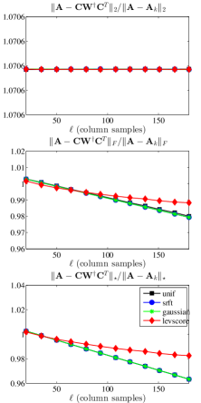
(a) GR, $k=20$

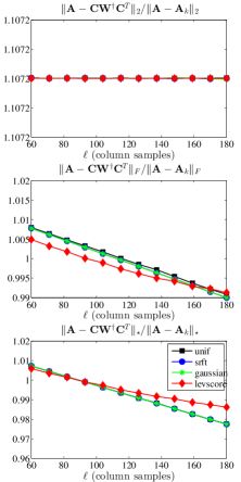
(b) GR, $k=60$

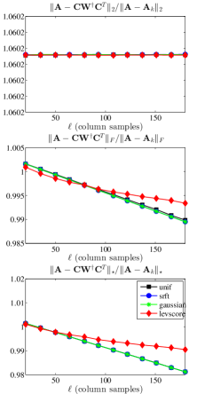
(c) HEP, $k=20$

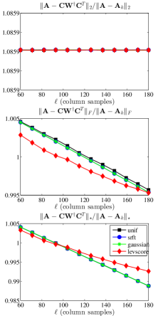
(d) HEP, $k=60$

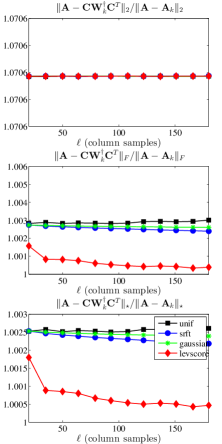
(e) GR, $k=20$

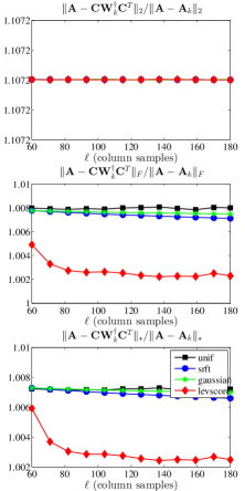
(f) GR, $k=60$

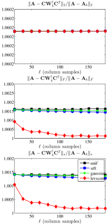
(g) HEP, $k=20$

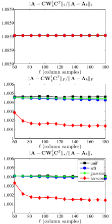
(h) HEP, $k=60$

Figure 1. The spectral, Frobenius, and trace norm errors (top to bottom, respectively, in each subfigure) of several (non-rank-restricted in top panels and rank-restricted in bottom panels) SPSD sketches, as a function of the number of columns samples $\ell$, for the GR and HEP Laplacian data sets, with two choices of the rank parameter $k$.

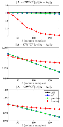
(a) Enron, $k=20$

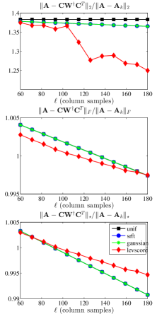
(b) Enron, $k=60$

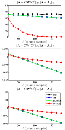
(c) Gnutella, $k=20$

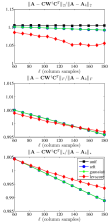
(d) Gnutella, $k=60$

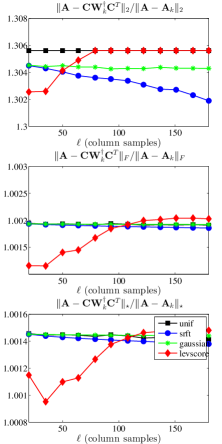
(e) Enron, $k=20$

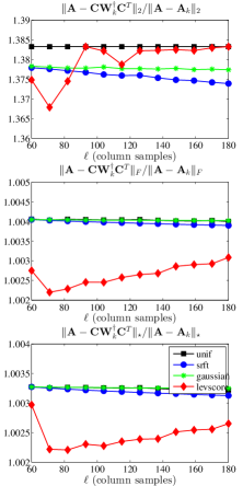
(f) Enron, $k=60$

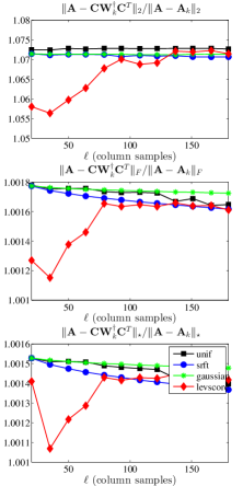
(g) Gnutella, $k=20$

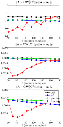
(h) Gnutella, $k=60$

Figure 2. The spectral, Frobenius, and trace norm errors (top to bottom, respectively, in each subfigure) of several (non-rank-restricted in top panels and rank-restricted in bottom panels) SPSD sketches, as a function of the number of columns samples $\ell$, for the Enron and Gnutella Laplacian data sets, with two choices of the rank parameter $k$.

Figure 1 and Figure 2 show the reconstruction error results for sampling and projection methods applied to several normalized graph Laplacians. The former shows GR and HEP, each for two values of the rank parameter, and the latter shows Enron and Gnutella, again each for two values of the rank parameter. Both figures show the spectral, Frobenius, and trace norm approximation errors, as a function of the number of column samples $\ell$, relative to the error of the optimal rank-$k$ approximation of $\mathbf{A}$. In both figures, the first four (i.e., top) subfigures show the results for the non-rank-restricted case, and the last four (i.e., bottom) subfigures show the results for the rank-restricted case. In particular, in the rank-restricted case, the low-rank approximation is “filtered” through a rank-$k$ space, and thus the approximation ratio is always greater than unity.

These and subsequent figures contain a lot of information, some of which is peculiar to the given data sets and some of which is more general. In light of subsequent discussion, several observations are worth making about the results presented in these two figures.

• All of the SPSD sketches provide quite accurate approximations—relative to the best possible approximation factor for that norm, and relative to bounds provided by existing theory, as reviewed in Section 2.4—even with only $k$ column samples (or in the case of the Gaussian and SRFT mixtures, with only $k$ linear combinations of vectors). Upon examination, this is partly due to the extreme sparsity and extremely slow spectral decay of these data sets which means, as shown in Table 4, that only a small fraction of the (spectral or Frobenius or trace) mass is captured by the optimal rank $20$ or $60$ approximation. Thus, although an SPSD sketch constructed from $20$ or $60$ vectors also only captures a small portion of the mass of the matrix, the relative error is small, since the scale of the residual error is large.

• The scale of the Y axes is different between different figures and subfigures. This is to highlight properties within a given plot, but it can hide several things. In particular, note that the scale for the spectral norm is generally larger than for the Frobenius norm, which is generally larger than for the trace norm, consistent with the size of those norms; and that the scale is larger for higher-rank approximations, e.g. compare GR $k=20$ with GR $k=60$, also consistent with the larger amount of mass captured by higher-rank approximations.

• Both the non-rank-restricted and rank-restricted results are the same for $\ell=k$. For $\ell>k$, the non-rank-restricted errors tend to decrease (or at least not increase, as for GR and HEP the spectral norm error is flat as a function of $\ell$), which is intuitive. While the rank-restricted errors also tend to decrease for $\ell>k$, the decrease is much less (since the rank-restricted plots are bounded below by unity) and the behavior is much more complicated as a function of increasing $\ell$.

• The X axes ranges from $k$ to $9k$ for the $k=20$ plots and from $k$ to $3k$ for the $k=60$ plots. As a practical matter, choosing $\ell$ between $k$ and (say) $2k$ or $3k$ is probably of greatest interest. In this regime, there is an interesting tradeoff for the non-rank-restricted plots: for moderately large values of $\ell$ in this regime, the error for leverage-based sampling is moderately better than for uniform sampling or random projections, while if one chooses $\ell$ to be much larger then the improvements from leverage-based sampling saturate and the uniform sampling and random projection methods are better. This is most obvious in the Frobenius norm plots, although it is also seen in the trace norm plots, and it suggests that some combination of leverage-based sampling and uniform sampling might be best.

• For the rank-restricted plots, in some cases, e.g., with GR and HEP, the errors for leverage-based sampling are much better than for the other methods and quickly improve with increasing $\ell$ until they saturate; while in other cases, e.g., with Enron and Gnutella, the errors for leverage-based sampling improve quickly and then degrade with increasing $\ell$. Upon examination, the former phenomenon is similar to what was observed in the non-rank-restricted case and is due to the strong “bias” provided by the leverage score importance sampling distribution to the top part of the spectrum, allowing the sampling process to focus very quickly on the low-rank part of the input matrix. (In some cases, this is due to the fact that the heterogeneity of the leverage score importance sampling distribution means that one is likely to choose the same high leverage columns multiple times, rather than increasing the accuracy of the sketch by adding new columns whose leverage scores are lower.) The latter phenomenon of degrading error quality as $\ell$ is increased is more complex and seems to be due to some sort of “overfitting” caused by this strong bias and by choosing many more than $k$ columns.

• The behavior of the approximations with respect to the spectral norm is quite different from the behavior in the Frobenius and trace norms. In the latter, as the number of samples $\ell$ increases, the errors tend to decrease, although in an erratic manner for some of the rank-restricted plots; while for the former, the errors tend to be much flatter as a function of increasing $\ell$ for at least the Gaussian, SRFT, and uniformly sampled sketches.

All in all, there seems to be quite complicated behavior for low-rank sketches for these Laplacian data sets. Several of these observations can also be made for subsequent figures; but in some other cases the (very sparse and not very low rank) structural properties of the data are primarily responsible.

3.4.2. Linear Kernels

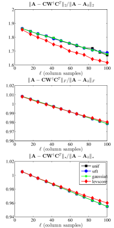
(a) Dexter, $k=8$

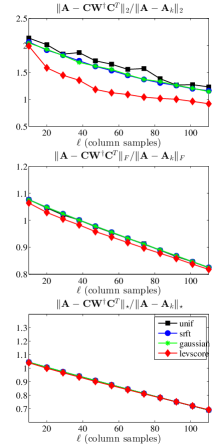
(b) Protein, $k=10$

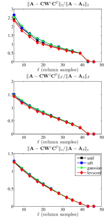
(c) SNPs, $k=5$

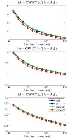
(d) Gisette, $k=12$

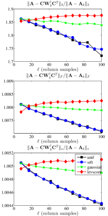
(e) Dexter, $k=8$

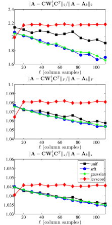
(f) Protein, $k=10$

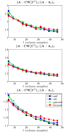
(g) SNPs, $k=5$

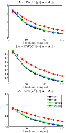
(h) Gisette, $k=12$

Figure 3. The spectral, Frobenius, and trace norm errors (top to bottom, respectively, in each subfigure) of several (non-rank-restricted in top panels and rank-restricted in bottom panels) SPSD sketches, as a function of the number of columns samples $\ell$, for the Linear Kernel data sets.

Figure 3 shows the reconstruction error results for sampling and projection methods applied to several Linear Kernels. The data sets (Dexter, Protein, SNPs, and Gisette) are all quite low-rank and have fairly uniform leverage scores. Several observations are worth making about the results presented in this figure.

• All of the methods perform quite similarly for the non-rank-restricted case: all have errors that decrease smoothly with increasing $\ell$, and in this case there is little advantage to using methods other than uniform sampling (since they perform similarly and are more expensive). Also, since the ranks are so low and the leverage scores are so uniform, the leverage score sketch is no longer significantly distinguished by its tendency to saturate quickly.

• The scale of the Y axes is much larger than for the Laplacian data sets, mostly since the matrices are much more well-approximated by low-rank matrices, although the scale decreases as one goes from spectral to Frobenius to trace reconstruction error, as before.

• For SNPs and Gisette, the rank-restricted reconstruction results are very similar for all four methods, with a smooth decrease in error as $\ell$ is increased, although interestingly using leverage scores is slightly worse for Gisette. For Dexter and Protein, the situation is more complicated: using the SRFT always leads to smooth decrease as $\ell$ is increased, and uniform sampling generally behaves the same way also; Gaussian projections behave this way for Protein, but for Dexter Gaussian projections are noticably worse than SRFT and uniform sampling; and, except for very small values of $\ell$, leverage-based sampling is worse still and gets noticably worse as $\ell$ is increased. Even this poor behavior of leverage score sampling on the Linear Kernels is notably worse than for the rank-restricted Laplacians, where there was a range of moderately small $\ell$ where leverage score sampling was much superior to other methods.

These linear kernels (and also to some extent the dense RBF kernels below that have larger $\sigma$ parameter) are examples of relatively “nice” machine learning data sets that are similar to matrices where uniform sampling has been shown to perform well previously [58, 37, 38, 39]; and for these matrices our empirical results agree with these prior works.

3.4.3. Dense and Sparse RBF Kernels

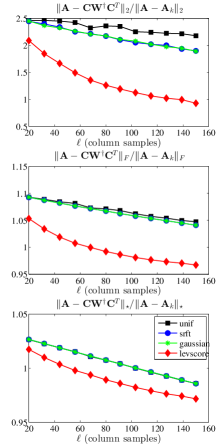
(a) AbaloneD, $\sigma=.15,k=20$

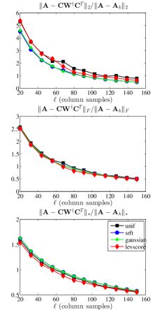
(b) AbaloneD, $\sigma=1,k=20$

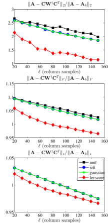
(c) WineD, $\sigma=1,k=20$

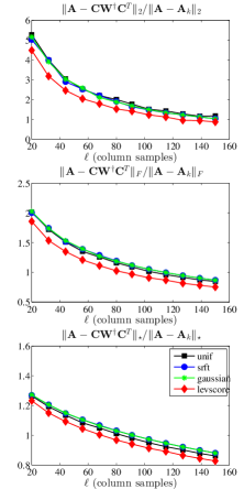
(d) WineD, $\sigma=2.1,k=20$

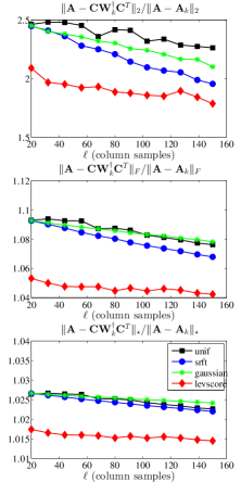
(e) AbaloneD, $\sigma=.15,k=20$

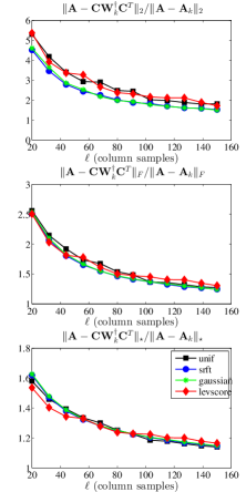
(f) AbaloneD, $\sigma=1,k=20$

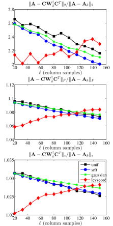
(g) WineD, $\sigma=1,k=20$

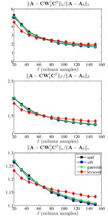
(h) WineD, $\sigma=2.1,k=20$

Figure 4. The spectral, Frobenius, and trace norm errors (top to bottom, respectively, in each subfigure) of several (non-rank-restricted in top panels and rank-restricted in bottom panels) SPSD sketches, as a function of the number of columns samples $\ell$, for several dense RBF data sets.

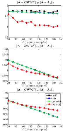
(a) AbaloneS, $\sigma=.15,k=20$

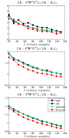
(b) AbaloneS, $\sigma=1,k=20$

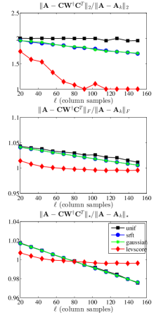
(c) WineS, $\sigma=1,k=20$

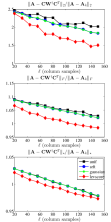
(d) WineS, $\sigma=2.1,k=20$

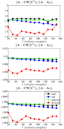
(e) AbaloneS, $\sigma=.15,k=20$

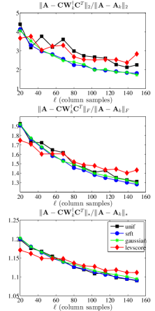
(f) AbaloneS, $\sigma=1,k=20$

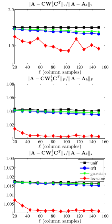
(g) WineS, $\sigma=1,k=20$

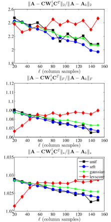
(h) WineS, $\sigma=2.1,k=20$

Figure 5. The spectral, Frobenius, and trace norm errors (top to bottom, respectively, in each subfigure) of several (non-rank-restricted in top panels and rank-restricted in bottom panels) SPSD sketches, as a function of the number of columns samples $\ell$, for several sparse RBF data sets.

Figure 4 and Figure 5 present the reconstruction error results for sampling and projection methods applied to several dense RBF and sparse RBF kernels. Several observations are worth making about the results presented in these figures.

• For the non-rank-restricted results, all of the methods have errors that decrease with increasing $\ell$. In particular, for larger values of $\sigma$ and for denser data, the decrease is somewhat more regular, and the four methods tend to perform similarly. For larger values of $\sigma$ and sparser data, leverage score sampling is somewhat better. This parallels what we observed with the Linear Kernels, except that here the leverage score sampling is somewhat better for all values of $\ell$.

• For the non-rank-restricted results for the smaller values of $\sigma$, leverage score sampling tends to be much better than uniform sampling and projection-based methods. For the sparse data, however, this effect saturates; and we again observe (especially when $\sigma$ is smaller in AbaloneS and WineS) the tradeoff we observed previously with the Laplacian data—leverage score sampling is better when $\ell$ is moderately larger than $k$, while uniform sampling and random projections are better when $\ell$ is much larger than $k$.

• For the rank-restricted results, we see that when $\sigma$ is large, all of the results tend to perform similarly. (The exception to this is WineS, for which leverage score sampling starts out much better than other methods and then gets worse as $\ell$ is increased.) On the other hand, when $\sigma$ is small, the results are more complex. Leverage score sampling is typically much better than other methods, although the results are quite choppy as a function of $\ell$, and in some cases the effect diminished as $\ell$ is increased.

Recall from Table 5 that for smaller values of $\sigma$ and for sparser kernels, the SPSD matrices are less well-approximated by low-rank matrices, and they have more heterogeneous leverage scores. Thus, they are more similar to the Laplacian data than the Linear Kernel data; and this suggests (as we have observed) that leverage score sampling should perform relatively better than uniform column sampling and projection-based schemes when in these two cases. In particular, nowhere do we see that leverage score sampling performs much worse than other methods, as we saw with the rank-restricted Linear Kernel results.

3.4.4. Summary of Comparison of Sampling and Projection Algorithms

Before proceeding, there are several summary observations that we can make about sampling versus projection methods for the data sets we have considered.

• Linear Kernels and to a lesser extent Dense RBF Kernels with larger $\sigma$ parameter have relatively low-rank and relatively uniform leverage scores, and in these cases uniform sampling does quite well. These data sets correspond most closely with those that have been studied previously in the machine learning literature, and for these data sets our results are in agreement with that prior work.

• Sparsifying RBF Kernels and/or choosing a smaller $\sigma$ parameter tends to make these kernels less well-approximated by low-rank matrices and to have more heterogeneous leverage scores. In general, these two properties need not be directly related—the spectrum is a property of eigenvalues, while the leverage scores are determined by the eigenvectors—but for the data we examined they are related, in that matrices with more slowly decaying spectra also often have more heterogeneous leverage scores.

• For Dense RBF Kernels with smaller $\sigma$ and Sparse RBF Kernels, leverage score sampling tends to do much better than other methods. Interestingly, the Sparse RBF Kernels have many properties of very sparse Laplacian Kernels corresponding to relatively-unstructured informatics graphs, an observation which should be of interest for researchers who construct sparse graphs from data using, e.g., “locally linear” methods, to try to reconstruct hypothesized low-dimensional manifolds.

• Reconstruction quality under leverage score sampling saturates, as a function of choosing more samples $\ell$; this is seen both for non-rank-restricted and rank-restricted situations. As a consequence, there can be a tradeoff between leverage score sampling or other methods being better, depending on the values of $\ell$ that are chosen.

• Although they are potentially ill-conditioned, non-rank-restricted approximations behave better in terms of reconstruction quality. Rank-constrained approximations tend to have much more complicated behavior as a function of increasing the numbe of samples $\ell$, including choppier and non-monotonic behavior. This is particularly severe for leverage score sampling, but it occurs with other methods; and it suggests that other forms of regularization (other than what is essentially a Tikhonov form of regularization for the rank-restricted cases) might be appropriate.

In general, all of the sampling and projection methods we considered perform much better on the SPSD matrices we considered than previous worst-case bounds (e.g., [21, 39, 28]) would suggest. (That is, even the worst results correspond to single-digit approximation factors in relative scale.) This observation is intriguing, because the motivation of leverage score sampling (and, recall, that in this context random projections should be viewed as performing uniform random sampling in a randomly-rotated basis where the leverage scores have been approximately uniformized [46]) is very much tied to the Frobenius norm, and so there is no a priori reason to expect its good performance to extend to the spectral or trace norms. Motivated by this, we revisit the question of proving improved worst-case theoretical bounds in Section 4.

Before describing these improved theoretical results, however, we address in Section 3.5 running time questions. After all, a naïve implementation of sampling with exact leverage scores is slower than other methods (and much slower than uniform sampling). As shown below, by using the recently-developed approximation algorithm of [20], not only does this approximation algorithm run in time comparable with random projections (for certain parameter settings), but it leads to approximations that soften the strong bias that the exact leverage scores provide toward the best rank-$k$ approximation to the matrix, thereby leading to improved reconstruction results in many cases.

3.5. Reconstruction Accuracy of Leverage Score Approximation Algorithms

A naïve view might assume that computing probabilities that permit leverage-based sampling requires an $O(n^{3})$ computation of the full SVD, or at least the full computation of a partial SVD, and thus that it would be much more expensive than recently-developed random projection methods. Indeed, an “exact” computation of the leverage scores with a QR decomposition or truncated SVD takes roughly $\mathrm{O}(n^{2}k)$ time (and the running time results of Section 3.4 actually used this naïve procedure). Recent work, however, has shown that relative-error approximations to all the statistical leverage scores can be computed more quickly than this exact algorithm [20]. Here, we implement and evaluate a version of this algorithm, and we evaluate it both in terms of running time and in terms of reconstruction quality on the diverse suite of real data matrices we considered above. We note that ours is the first work to provide an empirical evaluation of an implementation of the leverage score approximation algorithms of [20], illustrating empirically the tradeoffs between cost and efficiency in a practical setting.

3.5.1. Description of the Fast Approximation Algorithm of [20]

Input: $\mathbf{A}\in\mathbb{R}^{n\times d}$ (with SVD $\mathbf{A}=\mathbf{U}\boldsymbol{\Sigma}\mathbf{V}^{T}$), error parameter $\epsilon\in(0,1/2]$.

Output: $\tilde{\ell_{i}},i=1,\ldots,n$, approximations to the leverage scores of $\mathbf{A}.$

1. Let $\boldsymbol{\Pi}_{1}\in\mathbb{R}^{r_{1}\times n}$ be an SRFT with

   $$r_{1}=\Omega(\epsilon^{-2}(\sqrt{d}+\sqrt{\ln n})^{2}\ln d)$$

2. Compute $\boldsymbol{\Pi}_{1}\mathbf{A}\in\mathbb{R}^{r_{1}\times d}$ and its QR factorization $\boldsymbol{\Pi}_{1}\mathbf{A}=\mathbf{Q}\mathbf{R}$.

3. Let $\boldsymbol{\Pi}_{2}\in\mathbb{R}^{d\times r_{2}}$ be a matrix of i.i.d. standard Gaussian random variables, where

   $$r_{2}=\Omega\left(\epsilon^{-2}\ln n\right).$$

4. Construct the product $\boldsymbol{\Omega}=\mathbf{A}\mathbf{R}^{-1}\boldsymbol{\Pi}_{2}.$

5. For $i=1,\ldots,n$ compute $\tilde{\ell}_{i}=\left\|\Omega_{(i)}\right\|_{2}^{2}$.

Algorithm 1 Algorithm (originally Algorithm 1 in [20]) for approximating the leverage scores $\ell_{i}$ of an $n\times d$ matrix $\mathbf{A}$, where $n\gg d$, to within a multiplicative factor of $1\pm\epsilon$. The running time of the algorithm is $\mathrm{O}(nd\ln(\sqrt{d}+\sqrt{\ln n})+nd\epsilon^{-2}\ln n+d^{2}\epsilon^{-2}(\sqrt{d}+\sqrt{\ln n})^{2}\ln d).$

Input: $\mathbf{A}\in\mathbb{R}^{n\times d},$ a rank parameter $k,$ and an error parameter $\epsilon\in(0,1/2].$

Output: $\hat{\ell_{i}},i=1,\ldots,n$, approximations to the leverage scores of $\mathbf{A}$ filtered through its dominant dimension-$k$ subspace.

1. Construct $\boldsymbol{\Pi}\in\mathbb{R}^{d\times 2k}$ with i.i.d. standard Gaussian entries.

2. Compute $\mathbf{B}=\left(\mathbf{A}\mathbf{A}^{T}\right)^{q}\mathbf{A}\boldsymbol{\Pi}\in\mathbb{R}^{n\times 2k}$ with

   $$q\geq\left\lceil\frac{\ln\left(1+\sqrt{\frac{k}{k-1}}+\mathrm{e}\sqrt{\frac{2}{k}}\sqrt{\min\left\{n,d\right\}-k}\right)}{2\ln\left(1+\epsilon/10\right)-1/2}\right\rceil,$$

3. Approximate the leverage scores of $\mathbf{B}$ by calling Algorithm 1 with inputs $\mathbf{B}$ and $\epsilon$; let $\hat{\ell}_{i}$ for $i=1,\ldots,n$ be the outputs of Algorithm 1.

Algorithm 2 Algorithm (originally Algorithm 4 in [20]) for approximating the leverage scores (relative to the best rank-$k$ approximation to $\mathbf{A}$) of a general $n\times d$ matrix $\mathbf{A}$ with those of a matrix that is close by in the spectral norm (or the Frobenius norm if $q=0$). This algorithm runs in time $\mathrm{O}(ndkq)+T_{1}$, where $T_{1}$ is the running time of Algorithm 1.

Input: $\mathbf{A}\in\mathbb{R}^{n\times d}$, a rank parameter $k$, and an iteration parameter $q$.

Output: $\hat{\ell_{i}},i\in=1,\ldots,n,$ approximations to the leverage scores of $\mathbf{A}$ filtered through its dominant dimension-$k$ subspace.

1. Construct an SRHT matrix $\boldsymbol{\Pi}\in\mathbb{R}^{d\times r},$ where

   $$r\geq\left\lceil 36\epsilon^{-2}[\sqrt{k}+\sqrt{8\ln(kd)}]^{2}\ln(k)\right\rceil.$$

2. Compute $\mathbf{B}=\left(\mathbf{A}\mathbf{A}^{T}\right)^{q}\mathbf{A}\boldsymbol{\Pi}\in\mathbb{R}^{n\times r},$ where $q\geq 0$ is an integer.

3. Return the exact leverage scores of $\mathbf{B}.$

Algorithm 3 Algorithm for approximating the leverage scores (relative to the best rank-$k$ approximation to $\mathbf{A}$) of a general $n\times d$ matrix $\mathbf{A}$ with those of a matrix that is close by in the spectral norm. This is a modified version of Algorithm 2, in which the random projection is implemented with an SRFT rather than a Gaussian random matrix, and where the number of “iterations” $q$ is prespecified. This algorithm runs in time $\mathrm{O}(nd\ln r+ndrq+nr^{2})$ since $\mathbf{A}\boldsymbol{\Pi}$ can be computed in time $\mathrm{O}(nd\ln r).$

Algorithm 1 (which originally appeared as Algorithm 1 in [20]) takes as input an arbitrary $n\times d$ matrix $\mathbf{A}$, where $n\gg d$, and it returns as output a $1\pm\epsilon$ approximation to all of the statistical leverage scores of the input matrix. The original algorithm of [20] uses a subsampled Hadamard transform and requires $r_{1}$ to be somewhat larger than what we state in Algorithm 1. That an SRFT with a smaller value of $r_{1}$ can be used instead is a consequence of the fact that Lemma 3 in [20] is also satisfied by an SRFT matrix with the given $r_{1};$ this is established in [60, 13].

The running time of this algorithm, given in the caption of the algorithm, is roughly $O(nd\ln d)$ when $d=\Omega(\ln n)$. Thus Algorithm 1 generates relative-error approximations to the leverage scores of a tall and skinny matrix $\mathbf{A}$ in time $o(nd^{2})$, rather than the $\mathrm{O}(nd^{2})$ time that would be required to compute a QR decomposition or a thin SVD of the $n\times d$ matrix $\mathbf{A}$. The basic idea behind Algorithm 1 is as follows. If we had a QR decomposition of $\mathbf{A}$, then we could postmultiply $\mathbf{A}$ by the inverse of the “$R$” matrix to obtain an orthogonal matrix spanning the column space of $\mathbf{A}$; and from this $n\times d$ orthogonal matrix, we could read off the leverage scores from the Euclidean norms of the rows. Of course, computing the QR decomposition would require $O(nd^{2})$ time. To get around this, Algorithm 1 premultiplies $\mathbf{A}$ by a structured random projection $\boldsymbol{\Pi}_{1}$, computes a QR decomposition of $\boldsymbol{\Pi}_{1}\mathbf{A}$, and postmultiplies $\mathbf{A}$ by $\mathbf{R}^{-1}$, i.e., the inverse of the “$R$” matrix from the QR decomposition of $\boldsymbol{\Pi}_{1}\mathbf{A}$. Since $\boldsymbol{\Pi}_{1}$ is an SRFT, premultiplying by it takes roughly $O(nd\ln d)$ time. In addition, note that $\boldsymbol{\Pi}_{1}\mathbf{A}$ needs to be post multiplied by a second random projection in order to compute all of the leverage scores in the allotted time; see [20] for details. This algorithm is simpler than the algorithm in which we are primarily interested that is applicable to square SPSD matrices, but we start with it since it illustrates the basic ideas of how our main algorithm works and since our main algorithm calls it as a subroutine. We note, however, that this algorithm is directly useful for approximating the leverage scores of Linear Kernel matrices $\mathbf{A}=\mathbf{X}\mathbf{X}^{T}$, when $\mathbf{X}$ is a tall and skinny matrix.

Consider, next, Algorithm 2 (which originally appeared as Algorithm 4 in [20]), which takes as input an arbitrary $n\times d$ matrix $\mathbf{A}$ and a rank parameter $k$, and returns as output a $1\pm\epsilon$ approximation to all of the statistical leverage scores (relative to the best rank-$k$ approximation) of the input. An important technical point is that the problem of computing the leverage scores of a matrix relative to a low-dimensional space is ill-posed, essentially because the spectral gap between the $k^{th}$ and the $(k+1)^{st}$ eigenvalues can be small, and thus Algorithm 2 actually computes approximations to the leverage scores of a matrix that is near to $\mathbf{A}$ in the spectral norm (or the Frobenius norm if $q=0$). See [20] for details. Basically, this algorithm uses Gaussian sampling to find a matrix close to $\mathbf{A}$ in the Frobenius norm or spectral norm, and then it approximates the leverage scores of this matrix by using Algorithm 1 on the smaller, very rectangular matrix $\mathbf{B}$. When $\mathbf{A}$ is square, as in our applications, Algorithm 2 is typically more costly than direct computation of the leverage scores, at least for dense matrices (but it does have the advantage that the number of iterations is bounded, independent of properties of the matrix, which is not true for typical iterative methods to compute low-rank approximations).

Of greater practical interest is Algorithm 3, which is a modification of Algorithm 2 in which the Gaussian random projection is replaced with an SRFT. That is, Algorithm 3 uses an SRFT projection to find a matrix close by to $\mathbf{A}$ in the Frobenius norm or spectral norm (depending on the value of $q$), and then it exactly computes the leverage scores of this matrix. This improves the running time to $\mathrm{O}(n^{2}\ln(\sqrt{k}+\sqrt{\ln n})+n^{2}(\sqrt{k}+\sqrt{\ln n})^{2}\ln(k)q+n(\sqrt{k}+\sqrt{\ln n})^{4}\ln^{2}(k)),$ which is $o(n^{2}k)$ when $q=0$. Thus an important point for Algorithm 3 (as well as for Algorithm 2) is the parameter $q$ which describes the number of iterations. For $q=0$ iterations, we get an inexpensive Frobenius norm approximation; while for higher $q$, we get better spectral norm approximations that are more expensive This flexibility is of interest, as one may want to approximate the actual leverage scores accurately or one may simply want to find crude approximations useful for obtaining SPSD sketches with low reconstruction error.

Finally, note that although choosing the number of iterations $q$ as we did in Algorithm 2 is convenient for worst-case analysis, as a practical implementational matter it is easier either to choose $q$ based on spectral gap information revealed during the running of the algorithm or to prespecify $q$ to be a small integer, e.g., $2$ or $3$, before the algorithm runs. Both of these have an interpretation of accelerating the rate of decay of the spectrum with a power iteration, but they behave somewhat differently due to the different stopping conditions. Below, we consider both variants.

3.5.2. Running Time Comparisons

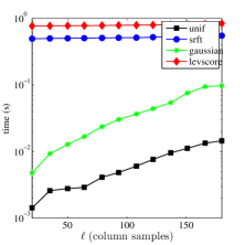
(a) GR, $k=20$

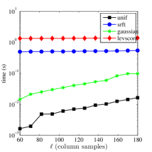
(b) GR, $k=60$

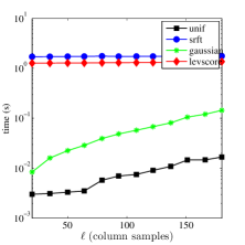
(c) HEP, $k=20$

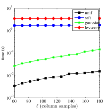
(d) HEP, $k=60$

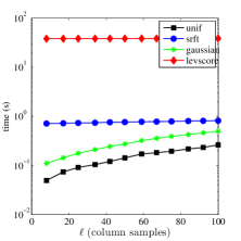
(e) Dexter, $k=8$

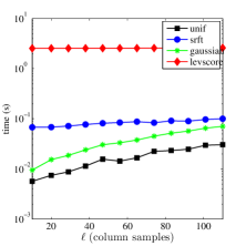
(f) Protein, $k=10$

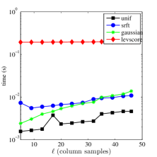
(g) SNPs, $k=5$

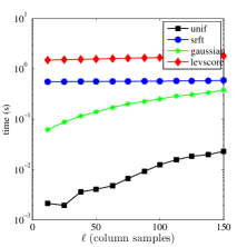
(h) Gisette, $k=12$

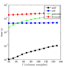
(i) AbaloneD, $\sigma=.15,k=20$

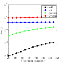
(j) AbaloneD, $\sigma=1,k=20$

(k) WineD, $\sigma=1,k=20$

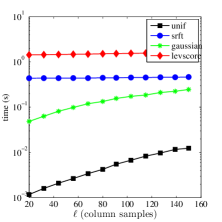
(l) WineD, $\sigma=2.1,k=20$

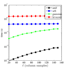
(m) AbaloneS, $\sigma=.15,k=20$

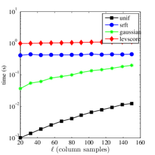
(n) AbaloneS, $\sigma=1,k=20$

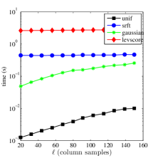
(o) WineS, $\sigma=1,k=20$

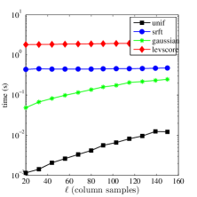
(p) WineS, $\sigma=2.1,k=20$

Figure 6. The times required to compute the (non-rank-restricted) SPSD sketches, as a function of the number of columns samples $\ell$ for several data sets and two choices of the rank parameter $k$.

(a) GR, $k=20$

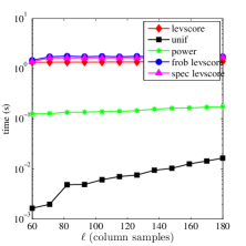
(b) GR, $k=60$

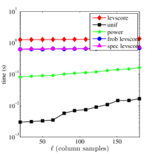
(c) HEP, $k=20$

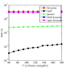
(d) HEP, $k=60$

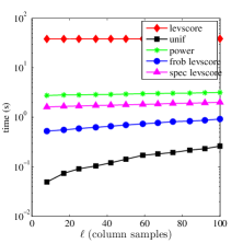
(e) Dexter, $k=8$

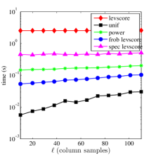
(f) Protein, $k=10$

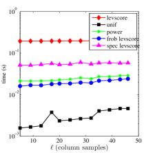
(g) SNPs, $k=5$

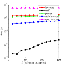
(h) Gisette, $k=12$

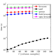
(i) AbaloneD, $\sigma=.15,k=20$

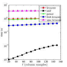
(j) AbaloneD, $\sigma=1,k=20$

(k) WineD, $\sigma=1,k=20$

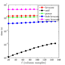
(l) WineD, $\sigma=2.1,k=20$

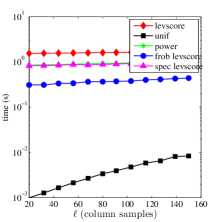
(m) AbaloneS, $\sigma=.15,k=20$

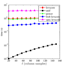
(n) AbaloneS, $\sigma=1,k=20$

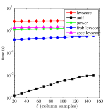
(o) WineS, $\sigma=1,k=20$

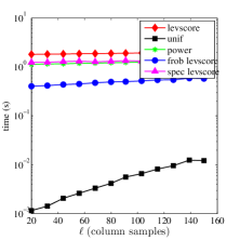
(p) WineS, $\sigma=2.1,k=20$

Figure 7. The times required to compute the (non-rank-restricted) approximate leverage score-based SPSD sketches, as a function of the number of columns samples $\ell$ for several data sets.

(a) Protein, $k=10$

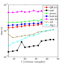
(b) SNPs, $k=5$

Figure 8. The running time of (non-rank-restricted) SPSD sketches computed using Algorithm 1 compared with that of other approximate leverage score-based SPSD sketches, as a function of the number of column samples $\ell$ for two Linear Kernel datasets. The parameters in Algorithm 1 were taken to be $r_{1}=\epsilon^{-2}\ln(d\delta^{-1})(\sqrt{d}+\sqrt{\ln(n\delta^{-1})})^{2}$ and $r_{2}=\epsilon^{-2}(\ln n+\ln\delta^{-1})$ with $\epsilon=1$ and $\delta=1/10.$

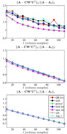
(a) Protein, $k=10$, non-rank-restricted

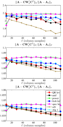
(b) Protein, $k=10$, rank-restricted

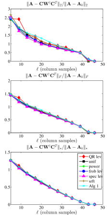
(c) SNPs, $k=5$, non-rank-restricted

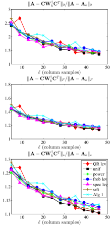
(d) SNPs, $k=5$, rank-restricted

Figure 9. The spectral, Frobenius, and trace norm errors (top to bottom, respectively, in each subfigure) of SPSD sketches computed using Algorithm 1 compared with those of other approximate leverage score-based sketching schemes, as a function of the number of columns samples $\ell$, for two Linear Kernel data sets. The parameters in Algorithm 1 were taken to be $r_{1}=\epsilon^{-2}\ln(d\delta^{-1})(\sqrt{d}+\sqrt{\ln(n\delta^{-1})})^{2}$ and $r_{2}=\epsilon^{-2}(\ln n+\ln\delta^{-1})$ with $\epsilon=1$ and $\delta=1/10.$

Here, we describe the performances of the various random sampling and random projection low-rank sketches considered in Section 3.4 in terms of their running time, where the method that involves using the leverage scores to construct the importance sampling distribution is implemented both by computing the leverage scores “exactly” by calling a truncated SVD, as a black box, as well as computing them approximately by using one of several versions of Algorithm 3. Our running time results are presented in Figure 6 and Figure 7.

We start with the results described in Figure 6, which shows the running times, as a function of $\ell$, for the low-rank approximations described in Section 3.4: i.e., for column sampling uniformly at random without replacement; for column sampling according to the exact nonuniform leverage score probabilities; and for sketching using Gaussian and SRFT mixtures of the columns. Several observations are worth making about the results presented in this figure.

• Uniform sampling is always less expensive and typically much less expensive than the other methods, while (with one minor exception) sampling according to the exact leverage scores is always the most expensive method.

• For most matrices, using the SRFT is nearly as expensive as exact leverage score sampling. This is most true for the very sparse graph Laplacian Kernels, largely since the SRFT does not respect sparsity. The main exception to this is for the dense and relatively well-behaved Linear Kernels, where especially for large values of $\ell$ the SRFT is quite fast and usually not too much more expensive than uniform sampling.

• The “fast Fourier” methods underlying the SRFT can take advantage of the structure of the Linear Kernels to yield algorithms that are similar to Gaussian projections and much better than exact leverage score computation. Note that the reason that SRFT is worse than Gaussians here is that the matrices we are considering are not extremely large, and we are not considering very large values of the rank parameter. Extending in both those directions leads to Gaussian projections being slower than SRFT, as the trends in the figures clearly indicate.

• Gaussian projections are not too much slower than uniform sampling for the extremely sparse Laplacian Kernels—this is due to the sparsity of the Laplacian Kernels, since Gaussian projections can take advantage of the fast matrix-vector multiply, while the SRFT-based scheme cannot—but this advantage is lost for the (denser) Sparse RBF Kernels, to the extent that there is little running time improvement relative to the Dense RBF Kernels. In addition, Gaussian projections are relatively slower, when compared to the SRFT and uniform sampling, for the Dense RBF Kernels than for the Linear Kernels, although both of those data sets are maximally dense.

We next turn to the results described in Figure 7, which shows the running times, as a function of $\ell$, for several variants of approximate leverage-based sampling. For ease of comparison, the timings for uniform sampling (“unif”) and exact leverage score sampling (“levscore”) are depicted in Figure 7 using the same shading as used in Figure 6. In addition to these two baselines, Figure 7 shows running time results for the following three variants of approximate leverage score sampling: “frob levscore” (which is Algorithm 3 with $q=0$ and $r=2k$); “spec levscore” (Algorithm 3 with $q=4$ and $r=2k$); and “power”. The “power” scheme is a version of Algorithm 3 where $r=k$ and $q$ is determined by monitoring the convergence of the leverage scores of $\mathbf{A}^{2q+1}\boldsymbol{\Pi}$ and terminating when the change in the leverage scores between iterations, as measured in the infinity norm, is smaller than $10^{-2}.$ This is simply a version of subspace iteration with a convergence criterion appropriate for the task at hand. Since “frob levscore” requires one application of an SRFT, its timing results are depicted using the same shade as the SRFT timing results in Figure 6. (There are no other correspondences between the shadings in the two figures.) Several observations are worth making about the results presented in this figure.

• These approximate leverage score-based algorithms can be orders of magnitude faster than exact leverage score computation; but, especially for “spec levscore” when $q$ is not prespecified to be $2$ or $3$, they can even be somewhat slower. Exactly which is the case depends upon the properties of the matrix and the parameters used in the approximation algorithm, including especially the number of power iterations.

• The “frob levscore” approximation method has running time comparable to the running time of the SRFT, which is expected, given that the computation of the SRFT is the theoretical bottleneck for the running time of the “frob levscore” algorithm. In particular, for larger values of $\ell$ for Linear Kernels, “frob levscore” is not much slower than uniform sampling.

• The “spec levscore” and “power” approximations with $q>0$ are more expensive than the $q=0$ “frob lev” approximation, which is a result of the relatively-expensive matrix-matrix multiplication. For the Linear Kernels, both are much better than the exact leverage score computation, and for most other data at least “power” is somewhat less expensive than the exact leverage score computation. For example, this is particularly true for the Laplacian Kernels.

Recall that the cost associated with these SPSD sketches is two-fold: first, the cost to construct the sample—by sampling columns uniformly at random, by computing a nonuniform importance sampling distribution, or by performing a random projection to uniformize the leverage scores; and second, the cost to construct the low-rank approximation from the sample. For uniform sampling, the latter step dominates the cost, while for more sophisticated methods the former step typically dominates the cost. The approximate leverage score sampling methods are still sufficiently expensive that the cost of computing the sampling probabilities still dominates the cost to construct the low-rank approximation.

Finally, Algorithm 1 can be used to approximate quickly the leverage scores of matrices of the form $\mathbf{A}=\mathbf{X}\mathbf{X}^{T}$, when $\mathbf{X}\in\mathbb{R}^{n\times d}$ is a rectangular matrix of sufficent aspect ratio, and in such cases it is faster than Algorithm 3. Specifically, for the first dimensional reduction step in Algorithm 1 to be beneficial (i.e., to ensure $r_{1}<n$), the condition $n=\Omega(d\ln d)$ is necessary; for the second dimensional reduction step to be beneficial (i.e., to ensure $r_{2}<d$), the condition $d=\Omega(\ln n)$ must be satisfied. Figure 8 summarizes our main results for the run time of Algorithm 1 applied to rectangular matrices with $n\gg d$. Among other things, Figure 8 illustrates, using the Linear Kernel datasets Protein and SNPs (which satisfy these constraints), two points.

• Most importantly, the running time of Algorithm 1 on these rectangular matrices is faster than performing a QR decomposition on $\mathbf{A}$ and is comparable to applying a SRFT to $\mathbf{A}$. This is expected, since the running time bottleneck for Algorithm 1 is the application of the SRFT.

• In addition, the running time of Algorithm 1 is significantly faster than the other approximate leverage score algorithms. This too is expected, since these other algorithms are applied to $\mathbf{A}$ and ignore the rectangular structure of $\mathbf{X}$.

Figure 9 shows that these improved running time gains for Algorithm 1 can come at the cost of a slight loss in the reconstruction accuracy (relative to the exact computation of the leverage scores) of the low-rank approximations; the accuracy of the other approximate leverage score algorithms is discussed in the following subsection.

3.5.3. Reconstruction Accuracy Results

Here, we describe the performances of the various low-rank approximations that use approximate leverage scores in terms of reconstruction accuracy for the data sets described in Section 3.1. The results are presented in Figure 10 through Figure 14. The setup for these results parallels that for the low-rank approximation results described in Section 3.4, and these figures parallel Figure 1 through Figure 5. To provide a baseline for the comparison, we also plot the previous reconstruction errors for sampling with the exact leverage scores as well as the uniform column sampling sketch. Several observations are worth making about the results presented in these figures.

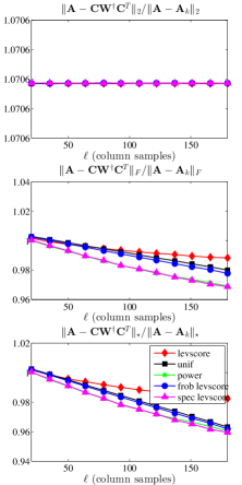
(a) GR, $k=20$

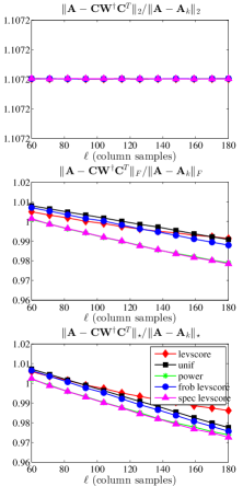
(b) GR, $k=60$

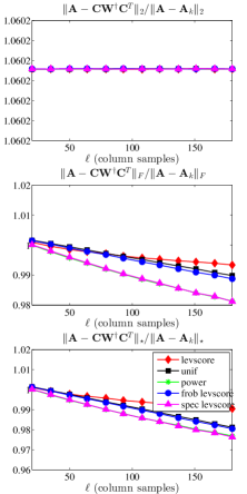
(c) HEP, $k=20$

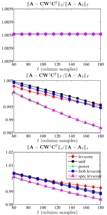
(d) HEP, $k=60$

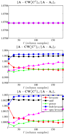
(e) GR, $k=20$

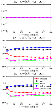
(f) GR, $k=60$

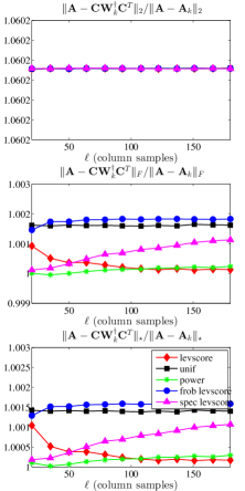
(g) HEP, $k=20$

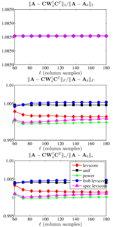
(h) HEP, $k=60$

Figure 10. The spectral, Frobenius, and trace norm errors (top to bottom, respectively, in each subfigure) of several (non-rank-restricted in top panels and rank-restricted in bottom panels) approximate leverage score-based SPSD sketches, as a function of the number of columns samples $\ell$, for the GR and HEP Laplacian data sets, with two choices of the rank parameter $k$.

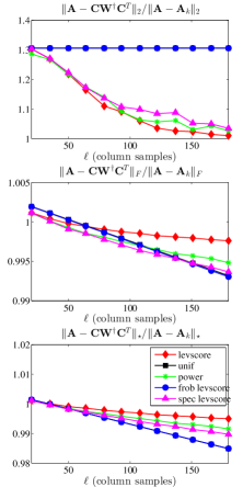
(a) Enron, $k=20$

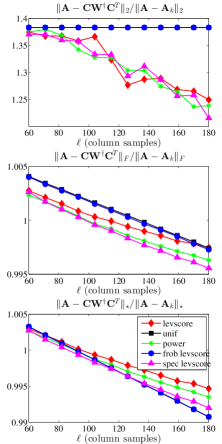
(b) Enron, $k=60$

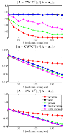
(c) Gnutella, $k=20$

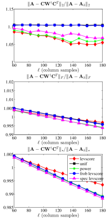
(d) Gnutella, $k=60$

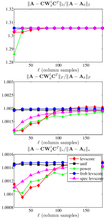
(e) Enron, $k=20$

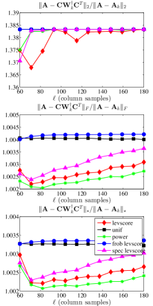
(f) Enron, $k=60$

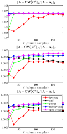
(g) Gnutella, $k=20$

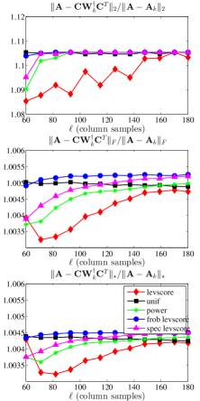
(h) Gnutella, $k=60$

Figure 11. The spectral, Frobenius, and trace norm errors (top to bottom, respectively, in each subfigure) of several (non-rank-restricted in top panels and rank-restricted in bottom panels) approximate leverage score-based SPSD sketches, as a function of the number of columns samples $\ell$, for the Enron and Gnutella Laplacian data sets, with two choices of the rank parameter $k$.

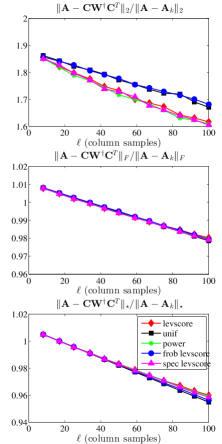
(a) Dexter, $k=8$

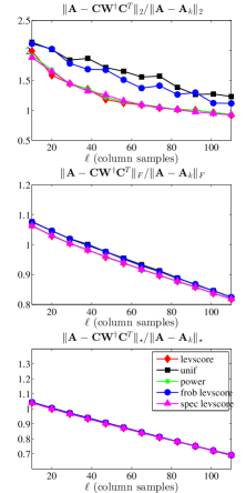
(b) Protein, $k=10$

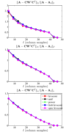
(c) SNPs, $k=5$

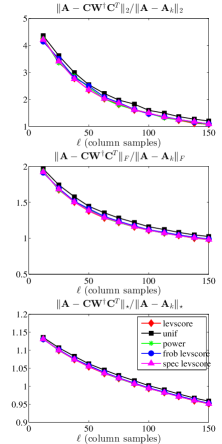
(d) Gisette, $k=12$

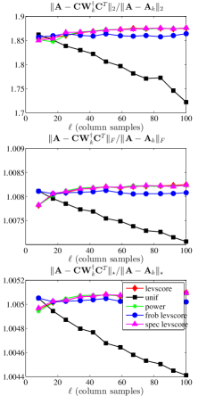
(e) Dexter, $k=8$

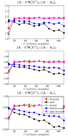
(f) Protein, $k=10$

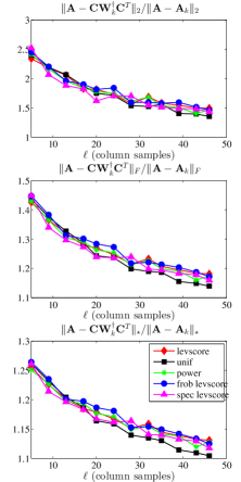
(g) SNPs, $k=5$

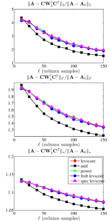
(h) Gisette, $k=12$

Figure 12. The spectral, Frobenius, and trace norm errors (top to bottom, respectively, in each subfigure) of several (non-rank-restricted in top panels and rank-restricted in bottom panels) approximate leverage score-based SPSD sketches, as a function of the number of columns samples $\ell$, for the Linear Kernel data sets

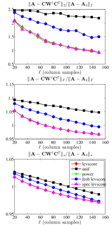
(a) AbaloneD, $\sigma=.15,k=20$

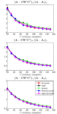
(b) AbaloneD, $\sigma=1,k=20$

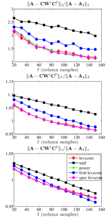
(c) WineD, $\sigma=1,k=20$

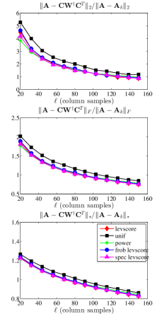
(d) WineD, $\sigma=2.1,k=20$

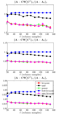
(e) AbaloneD, $\sigma=.15,k=20$

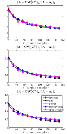
(f) AbaloneD, $\sigma=1,k=20$

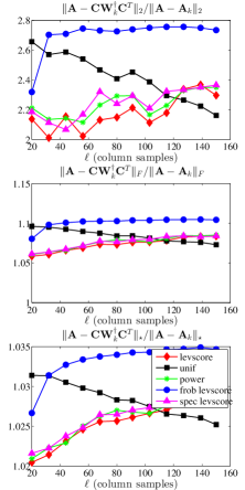
(g) WineD, $\sigma=1,k=20$

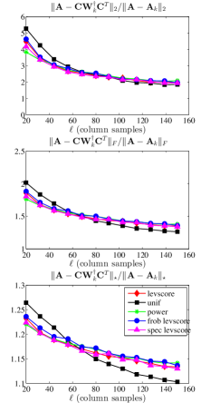
(h) WineD, $\sigma=2.1,k=20$

Figure 13. The spectral, Frobenius, and trace norm errors (top to bottom, respectively, in each subfigure) of several (non-rank-restricted in top panels and rank-restricted in bottom panels) approximate leverage score-based SPSD sketches, as a function of the number of columns samples $\ell$, for several dense RBF data sets.

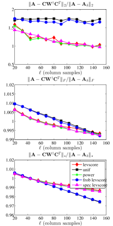
(a) AbaloneS, $\sigma=.15,k=20$

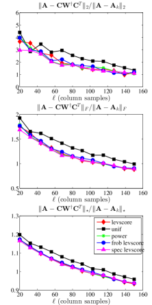
(b) AbaloneS, $\sigma=1,k=20$

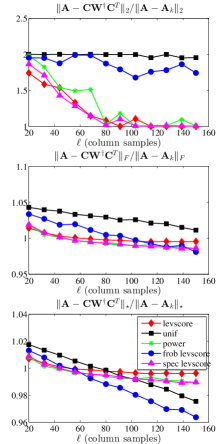
(c) WineS, $\sigma=1,k=20$

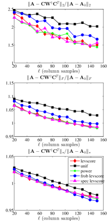
(d) WineS, $\sigma=2.1,k=20$

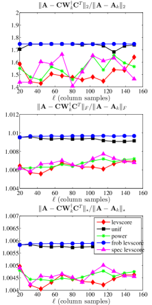
(e) AbaloneS, $\sigma=.15,k=20$

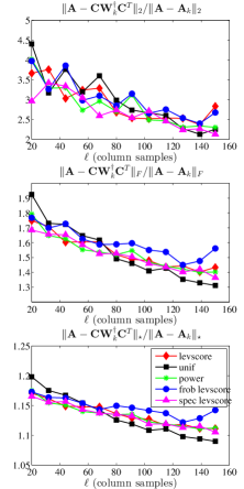
(f) AbaloneS, $\sigma=1,k=20$

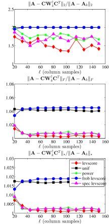
(g) WineS, $\sigma=1,k=20$

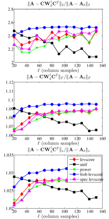
(h) WineS, $\sigma=2.1,k=20$

Figure 14. The spectral, Frobenius, and trace norm errors (top to bottom, respectively, in each subfigure) of several (non-rank-restricted in top panels and rank-restricted in bottom panels) approximate leverage score-based SPSD sketches, as a function of the number of columns samples $\ell$, for several sparse RBF data sets.

• For Laplacian Kernels, for the non-rank-restricted results, “frob levscore” is only slightly better than uniform sampling, while “power” and “spec levscore” are substantially better than uniform sampling. All of those methods also lead to better reconstruction results even than using the exact leverage scores (suggesting that some form of implicit regularization is taking place): the reconstruction quality is higher for a given $\ell$ and, also, using approximate leverage scores does not lead to the saturation effect observed when using the exact leverage scores.

• For Laplacian Kernels, for the rank-restricted results, the “frob levscore” results are similar to the exact leverage score results for $\ell=k$, but the quality degrades considerably as $\ell$ increases. On the other hand, “power” and “spec levscore” are much better than using the exact leverage scores when $\ell=k$, and are slightly better or only slightly worse as $\ell$ increases.

• For the Linear Kernels, all the methods perform similarly in the non-rank-restricted case; while in the rank-restricted case, the methods that use approximate leverage scores tend to parallel the exact leverage score results, both when those get better and when those get worse with increasing $\ell$.

• For both the dense and the sparse RBF data sets, for the non-rank-restricted case, the approximate leverage score algorithms tend to parallel the exact leverage score algorithm, and they are not substantially better. In particular, both “power” and “spec levscore” tend to saturate when the exact method saturates, but in those cases “frob levscore” tends not to saturate.

• For both the dense and sparse RBF data sets, for the rank-restricted case, the results depend on the value of the $\sigma$ width parameter. When $\sigma$ is larger and the matrices are more homogeneous, all the methods tend to parallel each other (although WineS is an exception). When $\sigma$ is smaller, “frob levscore” is generally better than uniform sampling but worse than the other methods for $\ell=k$, but it degrades with increasing $\ell$; while both “power” and “spec levscore” tend to parallel the results for the exact leverage scores.

inline]This paragraph was not clear to Ilse; clarify Note that the difference between different approximate leverage score algorithms often corresponds to a difference in the spectral gaps of the corresponding matrices. From Table 5, if we fix $k$ and use the approximate leverage scores filtered through rank $k$ to form a Nyström approximation to $\mathbf{A}$, the accuracy of that approximation has a strong dependence on the spectral gap of $\mathbf{A}$ at rank $k,$ as measured by $\frac{\lambda_{k}}{\lambda_{k+1}}.$ In general, the larger the spectral gap, the more accurate the approximation. This phenomena can also be understood in terms of the convergence of the approximate leverage scores: the approximation algorithms (in Algorithm 2 and Algorithm 3) are essentially truncated versions of the subspace iteration method for computing the top $k$ eigenvectors of $\mathbf{A}.$ It is a classical result that the spectral gap determines the rate of convergence of the subspace iteration process to the desired eigenvectors: the larger it is, the fewer iterations of the process are required to get accurate approximations of the top eigenvectors. It follows immediately that the larger the spectral gap, the more accurate the approximate leverage scores generated by these approximation algorithms are. Our empirical results illustrate the complexities and subtle consequences of these properties in realistic machine learning applications of even modestly-large size.

3.5.4. Summary of Leverage Score Approximation Algorithms

Before proceeding, there are several summary observations that we can make about the running time and reconstruction quality of approximate leverage score sampling algorithms for the data sets we have considered.

• The running time of computing the exact leverage scores is generally much worse than that of uniform sampling and both SRFT-based and Gaussian-based random projection methods.

• The running time of computing approximations to the leverage scores can, with appropriate choice of parameters, be much faster than the exact computation of the leverage scores; and, especially for “frob levscore,” can be comparable to the running time of the random projection (SRFT or Gaussian) used in the leverage score approximation algorithm. For the methods that involve $q>0$ iterations to compute stronger approximations to the leverage scores, the running time can vary considerably depending on details of the stopping condition.

• The leverage scores computed by the “frob levscore” procedure are typically very different than the “exact” leverage scores, but they are leverage scores for a low-rank space that is near the best rank-$k$ approximation to the matrix. This is often sufficient for good low-rank approximation, although the reconstruction accuracy can degrade in the rank-restricted cases as $\ell$ is increased.

• The approximate leverage scores computed from “power” and “spec levscore” approach those of the exact leverage scores, as $q$ is increased; and they obtain reconstruction accuracy that is no worse, and in many cases is better, than that obtained by the exact leverage scores. This suggests that, by not fitting exactly to the empirical statistical leverage scores, we are observing a form of implicit regularization.

• The running time of Algorithm 1, when applied to “tall” matrices for which $n\gg d$, is faster than the running time of performing a QR decomposition of the matrix $\mathbf{A}$; and it is comparable to the running time of applying a random projection to $\mathbf{A}$ (which is the computational bottleneck of applying Algorithm 1). Thus, in particular, one could use this algorithm to compute approximations to the leverage scores to obtain a sketch that provides a relative-error approximation to a least-squares problem involving $\mathbf{A}$ [22, 23, 46]; or one could use the sketch thereby obtained as a preconditioner to an iterative method to solve the least-squares problem, in a manner analogous to how Blendenpik or LSRN do so with a random projection [3, 50].

Previous work has showed that one can implement random projection algorithms to provide low-rank approximations with error comparable to that of the SVD in less time than state-of-the art Krylov solvers and other “exact” numerical methods [32, 46]. Our empirical results show that these random projection algorithms can be used in two complementary ways to approximate SPSD matrices of interest in machine learning: first, they can be used directly to compute a projection-based low-rank approximation; and second, they can be used to compute approximations to the leverage scores, which can be used to compute a sampling-based low-rank approximation. With the right choice of parameters, the two complementary approaches have roughly comparable running times, and neither one dominates the other in terms of reconstruction accuracy.

3.6. Projection-based Sketches

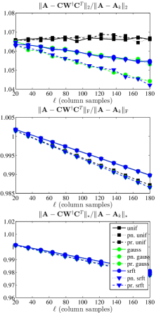
(a) Gnutella, $k=20$

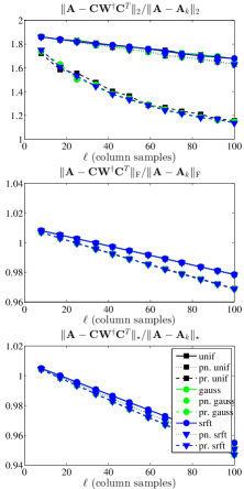
(b) Dexter, $k=8$

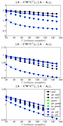
(c) AbaloneD, $\sigma=.15,k=20$

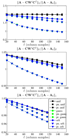
(d) WineS, $\sigma=1,k=20$

Figure 15. The spectral, Frobenius, and trace norm errors (top to bottom, respectively, in each subfigure) of several non-rank-restricted SPSD sketches, including the pinched and prolonged sketches, as a function of the number of columns samples $\ell$, for several datasets. Pinched and prolonged sketches, respectively indicated by “pn.” and “pr.”, are defined in Equations (9) and (10).

Finally, for completeness, we consider the performance of the two projection-based SPSD sketches proposed in [32], and we show how they perform when compared with the sketches we have considered. Recall that the idea of these sketches is to construct low-rank approximations by forming an approximate basis $\mathbf{Q}$ for the top eigenspace of $\mathbf{A}$ and then restricting $\mathbf{A}$ to that eigenspace. In more detail, given a sketching matrix $\mathbf{S},$ form the matrix $\mathbf{Y}=\mathbf{A}\mathbf{S}$ and take the QR decomposition of $\mathbf{Y}$ to obtain $\mathbf{Q},$ a matrix with orthonormal columns. The first sketch, which we eponymously refer to as the pinched sketch, is simply $\mathbf{A}$ pinched to the space spanned by $\mathbf{Q}:$

(9) $$\mathbf{Q}(\mathbf{Q}^{T}\mathbf{A}\mathbf{Q})\mathbf{Q}^{T}.$$

The second sketch, which we refer to as the prolonged sketch, is

(10) $$\mathbf{A}\mathbf{Q}(\mathbf{Q}^{T}\mathbf{A}\mathbf{Q})^{\dagger}\mathbf{Q}^{T}\mathbf{A}.$$

It is clear that the prolonged sketch can be constructed using our SPSD Sketching Model by taking $\mathbf{Q}$ as the sketching matrix. In fact, a stronger statement can be made. As shown in [28], and as stated in Lemma 1 below, it is the case, for any sketching matrix $\mathbf{X},$ that when $\mathbf{C}=\mathbf{A}\mathbf{X}$ and $\mathbf{W}=\mathbf{X}^{T}\mathbf{A}\mathbf{X},$

$$\mathbf{C}\mathbf{W}^{\dagger}\mathbf{C}^{T}=\mathbf{A}^{1/2}\mathbf{P}_{\mathbf{A}^{1/2}\mathbf{X}}\mathbf{A}^{1/2}.$$

By considering the two choices $\mathbf{X}=\mathbf{A}\mathbf{S}$ and $\mathbf{X}=\mathbf{Q}$, we see that in fact the prolonged sketch is exactly the sketch obtained by applying the power method with $q=2:$

$$\mathbf{A}\mathbf{Q}(\mathbf{Q}^{T}\mathbf{A}\mathbf{Q})^{\dagger}\mathbf{Q}^{T}\mathbf{A} =\mathbf{A}^{1/2}\mathbf{P}_{\mathbf{A}^{1/2}\mathbf{Q}}\mathbf{A}^{1/2}$$

$$=\mathbf{A}^{1/2}\mathbf{P}_{\mathbf{A}^{1/2}(\mathbf{A}\mathbf{S})}\mathbf{A}^{1/2}$$

$$=\mathbf{A}^{2}\mathbf{S}(\mathbf{S}^{T}\mathbf{A}^{3}\mathbf{S})^{\dagger}\mathbf{S}^{T}\mathbf{A}^{2}.$$

It follows that the bounds we provide in Section 4 on the performance of sketches obtained using the power method pertain also to prolonged sketches.

In Figure 15, we compare the empirical performances of several of the SPSD sketches considered earlier with their pinched and prolonged variants. Specifically, we plot the errors of pinched and prolonged sketches for several choices of sketching matrices—corresponding to uniform column sampling, gaussian column mixtures, and SRFT-based column mixtures—along with the errors of non-pinched, non-prolonged sketches constructing using the same choices of $\mathbf{S}.$ In the interest of brevity, we provide results only for several of the datasets listed in Table 4, and we consider only the nonfixed-rank variants of the sketches.

Some trends are clear from Figure 15.

• In the spectral norm, the prolonged sketches are considerably more accurate than the pinched and standard sketches for all the datasets considered. Without exception, the prolonged Gaussian and SRFT column-mixture sketches are the most accurate in the spectral norm, of all the sketches considered. Only in the case of the Dexter Linear Kernel is the prolonged uniformly column-sampled sketch nearly as accurate in the spectral norm as the prolonged Gaussian and SRFT sketches. To a lesser extent, the prolonged sketches are also more accurate in the Frobenius and trace norms than the other sketches considered. The increased Frobenius and trace norm accuracy is particularly notable for the two RBF Kernel datasets; again, the prolonged Gaussian and SRFT sketches are considerably more accurate than the prolonged uniformly column-sampled sketches.

• After the prolonged sketches, the pinched Gaussian and SRFT column-mixture sketches exhibit the least spectral, Frobenius, and trace norm errors. Again, however, we see that the pinched uniformly column-sampled sketches are considerably less accurate than the pinched Gaussian and SRFT column-mixture sketches. Particularly in the spectral and Frobenius norms, the pinched uniformly column-sampled sketches are not any more accurate than the basic uniformly column-sampled sketches.

From these considerations, it seems evident that the benefits of pinched and prolonged sketches are most prominent when the spectral norm is the error metric, or when the dataset is an RBF Kernel. In particular, pinched and prolonged sketches are not significantly more accurate (than the sketches considered in the previous subsections) in the Frobenius and trace norms for any of the datasets considered.

It is also evident from Figure 15 that the pinched sketches often have a much slighter increase in accuracy over the basic sketches than do the prolonged sketches. To understand why the pinched sketches are less accurate than the prolonged sketches, observe that the pinched sketches satisfy

$$\mathbf{Q}(\mathbf{Q}^{T}\mathbf{A}\mathbf{Q})\mathbf{Q}^{T} =\mathbf{P}_{\mathbf{A}\mathbf{S}}\mathbf{A}\mathbf{P}_{\mathbf{A}\mathbf{S}}$$

$$=(\mathbf{P}_{\mathbf{A}\mathbf{S}}\mathbf{A}^{1/2})(\mathbf{A}^{1/2}\mathbf{P}_{\mathbf{A}\mathbf{S}}),$$

while, as noted above, the prolonged sketches can be written in the form

$$\mathbf{A}\mathbf{Q}(\mathbf{Q}^{T}\mathbf{A}\mathbf{Q})^{\dagger}\mathbf{Q}^{T}\mathbf{A}=(\mathbf{A}^{1/2}\mathbf{P}_{\mathbf{A}^{3/2}\mathbf{S}})(\mathbf{P}_{\mathbf{A}^{3/2}\mathbf{S}}\mathbf{A}^{1/2}).$$

Thus, pinched and prolonged sketches approximate the square root of $\mathbf{A}$ by projecting, respectively, onto the ranges of $\mathbf{A}\mathbf{S}$ and $\mathbf{A}^{3/2}\mathbf{S}.$ The spectral decay present in $\mathbf{A}$ is increased when $\mathbf{A}$ is raised to a power larger than one; consequently, the range of $\mathbf{A}^{3/2}\mathbf{S}$ is more biased towards the top $k$-dimensional invariant subspace of $\mathbf{A}$ than is the range of $\mathbf{A}\mathbf{S}.$ It follows that the approximate square root used to construct the prolonged sketches more accurately captures the top $k$-dimensional subspace of $\mathbf{A}$ than does that used to construct the pinched sketches.

4. Theoretical Aspects of SPSD Low-rank Approximation

In this section, we present our main theoretical results, which consist of a suite of bounds on the quality of low-rank approximation under several different sketching methods. As mentioned above, these were motivated by our empirical observation that all of the sampling and projection methods we considered perform much better on the SPSD matrices we considered than previous worst-case bounds (e.g., [21, 39, 28]) would suggest. We start in Section 4.1 with deterministic structural conditions for the spectral, Frobenius, and trace norms; and then in Section 4.2 we use these results to provide our bounds for several random sampling and random projection procedures.

4.1. Deterministic Error Bounds for Low-rank SPSD Approximation

In this section, we present three theorems that provide error bounds for the spectral, Frobenius, and trace norm approximation errors under the SPSD Sketching Model of Section 2.2. These are provided in Sections 4.1.1, 4.1.3, and 4.1.5, respectively, and they are followed by several more general remarks in Section 4.1.6. Note that these bounds hold for any, e.g., deterministic or randomized, sketching matrix $\mathbf{S}$. Thus, e.g., one could use them to check, in an a posteriori manner, the quality of a sketching method for which one cannot establish an a priori bound. Rather than doing this, we use these results (in Section 4.2 below) to derive a priori bounds for when the sketching operation consists of common random sampling and random projection algorithms.

Our results are based on the fact, established in [28], that approximations which satisfy our SPSD Sketching Model can be written in terms of a projection onto a subspace of the range of the square root of the matrix being approximated. The following fact appears in the proof of Proposition 1 in [28].

inline]Update this reference to unreleased version in anticipation of changing on arxiv

Lemma 1 ([28]).

Let $\mathbf{A}$ be an SPSD matrix and $\mathbf{S}$ be a conformal sketching matrix. Then when $\mathbf{C}=\mathbf{A}\mathbf{S}$ and $\mathbf{W}=\mathbf{S}^{T}\mathbf{A}\mathbf{S},$ the corresponding low-rank SPSD approximation satisfies

$$\mathbf{C}\mathbf{W}^{\dagger}\mathbf{C}^{T}=\mathbf{A}^{1/2}\mathbf{P}_{\mathbf{A}^{1/2}\mathbf{S}}\mathbf{A}^{1/2}.$$

4.1.1. Spectral Norm Bounds

We start with a bound on the spectral norm of the residual error. Although this result is trivial to prove, given prior work, it highlights several properties that we use in the analysis of our subsequent results.

Theorem 1.

Let $\mathbf{A}$ be an $n\times n$ SPSD matrix with eigenvalue decomposition partitioned as in Equation (1), $\mathbf{S}$ be a sketching matrix of size $n\times\ell$, $q$ be a positive integer, and $\boldsymbol{\Omega}_{1}$ and $\boldsymbol{\Omega}_{2}$ be as defined in Equation (3). Then when $\mathbf{C}=\mathbf{A}^{q}\mathbf{S}$ and $\mathbf{W}=\mathbf{S}^{T}\mathbf{A}^{2q-1}\mathbf{S}$, the corresponding low-rank SPSD approximation satisfies

$$\left\|\mathbf{A}-\mathbf{C}\mathbf{W}^{\dagger}\mathbf{C}^{T}\right\|_{2}\leq\left\|\boldsymbol{\Sigma}_{2}\right\|_{2}+\left\|\boldsymbol{\Sigma}_{2}^{q-1/2}\boldsymbol{\Omega}_{2}\boldsymbol{\Omega}_{1}^{\dagger}\right\|_{2}^{2/(2q-1)},$$

assuming $\boldsymbol{\Omega}_{1}$ has full row rank.

Proof.

Apply Lemma 1 with the sampling matrix $\mathbf{S}^{\prime}=\mathbf{A}^{q-1}\mathbf{S}$ (where, recall, $q\geq 1$) to see that

$$\mathbf{C}\mathbf{W}^{\dagger}\mathbf{C}^{T}=\mathbf{A}^{1/2}\mathbf{P}_{\mathbf{A}^{q-1/2}\mathbf{S}}\mathbf{A}^{1/2}.$$

It follows that

(11) $$\left\|\mathbf{A}-\mathbf{C}\mathbf{W}^{\dagger}\mathbf{C}^{T}\right\|_{2}=\left\|\mathbf{A}^{1/2}\left(\mathbf{I}-\mathbf{P}_{\left(\mathbf{A}^{1/2}\right)^{2q-1}\mathbf{S}}\right)\mathbf{A}^{1/2}\right\|_{2}^{2}.$$

Next, recall that $\boldsymbol{\Omega}_{i}=\mathbf{U}_{i}^{T}\mathbf{S}$ and that $\mathbf{A}^{1/2}$ has eigenvalue decomposition $\mathbf{A}=\mathbf{U}\boldsymbol{\Sigma}^{1/2}\mathbf{U}^{T},$ where

$$\mathbf{U}=\begin{pmatrix}\mathbf{U}_{1}&\mathbf{U}_{2}\end{pmatrix}\text{ and }\boldsymbol{\Sigma}^{1/2}=\begin{pmatrix}\boldsymbol{\Sigma}_{1}^{1/2}&\,\\ \,&\boldsymbol{\Sigma}_{2}^{1/2}\end{pmatrix}.$$

It can be shown ([32, Theorems 9.1 and 9.2]) that, because $\boldsymbol{\Omega}_{1}$ has full row rank,

(12) $$\left\|\mathbf{A}^{1/2}\left(\mathbf{I}-\mathbf{P}_{\left(\mathbf{A}^{1/2}\right)^{2q-1}\mathbf{S}}\right)\mathbf{A}^{1/2}\right\|_{2}^{2}\leq\left(\left\|\left(\boldsymbol{\Sigma}_{2}^{1/2}\right)^{2q-1}\right\|_{2}^{2}+\left\|\left(\boldsymbol{\Sigma}_{2}^{1/2}\right)^{2q-1}\boldsymbol{\Omega}_{2}\boldsymbol{\Omega}_{1}^{\dagger}\right\|_{2}^{2}\right)^{1/(2q-1)}.$$

Equations (11) and (12) imply that

$$\left\|\mathbf{A}-\mathbf{C}\mathbf{W}^{\dagger}\mathbf{C}^{T}\right\|_{2} \leq\left(\left\|\boldsymbol{\Sigma}_{2}^{q-1/2}\right\|_{2}^{2}+\left\|\boldsymbol{\Sigma}_{2}^{q-1/2}\boldsymbol{\Omega}_{2}\boldsymbol{\Omega}_{1}^{\dagger}\right\|_{2}^{2}\right)^{1/(2q-1)}$$

$$\leq\left\|\boldsymbol{\Sigma}_{2}\right\|_{2}+\left\|\boldsymbol{\Sigma}_{2}^{q-1/2}\boldsymbol{\Omega}_{2}\boldsymbol{\Omega}_{1}^{\dagger}\right\|_{2}^{2/(2q-1)}$$

The latter inequality follows from the fact that the $2q-1$ radical function is subadditive when $q\geq 1$ and the identity $\left\|\boldsymbol{\Sigma}_{2}^{q-1/2}\right\|_{2}^{2}=\left\|\boldsymbol{\Sigma}_{2}\right\|_{2}^{2q-1}.$ This establishes the stated bound. ∎

Remark. The assumption that $\boldsymbol{\Omega}_{1}$ has full row rank is very non-trivial. It is, however, satisfied by our algorithms below. See Section 4.1.6 for more details on this point.

Remark. The proof of Theorem 1 proceeds in two steps. The first step relates low-rank approximation of an SPSD matrix $\mathbf{A}$ under the SPSD Sketching Model of Section 2.2 to column sketching (e.g., sampling or projecting) from the square-root of $\mathbf{A}$. A weaker relation of this type was used in [21], but the stronger form that we use here in Equation (11) was first proved in [28]. The second step is to use a deterministic structural result that holds for sampling/projecting from an arbitrary matrix. The structural bound of the form of Equation (12) was originally proven for $q=1$ in [14], where it was applied to the Column Subset Selection Problem. The bound was subsequently improved in [32], where it was applied to a random projection algorithm and extended to apply when $q>1$. Although the analyses of our next two results are more complicated, they follow the same high-level two-step approach.

Before proceeding with the analogous Frobenius and trace norm bounds, we pause to describe a geometric interpretation of this result.

inline]Explain interpretation of $\boldsymbol{\Omega}_{2}\boldsymbol{\Omega}_{1}^{\dagger}$, how it shows up in convergence of power method, and how it being small implies $\mathbf{S}$ is an effective sketching matrix.

4.1.2. A geometric interpretation of the sketching interaction matrix

It is evident from the bound in Theorem 1 that the smaller the spectral norm of the sketching interaction matrix $\boldsymbol{\Omega}_{2}\boldsymbol{\Omega}_{1}^{\dagger},$ the more effective $\mathbf{S}$ is as a sketching matrix. If, additionally, the columns of $\mathbf{S}$ are orthonormal, we can give this norm a natural geometric interpretation as the tangent of the largest angle between the spaces spanned by $\mathbf{S}$ and $\mathbf{U}_{1}.$

To verify our claim, we first recall the definition of the sine between the range spaces of two matrices $\mathbf{M}_{1}$ and $\mathbf{M}_{2}:$

$$\sin^{2}(\mathbf{M}_{1},\mathbf{M}_{2})=\left\|(\mathbf{I}-\mathbf{P}_{\mathbf{M}_{1}})\mathbf{P}_{\mathbf{M}_{2}})\right\|_{2}^{2}.$$

Note that this quantity is not symmetric: it measures how well the range of $\mathbf{M}_{1}$ captures that of $\mathbf{M}_{2}$ [29, Chapter 12]. Since $\mathbf{U}_{1}$ and $\mathbf{S}$ (by assumption here) have orthonormal columns, we see that

$$\sin^{2}(\mathbf{S},\mathbf{U}_{1}) =\left\|(\mathbf{I}-\mathbf{S}\mathbf{S}^{T})\mathbf{U}_{1}\mathbf{U}_{1}^{T}\right\|_{2}^{2}$$

$$=\left\|\mathbf{U}_{1}^{T}(\mathbf{I}-\mathbf{S}\mathbf{S}^{T})\mathbf{U}_{1}\right\|_{2}$$

$$=\left\|\mathbf{I}-\mathbf{U}_{1}^{T}\mathbf{S}\mathbf{S}^{T}\mathbf{U}_{1}\right\|_{2}$$

$$=1-\lambda_{k}(\mathbf{U}_{1}^{T}\mathbf{S}\mathbf{S}^{T}\mathbf{U}_{1})$$

$$=1-\left\|\boldsymbol{\Omega}_{1}^{\dagger}\right\|_{2}^{-2}.$$

The second to last equality holds because $\mathbf{U}_{1}^{T}\mathbf{S}$ has $k$ rows and we assumed it has full row rank. Accordingly, it follows that

$$\tan^{2}(\mathbf{S},\mathbf{U}_{1})=\frac{\sin^{2}(\mathbf{S},\mathbf{U}_{1})}{1-\sin^{2}(\mathbf{S},\mathbf{U}_{1})}=\left\|\boldsymbol{\Omega}_{1}^{\dagger}\right\|_{2}^{2}-1.$$

Now observe that

$$\left\|\boldsymbol{\Omega}_{2}\boldsymbol{\Omega}_{1}^{\dagger}\right\|_{2}^{2} =\left\|(\mathbf{S}^{T}\mathbf{U}_{1})^{\dagger}\mathbf{S}^{T}\mathbf{U}_{2}\mathbf{U}_{2}^{T}\mathbf{S}(\mathbf{U}_{1}^{T}\mathbf{S})^{\dagger}\right\|_{2}$$

$$=\left\|(\mathbf{S}^{T}\mathbf{U}_{1})^{\dagger}(\mathbf{I}-\mathbf{S}^{T}\mathbf{U}_{1}\mathbf{U}_{1}^{T}\mathbf{S})(\mathbf{U}_{1}^{T}\mathbf{S})^{\dagger}\right\|_{2}$$

$$=\left\|(\mathbf{S}^{T}\mathbf{U}_{1})^{\dagger}\right\|_{2}^{2}-1$$

$$=\tan^{2}(\mathbf{S},\mathbf{U}_{1}).$$

The second to last equality holds because of the fact that, for any matrix $\mathbf{M},$

$$\left\|\mathbf{M}^{\dagger}(\mathbf{I}-\mathbf{M}\mathbf{M}^{T})(\mathbf{M}^{T})^{\dagger}\right\|_{2}=\left\|\mathbf{M}^{\dagger}\right\|_{2}^{2}-1;$$

this identity can be established with a routine SVD argument.

Thus, when $\mathbf{S}$ has orthonormal columns and $\mathbf{U}_{1}^{T}\mathbf{S}$ has full row-rank, $\left\|\boldsymbol{\Omega}_{2}\boldsymbol{\Omega}_{1}\right\|_{2}$ is the tangent of the largest angle between the range of $\mathbf{S}$ and the eigenspace spanned by $\mathbf{U}_{1}.$ If $\mathbf{U}_{1}^{T}\mathbf{S}$ does not have full row-rank, then our derivation above shows that $\sin^{2}(\mathbf{S},\mathbf{U}_{1})=1,$ meaning that there is a vector in the eigenspace spanned by $\mathbf{U}_{1}$ which has no component in the space spanned by the sketching matrix $\mathbf{S}.$

We note that $\tan(\mathbf{S},\mathbf{U}_{1})$ also arises in the classical bounds on the convergence of the orthogonal iteration algorithm for approximating invariant subspaces of a matrix (see, e.g. [29, Theorem 8.2.2]).

4.1.3. Frobenius Norm Bounds

Next, we state and prove the following bound on the Frobenius norm of the residual error. The proof parallels that for the spectral norm bound, in that we divide it into two analogous parts, but the analysis is somewhat more complex.

The multiplicative eigengap $\gamma=\lambda_{k+1}(\mathbf{A})/\lambda_{k}(\mathbf{A})$ that appears in the statement of this theorem predicts the effect of using the power method when constructing sketches. Specifically, the additional errors of sketches constructed using $\mathbf{C}=\mathbf{A}^{q}\mathbf{S}$ are at least a factor of $\gamma^{q-1}$ times smaller than those constructed using $\mathbf{C}=\mathbf{A}\mathbf{S}.$

Theorem 2.

Let $\mathbf{A}$ be an $n\times n$ SPSD matrix with eigenvalue decomposition partitioned as in Equation (1), $\mathbf{S}$ be a sketching matrix of size $n\times\ell$, $q$ be a positive integer, $\boldsymbol{\Omega}_{1}$ and $\boldsymbol{\Omega}_{2}$ be as defined in Equation (3), and define

$$\gamma=\frac{\lambda_{k+1}(\mathbf{A})}{\lambda_{k}(\mathbf{A})}.$$

Then when $\mathbf{C}=\mathbf{A}^{q}\mathbf{S}$ and $\mathbf{W}=\mathbf{S}^{T}\mathbf{A}^{2q-1}\mathbf{S}$, the corresponding low-rank SPSD approximation satisfies

$$\left\|\mathbf{A}-\mathbf{C}\mathbf{W}^{\dagger}\mathbf{C}^{T}\right\|_{\mathrm{F}}\leq\left\|\boldsymbol{\Sigma}_{2}\right\|_{\mathrm{F}}+\gamma^{q-1}\left\|\boldsymbol{\Sigma}_{2}^{1/2}\boldsymbol{\Omega}_{2}\boldsymbol{\Omega}_{1}^{\dagger}\right\|_{2}\cdot\left(\sqrt{2\operatorname{Tr}\left(\boldsymbol{\Sigma}_{2}\right)}+\gamma^{q-1}\left\|\boldsymbol{\Sigma}_{2}^{1/2}\boldsymbol{\Omega}_{2}\boldsymbol{\Omega}_{1}^{\dagger}\right\|_{\mathrm{F}}\right),$$

assuming $\boldsymbol{\Omega}_{1}$ has full row rank.

Proof.

Apply Lemma 1 with the sampling matrix $\mathbf{S}^{\prime}=\mathbf{A}^{q-1}\mathbf{S}$ to see that

$$\mathbf{C}\mathbf{W}^{\dagger}\mathbf{C}^{T}=\mathbf{A}^{1/2}\mathbf{P}_{\mathbf{A}^{q-1/2}\mathbf{S}}\mathbf{A}^{1/2}.$$

It follows that

$$\left\|\mathbf{A}-\mathbf{C}\mathbf{W}^{\dagger}\mathbf{C}^{T}\right\|_{\mathrm{F}}=\left\|\mathbf{A}^{1/2}\left(\mathbf{I}-\mathbf{P}_{\mathbf{A}^{q-1/2}\mathbf{S}}\right)\mathbf{A}^{1/2}\right\|_{\mathrm{F}}.$$

To bound this quantity, we first use the unitary invariance of the Frobenius norm and the fact that

$$\mathbf{P}_{\mathbf{A}^{q-1/2}\mathbf{S}}=\mathbf{U}\mathbf{P}_{\boldsymbol{\Sigma}^{q-1/2}\mathbf{U}^{T}\mathbf{S}}\mathbf{U}^{T}$$

to obtain

$$E:=\left\|\mathbf{A}^{1/2}\left(\mathbf{I}-\mathbf{P}_{\mathbf{A}^{q-1/2}\mathbf{S}}\right)\mathbf{A}^{1/2}\right\|_{\mathrm{F}}=\left\|\boldsymbol{\Sigma}^{1/2}\left(\mathbf{I}-\mathbf{P}_{\boldsymbol{\Sigma}^{q-1/2}\mathbf{U}^{T}\mathbf{S}}\right)\boldsymbol{\Sigma}^{1/2}\right\|_{\mathrm{F}}^{2}.$$

Then we take

(13) $$\mathbf{Z}=\boldsymbol{\Sigma}^{q-1/2}\mathbf{U}^{T}\mathbf{S}\boldsymbol{\Omega}_{1}^{\dagger}\boldsymbol{\Sigma}_{1}^{-(q-1/2)}=\begin{pmatrix}\mathbf{I}\\ \mathbf{F}\end{pmatrix},$$

where $\mathbf{I}\in\mathbb{R}^{k\times k}$ and $\mathbf{F}\in\mathbb{R}^{n-k\times k}$ is given by $\mathbf{F}=\boldsymbol{\Sigma}_{2}^{q-1/2}\boldsymbol{\Omega}_{2}\boldsymbol{\Omega}_{1}^{\dagger}\boldsymbol{\Sigma}_{1}^{-(q-1/2)}.$ The latter equality in Equation (13) holds because of our assumption that $\boldsymbol{\Omega}_{1}$ has full row rank. Since the range of $\mathbf{Z}$ is contained in the range of $\boldsymbol{\Sigma}^{q-1/2}\mathbf{U}^{T}\mathbf{S},$

$$E\leq\left\|\boldsymbol{\Sigma}^{1/2}(\mathbf{I}-\mathbf{P}_{\mathbf{Z}})\boldsymbol{\Sigma}^{1/2}\right\|_{\mathrm{F}}^{2}.$$

By construction, $\mathbf{Z}$ has full column rank, thus $\mathbf{Z}(\mathbf{Z}^{T}\mathbf{Z})^{-1/2}$ is an orthonormal basis for the span of $\mathbf{Z}$, and

$$\mathbf{I}-\mathbf{P}_{\mathbf{Z}} =\mathbf{I}-\mathbf{Z}(\mathbf{Z}^{T}\mathbf{Z})^{-1}\mathbf{Z}^{T}=\mathbf{I}-\begin{pmatrix}\mathbf{I}\\ \mathbf{F}\end{pmatrix}(\mathbf{I}+\mathbf{F}^{T}\mathbf{F})^{-1}\begin{pmatrix}\mathbf{I}&\mathbf{F}^{T}\end{pmatrix}$$

(14) $$=\begin{pmatrix}\mathbf{I}-(\mathbf{I}+\mathbf{F}^{T}\mathbf{F})^{-1}&-(\mathbf{I}+\mathbf{F}^{T}\mathbf{F})^{-1}\mathbf{F}^{T}\\ -\mathbf{F}(\mathbf{I}+\mathbf{F}^{T}\mathbf{F})^{-1}&\mathbf{I}-\mathbf{F}(\mathbf{I}+\mathbf{F}^{T}\mathbf{F})^{-1}\mathbf{F}^{T}\end{pmatrix}.$$

This implies that

(15) $$\begin{split}E&\leq\left\|\boldsymbol{\Sigma}^{1/2}\begin{pmatrix}\mathbf{I}-(\mathbf{I}+\mathbf{F}^{T}\mathbf{F})^{-1}&-(\mathbf{I}+\mathbf{F}^{T}\mathbf{F})^{-1}\mathbf{F}^{T}\\ -\mathbf{F}(\mathbf{I}+\mathbf{F}^{T}\mathbf{F})^{-1}&\mathbf{I}-\mathbf{F}(\mathbf{I}+\mathbf{F}^{T}\mathbf{F})^{-1}\mathbf{F}^{T}\end{pmatrix}\boldsymbol{\Sigma}^{1/2}\right\|_{\mathrm{F}}^{2}\\ &=\left\|\boldsymbol{\Sigma}_{1}^{1/2}\big{(}\mathbf{I}-(\mathbf{I}+\mathbf{F}^{T}\mathbf{F})^{-1}\big{)}\boldsymbol{\Sigma}_{1}^{1/2}\right\|_{\mathrm{F}}^{2}+2\left\|\boldsymbol{\Sigma}_{1}^{1/2}(\mathbf{I}+\mathbf{F}^{T}\mathbf{F})^{-1}\mathbf{F}^{T}\boldsymbol{\Sigma}_{2}^{1/2}\right\|_{\mathrm{F}}^{2}\\ &\quad+\left\|\boldsymbol{\Sigma}_{2}^{1/2}\big{(}\mathbf{I}-\mathbf{F}(\mathbf{I}+\mathbf{F}^{T}\mathbf{F})^{-1}\mathbf{F}^{T}\big{)}\boldsymbol{\Sigma}_{2}^{1/2}\right\|_{\mathrm{F}}^{2}\\ &:=T_{1}+T_{2}+T_{3}.\end{split}$$

Next, we provide bounds for $T_{1}$, $T_{2}$, and $T_{3}$. Using the fact that $\mathbf{0}\preceq\mathbf{I}-\mathbf{F}(\mathbf{I}+\mathbf{F}^{T}\mathbf{F})^{-1}\mathbf{F}^{T}\preceq\mathbf{I},$ we can bound $T_{3}$ with

$$T_{3}\leq\left\|\boldsymbol{\Sigma}_{2}\right\|_{\mathrm{F}}^{2}.$$

Likewise, the fact that $\mathbf{I}-(\mathbf{I}+\mathbf{F}^{T}\mathbf{F})^{-1}\preceq\mathbf{F}^{T}\mathbf{F}$ (easily seen with an SVD) implies that we can bound $T_{1}$ as

$$T_{1} \leq\left\|\boldsymbol{\Sigma}_{1}^{1/2}\mathbf{F}^{T}\mathbf{F}\boldsymbol{\Sigma}_{1}^{1/2}\right\|_{\mathrm{F}}^{2}\leq\left\|\mathbf{F}\boldsymbol{\Sigma}_{1}^{1/2}\right\|_{2}^{2}\left\|\mathbf{F}\boldsymbol{\Sigma}_{1}^{1/2}\right\|_{\mathrm{F}}^{2}$$

$$=\left\|\boldsymbol{\Sigma}_{2}^{q-1/2}\boldsymbol{\Omega}_{2}\boldsymbol{\Omega}_{1}^{\dagger}\boldsymbol{\Sigma}_{1}^{-(q-1)}\right\|_{2}^{2}\left\|\boldsymbol{\Sigma}_{2}^{q-1/2}\boldsymbol{\Omega}_{2}\boldsymbol{\Omega}_{1}^{\dagger}\boldsymbol{\Sigma}_{1}^{-(q-1)}\right\|_{\mathrm{F}}^{2}$$

$$\leq\left\|\boldsymbol{\Sigma}_{2}^{q-1}\right\|_{2}^{4}\left\|\boldsymbol{\Sigma}_{1}^{-(q-1)}\right\|_{2}^{4}\left\|\boldsymbol{\Sigma}_{2}^{1/2}\boldsymbol{\Omega}_{2}\boldsymbol{\Omega}_{1}^{\dagger}\right\|_{2}^{2}\left\|\boldsymbol{\Sigma}_{2}^{1/2}\boldsymbol{\Omega}_{2}\boldsymbol{\Omega}_{1}^{\dagger}\right\|_{\mathrm{F}}^{2}$$

$$=(\left\|\boldsymbol{\Sigma}_{2}\right\|_{2}\left\|\boldsymbol{\Sigma}_{1}^{-1}\right\|_{2})^{4(q-1)}\left\|\boldsymbol{\Sigma}_{2}^{1/2}\boldsymbol{\Omega}_{2}\boldsymbol{\Omega}_{1}^{\dagger}\right\|_{2}^{2}\left\|\boldsymbol{\Sigma}_{2}^{1/2}\boldsymbol{\Omega}_{2}\boldsymbol{\Omega}_{1}^{\dagger}\right\|_{\mathrm{F}}^{2}$$

$$=\left(\frac{\lambda_{k+1}(\mathbf{A})}{\lambda_{k}(\mathbf{A})}\right)^{4(q-1)}\left\|\boldsymbol{\Sigma}_{2}^{1/2}\boldsymbol{\Omega}_{2}\boldsymbol{\Omega}_{1}^{\dagger}\right\|_{2}^{2}\left\|\boldsymbol{\Sigma}_{2}^{1/2}\boldsymbol{\Omega}_{2}\boldsymbol{\Omega}_{1}^{\dagger}\right\|_{\mathrm{F}}^{2}.$$

We proceed to bound $T_{2}$ by using the estimate

(16) $$T_{2}\leq 2\left\|\boldsymbol{\Sigma}_{1}^{1/2}(\mathbf{I}+\mathbf{F}^{T}\mathbf{F})^{-1}\mathbf{F}^{T}\right\|_{2}^{2}\left\|\boldsymbol{\Sigma}_{2}^{1/2}\right\|_{\mathrm{F}}^{2}.$$

To develop the term involving a spectral norm, observe that for any SPSD matrix $\mathbf{M}$ with eigenvalue decomposition $\mathbf{M}=\mathbf{V}\mathbf{D}\mathbf{V}^{T},$

$$(\mathbf{I}+\mathbf{M})^{-1}\mathbf{M}(\mathbf{I}+\mathbf{M})^{-1} =(\mathbf{V}\mathbf{V}^{T}+\mathbf{V}\mathbf{D}\mathbf{V}^{T})^{-1}\mathbf{V}\mathbf{D}\mathbf{V}^{T}(\mathbf{V}\mathbf{V}^{T}+\mathbf{V}\mathbf{D}\mathbf{V}^{T})^{-1}$$

$$=\mathbf{V}(\mathbf{I}+\mathbf{D})^{-1}\mathbf{D}(\mathbf{I}+\mathbf{D})^{-1}\mathbf{V}^{T}$$

$$\preceq\mathbf{V}\mathbf{D}\mathbf{V}^{T}=\mathbf{M}.$$

It follows that

$$\left\|\boldsymbol{\Sigma}_{1}^{1/2}(\mathbf{I}+\mathbf{F}^{T}\mathbf{F})^{-1}\mathbf{F}^{T}\right\|_{2}^{2} =\left\|\boldsymbol{\Sigma}_{1}^{1/2}(\mathbf{I}+\mathbf{F}^{T}\mathbf{F})^{-1}\mathbf{F}^{T}\mathbf{F}(\mathbf{I}+\mathbf{F}^{T}\mathbf{F})^{-1}\boldsymbol{\Sigma}_{1}^{1/2}\right\|_{2}$$

$$\leq\left\|\boldsymbol{\Sigma}_{1}^{1/2}\mathbf{F}^{T}\mathbf{F}\boldsymbol{\Sigma}_{1}^{1/2}\right\|_{2}=\left\|\mathbf{F}\boldsymbol{\Sigma}_{1}^{1/2}\right\|_{2}^{2}$$

$$=\left\|\boldsymbol{\Sigma}_{2}^{q-1/2}\boldsymbol{\Omega}_{2}\boldsymbol{\Omega}_{1}^{\dagger}\boldsymbol{\Sigma}_{1}^{-(q-1)}\right\|_{2}^{2}$$

$$\leq\left\|\boldsymbol{\Sigma}_{2}^{q-1}\right\|_{2}^{2}\left\|\boldsymbol{\Sigma}_{1}^{-(q-1)}\right\|_{2}^{2}\left\|\boldsymbol{\Sigma}_{2}^{1/2}\boldsymbol{\Omega}_{2}\boldsymbol{\Omega}_{1}^{\dagger}\right\|_{2}^{2}$$

$$=\left(\frac{\lambda_{k+1}(\mathbf{A})}{\lambda_{k}(\mathbf{A})}\right)^{2(q-1)}\left\|\boldsymbol{\Sigma}_{2}^{1/2}\boldsymbol{\Omega}_{2}\boldsymbol{\Omega}_{1}^{\dagger}\right\|_{2}^{2}.$$

Using this estimate in Equation (16), we conclude that

$$T_{2}\leq 2\left(\frac{\lambda_{k+1}(\mathbf{A})}{\lambda_{k}(\mathbf{A})}\right)^{2(q-1)}\left\|\boldsymbol{\Sigma}_{2}^{1/2}\boldsymbol{\Omega}_{2}\boldsymbol{\Omega}_{1}^{\dagger}\right\|_{2}^{2}\left\|\boldsymbol{\Sigma}_{2}^{1/2}\right\|_{\mathrm{F}}^{2}.$$

Combining our estimates for $T_{1},$ $T_{2},$ and $T_{3}$ with Equation (15) gives

$$\begin{split}E&=\left\|\mathbf{A}^{1/2}\left(\mathbf{I}-\mathbf{P}_{\mathbf{A}^{q-1/2}\mathbf{S}}\right)\mathbf{A}^{1/2}\right\|_{\mathrm{F}}\\ &\leq\left\|\boldsymbol{\Sigma}_{2}\right\|_{\mathrm{F}}^{2}+\left(\frac{\lambda_{k+1}(\mathbf{A})}{\lambda_{k}(\mathbf{A})}\right)^{2(q-1)}\left\|\boldsymbol{\Sigma}_{2}^{1/2}\boldsymbol{\Omega}_{2}\boldsymbol{\Omega}_{1}^{\dagger}\right\|_{2}^{2}\cdot\left(2\left\|\boldsymbol{\Sigma}_{2}^{1/2}\right\|_{\mathrm{F}}^{2}+\left(\frac{\lambda_{k+1}(\mathbf{A})}{\lambda_{k}(\mathbf{A})}\right)^{2(q-1)}\left\|\boldsymbol{\Sigma}_{2}^{1/2}\boldsymbol{\Omega}_{2}\boldsymbol{\Omega}_{1}^{\dagger}\right\|_{\mathrm{F}}^{2}\right).\end{split}$$

The claimed bound follows by identifying $\gamma$ and applying the subadditivity of the square-root function:

$$E\leq\left\|\boldsymbol{\Sigma}_{2}\right\|_{\mathrm{F}}+\gamma^{q-1}\left\|\boldsymbol{\Sigma}_{2}^{1/2}\boldsymbol{\Omega}_{2}\boldsymbol{\Omega}_{1}^{\dagger}\right\|_{2}\cdot\left(\sqrt{2\operatorname{Tr}\left(\boldsymbol{\Sigma}_{2}\right)}+\gamma^{q-1}\left\|\boldsymbol{\Sigma}_{2}^{1/2}\boldsymbol{\Omega}_{2}\boldsymbol{\Omega}_{1}^{\dagger}\right\|_{\mathrm{F}}\right).$$

∎

Remark. The quality of approximation guarantee provided by Theorem 2 depends on the quantities $\left\|\boldsymbol{\Sigma}_{2}^{1/2}\boldsymbol{\Omega}_{2}\boldsymbol{\Omega}_{1}^{\dagger}\right\|_{2}$ and $\left\|\boldsymbol{\Sigma}_{2}^{1/2}\boldsymbol{\Omega}_{2}\boldsymbol{\Omega}_{1}^{\dagger}\right\|_{\mathrm{F}}$; these quantities reflect the extent to which the sketching matrix is aligned with the eigenspaces of $\mathbf{A}.$ As we will see in Section 4.2, the degree to which we can bound each of these for different sketching procedures is slightly different. The dependence on $\gamma$ captures the facts that the power method is effective only when there is spectral decay, and that larger gaps between the $k$ and $k+1$ eigenvalues lead to smaller errors when the power method is used.

As before, we pause to describe a geometric interpretation of this result.

4.1.4. Another geometric interpretation of the sketching interaction matrix

Just as the spectral norm of the spectral interaction matrix is the tangent of the largest angle between the range of the sketching matrix and the dominant $k$-dimensional eigenspace of $\mathbf{A}$, the Frobenius norm of the spectral interaction matrix has a geometric interpretation. To see this, recall that the principal angles between the ranges of the matrices $\mathbf{S}$ and $\mathbf{U}_{1}$ are defined recursively by

$$\cos(\theta_{i})=\mathbf{u}_{i}^{T}\mathbf{v}_{i}=\max_{\begin{subarray}{c}\left\|\mathbf{u}\right\|_{2}=1\\ \mathbf{u}\in\mathcal{R}(\mathbf{S})\\ \mathbf{u}_{i}\perp\mathbf{u}_{1},\ldots,\mathbf{u}_{i-1}\end{subarray}}\max_{\begin{subarray}{c}\left\|\mathbf{v}\right\|_{2}=1\\ \mathbf{v}\in\mathcal{R}(\mathbf{U}_{1})\\ \mathbf{v}_{i}\perp\mathbf{v}_{1},\ldots,\mathbf{v}_{i-1}\end{subarray}}\mathbf{v}^{T}\mathbf{u};$$

satisfy $0\leq\theta_{1}\leq\ldots\leq\theta_{k}\leq\pi/2;$ and further, since $\mathbf{S}$ and $\mathbf{U}_{1}$ have orthonormal columns, $\cos(\theta_{i})=\sigma_{i}(\mathbf{U}_{1}^{T}\mathbf{S})$ [29, Chapter 12]. Specifically, when $\mathbf{S}$ has orthonormal columns and $\mathbf{U}_{1}^{T}\mathbf{S}$ has full row-rank, $\|\boldsymbol{\Omega}_{2}\boldsymbol{\Omega}_{1}^{\dagger}\|_{\mathrm{F}}$ is the sum of the squared tangents of the principal angles between the range of the sketching matrix and the dominant $k$-dimensional eigenspace of $\mathbf{A}$. Thus, this quantity is a more stringent measure of how well the sketching matrix captures the dominant eigenspaces of $\mathbf{A}.$

The proof of this claim hinges on the fact that, for any matrix $\mathbf{M},$

$$\operatorname{Tr}\left(\mathbf{M}^{\dagger}(\mathbf{I}-\mathbf{M}\mathbf{M}^{T})(\mathbf{M}^{T})^{\dagger}\right)=\operatorname{Tr}\left((\mathbf{M}^{T}\mathbf{M})^{\dagger}\right)-\mbox{rank}(\mathbf{M}),$$

as can be readily verified with an SVD argument. From this observation, we have that

$$\left\|\boldsymbol{\Omega}_{2}\boldsymbol{\Omega}_{1}^{\dagger}\right\|_{\mathrm{F}}^{2} =\operatorname{Tr}\left((\mathbf{S}^{T}\mathbf{U}_{1})^{\dagger}\mathbf{S}^{T}\mathbf{U}_{2}\mathbf{U}_{2}^{T}\mathbf{S}(\mathbf{U}_{1}^{T}\mathbf{S})^{\dagger}\right)$$

$$=\operatorname{Tr}\left((\mathbf{S}^{T}\mathbf{U}_{1})^{\dagger}(\mathbf{I}-\mathbf{S}^{T}\mathbf{U}_{1}\mathbf{U}_{1}^{T}\mathbf{S})(\mathbf{U}_{1}^{T}\mathbf{S})^{\dagger}\right)$$

$$=\operatorname{Tr}\left((\boldsymbol{\Omega}_{1}\boldsymbol{\Omega}_{1}^{T})^{\dagger}\right)-k=\left\|\boldsymbol{\Omega}_{1}^{\dagger}\right\|_{\mathrm{F}}^{2}-k$$

$$=\sum\nolimits_{i=1}^{k}(\sigma_{i}^{-2}(\mathbf{U}_{1}^{T}\mathbf{S})-1)=\sum\nolimits_{i=1}^{k}(\cos^{-2}(\theta_{i})-1)$$

$$=\sum\nolimits_{i=1}^{k}\tan^{2}(\theta_{i}).$$

Remark. To obtain a greater understanding of the additional error term in Theorem 2, assume that $\mathbf{S}$ is a particularly effective sketching matrix, so that $\left\|\boldsymbol{\Omega}_{2}\boldsymbol{\Omega}_{1}^{\dagger}\right\|_{2}=\mathrm{O}(1).$ Then

$$\left\|\boldsymbol{\Sigma}_{2}^{1/2}\boldsymbol{\Omega}_{2}\boldsymbol{\Omega}_{1}^{\dagger}\right\|_{2}=\mathrm{O}\left(\left\|\boldsymbol{\Sigma}_{2}\right\|_{2}^{1/2}\right)\quad\text{ and }\quad\sqrt{2\operatorname{Tr}\left(\boldsymbol{\Sigma}_{2}\right)}+\left\|\boldsymbol{\Sigma}_{2}^{1/2}\boldsymbol{\Omega}_{2}\boldsymbol{\Omega}_{1}^{\dagger}\right\|_{\mathrm{F}}=\mathrm{O}\left(\left\|\boldsymbol{\Sigma}_{2}\right\|_{\star}^{1/2}\right),$$

so the theorem guarantees that the additional error is on the order of $\sqrt{\left\|\boldsymbol{\Sigma}_{2}\right\|_{2}\left\|\boldsymbol{\Sigma}_{2}\right\|_{\star}}.$ This is an upper bound on the optimal Frobenius error:

$$\left\|\boldsymbol{\Sigma}_{2}\right\|_{\mathrm{F}}\leq\sqrt{\left\|\boldsymbol{\Sigma}_{2}\right\|_{2}\left\|\boldsymbol{\Sigma}_{2}\right\|_{\star}}.$$

We see, in particular, that if the residual spectrum is flat, i.e. $\lambda_{k+1}(\mathbf{A})=\cdots=\lambda_{n}(\mathbf{A}),$ then equality holds and the additional error is on the scale of the optimal error.

inline]It’s worth asking if this bound can be replaced with the optimal error itself.

4.1.5. Trace Norm Bounds

Finally, we state and prove the following bound on the trace norm of the residual error. The proof method is analogous to that for the spectral and Frobenius norm bounds.

As in the case of the Frobenius norm error, we see that the multiplicative eigengap $\gamma=\lambda_{k+1}(\mathbf{A})/\lambda_{k}(\mathbf{A})$ predicts the effect of using the power method when constructing sketches: the additional errors of sketches constructed using $\mathbf{C}=\mathbf{A}^{q}\mathbf{S}$ are a factor of $\gamma^{2(q-1)}$ times smaller than the additional errrors of those constructed using $\mathbf{C}=\mathbf{A}\mathbf{S}.$

Theorem 3.

Let $\mathbf{A}$ be an $n\times n$ SPSD matrix with eigenvalue decomposition partitioned as in Equation (1), $\mathbf{S}$ be a sketching matrix of size $n\times\ell$, $q$ be a positive integer, $\boldsymbol{\Omega}_{1}$ and $\boldsymbol{\Omega}_{2}$ be as defined in Equation (3), and define

$$\gamma=\frac{\lambda_{k+1}(\mathbf{A})}{\lambda_{k}(\mathbf{A})}.$$

Then when $\mathbf{C}=\mathbf{A}^{q}\mathbf{S}$ and $\mathbf{W}=\mathbf{S}^{T}\mathbf{A}^{2q-1}\mathbf{S}$, the corresponding low-rank SPSD approximation satisfies

$$\left\|\mathbf{A}-\mathbf{C}\mathbf{W}^{\dagger}\mathbf{C}^{T}\right\|_{\star}\leq\operatorname{Tr}\left(\boldsymbol{\Sigma}_{2}\right)+\gamma^{2(q-1)}\left\|\boldsymbol{\Sigma}_{2}^{1/2}\boldsymbol{\Omega}_{2}\boldsymbol{\Omega}_{1}^{\dagger}\right\|_{\mathrm{F}}^{2},$$

assuming $\boldsymbol{\Omega}_{1}$ has full row rank.

Proof.

Since $\mathbf{A}-\mathbf{C}\mathbf{W}^{\dagger}\mathbf{C}^{T}=\mathbf{A}^{1/2}(\mathbf{I}-\mathbf{P}_{\mathbf{A}^{q-1/2}\mathbf{S}})\mathbf{A}^{1/2}\succeq\mathbf{0},$ its trace norm simplifies to its trace. Thus

$$\left\|\mathbf{A}-\mathbf{C}\mathbf{W}^{\dagger}\mathbf{C}^{T}\right\|_{\star} =\operatorname{Tr}\left(\mathbf{A}-\mathbf{C}\mathbf{W}^{\dagger}\mathbf{C}^{T}\right)=\operatorname{Tr}\left(\boldsymbol{\Sigma}^{1/2}\left(\mathbf{I}-\mathbf{P}_{\boldsymbol{\Sigma}^{q-1/2}\mathbf{S}}\right)\boldsymbol{\Sigma}^{1/2}\right)$$

$$\leq\operatorname{Tr}\left(\boldsymbol{\Sigma}^{1/2}(\mathbf{I}-\mathbf{P}_{\mathbf{Z}})\boldsymbol{\Sigma}^{1/2}\right),$$

where $\mathbf{Z}=\begin{pmatrix}\mathbf{I}\\ \mathbf{F}\end{pmatrix}$ is defined in Equation (13). The expression for $\mathbf{I}-\mathbf{P}_{\mathbf{Z}}$ given in Equation (14) implies that

$$\operatorname{Tr}\left(\boldsymbol{\Sigma}^{1/2}(\mathbf{I}-\mathbf{P}_{\mathbf{Z}})\boldsymbol{\Sigma}^{1/2}\right)=\operatorname{Tr}\left(\boldsymbol{\Sigma}_{1}^{1/2}(\mathbf{I}-(\mathbf{I}+\mathbf{F}^{T}\mathbf{F})^{-1})\boldsymbol{\Sigma}_{1}^{1/2}\right)+\operatorname{Tr}\left(\boldsymbol{\Sigma}_{2}^{1/2}(\mathbf{I}-\mathbf{F}(\mathbf{I}+\mathbf{F}^{T}\mathbf{F})^{-1}\mathbf{F}^{T})\boldsymbol{\Sigma}_{2}^{1/2}\right).$$

Recall the estimate $\mathbf{I}-(\mathbf{I}+\mathbf{F}^{T}\mathbf{F})^{-1}\preceq\mathbf{F}^{T}\mathbf{F}$ and the basic estimate $\mathbf{I}-\mathbf{F}(\mathbf{I}+\mathbf{F}^{T}\mathbf{F})^{-1}\mathbf{F}^{T}\preceq\mathbf{I}.$ Together these imply that

$$\operatorname{Tr}\left(\boldsymbol{\Sigma}^{1/2}(\mathbf{I}-\mathbf{P}_{\mathbf{Z}})\boldsymbol{\Sigma}^{1/2}\right) \leq\operatorname{Tr}\left(\boldsymbol{\Sigma}_{1}^{1/2}\mathbf{F}^{T}\mathbf{F}\boldsymbol{\Sigma}_{1}^{1/2}\right)+\operatorname{Tr}\left(\boldsymbol{\Sigma}_{2}\right)$$

$$=\operatorname{Tr}\left(\boldsymbol{\Sigma}_{2}\right)+\left\|\boldsymbol{\Sigma}_{2}^{q-1/2}\boldsymbol{\Omega}_{2}\boldsymbol{\Omega}_{1}^{\dagger}\boldsymbol{\Sigma}_{1}^{-(q-1)}\right\|_{\mathrm{F}}^{2}$$

$$\leq\operatorname{Tr}\left(\boldsymbol{\Sigma}_{2}\right)+\left\|\boldsymbol{\Sigma}_{2}^{q-1}\right\|_{2}^{2}\left\|\boldsymbol{\Sigma}_{1}^{-(q-1)}\right\|_{2}^{2}\left\|\boldsymbol{\Sigma}_{2}^{1/2}\boldsymbol{\Omega}_{2}\boldsymbol{\Omega}_{1}^{\dagger}\right\|_{\mathrm{F}}^{2}$$

$$=\operatorname{Tr}\left(\boldsymbol{\Sigma}_{2}\right)+\gamma^{2(q-1)}\left\|\boldsymbol{\Sigma}_{2}^{1/2}\boldsymbol{\Omega}_{2}\boldsymbol{\Omega}_{1}^{\dagger}\right\|_{\mathrm{F}}^{2}.$$

The first equality follows from substituting the definition of $\mathbf{F}$ and identifying the squared Frobenius norm. The last equality follows from identifying $\gamma.$ We have established the claimed bound.

∎

Remark. Since the identity $\left\|\mathbf{X}\right\|_{\mathrm{F}}^{2}=\left\|\mathbf{X}\mathbf{X}^{T}\right\|_{\star}$ holds for any matrix $\mathbf{X},$ the squared Frobenius norm term present in the deterministic error bound for the trace norm error is on the scale of $\left\|\boldsymbol{\Sigma}_{2}\right\|_{\star}$ when $\big{\|}\boldsymbol{\Omega}_{2}\boldsymbol{\Omega}_{1}^{\dagger}\big{\|}_{2}$ is $\mathrm{O}(1).$

4.1.6. Additional Remarks on Our Deterministic Structural Results.

Before applying these deterministic structural results in particular randomized algorithmic settings, we pause to make several additional remarks about these three theorems.

First, for some randomized sampling schemes, it may be difficult to obtain a sharp bound on $\big{\|}\boldsymbol{\Omega}_{2}\boldsymbol{\Omega}_{1}^{\dagger}\big{\|}_{\xi}$ for $\xi=2,F$. In these situations, the bounds on the excess error supplied by Theorems 1, 2, and 3 may be quite pessimistic. On the other hand, since $\mathbf{A}-\mathbf{C}\mathbf{W}^{\dagger}\mathbf{C}^{T}=\mathbf{A}^{1/2}(\mathbf{I}-\mathbf{P}_{\left(\mathbf{A}^{1/2}\right)^{2q-1}\mathbf{S}})\mathbf{A}^{1/2}$, it follows that $\mathbf{0}\preceq\mathbf{A}-\mathbf{C}\mathbf{W}^{\dagger}\mathbf{C}^{T}\preceq\mathbf{A}$. This implies that the errors of any approximation generated used the SPSD Sketching Model, deterministic or randomized, satisfy at least the crude bound $\left\|\mathbf{A}-\mathbf{C}\mathbf{W}^{\dagger}\mathbf{C}^{T}\right\|_{\xi}\leq\left\|\mathbf{A}\right\|_{\xi}$.

Second, we emphasize that these theorems are deterministic structural results that bound the additional error (beyond that of the optimal rank-$k$ approximation) of low-rank approximations which follow our SPSD sketching model. That is, there is no randomness in their statement or analysis. In particular, these bounds hold for deterministic as well as randomized sketching matrices $\mathbf{S}$. In the latter case, the randomness enters only through $\mathbf{S}$, and one needs to show that the condition that $\boldsymbol{\Omega}_{1}$ has full row rank is satisfied with high probability; conditioned on this, the quality of the bound is determined by terms that depend on how the sketching matrix interacts with the subspace structure of the matrix $\mathbf{A}$.

In particular, we remind the reader that (although it is beyond the scope of this paper to explore this point in detail) these deterministic structural results could be used to check, in an a posteriori manner, the quality of a sketching method for which one cannot establish an a priori bound.

Third, we also emphasize that the assumption that $\boldsymbol{\Omega}_{1}$ has full row rank (equivalently, that $\tan(\mathbf{S},\mathbf{U}_{1})<\infty$) is very non-trivial; and that it is false, in worst-case at least and for non-trivial parameter values, for common sketching methods such as uniform sampling. To see that some version of leverage-based sampling is needed to ensure this condition, recall that $\mathbf{U}_{1}^{T}\mathbf{U}_{1}=\mathbf{I}$ and thus that $\boldsymbol{\Omega}_{1}\boldsymbol{\Omega}_{1}^{T}=\mathbf{U}_{1}^{T}\mathbf{S}\mathbf{S}^{T}\mathbf{U}_{1}$ can be viewed as approximating $\mathbf{I}$ with a small number of rank-$1$ components of $\mathbf{U}_{1}^{T}\mathbf{U}_{1}$. The condition that $\boldsymbol{\Omega}_{1}$ has full row rank is equivalent to $\left\|\mathbf{U}_{1}^{T}\mathbf{U}_{1}-\mathbf{U}_{1}^{T}\mathbf{S}\mathbf{S}^{T}\mathbf{U}_{1}\right\|_{2}<1$. Work on approximating the product of matrices by random sampling shows that to obtain non-trivial bounds one must sample with respect to the norm of the rank-$1$ components [19], which here (since we are approximating the product of two orthogonal matrices) equal the statistical leverage scores. From this perspective, random projections satisfy this condition since (informally) they rotate to a random basis where the leverage scores of the rotated matrix are approximately uniform and thus where uniform sampling is appropriate [23, 46].

Finally, as observed recently [4], methods that use knowledge of a matrix square root $\Phi$ (i.e., a $\Phi$ such that $\mathbf{A}=\Phi\Phi^{T}$) typically lead to $\Omega(n^{2})$ complexity. An important feature of our approach is that we only use the matrix square root implicitly—that is, inside the analysis, and not in the statement of the algorithm—and thus we do not incur any such cost.

4.2. Stochastic Error Bounds for Low-rank SPSD Approximation

In this section, we apply the three theorems from Section 4.1 to bound the reconstruction errors for several random sampling and random projection methods that conform to our SPSD Sketching Model. In particular, we consider two variants of random sampling and two variants of random projections: sampling columns according to an importance sampling distribution that depends on the statistical leverage scores (in Section 4.2.1); randomly projecting by using subsampled randomized Fourier transformations (in Section 4.2.2); randomly projecting by uniformly sampling from Gaussian mixtures of the columns (in Section 4.2.3); and, finally, sampling columns uniformly at random (in Section 4.2.4).

The results are presented for the general case of SPSD sketches constructed using the power method, i.e.,  sketches constructed using $\mathbf{C}=\mathbf{A}^{q}\mathbf{S}$ for a positive integer $q>1.$ The additive errors of these sketches decrease proportionally to the number of iterations $q,$ where the constant of proportionality is given by the multiplicative eigengap $\gamma=\lambda_{k+1}(\mathbf{A})/\lambda_{k}(\mathbf{A}).$ Accordingly, the bounds involve the terms $\gamma^{q-1}$ and $\gamma^{2(q-1)}.$ The bounds simplify considerably when $q=1$ (i.e., when there are no additional iterations) or $\gamma=1$ (i.e., when there is no eigengap). In either of these cases, the terms $\gamma^{q-1}$ and $\gamma^{2(q-1)}$ all become the constant 1.

Before establishing these results, we pause here to provide a brief review of running time issues, some of which were addressed empirically in Section 3. The computational bottleneck for random sampling algorithms (except for uniform sampling that we address in Section 4.2.4, which is trivial to implement) is often the exact or approximate computation of the importance sampling distribution with respect to which one samples; and the computational bottleneck for random projection methods is often the implementation of the random projection. For example, if the sketching matrix $\mathbf{S}$ is a random projection constructed as an $n\times\ell$ matrix of i.i.d. Gaussian random variables, as we use in Section 4.2.3, then the running time of dense data in RAM is not substantially faster than computing $\mathbf{U}_{1}$, while the running time can be much faster for certain sparse matrices or for computation in parallel or distributed environments. Alternately, if the sketching matrix $\mathbf{S}$ is a Fourier-based projection, as we use in Section 4.2.2, then the running time for data stored in RAM is typically $O(n^{2}\ln k)$, as opposed to the $O(n^{2}k)$ time that would be needed to compute $\mathbf{U}_{1}$. These running times depend sensitively on the size of the data and the model of data access; see [46, 32] for detailed discussions of these issues.

In particular, for random sampling algorithms that use a leverage-based importance sampling distribution, as we use in Section 4.2.1, it is often said that the running time is no faster than that of computing $\mathbf{U}_{1}$. (This $O(n^{2}k)$ running time claim is simply the running time of the naïve algorithm that computes $\mathbf{U}_{1}$ “exactly,” e.g., with a variant of the QR decomposition, and then reads off the Euclidean norms of the rows.) However, the randomized algorithm of [20] that computes relative-error approximations to all of the statistical leverage in a time that is qualitatively faster—in worst-case theory and, by using existing high-quality randomized numerical code [3, 50, 32], in practice—gets around this bottleneck, as was shown in Section 3. The computational bottleneck for the algorithms of [20] is that of applying a random projection, and thus the running time for leverage-based Nyström extension is that of applying a (“fast” Fourier-based or “slow” Gaussian-based, as appropriate) random projection to $\mathbf{A}$ [20]. See Section 3 or [3, 50, 32] for additional details.

4.2.1. Sampling with Leverage-based Importance Sampling Probabilities

Here, the columns of $\mathbf{A}$ are sampled with replacement according to a nonuniform probability distribution determined by the (exact or approximate) statistical leverage scores of $\mathbf{A}$ relative to the best rank-$k$ approximation to $\mathbf{A}$, which in turn depend on nonuniformity properties of the top $k$-dimensional eigenspace of $\mathbf{A}$. To add flexibility (e.g., in case the scores are computed only approximately with the fast algorithm of [20]), we formulate the following lemma in terms of any probability distribution that is $\beta$-close to the leverage score distribution. In particular, consider any probability distribution satisfying

$$p_{j}\geq\frac{\beta}{k}\left\|(\mathbf{U}_{1})_{j}\right\|_{2}^{2}\quad\text{and}\quad\sum\nolimits_{j=1}^{n}p_{j}=1,$$

where $\beta\in(0,1]$. Given these ($\beta$-approximate) leverage-based probabilities, the sketching matrix is $\mathbf{S}=\mathbf{R}\mathbf{D}$ where $\mathbf{R}\in\mathbb{R}^{n\times\ell}$ is a column selection matrix that samples columns of $\mathbf{A}$ from the given distribution—i.e., $\mathbf{R}_{ij}=1$ iff the $i$th column of $\mathbf{A}$ is the $j$th column selected—and $\mathbf{D}$ is a diagonal rescaling matrix satisfying $\mathbf{D}_{jj}=\frac{1}{\sqrt{\ell p_{i}}}$ iff $\mathbf{R}_{ij}=1$. For this case, we can prove the following.

Lemma 2.

Let $\mathbf{A}$ be an $n\times n$ SPSD matrix, $q$ be a positive integer, and $\mathbf{S}$ be a sampling matrix of size $n\times\ell$ corresponding to a leverage-based probability distribution derived from the top $k$-dimensional eigenspace of $\mathbf{A}$, satisfying

$$p_{j}\geq\frac{\beta}{k}\left\|(\mathbf{U}_{1})_{j}\right\|_{2}^{2}\quad\text{and}\quad\sum\nolimits_{j=1}^{n}p_{j}=1$$

for some $\beta\in(0,1].$ Fix a failure probability $\delta\in(0,1]$ and approximation factor $\epsilon\in(0,1],$ and let

$$\gamma=\frac{\lambda_{k+1}(\mathbf{A})}{\lambda_{k}(\mathbf{A})}.$$

If $\ell\geq 3200(\beta\epsilon^{2})^{-1}k\ln(4k/(\beta\delta)),$ then, when $\mathbf{C}=\mathbf{A}^{q}\mathbf{S}$ and $\mathbf{W}=\mathbf{S}^{T}\mathbf{A}^{2q-1}\mathbf{S},$ the corresponding low-rank SPSD approximation satisfies

(17) $$\left\|\mathbf{A}-\mathbf{C}\mathbf{W}^{\dagger}\mathbf{C}^{T}\right\|_{2} \leq\left\|\mathbf{A}-\mathbf{A}_{k}\right\|_{2}+\left(\epsilon^{2}\left\|(\mathbf{A}-\mathbf{A}_{k})^{2q-1}\right\|_{\star}\right)^{1/(2q-1)},$$

(18) $$\left\|\mathbf{A}-\mathbf{C}\mathbf{W}^{\dagger}\mathbf{C}^{T}\right\|_{\mathrm{F}} \leq\left\|\mathbf{A}-\mathbf{A}_{k}\right\|_{\mathrm{F}}+\left(\sqrt{2}\epsilon\gamma^{q-1}+\epsilon^{2}\gamma^{2(q-1)}\right)\left\|\mathbf{A}-\mathbf{A}_{k}\right\|_{\star},\text{ and}$$

(19) $$\left\|\mathbf{A}-\mathbf{C}\mathbf{W}^{\dagger}\mathbf{C}^{T}\right\|_{\star} \leq(1+\gamma^{2(q-1)}\epsilon^{2})\left\|\mathbf{A}-\mathbf{A}_{k}\right\|_{\star},$$

simultaneously with probability at least $1-6\delta-0.6.$

Proof.

In [45, proof of Proposition 22] it is shown that if $\ell$ satisfies the given bound and the samples are drawn from an approximate subspace probability distribution, then for any SPSD diagonal matrix $\mathbf{D},$

$$\left\|\mathbf{D}\boldsymbol{\Omega}_{2}\boldsymbol{\Omega}_{1}^{\dagger}\right\|_{\mathrm{F}}\leq\epsilon\left\|\mathbf{D}\right\|_{\mathrm{F}}$$

with probability at least $1-2\delta-0.2.$ Thus, the estimates

$$\left\|\boldsymbol{\Sigma}_{2}^{1/2}\boldsymbol{\Omega}_{2}\boldsymbol{\Omega}_{1}^{\dagger}\right\|_{\mathrm{F}}\leq\epsilon\left\|\boldsymbol{\Sigma}_{2}^{1/2}\right\|_{\mathrm{F}}=\epsilon\sqrt{\operatorname{Tr}\left(\boldsymbol{\Sigma}_{2}\right)}=\epsilon\sqrt{\left\|\mathbf{A}-\mathbf{A}_{k}\right\|_{\star}},$$

and

$$\left(\left\|\boldsymbol{\Sigma}_{2}^{q-1/2}\boldsymbol{\Omega}_{2}\boldsymbol{\Omega}_{1}^{\dagger}\right\|_{2}\right)^{2/(2q-1)} \leq\left(\left\|\boldsymbol{\Sigma}_{2}^{p-1/2}\boldsymbol{\Omega}_{2}\boldsymbol{\Omega}_{1}^{\dagger}\right\|_{\mathrm{F}}\right)^{2/(2q-1)}$$

$$\leq\left(\epsilon^{2}\left\|\boldsymbol{\Sigma}_{2}^{q-1/2}\right\|_{\mathrm{F}}^{2}\right)^{1/(2q-1)}$$

$$=\left(\epsilon^{2}\operatorname{Tr}\left(\boldsymbol{\Sigma}_{2}^{2q-1}\right)\right)^{1/(2q-1)}$$

$$=\left(\epsilon^{2}\left\|(\mathbf{A}-\mathbf{A}_{k})^{2q-1}\right\|_{\star}\right)^{1/(2q-1)}$$

each hold, individually, with probability at least $1-2\delta-0.2.$ In particular, taking $q=1$, we see that

$$\left\|\boldsymbol{\Sigma}_{2}^{1/2}\boldsymbol{\Omega}_{2}\boldsymbol{\Omega}_{1}^{\dagger}\right\|_{2}\leq\epsilon\sqrt{\left\|\mathbf{A}-\mathbf{A}_{k}\right\|_{\star}}$$

with the same probability.

These three estimates used in Theorems 1, 2, and 3 yield the bounds given in the statement of the theorem. ∎

inline]update this comment: is it still true? Remark. The additive scale factors for the spectral and Frobenius norm bounds are much improved relative to the prior results of [21]. At root, this is since the leverage score importance sampling probabilities highlight structural properties of the data (e.g., how to satisfy the condition in Theorems 1, 2, and 3 that $\boldsymbol{\Omega}_{1}$ has full row rank) in a more refined way than the importance sampling probabilities of [21].

Remark. These improvements come at additional computational expense, but we remind the reader that leverage-based sampling probabilities of the form used by Lemma 2 can be computed faster than the time needed to compute the basis $\mathbf{U}_{1}$ [20]. The computational bottleneck of the algorithm of [20] is the time required to perform a random projection on the input matrix.

Remark. Not surprisingly, constant factors such as $3200$ (as well as other similarly large factors below) and a failure probability bounded away from zero are artifacts of the analysis; the empirical behavior of this sampling method is much better. This has been observed previously [22, 48].

4.2.2. Random Projections with Subsampled Randomized Fourier Transforms

Here, the columns of $\mathbf{A}$ are randomly mixed using a unitary matrix before the columns are sampled. In particular, $\mathbf{S}=\sqrt{\frac{n}{\ell}}\mathbf{D}\mathbf{T}\mathbf{R}$, where $\mathbf{D}$ is a diagonal matrix of Rademacher random variables, $\mathbf{T}$ is a highly incoherent unitary matrix, and $\mathbf{R}$ restricts to $\ell$ columns. For concreteness, and because it has an associated fast transform, we consider the case where $\mathbf{T}$ is the normalized Fourier transform of size $n\times n$. For this case, we can prove the following.

Lemma 3.

Let $\mathbf{A}$ be an $n\times n$ SPSD matrix, $q$ be a positive integer, and $\mathbf{S}=\sqrt{\frac{n}{\ell}}\mathbf{D}\mathbf{F}\mathbf{R}$ be a sampling matrix of size $n\times\ell$, where $\mathbf{D}$ is a diagonal matrix of Rademacher random variables, $\mathbf{F}$ is a normalized Fourier matrix of size $n\times n$, and $\mathbf{R}$ restricts to $\ell$ columns. Fix a failure probability $\delta\in(0,1),$ approximation factor $\epsilon\in(0,1),$ and assume that $k\geq 4.$ Define

$$\gamma=\frac{\lambda_{k+1}(\mathbf{A})}{\lambda_{k}(\mathbf{A})}.$$

If $\ell\geq 24\epsilon^{-1}[\sqrt{k}+\sqrt{8\ln(8n/\delta)}]^{2}\ln(8k/\delta),$ then, when $\mathbf{C}=\mathbf{A}^{q}\mathbf{S}$ and $\mathbf{W}=\mathbf{S}^{T}\mathbf{A}^{2q-1}\mathbf{S},$ the corresponding low-rank SPSD approximation satisfies

(20) $$\left\|\mathbf{A}-\mathbf{C}\mathbf{W}^{\dagger}\mathbf{C}^{T}\right\|_{2} \leq\left[1+\left(\frac{1}{1-\sqrt{\epsilon}}\cdot\left(5+\frac{16\ln(n/\delta)^{2}}{\ell}\right)\right)^{1/(2q-1)}\right]\cdot\left\|\mathbf{A}-\mathbf{A}_{k}\right\|_{2}$$

$$\quad+\left(\frac{2\ln(n/\delta)}{(1-\sqrt{\epsilon})\ell}\right)^{1/(2q-1)}\left\|(\mathbf{A}-\mathbf{A}_{k})^{2q-1}\right\|_{\star}^{1/(2q-1)},$$

$$\left\|\mathbf{A}-\mathbf{C}\mathbf{W}^{\dagger}\mathbf{C}^{T}\right\|_{\mathrm{F}} \leq\left\|\mathbf{A}-\mathbf{A}_{k}\right\|_{\mathrm{F}}+\left(7\gamma^{q-1}\sqrt{\epsilon}+22\gamma^{2q-2}\epsilon\right)\left\|\mathbf{A}-\mathbf{A}_{k}\right\|_{\star},\text{ and}$$

$$\left\|\mathbf{A}-\mathbf{C}\mathbf{W}^{\dagger}\mathbf{C}^{T}\right\|_{\star} \leq(1+22\epsilon\gamma^{2(q-1)})\left\|\mathbf{A}-\mathbf{A}_{k}\right\|_{\star}$$

simultaneously with probability at least $1-2\delta.$

Proof.

In [13, proof of Theorem 4], it is shown that for this choice of $\mathbf{S}$ and number of samples $\ell,$

$$\left\|\boldsymbol{\Sigma}_{2}^{q-1/2}\boldsymbol{\Omega}_{2}\boldsymbol{\Omega}_{1}^{\dagger}\right\|_{2}^{2} \leq\frac{1}{1-\sqrt{\epsilon}}\cdot\left(5\left\|\boldsymbol{\Sigma}_{2}^{q-1/2}\right\|_{2}^{2}+\frac{\ln(n/\delta)}{\ell}\left(\left\|\boldsymbol{\Sigma}_{2}^{q-1/2}\right\|_{\mathrm{F}}+\sqrt{8\ln(n/\delta)}\left\|\boldsymbol{\Sigma}_{2}^{q-1/2}\right\|_{2}\right)^{2}\right)$$

$$=\frac{1}{1-\sqrt{\epsilon}}\cdot\left(5\left\|\boldsymbol{\Sigma}\right\|_{2}^{2q-1}+\frac{\ln(n/\delta)}{\ell}\left(\left\|\boldsymbol{\Sigma}_{2}^{2q-1}\right\|_{\star}^{1/2}+\sqrt{8\ln(n/\delta)}\left\|\boldsymbol{\Sigma}_{2}\right\|_{2}^{q-1/2}\right)^{2}\right)$$

$$\leq\frac{1}{1-\sqrt{\epsilon}}\cdot\left(\left(5+\frac{16\ln(n/\delta)^{2}}{\ell}\right)\left\|\boldsymbol{\Sigma}_{2}\right\|_{2}^{2q-1}+\frac{2\ln(n/\delta)}{\ell}\left\|\boldsymbol{\Sigma}_{2}^{2q-1}\right\|_{\star}\right)$$

and

$$\left\|\boldsymbol{\Sigma}_{2}^{1/2}\boldsymbol{\Omega}_{2}\boldsymbol{\Omega}_{1}^{\dagger}\right\|_{\mathrm{F}}\leq\sqrt{22\epsilon}\left\|\boldsymbol{\Sigma}_{2}^{1/2}\right\|_{\mathrm{F}}=\sqrt{22\epsilon\left\|\boldsymbol{\Sigma}_{2}\right\|_{\star}}$$

each hold, individually, with probability at least $1-\delta.$ These estimates used in Theorems 1, and 3 yield the stated bounds for the spectral and trace norm errors.

The Frobenius norm bound follows from the same estimates and a simplification of the bound stated in Theorem 2:

$$\left\|\mathbf{A}-\mathbf{C}\mathbf{W}^{\dagger}\mathbf{C}^{T}\right\|_{\mathrm{F}} \leq\left\|\boldsymbol{\Sigma}_{2}\right\|_{\mathrm{F}}+\gamma^{q-1}\left\|\boldsymbol{\Sigma}_{2}^{1/2}\boldsymbol{\Omega}_{2}\boldsymbol{\Omega}_{1}^{\dagger}\right\|_{2}\left(\sqrt{2\operatorname{Tr}\left(\boldsymbol{\Sigma}_{2}\right)}+\gamma^{q-1}\left\|\boldsymbol{\Sigma}_{2}^{1/2}\boldsymbol{\Omega}_{2}\boldsymbol{\Omega}_{1}^{\dagger}\right\|_{\mathrm{F}}\right)$$

$$\leq\left\|\boldsymbol{\Sigma}_{2}\right\|_{\mathrm{F}}+\gamma^{q-1}\left\|\boldsymbol{\Sigma}_{2}^{1/2}\boldsymbol{\Omega}_{2}\boldsymbol{\Omega}_{1}^{\dagger}\right\|_{\mathrm{F}}\sqrt{2\operatorname{Tr}\left(\boldsymbol{\Sigma}_{2}\right)}+\gamma^{2(q-1)}\left\|\boldsymbol{\Sigma}_{2}^{1/2}\boldsymbol{\Omega}_{2}\boldsymbol{\Omega}_{1}^{\dagger}\right\|_{\mathrm{F}}^{2}$$

$$\leq\left\|\boldsymbol{\Sigma}_{2}\right\|_{\mathrm{F}}+\left(\gamma^{q-1}\sqrt{44\epsilon}+22\gamma^{2q-2}\epsilon\right)\left\|\boldsymbol{\Sigma}_{2}\right\|_{\star}.$$

We note that a direct application of Theorem 2 gives a potentially tighter, but more unwieldy, bound. ∎

Remark. Suppressing the dependence on $\delta$ and $\epsilon,$ the spectral norm bound ensures that when $p=1,$ $k=\Omega(\ln n)$ and $\ell=\Omega(k\ln k),$ then

$$\left\|\mathbf{A}-\mathbf{C}\mathbf{W}^{\dagger}\mathbf{C}^{T}\right\|_{2}=\mbox{O}\left(\frac{\ln n}{\ln k}\left\|\mathbf{A}-\mathbf{A}_{k}\right\|_{2}+\frac{1}{\ln k}\left\|\mathbf{A}-\mathbf{A}_{k}\right\|_{\star}\right).$$

This should be compared to the guarantee established in Lemma 4 below for Gaussian-based SPSD sketches constructed using the same number of measurements:

$$\left\|\mathbf{A}-\mathbf{C}\mathbf{W}^{\dagger}\mathbf{C}^{T}\right\|_{2}=\mbox{O}\left(\left\|\mathbf{A}-\mathbf{A}_{k}\right\|_{2}+\frac{1}{k\ln k}\left\|\mathbf{A}-\mathbf{A}_{k}\right\|_{\star}\right).$$

Lemma 3 guarantees that errors on this order can be achieved if one increases the number of samples by a logarithm factor in the dimension: specifically, such a bound is achieved when $k=\Omega(\ln n)$ and $\ell=\Omega(k\ln k\ln n).$ The difference between the number of samples necessary for Fourier-based sketches and Gaussian-based sketches is reflective of the differing natures of the random projections: the geometry of any $k$-dimensional subspace is preserved under projection onto the span of $\ell=\mbox{O}(k)$ Gaussian random vectors [32], but the sharpest analysis available suggests that to preserve the geometry of such a subspace under projection onto the span of $\ell$ SRFT vectors, $\ell$ must satisfy $\ell=\Omega(\max\{k,\ln n\}\ln k)$ [60]. We note, however, that in practice the Fourier-based and Gaussian-based SPSD sketches have similar reconstruction errors.

Remark. The structure of the Frobenius and trace norm bounds for the Fourier-based projection are identical to the structure of the corresponding bounds from Lemma 2 for leverage-based sampling (and the bounds could be made identical with appropriate choice of parameters). This is not surprising since (informally) Fourier-based (and other) random projections rotate to a random basis where the leverage scores are approximately uniform and thus where uniform sampling is appropriate [46]. The disparity of the spectral norm bounds suggests that leverage-based SPSD sketches should be expected to be more accurate in the spectral norm than Fourier-based sketches; the empirical results of Section 3.4 support this interpretation. The running times of the Fourier-based and the leverage-based algorithms are the same, to leading order, if the algorithm of [20] (which uses the same transform $\mathbf{S}=\sqrt{\frac{n}{\ell}}\mathbf{D}\mathbf{H}\mathbf{R}$) is used to approximate the leverage scores.

4.2.3. Random Projections with i.i.d. Gaussian Random Matrices

Here, the columns of $\mathbf{A}$ are randomly mixed using Gaussian random variables before sampling. Thus, the entries of the sampling matrix $\mathbf{S}\in\mathbb{R}^{n\times\ell}$ are i.i.d. standard Gaussian random variables.

Lemma 4.

Let $\mathbf{A}$ be an $n\times n$ SPSD matrix, $q$ be a positive integer, $\mathbf{S}\in\mathbb{R}^{n\times\ell}$ be a matrix of i.i.d standard Gaussians, and define

$$\gamma=\frac{\lambda_{k+1}(\mathbf{A})}{\lambda_{k}(\mathbf{A})}.$$

If $\ell\geq 2\epsilon^{-2}k\ln k$ where $\epsilon\in(0,1)$ and $k>4,$ then, when $\mathbf{C}=\mathbf{A}^{q}\mathbf{S}$ and $\mathbf{W}=\mathbf{S}^{T}\mathbf{A}^{2q-1}\mathbf{S},$ the corresponding low-rank SPSD approximation satisfies

$$\left\|\mathbf{A}-\mathbf{C}\mathbf{W}^{\dagger}\mathbf{C}^{T}\right\|_{2} \leq\left(1+\left(89\frac{\epsilon^{2}}{\ln k}+874\frac{\epsilon^{2}}{k}\right)^{1/(2q-1)}\right)\left\|\mathbf{A}-\mathbf{A}_{k}\right\|_{2}$$

$$\quad+\left(219\frac{\epsilon^{2}}{k\ln k}\right)^{1/(2q-1)}\cdot\left\|\mathbf{A}-\mathbf{A}_{k}\right\|_{\star},$$

$$\left\|\mathbf{A}-\mathbf{C}\mathbf{W}^{\dagger}\mathbf{C}^{T}\right\|_{\mathrm{F}} \leq\left\|\mathbf{A}-\mathbf{A}_{k}\right\|_{\mathrm{F}}+\left[\gamma^{q-1}\epsilon\left(\frac{42}{\sqrt{k}}+\frac{14}{\sqrt{\ln k}}\right)\right.$$

$$\quad\quad\quad\quad\quad\quad+\left.\gamma^{2q-2}\epsilon^{2}\left(\frac{45}{\ln k}+\frac{140}{\sqrt{k\ln k}}+\frac{219}{k\sqrt{\ln k}}\right)\right]\sqrt{\left\|\mathbf{A}-\mathbf{A}_{k}\right\|_{2}\left\|\mathbf{A}-\mathbf{A}_{k}\right\|_{\star}}$$

$$\quad+\left(21\gamma^{q-1}\frac{\epsilon}{\sqrt{k\ln k}}+70\gamma^{2q-2}\frac{\epsilon^{2}}{\sqrt{k}\ln k}\right)\left\|\mathbf{A}-\mathbf{A}_{k}\right\|_{\star}$$

$$\quad+\gamma^{2q-2}\epsilon^{2}\left(\frac{140}{\sqrt{k\ln k}}+\frac{437}{k}\right)\left\|\mathbf{A}-\mathbf{A}_{k}\right\|_{2},\text{ and}$$

$$\left\|\mathbf{A}-\mathbf{C}\mathbf{W}^{\dagger}\mathbf{C}^{T}\right\|_{\star} \leq\left(1+45\frac{\gamma^{2q-2}\epsilon^{2}}{\ln k}\right)\left\|\mathbf{A}-\mathbf{A}_{k}\right\|_{\star}+437\frac{\gamma^{2q-2}\epsilon^{2}}{k}\left\|\mathbf{A}-\mathbf{A}_{k}\right\|_{2}$$

simultaneously with probability at least $1-2k^{-1}-4k^{-k/\epsilon^{2}}.$

Proof.

As before, this result is established by bounding the quantities involved in Theorems 1, 2, and 3. The following deviation bounds, established in [32, Section 10], are useful in that regard: if $\mathbf{D}$ is a diagonal matrix, $\ell=k+p$ with $p>4$ and $u,t\geq 1,$ then

$$\mathbb{P}\left\{\left\|\mathbf{D}\boldsymbol{\Omega}_{2}\boldsymbol{\Omega}_{1}^{\dagger}\right\|_{2}>\left\|\mathbf{D}\right\|_{2}\left(\sqrt{\frac{3k}{p+1}}\cdot t+\frac{\mathrm{e}\sqrt{\ell}}{p+1}\cdot tu\right)+\left\|\mathbf{D}\right\|_{\mathrm{F}}\frac{\mathrm{e}\sqrt{\ell}}{p+1}\cdot t\right\} \leq 2t^{-p}+\mathrm{e}^{-u^{2}/2},\text{ and }$$

(21) $$\mathbb{P}\left\{\left\|\mathbf{D}\boldsymbol{\Omega}_{2}\boldsymbol{\Omega}_{1}^{\dagger}\right\|_{\mathrm{F}}>\left\|\mathbf{D}\right\|_{\mathrm{F}}\sqrt{\frac{3k}{p+1}}\cdot t+\left\|\mathbf{D}\right\|_{2}\frac{\mathrm{e}\sqrt{\ell}}{p+1}\cdot tu\right\} \leq 2t^{-p}+\mathrm{e}^{-u^{2}/2}.$$

Write $\ell=k+p.$ Since $\ell\geq 2\epsilon^{-2}k\ln k,$ we have that $p\geq\epsilon^{-2}k\ln k.$ Accordingly, the following estimates hold:

$$\sqrt{\frac{3k}{p+1}} \leq\sqrt{\frac{3k}{p}}\leq\sqrt{\frac{3}{\ln k}}\epsilon$$

$$\frac{\sqrt{\ell}}{p+1} \leq\frac{\sqrt{k+p}}{p}\leq\sqrt{\frac{\epsilon^{4}}{k\ln^{2}k}+\frac{\epsilon^{2}}{k\ln k}}<\sqrt{\frac{2}{k\ln k}}\epsilon.$$

Use these estimates and take $t=\mathrm{e}$ and $u=\sqrt{2\ln k}$ in (21) to obtain that

$$\left\|\boldsymbol{\Sigma}_{2}^{q-1/2}\boldsymbol{\Omega}_{2}\boldsymbol{\Omega}_{1}^{\dagger}\right\|_{2}^{2} \leq\left[\epsilon\left(\mathrm{e}\sqrt{\frac{3}{\ln k}}+2\mathrm{e}^{2}\sqrt{\frac{1}{k}}\right)\cdot\left\|\boldsymbol{\Sigma}_{2}^{q-1/2}\right\|_{2}+\epsilon\mathrm{e}^{2}\sqrt{\frac{2}{k\ln k}}\cdot\left\|\boldsymbol{\Sigma}_{2}^{q-1/2}\right\|_{\mathrm{F}}\right]^{2}$$

$$\leq 2\epsilon^{2}\left(\mathrm{e}\sqrt{\frac{3}{\ln k}}+2\mathrm{e}^{2}\sqrt{\frac{1}{k}}\right)^{2}\cdot\left\|\boldsymbol{\Sigma}_{2}\right\|_{2}^{2q-1}+\frac{4\epsilon^{2}\mathrm{e}^{4}}{k\ln k}\cdot\left\|\boldsymbol{\Sigma}_{2}^{q-1/2}\right\|_{\mathrm{F}}^{2}$$

$$\leq\left(\frac{12\mathrm{e}^{2}}{\ln k}+\frac{16\mathrm{e}^{4}}{k}\right)\epsilon^{2}\cdot\left\|\boldsymbol{\Sigma}_{2}\right\|_{2}^{2q-1}+\frac{4\epsilon^{2}\mathrm{e}^{4}}{k\ln k}\cdot\left\|\boldsymbol{\Sigma}_{2}^{2q-1}\right\|_{\star}$$

with probability at least $1-k^{-1}-2k^{-k/\epsilon^{2}}$ and

$$\left\|\boldsymbol{\Sigma}_{2}^{1/2}\boldsymbol{\Omega}_{2}\boldsymbol{\Omega}_{1}^{\dagger}\right\|_{\mathrm{F}} \leq\sqrt{\frac{3}{\ln k}}\epsilon\mathrm{e}\cdot\left\|\boldsymbol{\Sigma}_{2}^{1/2}\right\|_{\mathrm{F}}+\frac{2\mathrm{e}^{2}}{\sqrt{k}}\epsilon\cdot\left\|\boldsymbol{\Sigma}_{2}^{1/2}\right\|_{2}$$

$$=\epsilon\mathrm{e}\sqrt{\frac{3}{\ln k}\left\|\boldsymbol{\Sigma}_{2}\right\|_{\star}}+\frac{2\mathrm{e}^{2}}{\sqrt{k}}\epsilon\cdot\left\|\boldsymbol{\Sigma}_{2}\right\|_{2}^{1/2}$$

with the same probability. Likewise,

$$\left\|\boldsymbol{\Sigma}_{2}^{1/2}\boldsymbol{\Omega}_{2}\boldsymbol{\Omega}_{1}^{\dagger}\right\|_{\mathrm{F}}^{2} \leq\left(\epsilon\mathrm{e}\sqrt{\frac{3}{\ln k}\left\|\boldsymbol{\Sigma}_{2}\right\|_{\star}}+\frac{2\mathrm{e}^{2}}{\sqrt{k}}\epsilon\cdot\left\|\boldsymbol{\Sigma}_{2}\right\|_{2}^{1/2}\right)^{2}$$

$$\leq\frac{6}{\ln k}\epsilon^{2}\mathrm{e}^{2}\cdot\left\|\boldsymbol{\Sigma}_{2}\right\|_{\star}+\frac{8\mathrm{e}^{4}}{k}\epsilon^{2}\cdot\left\|\boldsymbol{\Sigma}_{2}\right\|_{2}$$

with the same probability.

These estimates used in Theorems 1 and 3 yield the stated spectral and trace norm bounds. To obtain the corresponding Frobenius norm bound, define the quantities

$$G_{1} =\left(\frac{12\mathrm{e}^{2}}{\ln k}+\frac{16\mathrm{e}^{4}}{k}\right)\epsilon^{2} G_{3} =3\mathrm{e}^{2}\frac{\epsilon^{2}}{\ln k}$$

$$G_{2} =4\mathrm{e}^{4}\frac{\epsilon^{2}}{k\ln k} G_{4} =4\mathrm{e}^{4}\frac{\epsilon^{2}}{k}$$

By Theorem 2 and our estimates for $\left\|\boldsymbol{\Sigma}_{2}^{1/2}\boldsymbol{\Omega}_{2}\boldsymbol{\Omega}_{1}^{\dagger}\right\|_{2}$ and $\left\|\boldsymbol{\Sigma}_{2}^{1/2}\boldsymbol{\Omega}_{2}\boldsymbol{\Omega}_{1}^{\dagger}\right\|_{\mathrm{F}}$,

(22) $$\left\|\mathbf{A}-\mathbf{C}\mathbf{W}^{\dagger}\mathbf{C}^{T}\right\|_{\mathrm{F}} \leq\left\|\boldsymbol{\Sigma}_{2}\right\|_{\mathrm{F}}+\gamma^{q-1}\left\|\boldsymbol{\Sigma}_{2}^{1/2}\boldsymbol{\Omega}_{2}\boldsymbol{\Omega}_{1}^{\dagger}\right\|_{2}\cdot\left(\sqrt{2\operatorname{Tr}\left(\boldsymbol{\Sigma}_{2}\right)}+\gamma^{q-1}\left\|\boldsymbol{\Sigma}_{2}^{1/2}\boldsymbol{\Omega}_{2}\boldsymbol{\Omega}_{1}^{\dagger}\right\|_{\mathrm{F}}\right)$$

$$\leq\left\|\boldsymbol{\Sigma}_{2}\right\|_{\mathrm{F}}+\gamma^{q-1}(G_{1}\left\|\boldsymbol{\Sigma}_{2}\right\|_{2}+G_{2}\left\|\boldsymbol{\Sigma}_{2}\right\|_{\star})^{1/2}\times$$

$$\quad\quad\left(\sqrt{2\operatorname{Tr}\left(\boldsymbol{\Sigma}_{2}\right)}+\gamma^{q-1}\sqrt{G_{3}\left\|\boldsymbol{\Sigma}_{2}\right\|_{\star}}+\gamma^{q-1}\sqrt{G_{4}\left\|\boldsymbol{\Sigma}_{2}\right\|_{2}}\right)$$

$$\leq\left\|\boldsymbol{\Sigma}_{2}\right\|_{\mathrm{F}}+\left(\gamma^{q-1}\sqrt{2G_{1}}+\gamma^{2q-2}(\sqrt{G_{1}G_{3}}+\sqrt{G_{2}G_{4}})\right)\cdot\sqrt{\left\|\boldsymbol{\Sigma}_{2}\right\|_{2}\left\|\boldsymbol{\Sigma}_{2}\right\|_{\star}}$$

$$\quad+\left(\gamma^{q-1}\sqrt{2G_{2}}+\gamma^{2q-2}\sqrt{G_{2}G_{3}}\right)\cdot\left\|\boldsymbol{\Sigma}_{2}\right\|_{\star}$$

$$\quad+\gamma^{2q-2}\sqrt{G_{1}G_{4}}\left\|\boldsymbol{\Sigma}_{2}\right\|_{2}.$$

The following estimates hold for the coefficients in this inequality:

$$\sqrt{2G_{1}} \leq\left(\frac{42}{\sqrt{k}}+\frac{14}{\sqrt{\ln k}}\right)\epsilon \sqrt{G_{1}G_{3}} \leq\left(\frac{45}{\ln k}+\frac{140}{\sqrt{k\ln k}}\right)\epsilon^{2}$$

$$\sqrt{G_{2}G_{4}} \leq\frac{219}{k\sqrt{\ln k}}\epsilon^{2} \sqrt{2G_{2}} \leq 21\frac{\epsilon}{\sqrt{k\ln k}}$$

$$\sqrt{G_{2}G_{3}} \leq 70\frac{\epsilon^{2}}{\sqrt{k}\ln k} \sqrt{G_{1}G_{4}} \leq\left(\frac{140}{\sqrt{k\ln k}}+\frac{437}{k}\right)\epsilon^{2}.$$

The Frobenius norm bound follows from using these estimates in Equation (22) and grouping terms appropriately:

$$\left\|\mathbf{A}-\mathbf{C}\mathbf{W}^{\dagger}\mathbf{C}^{T}\right\|_{\mathrm{F}} \leq\left\|\boldsymbol{\Sigma}_{2}\right\|_{\mathrm{F}}+\left[\gamma^{q-1}\epsilon\left(\frac{42}{\sqrt{k}}+\frac{14}{\sqrt{\ln k}}\right)\right.$$

$$\quad\quad\quad\quad\quad\quad+\left.\gamma^{2q-2}\epsilon^{2}\left(\frac{45}{\ln k}+\frac{140}{\sqrt{k\ln k}}+\frac{219}{k\sqrt{\ln k}}\right)\right]\sqrt{\left\|\boldsymbol{\Sigma}_{2}\right\|_{2}\left\|\boldsymbol{\Sigma}_{2}\right\|_{\star}}$$

$$\quad+\left(21\gamma^{q-1}\frac{\epsilon}{\sqrt{k\ln k}}+70\gamma^{2q-2}\frac{\epsilon^{2}}{\sqrt{k}\ln k}\right)\cdot\left\|\boldsymbol{\Sigma}_{2}\right\|_{\star}$$

$$\quad+\gamma^{2q-2}\epsilon^{2}\left(\frac{140}{\sqrt{k\ln k}}+\frac{437}{k}\right)\left\|\boldsymbol{\Sigma}_{2}\right\|_{2}.$$

∎

Remark. The way we have parameterized these bounds for Gaussian-based projections makes explicit the dependence on various parameters, but hides the structural simplicity of these bounds. In particular, note that the Frobenius norm bound is upper bounded by a term that depends on the Frobenius norm of the error and a term that depends on the trace norm of the error; and that, similarly, the trace norm bound is upper bounded by a multiplicative factor that can be set to $1+\epsilon$ with an appropriate choice of parameters.

4.2.4. Sampling Columns Uniformly at Random

Here, the columns of $\mathbf{A}$ are sampled uniformly at random (with or without replacement). Such uniformly-at-random column sampling only makes sense when the leverage scores of the top $k$-dimensional invariant subspace of the matrix are sufficiently uniform that no column is significantly more informative than the others. For this case, we can prove the following.

Lemma 5.

Let $\mathbf{A}$ be an $n\times n$ SPSD matrix, $q$ be a positive integer, and $\mathbf{S}$ be a sampling matrix of size $n\times\ell$ corresponding to sampling the columns of $\mathbf{A}$ uniformly at random (with or without replacement). Let $\mu$ denote the coherence of the top $k$-dimensional eigenspace of $\mathbf{A}$ and fix a failure probability $\delta\in(0,1)$ and accuracy factor $\epsilon\in(0,1).$ Define

$$\gamma=\frac{\lambda_{k+1}(\mathbf{A})}{\lambda_{k}(\mathbf{A})}.$$

If $\ell\geq 2\mu\epsilon^{-2}k\ln(k/\delta)$, then, when $\mathbf{C}=\mathbf{A}^{q}\mathbf{S}$ and $\mathbf{W}=\mathbf{S}^{T}\mathbf{A}^{2q-1}\mathbf{S},$ the corresponding low-rank SPSD approximation satisfies

$$\left\|\mathbf{A}-\mathbf{C}\mathbf{W}^{\dagger}\mathbf{C}^{T}\right\|_{2} \leq\left(1+\left(\frac{n}{(1-\epsilon)\ell}\right)^{1/(2q-1)}\right)\left\|\mathbf{A}-\mathbf{A}_{k}\right\|_{2},$$

$$\left\|\mathbf{A}-\mathbf{C}\mathbf{W}^{\dagger}\mathbf{C}^{T}\right\|_{\mathrm{F}} \leq\left\|\mathbf{A}-\mathbf{A}_{k}\right\|_{\mathrm{F}}+\left(\gamma^{q-1}\frac{\sqrt{2}}{\delta\sqrt{1-\epsilon}}+\frac{\gamma^{2q-2}}{(1-\epsilon)\delta^{2}}\right)\left\|\mathbf{A}-\mathbf{A}_{k}\right\|_{\star},\text{ and}$$

$$\left\|\mathbf{A}-\mathbf{C}\mathbf{W}^{\dagger}\mathbf{C}^{T}\right\|_{\star} \leq\left(1+\frac{\gamma^{2q-2}}{\delta^{2}(1-\epsilon)}\right)\left\|\mathbf{A}-\mathbf{A}_{k}\right\|_{\star},$$

simultaneously with probability at least $1-3\delta.$

Proof.

In [28], it is shown that

$$\left\|\boldsymbol{\Omega}_{1}^{\dagger}\right\|_{2}^{2}\leq\frac{n}{(1-\epsilon)\ell}$$

with probability at least $1-\delta$ when $\ell$ satisfies the stated bound. Observe that $\left\|\boldsymbol{\Omega}_{2}\right\|_{2}\leq\left\|\mathbf{U}_{2}\right\|_{2}\left\|\mathbf{S}\right\|_{2}\leq 1,$ so that

$$\left\|\boldsymbol{\Sigma}_{2}^{q-1/2}\boldsymbol{\Omega}_{2}\boldsymbol{\Omega}_{1}^{\dagger}\right\|_{2}^{2}\leq\left\|\boldsymbol{\Sigma}_{2}^{q-1/2}\right\|_{2}^{2}\left\|\boldsymbol{\Omega}_{1}^{\dagger}\right\|_{2}^{2}\leq\left\|\boldsymbol{\Sigma}_{2}\right\|_{2}^{2q-1}\frac{n}{(1-\epsilon)\ell}$$

with probability at least $1-\delta.$ Also,

(23) $$\left\|\boldsymbol{\Sigma}_{2}^{1/2}\boldsymbol{\Omega}_{2}\boldsymbol{\Omega}_{1}^{\dagger}\right\|_{\mathrm{F}}\leq\sqrt{\frac{n}{(1-\epsilon)\ell}}\left\|\boldsymbol{\Sigma}_{2}^{1/2}\boldsymbol{\Omega}_{2}\right\|_{\mathrm{F}}$$

with at least the same probability. Observe that since $\mathbf{S}$ selects $\ell$ columns uniformly at random,

$$\mathbb{E}\left\|\boldsymbol{\Sigma}_{2}^{1/2}\boldsymbol{\Omega}_{2}\right\|_{\mathrm{F}}^{2}=\mathbb{E}\left\|\boldsymbol{\Sigma}_{2}^{1/2}\mathbf{U}_{2}^{T}\mathbf{S}\right\|_{\mathrm{F}}^{2}=\sum_{i=1}^{\ell}\mathbb{E}\|\mathbf{x}_{i}\|^{2},$$

where the summands $\mathbf{x}_{i}$ are distributed uniformly at random over the columns of $\boldsymbol{\Sigma}_{2}^{1/2}\mathbf{U}_{2}^{T}.$ Regardless of whether $\mathbf{S}$ selects the columns with replacement or without replacement, the summands all have the same expectation:

$$\mathbb{E}\|\mathbf{x}_{i}\|^{2}=\frac{1}{n}\sum_{j=1}^{n}\|(\boldsymbol{\Sigma}_{2}^{1/2}\mathbf{U}_{2}^{T})^{j})\|^{2}=\frac{1}{n}\left\|\boldsymbol{\Sigma}_{2}^{1/2}\mathbf{U}_{2}^{T}\right\|_{\mathrm{F}}^{2}=\frac{1}{n}\left\|\boldsymbol{\Sigma}_{2}^{1/2}\right\|_{\mathrm{F}}^{2}=\frac{1}{n}\left\|\boldsymbol{\Sigma}_{2}\right\|_{\star}.$$

Consequently,

$$\mathbb{E}\left\|\boldsymbol{\Sigma}_{2}^{1/2}\boldsymbol{\Omega}_{2}\right\|_{\mathrm{F}}^{2}=\frac{\ell}{n}\left\|\boldsymbol{\Sigma}_{2}\right\|_{\star},$$

so by Jensen’s inequality

$$\mathbb{E}\left\|\boldsymbol{\Sigma}_{2}^{1/2}\boldsymbol{\Omega}_{2}\right\|_{\mathrm{F}}\leq\left(\mathbb{E}\left\|\boldsymbol{\Sigma}_{2}^{1/2}\boldsymbol{\Omega}_{2}\right\|_{\mathrm{F}}^{2}\right)^{1/2}=\sqrt{\frac{\ell}{n}\left\|\boldsymbol{\Sigma}_{2}\right\|_{\star}}.$$

Now applying Markov’s inequality to (23), we see that

$$\left\|\boldsymbol{\Sigma}_{2}^{1/2}\boldsymbol{\Omega}_{2}\boldsymbol{\Omega}_{1}^{\dagger}\right\|_{\mathrm{F}}\leq\frac{1}{\delta}\sqrt{\frac{1}{(1-\epsilon)}\left\|\boldsymbol{\Sigma}_{2}\right\|_{\star}}$$

with probability at least $1-2\delta.$ Thus, we also know that

$$\left\|\boldsymbol{\Sigma}_{2}^{1/2}\boldsymbol{\Omega}_{2}\boldsymbol{\Omega}_{1}^{\dagger}\right\|_{\mathrm{F}}^{2}\leq\frac{1}{(1-\epsilon)\delta^{2}}\left\|\boldsymbol{\Sigma}_{2}\right\|_{\star}$$

also with probability at least $1-2\delta.$ These estimates used in Theorems 1 and 3 yield the stated spectral and trace norm bounds.

To obtain the Frobenius norm bound, observe that Theorem 2 implies

$$\left\|\mathbf{A}-\mathbf{C}\mathbf{W}^{\dagger}\mathbf{C}^{T}\right\|_{\mathrm{F}} \leq\left\|\boldsymbol{\Sigma}_{2}\right\|_{\mathrm{F}}+\gamma^{p-1}\left\|\boldsymbol{\Sigma}_{2}^{1/2}\boldsymbol{\Omega}_{2}\boldsymbol{\Omega}_{1}^{\dagger}\right\|_{2}\left(\sqrt{2\operatorname{Tr}\left(\boldsymbol{\Sigma}_{2}\right)}+\gamma^{p-1}\left\|\boldsymbol{\Sigma}_{2}^{1/2}\boldsymbol{\Omega}_{2}\boldsymbol{\Omega}_{1}^{\dagger}\right\|_{\mathrm{F}}\right)$$

$$\leq\left\|\boldsymbol{\Sigma}_{2}\right\|_{\mathrm{F}}++\gamma^{p-1}\left\|\boldsymbol{\Sigma}_{2}^{1/2}\boldsymbol{\Omega}_{2}\boldsymbol{\Omega}_{1}^{\dagger}\right\|_{\mathrm{F}}\left(\sqrt{2\operatorname{Tr}\left(\boldsymbol{\Sigma}_{2}\right)}+\gamma^{p-1}\left\|\boldsymbol{\Sigma}_{2}^{1/2}\boldsymbol{\Omega}_{2}\boldsymbol{\Omega}_{1}^{\dagger}\right\|_{\mathrm{F}}\right)$$

$$\leq\left\|\boldsymbol{\Sigma}_{2}\right\|_{\mathrm{F}}+\gamma^{2p-2}\left\|\boldsymbol{\Sigma}_{2}^{1/2}\boldsymbol{\Omega}_{2}\boldsymbol{\Omega}_{1}^{\dagger}\right\|_{\mathrm{F}}^{2}+\gamma^{p-1}\left\|\boldsymbol{\Sigma}_{2}^{1/2}\boldsymbol{\Omega}_{2}\boldsymbol{\Omega}_{1}^{\dagger}\right\|_{\mathrm{F}}\sqrt{2\operatorname{Tr}\left(\boldsymbol{\Sigma}_{2}\right)}.$$

Now substitute our estimate for $\left\|\boldsymbol{\Sigma}_{2}^{1/2}\boldsymbol{\Omega}_{2}\boldsymbol{\Omega}_{1}^{\dagger}\right\|_{\mathrm{F}}^{2}$ to obtain the stated Frobenius norm bound. ∎

Remark. As with previous bounds for uniform sampling, e.g., [39, 28], these results for uniform sampling are much weaker than our bounds from the previous subsections, since the sampling complexity depends on the coherence of the input matrix. When the matrix has small coherence, however, these bounds are similar to the bounds derived from the leverage-based sampling probabilities. Recall that, by the algorithm of [20], the coherence of an arbitrary input matrix can be computed in roughly the time it takes to perform a random projection on the input matrix.

5. Discussion and Conclusion

We have presented a unified approach to a large class of low-rank approximations of Laplacian and kernel matrices that arise in machine learning and data analysis applications; and in doing so we have provided qualitatively-improved worst-case theory and clarified the performance of these algorithms in practical settings. Our theoretical and empirical results suggest several obvious directions for future work.

In general, our empirical evaluation demonstrates that, to obtain moderately high-quality low-rank approximations, as measured by minimizing the reconstruction error, depends in complicated ways on the spectral decay, the leverage score structure, the eigenvalue gaps in relevant parts of the spectrum, etc. (Ironically, our empirical evaluation also demonstrates that all the sketches considered are reasonably-effective at approximating both sparse and dense, and both low-rank and high-rank matrices which arise in practice. That is, with only roughly $\mathrm{O}(k)$ measurements, the spectral, Frobenius, and trace approximation errors stay within a small multiplicative factor of around $3$ of the optimal rank-$k$ approximation errors. The reason for this is that matrices for which uniform sampling is least appropriate tend to be those which are least well-approximated by low-rank matrices, meaning that the residual error is much larger.) Thus, e.g., depending on whether one is interested in $\ell$ being slightly larger or much larger than $k$, leverage-based sampling or a random projection might be most appropriate; and, more generally, an ensemble-based method that draws complementary strengths from each of these methods might be best.

In addition, we should note that, in situations where one is concerned with the quality of approximation of the actual eigenspaces, one desires both a small spectral norm error (because by the Davis–Kahan sin$\Theta$ theorem and similar perturbation results, this would imply that the range space of the sketch effectively captures the top $k$-dimensional eigenspace of $\mathbf{A}$) as well as to use as few samples as possible (because one prefers to approximate the top $k$-dimension eigenspace of $\mathbf{A}$ with as close to a $k$-dimensional subspace as possible). Our results suggest that the leverage score probabilities supply the best sampling scheme for balancing these two competing objectives.

More generally, although our empirical evaluation consists of random sampling and random projection algorithms, our theoretical analysis clearly decouples the randomness in the algorithm from the structural heterogenities in the Euclidean vector space that are responsible for the poor performance of uniform sampling algorithms. Thus, if those structural conditions can be satisfied with a deterministic algorithm, an iterative algorithm, or any other method, then one can certify (after running the algorithm) that good approximation guarantees hold for particular input matrices in less time than is required for general matrices. Moreover, this structural decomposition suggests greedy heuristics—e.g., greedily keep some number of columns according to approximate statistical leverage scores and “residualize.” In our experience, a procedure of this form often performs quite well in practice, although theoretical guarantees tend to be much weaker; and thus we expect that, when coupled with our results, such procedures will perform quite well in practice in many medium-scale and large-scale machine learning applications.

Acknowledgments. AG would like to acknowledge the support, under the auspice of Joel Tropp, of ONR awards N00014-08-1-0883 and N00014-11-1-0025, AFOSR award FA9550-09-1-0643, and a Sloan Fellowship; and MM would like to acknowledge a grant from the Defense Advanced Research Projects Agency.

References

- [1] N. Arcolano and P. J. Wolfe. Nyström approximation of Wishart matrices. In Proceedings of the 2010 IEEE International Conference on Acoustics Speech and Signal Processing, pages 3606–3609, 2010.
- [2] A. Asuncion and D. J. Newman. UCI Machine Learning Repository, November 2012.
- [3] H. Avron, P. Maymounkov, and S. Toledo. Blendenpik: Supercharging LAPACK’s least-squares solver. SIAM Journal on Scientific Computing, 32:1217–1236, 2010.
- [4] F. Bach. Sharp analysis of low-rank kernel matrix approximations. Technical report. Preprint: arXiv:1208.2015 (2012).
- [5] F.R. Bach and M.I. Jordan. Predictive low-rank decomposition for kernel methods. In Proceedings of the 22nd International Conference on Machine Learning, pages 33–40, 2005.
- [6] A. Banerjee, D. Dunson, and S. Tokdar. Efficient Gaussian process regression for large data sets. Technical report. Preprint: arXiv:1106.5779 (2011).
- [7] M.-A. Belabbas and P. J. Wolfe. Fast low-rank approximation for covariance matrices. In Second IEEE International Workshop on Computational Advances in Multi-Sensor Adaptive Processing, pages 293–296, 2007.
- [8] M.-A. Belabbas and P. J. Wolfe. On sparse representations of linear operators and the approximation of matrix products. In Proceedings of the 42nd Annual Conference on Information Sciences and Systems, pages 258–263, 2008.
- [9] M.-A. Belabbas and P. J. Wolfe. On landmark selection and sampling in high-dimensional data analysis. Philosophical Transactions of the Royal Society, Series A, 367:4295–4312, 2009.
- [10] M.-A. Belabbas and P. J. Wolfe. Spectral methods in machine learning and new strategies for very large datasets. Proc. Natl. Acad. Sci. USA, 106:369–374, 2009.
- [11] M.-A. Belabbas and P.J. Wolfe. On the approximation of matrix products and positive definite matrices. Technical report. Preprint: arXiv:0707.4448 (2007).
- [12] E. Bingham and H. Mannila. Random projection in dimensionality reduction: applications to image and text data. In Proceedings of the 7th Annual ACM SIGKDD Conference, pages 245–250, 2001.
- [13] C. Boutsidis and A. Gittens. Improved matrix algorithms via the subsampled randomized Hadamard transform. Technical report. Preprint: arXiv:1204.0062 (2012).
- [14] C. Boutsidis, M.W. Mahoney, and P. Drineas. An improved approximation algorithm for the column subset selection problem. In Proceedings of the 20th Annual ACM-SIAM Symposium on Discrete Algorithms, pages 968–977, 2009.
- [15] J. Chiu and L. Demanet. Sublinear randomized algorithms for skeleton decompositions. Technical report. Preprint: arXiv:1110.4193 (2011).
- [16] P. I. Corke. A Robotics Toolbox for MATLAB. IEEE Robotics and Automation Magazine, 3:24–32, 1996.
- [17] C. Cortes, M. Mohri, and A. Talwalkar. On the impact of kernel approximation on learning accuracy. In Proceedings of the 13th International Workshop on Artificial Intelligence and Statistics, 2010.
- [18] M. Cucuringu and M. W. Mahoney. Localization on low-order eigenvectors of data matrices. Technical report. Preprint: arXiv:1109.1355 (2011).
- [19] P. Drineas, R. Kannan, and M.W. Mahoney. Fast Monte Carlo algorithms for matrices I: Approximating matrix multiplication. SIAM Journal on Computing, 36:132–157, 2006.
- [20] P. Drineas, M. Magdon-Ismail, M. W. Mahoney, and D. P. Woodruff. Fast approximation of matrix coherence and statistical leverage. Journal of Machine Learning Research, 13:3475–3506, 2012.
- [21] P. Drineas and M.W. Mahoney. On the Nyström method for approximating a Gram matrix for improved kernel-based learning. Journal of Machine Learning Research, 6:2153–2175, 2005.
- [22] P. Drineas, M.W. Mahoney, and S. Muthukrishnan. Relative-error CUR matrix decompositions. SIAM Journal on Matrix Analysis and Applications, 30:844–881, 2008.
- [23] P. Drineas, M.W. Mahoney, S. Muthukrishnan, and T. Sarlós. Faster least squares approximation. Numerische Mathematik, 117(2):219–249, 2010.
- [24] A. K. Farahat, A. Ghodsi, and M. S. Kamel. A novel greedy algorithm for Nyström approximation. In Proceedings of the 14th International Workshop on Artificial Intelligence and Statistics, 2011.
- [25] C. Fowlkes, S. Belongie, F. Chung, and J. Malik. Spectral grouping using the Nyström method. IEEE Transactions on Pattern Analysis and Machine Intelligence, 26(2):214–225, 2004.
- [26] D. Fradkin and D. Madigan. Experiments with random projections for machine learning. In Proceedings of the 9th Annual ACM SIGKDD Conference, pages 517–522, 2003.
- [27] M. Genton. Classes of Kernels for Machine Learning: A Statistics Perspective. J. Mach. Learn. Res., 2:299–312, 2002.
- [28] A. Gittens. The spectral norm error of the naive Nystrom extension. Technical report. Preprint: arXiv:1110.5305 (2011).
- [29] G. H. Golub and C. F. Van Loan. Matrix Computations. Johns Hopkins University Press, 3rd edition, 1996.
- [30] A. M. Gustafson, E. S. Snitkin, S. C. J. Parker, C. DeLisi, and S. Kasif. Towards the identification of essential genes using targeted genome sequencing and comparative analysis. BMC Genomics, 7:265, 2006.
- [31] I. Guyon, S. R. Gunn, A. Ben-Hur, and G. Dror. Result analysis of the NIPS 2003 feature selection challenge. In Advances in Neural Information Processing Systems 17. MIT Press, 2005.
- [32] N. Halko, P.-G. Martinsson, and J. A. Tropp. Finding structure with randomness: Probabilistic algorithms for constructing approximate matrix decompositions. SIAM Review, 53(2):217–288, 2011.
- [33] D. Homrighausen and D. J. McDonald. Spectral approximations in machine learning. Technical report. Preprint: arXiv:1107.4340 (2011).
- [34] R. Jin, T. Yang, M. Mahdavi, Y.-F. Li, and Z.-H. Zhou. Improved bound for the Nyström’s method and its application to kernel classification. Technical report. Preprint: arXiv:1111.2262 (2011).
- [35] B. Klimt and Y. Yang. The Enron corpus: A new dataset for email classification research. In Proceedings of the 15th European Conference on Machine Learning, pages 217–226, 2004.
- [36] S. Kumar, M. Mohri, and A. Talwalkar. Ensemble Nyström method. In Annual Advances in Neural Information Processing Systems 22: Proceedings of the 2009 Conference, 2009.
- [37] S. Kumar, M. Mohri, and A. Talwalkar. On sampling-based approximate spectral decomposition. In Proceedings of the 26th International Conference on Machine Learning, pages 553–560, 2009.
- [38] S. Kumar, M. Mohri, and A. Talwalkar. Sampling techniques for the Nyström method. In Proceedings of the 12th Tenth International Workshop on Artificial Intelligence and Statistics, pages 304–311, 2009.
- [39] S. Kumar, M. Mohri, and A. Talwalkar. Sampling methods for the Nyström method. Journal of Machine Learning Research, 13:981–1006, 2012.
- [40] J. Leskovec, J. Kleinberg, and C. Faloutsos. Graph Evolution: Densification and Shrinking Diameters. ACM Transactions on Knowledge Discovery from Data, 1, 2007.
- [41] M. Li, J.T. Kwok, and B.-L. Lu. Making large-scale Nyström approximation possible. In Proceedings of the 27th International Conference on Machine Learning, pages 631–638, 2010.
- [42] S. Liu, J. Zhang, and K. Sun. Learning low-rank kernel matrices with column-based methods. Communications in Statistics—Simulation and Computation, 39(7):1485–1498, 2010.
- [43] P. Machart, T. Peel, S. Anthoine, L. Ralaivola, and H. Glotin. Stochastic low-rank kernel learning for regression. In Proceedings of the 28th International Conference on Machine Learning, pages 969–976, 2011.
- [44] L. Mackey, A. Talwalkar, and M. I. Jordan. Divide-and-conquer matrix factorization. Technical report. Preprint: arXiv:1107.0789 (2011).
- [45] L. Mackey, A. Talwalkar, and M. I. Jordan. Divide-and-conquer matrix factorization. In Annual Advances in Neural Information Processing Systems 24: Proceedings of the 2011 Conference, 2011.
- [46] M. W. Mahoney. Randomized algorithms for matrices and data. Foundations and Trends in Machine Learning. NOW Publishers, Boston, 2011. Also available at: arXiv:1104.5557.
- [47] M. W. Mahoney. Algorithmic and statistical perspectives on large-scale data analysis. In U. Naumann and O. Schenk, editors, Combinatorial Scientific Computing, Chapman & Hall/CRC Computational Science. CRC Press, 2012.
- [48] M.W. Mahoney and P. Drineas. CUR matrix decompositions for improved data analysis. Proc. Natl. Acad. Sci. USA, 106:697–702, 2009.
- [49] P.-G. Martinsson, V. Rokhlin, and M. Tygert. A randomized algorithm for the decomposition of matrices. Applied and Computational Harmonic Analysis, 30:47–68, 2011.
- [50] X. Meng, M. A. Saunders, and M. W. Mahoney. LSRN: A parallel iterative solver for strongly over- or under-determined systems. Technical report. Preprint: arXiv:1109.5981 (2011).
- [51] M. Mohri and A. Talwalkar. Can matrix coherence be efficiently and accurately estimated? In Proceedings of the 14th International Workshop on Artificial Intelligence and Statistics, 2011.
- [52] T. O. Nielsen, R. B. West, S. C. Linn, O. Alter, M. A. Knowling, J. X. O’Connell, S. Zhu, M. Fero, G. Sherlock, J. R. Pollack, P. O. Brown, D. Botstein, and M. van de Rijn. Molecular characterisation of soft tissue tumours: a gene expression study. The Lancet, 359:1301–1307, 2002.
- [53] P. Parker, P. J. Wolfe, and V. Tarok. A signal processing application of randomized low-rank approximations. In Proceedings of the 13th IEEE Workshop on Statistical Signal Processing, pages 345–350, 2005.
- [54] P. Paschou, E. Ziv, E.G. Burchard, S. Choudhry, W. Rodriguez-Cintron, M.W. Mahoney, and P. Drineas. PCA-correlated SNPs for structure identification in worldwide human populations. PLoS Genetics, 3:1672–1686, 2007.
- [55] V. Rokhlin, A. Szlam, and M. Tygert. A randomized algorithm for principal component analysis. SIAM Journal on Matrix Analysis and Applications, 31(3):1100–1124, 2009.
- [56] B. Schölkopf and A. J. Smola. Learning with Kernels: Support Vector Machines, Regularization, Optimization, and Beyond. MIT Press, Cambridge, MA, USA, 2001.
- [57] D. N. Spendley and P. J. Wolfe. Adaptive beamforming using fast low-rank covariance matrix approximations. In Proceedsings of the IEEE Radar Conference, pages 1–5, 2008.
- [58] A. Talwalkar, S. Kumar, and H. Rowley. Large-scale manifold learning. In Proceedings of the IEEE Conference on Computer Vision and Pattern Recognition, pages 1–8, 2008.
- [59] A. Talwalkar and A. Rostamizadeh. Matrix coherence and the Nyström method. In Proceedings of the 26th Conference in Uncertainty in Artificial Intelligence, 2010.
- [60] J. A. Tropp. Improved analysis of the subsampled randomized Hadamard transform. Adv. Adapt. Data Anal., 3(1-2):115–126, 2011.
- [61] S. Venkatasubramanian and Q. Wang. The Johnson-Lindenstrauss transform: An empirical study. In ALENEX11: Workshop on Algorithms Engineering and Experimentation, pages 164–173, 2011.
- [62] S. Wang and Z. Zhang. Improving CUR Matrix Decomposition and Nyström Approximation via Adaptive Sampling. Technical report. Preprint: arXiv:1303.4207 (2013).
- [63] C.K.I. Williams, C.E. Rasmussen, A. Schwaighofer, and V. Tresp. Observations on the Nyström method for Gaussian process prediction. Technical report, University of Edinburgh, 2002.
- [64] C.K.I. Williams and M. Seeger. Using the Nyström method to speed up kernel machines. In Annual Advances in Neural Information Processing Systems 13: Proceedings of the 2000 Conference, pages 682–688, 2001.
- [65] F. Woolfe, E. Liberty, V. Rokhlin, and M. Tygert. A fast randomized algorithm for the approximation of matrices. Applied and Computational Harmonic Analysis, 25(3):335–366, 2008.
- [66] C.-W. Yip, M. W. Mahoney, A. S. Szalay, I. Csabai, T. Budavári, R. F. G. Wyse, and L. Dobos. Objective identification of informative wavelength regions in galaxy spectra. Manuscript submitted for publication., 2013.
- [67] K. Zhang and J. T. Kwok. Density-weighted Nyström method for computing large kernel eigensystems. Neural Computation, 21(1):121–146, 2009.
- [68] K. Zhang and J. T. Kwok. Clustered Nyström method for large scale manifold learning and dimension reduction. IEEE Transactions on Neural Networks, 21(10):1576–1587, 2010.
- [69] K. Zhang, I.W. Tsang, and J.T. Kwok. Improved Nyström low-rank approximation and error analysis. In Proceedings of the 25th International Conference on Machine Learning, pages 1232–1239, 2008.