The Herbig Ae SB2 System HD 104237

Abstract

The double-lined spectroscopic binary HD 104237 (DX Cha) is part of a complex system of some half-dozen nearby young stars. We report a significant change from an orbit for the SB2 system derived from 1999-2000 observations. We obtain abundances from the primary and secondary spectra. The abundance analysis uses both detailed spectral synthesis and determinations based on equivalent widths of weak absorption lines with $W_{\lambda}$ typically $<$ 25 mÅ. Abundances are derived for 25 elements in the primary, and 17 elements in the secondary. Apart from lithium and zirconium, abundances do not depart significantly from solar. Lithium may be marginally enhanced with respect to the meteoritic value in the primary. It somewhat depleted in the secondary. The emission-line spectrum is typical of Herbig Ae stars. We compare and contrast the spectra of the HD 104237 primary and two other Herbig Ae stars with low $v\cdot\sin(i)$, HD 101412 and HD 190073.

1 Introduction

The star HD 104237 (DX Cha) is the brightest of the young Herbig Ae stars. Its spatial relationship to several families of young stars is nicely illustrated by Feigelson, Lawson, and Garmire (2003, see their Figure 1). A detailed description of this complex multiple system is available from Grady, et al. (2004). One component is very close to the primary so the spectrum is of an SB2.

Böhm, et al. (2004) discuss radial velocities of this system in a “binary approximation,” that is, neglecting any influence of some half-dozen or more nearby stars. They derive an orbital period of 19.859 days, and an eccentricity of 0.665. The systemic velocity was +13.94 $\rm km\,s^{-1}$.

A marginal magnetic field detection reported by Donati, et al. (1997) was not confirmed by Wade, et al. (2007). Hubrig, et al. (in preparation) now confirm the presence of a weak field. Further discussion of magnetic fields in HD 104237 and other Herbig Ae stars is given by Hubrig, et al. (2007, 2009), and Wade, et al. (2007).

HD 104237 was among the “24 dusty (pre-)main-sequence stars” whose chemical abundances were determined by Acke and Waelkens (2004, henceforth, AW). Böhm, et al. (2004) and more recently, Fumel & Böhm (2012, henceforth FB) made detailed studies of the pulsation, and used the Fe i–Fe ii  lines to fix $T_{\rm eff}$ and $\log(g)$. The present abundance study builds on the work of AW and FB. A more detailed discussion of the present and earlier work is presented in Section  5.1. We do not know of a previous lithium abundance determination in a Herbig Ae star.

2 Spectra

This analysis is based on the spectrum of HD 104237 available from the UVESPOP archive (Bagnulo, et al 2003). The spectral resolution of the UVES instrument, normally 80,000, is roughly double that of the material used by AW and FB. The signal to noise of the UVESPOP spectra are typically between 300 and 500, according to Bagnulo, et al. Tests on regions that appeared free of spectral features were rarely higher than 200, and were typically between 100 and 200.

Additional material from the ESO archives include two HARPS spectra, which we designate (a) and (b). HARPS spectra have resolution 120000 (Mayor, et al. 2003) but the signal-to-noise was significantly lower than that of the UVESPOP spectrum. We measured values between 50 and 60 for HARPS(a). HARPS(b) has S/N 126 in the region of the Li i  line, but below 70 in tested regions short of 5200 Å. Therefore, apart from work with the Li i  $\lambda$6707 feature (Sec. 5.4), all synthetic fits and equivalent width measurements were made on the UVESPOP spectrum.

Observational epochs are given in Table 1. We also give the heliocentric radial velocity of the primary, and the difference (Primary minus Secondary) of the radial velocities of both components. Errors are based on multiple measurements of several features.

The radial velocities of the primary star on 23 January 2003 and 13 January 2007 are higher than any value measured by Böhm, et al., or expected from their orbital parameters: $V_{R}(max)\approx+23$ $\rm km\,s^{-1}$. A significant change in the orbit has occurred since the earlier observations of 1999 and 2000.

Table 1: Observations

Spectrum	epoch	$V_{R}$ $\rm km\,s^{-1}$	$\Delta V_{R}$ $\rm km\,s^{-1}$
UVESPOP	23 January 2003	$+36.7\pm 0.5$	$-20.4\pm 1.9$
HARPS(a)	13 January 2007	$+30.2\pm 1.$	$-19.1\pm 2.1$
HARPS(b)	03 May 2010	$-0.6\pm 1.$	$+37.8\pm 1.8$

3 Model atmospheres and spectral calculations

The abundance analysis was performed by using both spectrum synthesis and equivalent widths. In the first case, model atmospheres for HD 104237 (primary P and secondary S) were computed with the ATLAS9 code (Castelli and Kurucz 2003); in the second case, the $T$–$\tau$ relations from the ATLAS9 models (Castelli 2010) were used to regenerate the depth-dependences based on slightly different opacities and partition functions (Cowley, Adelman, and Bord 2003). Comparison of the two kinds of calculations showed negligible differences in computed features.

4 Atmospheric Parameters

The composite nature of the spectrum of HD 104237 precludes the use of broad or intermediate-band photometry to fix $T_{\rm eff}$ and $\log(g)$. Therefore we based the parameter determination only on the high resolution spectra.

4.1 Spectral synthesis

Synthesized spectra of both stars were computed with the SYNTHE code (Kurucz 2005). These were added to create a synthetic, composite spectrum. This was then overplotted with the observed spectrum, and appropriate adjustments to the stellar parameters were made to achieve optimum agreement.

Atomic line lists are updated versions of those used by Castelli & Hubrig (2004). They are mostly based on the line lists available at the Kurucz (2012) website and on the NIST (2012) data base.

The computed spectra for both stars were broadened for a gaussian instrumental profile corresponding to a resolving power of 80000 for the UVES spectrum and of 120000 for the HARPS spectra.

4.1.1 The primary

The derived atmospheric parameters of the primary star $T_{\rm eff}$ = 8250 K, and $\log(g)$ = 4.2 were based mostly on a comparison of the observed and computed wings of H$\delta$, which is a Balmer profile in HD 104237 minimally affected by emission (Figure 1). These parameters were later confirmed by the agreement of the Fe i  and Fe ii  abundances obtained from both spectrum synthesis and equivalent widths (see below).

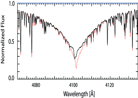
Figure 1: Synthesized H$\delta$ profile of the composite spectrum (gray, or red online). The observed spectrum (black) shows a partially filled in, and shifted core.

Because the strong profiles of the primary star were not well reproduced after broadening by a rotational profile, we added a gaussian macroturbulent velocity. The adopted values were $v\cdot\sin(i)$ of 8 $\rm km\,s^{-1}$  for the rotational velocity and $\xi_{M}=9$ $\rm km\,s^{-1}$  for the gaussian macroturbulent velocity.

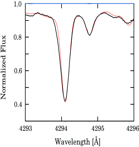
Figure 2: Comparison of the asymmetric observed profile at 4294.1 Å (black line) with the synthetic blend profile due to Ti II 4294.094 Å and Fe I 4294.125 Å (gray, red online).

While the weak and medium-strong profiles were well predicted by the combined velocity broadenings, the strong lines showed an asymmetric profile with a more extended violet wing that was impossible to reproduce with our computations. An example is shown in Figure 2. This kind of profile which could indicate an expanding atmosphere, is seen in many lines in both the UVES and HARPS spectra.

The microturbulent velocity value $\xi_{t}=2.5$ $\rm km\,s^{-1}$  for the primary star was determined both from the equivalent widths and the synthetic spectrum methods.

4.1.2 The secondary

The spectrum of HD 104237 is contaminated by that of the close companion. FB analyzed a spectrum that was obtained by subtracting a computed spectrum for the secondary from the observed spectrum.

We have preferred to analyze the observed spectrum as it is, and have tried to obtain information also from the secondary spectrum. This was not trivial, mostly because no usual spectroscopic methods for the parameter determinations can be applied to the close companion. In fact, neither hydrogen lines nor elements with lines in two different ionization stages are independently observable. We based our parameters for the secondary mostly on the Ca I line at 6122.21 Å which is a good luminosity indicator (Cayrel et al. 1996). The two components for this line are rather well separated and free of blends. Unfortunately, the other two lines of the Ca I triplet at 6102.73 Å and 6161.30 Å are blended.

The composite synthetic spectrum normalized to the continuum (PS) was computed according to the relation (Lyubimkov & Samedov, 1987)

$$\frac{F_{\lambda}(PS)}{F_{\lambda c}(PS)}=\frac{F_{\lambda}(P)R_{P}^{2}+F_{\lambda}(S)R_{S}^{2}}{F_{\lambda c}(P)R_{P}^{2}+F_{\lambda c}(S)R_{S}^{2}}.$$ (1)

We use the subscript ‘$\lambda c$’ to indicate the continuum $at$ a wavelength $\lambda$. The $F$’s for the primary (P) and secondary (S) have units of energy per unit area, per sec, per Ångström. The $R$’s, are the stellar radii.

After some experimentation with alternate models and different radii ratios, we selected a ratio $R_{S}/R_{P}=1$ (see Section 4.4), and the parameters $T_{\rm eff}$ = 4800 K and log(g) = 3.7 for the secondary. A rotational velocity v sin(i) = 12 km s^-1 was deduced from the comparison of the observed and computed profiles. We thank the referee, Barry Smalley, who pointed out that the same v sin(i) and macroturbulence (8 and 9 $\rm km\,s^{-1}$, respectively) would have nearly the same combined profile as a v sin(i) of 12 and no macroturbulence. This would be the case if the stars were tidally locked.

A microturbulent velocity $\xi_{t}$ = 1.0 km s^-1 and solar abundances were assumed. FB used $T_{\rm eff}$ = 4500K, log(g) = 4.0 and assumed solar abundances and a microturbulent velocity $\xi_{t}$ = 2 km s^-1.

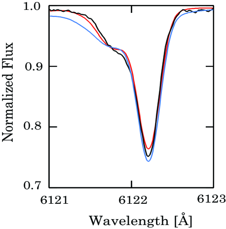
Figure 3: Observed (black) and calculated Ca i  $\lambda$6122.21, with $\log(g)=3.7$ (light gray/red online), and $\log(g)=4.0$ (dark gray/blue online). The main feature is due to the primary. Absorption from the same line in the secondary star (see text) is to the violet.

Figure 3 compares the observed Ca I profile at 6122.21 Å with the composite profiles computed for $T_{\rm eff}$ = 8250 K, and $\log(g)$ = 4.2 for the primary and for both $T_{\rm eff}$ = 4800 K, and $\log(g)$ = 3.7 and $T_{\rm eff}$ = 4500 K, and $\log(g)$ = 4.0 for the secondary. In the first case the ratio of radii is $R_{S}/R_{P}=1$, in the second case it was deduced from the relation

$$\frac{R^{2}_{S}}{R^{2}_{P}}=\frac{M_{S}}{M_{P}}\cdot\frac{g_{P}}{g_{S}}.$$ (2)

for a mass ratio M_P/M_S = 1.29 (Böhm et al. 2004). The too-broad wing of the secondary star profile computed for log($g$) = 4.0 is evident.

The adopted parameters for the two components (Table. 2) were well suited to reproduce several primary-secondary pairs of profiles as Fe i  at 4950.11, 4969.92, 5002.793, 5393.17, 5576.09 Å, 6065.48, 6252.56, 6335.33 Å, Ca i  6717.68 Å, and several others.

4.2 Equivalent widths

A closely related approach makes use of measurements in the observed composite spectrum (Figure 4). Voigt-profile fits are used to derive equivalent widths. These values are then related to computed equivalent widths from the adopted models, assuming solar abundances.

Equivalent widths were not used to derive atmospheric parameters or abundances for the secondary star, with the exception of lithium (Sec. 5.4).

Let $x_{\lambda}=L_{\lambda c}(S)/L_{\lambda c}(P)$ be the continuum luminosity ratios, where $L_{\lambda c}(S)=F_{\lambda c}(S)\cdot 4\pi R_{S}^{2}$, and similarly for the primary. With the parameters given in Table 2, the flux ratio $F_{\lambda c}(S)/F_{\lambda c}(P)$ at $\lambda$ = 5576 Å is $1/9.9$. Because of our assumption of equal stellar radii, the ratio is the same for the luminosities.

Directly measured equivalent widths from the composite spectrum must be corrected to account for the relative contribution of the light of the two stars. Assume that the flux in a line of the primary component is diluted only by the continuum flux of the secondary component. Then the equivalent width of a line of the P-component measured in the composite spectrum, $W_{P}^{PS}$, is related to the equivalent width, $W_{P}$ in the undiluted spectrum by

$$W_{P}=(1+x_{\lambda})\cdot W_{P}^{PS}$$ (3)

Using a similar notation, the (undiluted) equivalent width of the secondary component may be obtained from

$$W_{S}=\frac{1+x_{\lambda}}{x_{\lambda}}\cdot W^{PS}_{S}.$$ (4)

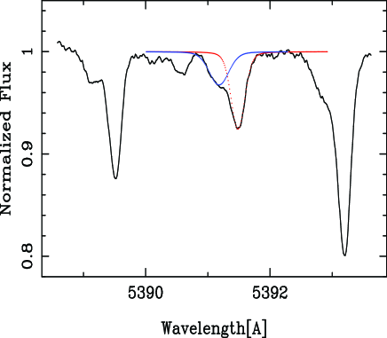
Figure 4: Fe i  $\lambda$5391.46, showing Voigt-profile fits to absorptions from components P and S (weaker, violet component). Lines from the secondary can also be seen in the stronger lines, Fe i, $\lambda\lambda$5389.49, and 5393.17

Figure 4 illustrates measurements on the composite UVESPOP spectrum. It can be seen that the assumption that the lines of the two components are separate from one another is only approximately true. This assumption is implicit in Eqs. 3 and  4. However, direct comparisons between equivalent width and results from complete synthesis (including the secondary), are in good agreement, showing that the approximation used here are good to a few hundredths of a dex. At longer wavelengths, the separation of the components is greater than that shown in Figure 4.

Equivalent widths of Fe i and Fe ii lines were measured, and corrected as indicated. This is basically an iterative procedure. The fraction $x_{\lambda}$ in Eqs. 3 and  4 follows from measurements of the diluted ($W_{P}^{PS}$, and $W_{S}^{PS}$) and $calculations$ of the undiluted ($W_{P}$ and $W_{S}$) equivalent widths. Calculations of the latter require models, but initial models are available from FB. Adopted models must give similar values of $x_{\lambda}$ from either Eq. 3 or  4.

If the flux ratios, $x_{\lambda}$, are known, equivalent widths of Fe i  and Fe ii  lines may be used along with a grid of atmospheres to determine a relation between $T_{\rm eff}$ and $\log(g)$.

We also examined line-by-line abundances for other atomic and ionic species with numerous lines, to check that the abundances did not drift with excitation potential. This provides an independent check on $T_{\rm eff}$

The overall procedure has the advantage that weak lines ($W_{\lambda}\approx$ 25 mÅ  or less) may be used. These are in principle, independent of line broadening mechanisms and the instrumental profile.

The synthesized spectra were useful for the selection of lines that were free from blends, and could be used for abundances in the equivalent width method. Indeed, the synthetic spectrum automatically includes relevant line absorption from the secondary when it overlaps with lines of the primary star. Contributions from the secondary are indicated automatically on the synthesized spectrum, making it straightforward to see when a feature is influenced by an accidental overlap with an absorption from the secondary star.

The adopted models made use of both spectrum synthesis and equivalent widths. Their parameters are given in Table 2. Uncertainty estimates for the primary are based on comparisons of results of calculations based on a grid of models with parameters surrounding the adopted values.

The comparison of the observed profiles of Ca I at 6122 A with profiles computed for several different choices of Teff and logg has lead us to select as best parameters $T_{\rm eff}$ 4800 K and log($g$) $\leq$3.7, with an uncertainty of 0.2 dex. While there is an uncertainty of about 200K for the temperature, the value of the gravity is an upper limit. In fact, values of log($g$)= 3.6 and 3.5 would have been as well suited to reproduce the observed profile for temperatures differing within $\pm$200K from 4800K.

AW used $T_{\rm eff}$ =  8000K, and $\log(g)=4.5$. FB’s values were 8550K, and $\log(g)=3.9$, for the primary.

Table 2: Adopted parameters for primary and secondary atmospheres

	$T_{\rm eff}$K	$\log(g)$	$\xi_{\rm turb}$
Primary	8250$\pm$200	4.2$\pm$0.25	2.5$\pm$1
Secondary	4800$\pm$200	$3.5-\leq 3.7$	1.0$\pm$1

4.3 Pulsational studies

Astroseismological measurements are being used to predict masses, radii, luminosity, and ages of stars (Mathur, et al. 2012). Dupret, et al. (2006) attempted to fit the pulsation frequencies discussed by Böhm, et al. (2004) to theoretical models. They found that the stellar properties that fit the observed frequencies were not in good agreement with best estimates of these values by other methods. Subsequently, Dupret et al. (2007) suggested He accumulation in the partial ionization zone to account for the observed modes.

While FB reported extensive pulsational observations and analysis, they chose classical spectroscopic methods to determine $T_{\rm eff}$ and $\log(g)$ for HD 104237. Those methods are basically the same as the ones used in the present work. We conclude that astroseismic constraints need to be complemented by spectroscopic analysis; pulsational properties alone are not yet sufficient, at least for HD 104237.

4.4 Radii, masses, and consistency

One approach to the ratio of the radii of the primary and secondary of the HD 104237 system is to use the ratio of absorption lines, such as those shown in Fig 4. We measured equivalent widths of five Fe i  lines $\lambda\lambda$ 6065.48, 6252.56, 6336.82, 6411.65 & 6421.35, to derive the factor $x_{\lambda}=0.155$ of Eqs.  3 and  4. Since that ratio is defined by

$$x_{\lambda}=\frac{L_{\lambda c}(S)}{L_{\lambda c}(P)}=\frac{R^{2}_{S}}{R^{2}_{P}}\cdot\frac{F_{\lambda c}(S)}{F_{\lambda c}(P)}$$ (5)

we may use the empirically determined $x_{\lambda}$ to obtain the ratio of the radii. Note the luminosities and fluxes are wavelength dependent. The models of Table 2 provide the surface fluxes for each of the stars. That ratio at 6310 Å is 0.139, for the surface flux of the secondary to that of the primary. With these numbers we obtain $R_{S}/R_{P}=1.06$, or unity within the uncertainties discussed in this section and given in Table 2.

Another way for finding the ratio of radii is the use of the Stefan-Boltzmann law. Here, we need the total luminosities (integrated over wavelength). Then

$$\frac{L(P)}{L(S)}=\frac{R^{2}_{P}}{R^{2}_{S}}\cdot\frac{T^{4}_{eff}(P)}{T^{4}_{eff}(S)}$$ (6)

Assuming a luminosity ratio of 10 (Böhm et al. 2004) the ratios of radii for T_eff(P) = 8250 K and T_eff(S) = 4800 K is R_P/R_S = 1.07.

Yet another approach to finding the ratio of the radii is to use the spectroscopically determined surface gravities and Eq. 2. Assuming a mass ratio $M_{P}/M_{S}$ of 1.29 (Böhm et al. 2004), $\log(g_{S})=3.7$, and $\log(g_{P})=4.2$, the ratio of radii R_P/R_S is 1.6. For R_P/R_S = 1, and the same gravities as before, we obtain $M_{P}/M_{S}$ = 3.15.

Therefore, while we found a rather good consistency between the ratios of radii, luminosities, and effective temperatures related by the Stefan-Boltzmann law, we obtain a manifest inconsistency between the ratios of radii, masses, and gravities related by the universal gravitation law. The mass ratio obtained by us is in conflict with the value of 1.29 of Böhm, et al. (2004). However, we must take the uncertainties into account.

We note that the spectroscopic gravity for both the primary and secondary stars are affected by errors which depend first of all on the position of the continuum, which is rather difficult to draw, in particular above the hydrogen lines. Furthermore, the parameters for the secondary are based on too many assumed or estimated quantities to allow quantitative analyses of the secondary unaffected by some large uncertainties.

Spectroscopic gravities typically have an uncertainty of 0.2 (or more) in the log. If we were to assume 4.0 and 3.9 for the surface gravities of the primary and secondary, then, still with unity for the ratio of the radii, we would obtain 1.26 for the mass ratio. These gravity changes would affect the derived abundances by only a few hundredths of a dex. Böhm, et al. (2004) assign an uncertainty of 0.02 to their mass ratio, so their value could be 1.27. While there is room for future adjustments of the fundamental parameters of this system, we conclude there is no significant conflict of our parameters with the spectroscopic mass ratio.

5 Abundances

5.1 Previous abundance work

In this section, we briefly compare and contrast our work with that of AW and FB. In the latter study, only the iron abundance was determined–independently from Fe i  and Fe ii.

Both AW and FB study derive abundances from equivalent widths. Although AW did not account for dilution by the secondary spectrum, their abundance results are similar to ours. For the well-represented iron spectra (Fe i  and  ii ) differences are under 0.1 dex. Differences are less than a factor of two, apart from Cu, and two trace species, Nd and Sm, where AW report rather large excesses of +0.59 and +0.85 dex. If we average the absolute value of the logarithmic differences, “This study minus AW”, the value is 0.13 dex for the elements through barium.

FB (see their Table 5) give $-$4.38 for log(A_Fe), or $\log(Fe/H)$. This becomes $-$4.42 for $\log(Fe/N_{tot})$. This differs from our value (Table 4) by only 0.02 dex.

Lines from the secondary and weak, previously unclassified lines could account for the large excesses of Nd and Sm reported by AW. An example is shown in Figure 5, where Fe I $\lambda$4061.09 coincides with Nd II $\lambda$4061.09. The upper level of the Fe I line in question was given by Nave, et al. (1994), but is not in Sugar and Corliss (1985).

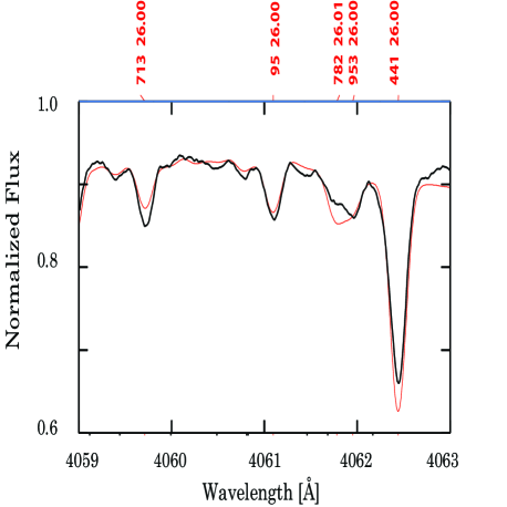
Figure 5: A previously unclassified Fe I line at $\lambda$4061.09 (34362.87–58979.82 cm^-1) very closely coincides with a strong line of Nd II. Synthesis shows the corresponding feature in HD 104237 is mostly Fe I. A minor contribution of a few mÅ, commensurate with a solar Nd abundance is likely. Labels at the top of the plot indicate lines from the primary (gray/red online). The decimal fraction of the wavelength is followed by the element (e.g. 26.01 is Fe ii). The standard SYNTHE plots also contain information on line strengths, and excitation.

FB used abundances from Fe i  and Fe ii  to fix $T_{\rm eff}$ and $\log(g)$. Both FB and AW used excitation to break the $T_{\rm eff}$-$\log(g)$  degeneracy. Neither work computed Balmer profiles.

With the help of estimates of the $T_{\rm eff}$ and $\log(g)$ of the secondary, FB synthesized its spectrum, and subtracted it from the observed composite. This method therefore differed from the present technique, in which a composite spectrum was synthesized and compared directly with the observed spectrum. We see no particular advantage or disadvantage of subtracting the secondary rather than synthesizing the composite spectrum. While FB took the secondary into account in their analysis of the primary, they do not report abundances for the secondary.

Given an accurate synthesis of the secondary, FB’s method assured their equivalent widths were unperturbed by blends from the secondary. In the our equivalent width method, such blends were avoided with the help of the results from the composite synthesis, where contributions from the primary and secondary spectrum are indicated on the plots (see Figure 5).

FB were careful to make use of lines with well-defined continua, and accurate oscillator strengths. These constraints, however, reduced the number of usable lines to 8 Fe i  lines and only 2 Fe ii  lines. Just 3 of these lines were below 30 mÅ. The remainder were subject to saturation corrections dependent on the microturbulence, $\xi_{t}$. This was not independently determined, but fixed at 2 $\rm km\,s^{-1}$, based on previous studies. AW used $\xi_{t}=3$ $\rm km\,s^{-1}$.

Table 3 illustrates the influence of the assumed microturbulence on abundance for two Fe i  lines, $\lambda$4736 (74 mÅ) and $\lambda$4485 (48 mÅ). The entries give the difference in logarithmic abundance from that obtained with $\xi_{t}=0.0$. We see that for the 74 mÅ  line, the abundance difference using 2.0 and 2.5 $\rm km\,s^{-1}$  is 0.82 $-$ 0.69 = 0.13 dex. For the weaker line, the difference is only 0.02 dex. For reference, note that in a recent study of Herbig AeBe stars, Folsom, et al. (2012) reported values of $\xi_{t}$ between 1.3 and 3.7 $\rm km\,s^{-1}$.

Table 3: The effect of microturbulence on abundance

$\xi_{t}$($\rm km\,s^{-1}$)	log(diff)
	4736(74mÅ)	4485(48mÅ)
0.0	0.00	0.00
1.0	0.26	0.04
2.0	0.69	0.09
2.5	0.82	0.11
3.0	0.91	0.13
3.5	0.98	0.14

We determined $\xi_{t}$ independently for each spectrum, obtaining values ranging up to 3.3 $\rm km\,s^{-1}$. Eventually we adopted 2.5 $\rm km\,s^{-1}$, which was more compatible with the spectrum synthesis fits. However, our abundances based on equivalent widths of weak lines are virtually independent of this choice.

5.2 Present results

Equivalent widths, oscillator strengths, and abundances are available in the online material for some 375 absorption lines. Abundances were obtained from these equivalent widths using the Michigan software, usually for for the weak lines and are in consistent agreement with best fits from detailed spectrum synthesis.

Abundances are summarized in Table 4. Some spectra, e.g. Ca ii, were not used for abundances, even though their lines were clearly present. This was usually because of blends and/or oscillator strengths with low accuracy. Such cases are indicated by “n.u.” (not used), in the table. Probable errors (pe) are standard deviations of abundances from the number of lines given in the column labeled ‘$n$’. For $n=2$, the error is the difference of abundances. For an element, e.g. Fe (Fe i  and Fe ii), the error is the difference of values from the atomic and ionic spectra. The column marked ‘AW’ gives logarithmic abundances computed from AW’s paper. We used the Anders & Grevesse (1998) solar abundances to compute $\log(El/N_{tot})$ from the bracket values given by AW. One exception is Fe, where AW used 7.52 (log(H) = 12) rather than 7.67 given by Anders and Grevesse for the photospheric iron abundance. The solar abundances in Column 7 are from Asplund, et al.(2009).

Table 4: Adopted abundances. Column 2 is a key to oscillator-strength references given in the appendix. See text for a description of the column labeled AW.

Spec	$gf$-ref	$\log(El/N_{\rm tot})$	pe	n	AW	Sun
Li i	1	Table 5
C i	2	$-$3.64	0.12	8	$-$3.62	$-$3.61
N i	3	$-$4.13	0.07	4	$-$4.41	$-$4.21
O i	4	$-$3.31	0.09	5	$-$3.21	$-$3.35
Na i	5	$-$5.64	0.01	2	$-$5.64	$-$5.80
Mg i	6	$-$4.79	0.30	5	$-$4.58	$-$4.44
Mg ii	7	n.u.			$-$4.65
Al i	8	$-$5.66	0.30	4	$-$5.59	$-$5.59
Si i	9	$-$4.51	0.44	7	$-$4.47	$-$4.52
Si ii	10	n.u.			$-$4.18
S i	11	$-$4.70	0.02	2	$-$4.98	$-$4.92
Ca i	12	$-$5.79	0.08	4	$-$5.53	$-$5.70
Ca ii	13	n.u.			$-$5.54
Sc ii	14	$-$8.63	0.20	5	$-$8.87	$-$8.98
Ti i	15	$-$7.05	0.11	3
Ti ii	16	$-$7.12	0.16	5	$-$6.82
Ti		$-$7.08	0.07			$-$7.09
V i	17	$-$8.06	0.15	1
V ii	18	$-$7.77	0.21	3
V		$-$7.97	0.29		$-$8.05	$-$8.11
Cr i	19	$-$6.31	0.25	7
Cr ii	20	$-$6.26	0.13	7	$-$6.20
Cr		$-$6.29	0.05			$-$6.40
Mn i	21	$-$6.63	0.17	4	$-$6.70	$-$6.61
Mn ii	22	n.u.
Fe i	23	$-$4.37	0.13	22	$-$4.44
Fe ii	24	$-$4.42	0.17	17	$-$4.42
Fe		$-$4.40	0.05			$-$4.54
Co i	25	$-$7.26	0.08	2		$-$7.05
Ni i	26	$-$5.70	0.19	10	$-$5.70	$-$5.82
Ni ii	27	n.u.		2
Cu i	28	$-$7.96	0.25	3	$-$7.57	$-$7.84
Zn i	29	$-$7.58	0.25	2	$-$7.81	$-$7.48
Sr ii	30	$-$9.17:	0.30:	2		$-$9.17
Y ii	31	$-$9.69	0.13	4	$-$9.62	$-$9.83
Zr ii	32	$-$9.06	0.06	4	$-$9.09	$-$9.46
Ba ii	33	$-$9.61	0.20	5	$-$9.60	$-$9.86
La ii	34	$-$10.72	0.10	3	$-$10.72	$-$10.94

Most elements are solar within the errors. We examined features near lines of the light lanthanides, Ce-Sm, but they were weak and often blended with absorption from the secondary. We see no indication these elements are significantly different from solar in abundance.

A case could be made for slight enhancements of a few elements. The case for Zr is the strongest. There are numerous lines, modern gf-values (Ljung, et al. 2006) and the abundance excess is several times the uncertainty. The lithium abundance is discussed below.

5.3 The secondary

In addition to Li I, we identified in the secondary lines of Na I, Mg I, Al I, Si I, Ca I, Sc I, Ti I, V I, Cr I, Mn I, Fe I, Co I, Ni I, Cu I, Zn I, Sr I, Ba II. A large number of molecular lines, especially of C2, CN, CO, CH, MgH contribute to lower the continuum. We found several underabundances. Logarithmically, relative to solar, they were for Sc [$-$0.3], Ti [$-$0.4], V [$-$0.4], Cr [$-$0.4], Co [$-$0.7], Ni [$-$0.3]. Furthermore, in addition to Li, we found an overabundance for Ba [+0.5]. All the other elements are well predicted by solar abundances. We note that these abundances are estimates derived from the comparison of the observed UVESPOP spectrum with the synthetic spectrum. More work would be needed for an accurate quantitative analysis of the companion of HD 104237.

5.4 Lithium

While lithium is commonly observed in young, cool stars, we are unaware of its observation in other Herbig Ae stars. Of course, a strong Li i  line was noted in HD 104237 by FB and others, and correctly attributed to the cooler secondary. Böhm, et al. (2004) discuss the lithium line in both primary and secondary, but we know of no prior abundance determinations from either line in HD 104237.

Lithium is the only light element that shows a clear departure from the solar photospheric abundance. The Li i  region is shown in Figure 6. The weaker feature marked by a vertical line, is Li i  in the primary. Note the stronger feature, Li i  in the secondary, is to the red in HARPS(b).

An abundance is derived for both primary and secondary spectra from equivalent widths as well as synthesis. Only abundances from the HARPS(b) spectrum (Figure 6, below), where the primary and secondary lines are well separated, are adopted. Note that when we apply the correction of Eq. 4 to the equivalent width for the secondary, 38.1 mÅ, using $x_{\lambda}$ = 0.171, we get 261 mÅ, a line no longer weak. The abundance, $\log(Li/N_{tot})=-9.28$ was calculated with the full hfs structure (cf. Smith, Lambert & Nisson 1998). A solar mix of ⁶Li and ⁷Li was assumed.

To estimate errors in the lithium abundances, we use HARPS(b) values. Comparing abundance results from from synthesis and equivalent widths, we estimate the uncertainties for the lithium abundances are about 0.1 dex for the primary and 0.25 dex for the secondary.

The lithium abundance for the primary may be slightly enhanced with respect to the meteoritic value (Lodders, Palme & Gail 2009). There is evidence for some destruction of lithium in the cooler secondary.

Table 5: Lithium abundances from $\lambda$6707. See text for uncertainty estimates.

Primary		Secondary
$W_{\lambda}$/Rem	$\rm\log(Li/N_{tot})$	$W_{\lambda}$	$\rm\log(Li/N_{tot})$
13.6/HARPS(b)	$-$8.58	38.1	$-$9.28
synthesis:
uves	$-$8.64		$-$8.90
HARPS(a)	$-$8.64		$-$8.90
HARPs(b)	$-$8.64		$-$9.50
(solar photosphere:)	$-$10.99
(meteorite:)	$-$8.79

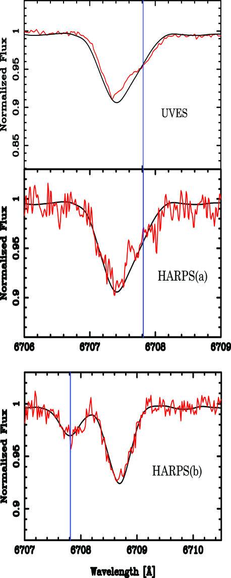
Figure 6: The Li i  region, showing synthetic fits. See Section  2 for epochs of the UVES, HARPS(a) and HARPS(b) spectra (gray, red online). The vertical line marks the rest wavelength of Li I in the primary. Abundances in Table 5 were used for the lower plot. Note the different wavelength scales for the upper two, and the lower plots.

6 The emission-line spectrum

In this section we compare and contrast the emission-line spectra of HD 104237 with two sharp-lined Herbig Ae stars HD 101412 and HD 190073. Spectra and abundances for these stars were discussed by Cowley, et al. (2010), and Cowley & Hubrig (2012). Emission lines increase in prominence from HD 101412 to HD 104237 and finally to HD 190073. Properties of the more prominent emission lines in these three spectra are given in Table 6. The maximum intensity, or $I$-value, and equivalent width, $W$ are with respect to the continuum; emission below the continuum line is not taken into account.

Table 6: Properties of selected emission lines

			FWHM
Star(HD)/line	Max $I$	W[Å]	[Å]	$\rm km\,s^{-1}$
H$\alpha$
101412	3.39	10.5	4.42	202
104237	3.55	13.3	4.71	215
190073	6.82	32.2	5.34	244
Na D2
101412	1.11	0.26	2.36	120
104237	1.45	1.03	1.97	100
190073	1.76	1.38	1.38	70
Fe ii 5169
104237	1.37	1.04	2.17	126
190073	1.77	1.89	2.14	124
Mg i(b1) 5184
104237	1.06	0.10	1.48	86
190073	1.45	1.03	1.97	114
$[\rm O]$ i  6300
101412	1.07	0.125	1.71	81
104237	1.04	0.017	0.75	36
190073	1.11	0.056	0.41	20

Only a few emission lines are seen in HD 101412. These include the low Balmer members, the sodium D-lines, and He i  (D₃ or $\lambda$5876), which is weakly in emission. The strong Fe ii  Multiplet 42, so often in emission in young stars is in absorption. Indeed, it is somewhat more strongly in absorption than would be expected from the other Fe ii  lines, as described by Gray and Corbally (2009, see their Nab class). Neither the Ca ii  H and K lines nor the infrared triplet is in emission.

Both HD 104237 and HD 190073 show the typical emission lines of young stars, including the Balmer, Ca ii  and numerous lines from the first but mostly second spectra of iron-group elements.

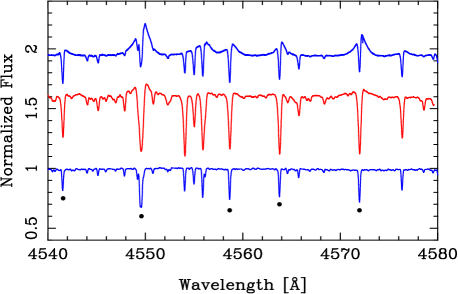
Figure 7: Emission and absorption lines in HD 104237 (center), HD 101412 (lower), and HD 190073 (upper). Lines marked with filled circles are discussed in the text.

Figure 7 illustrates some of the weaker emission lines in these stars. The strongest lines in this region are dominated by Ti ii, $\lambda$4549.60 and 4571.97. Weaker emissions, Fe ii $\lambda$4541.56, Cr ii  $\lambda$4558.65, and Ti ii  $\lambda$4563.76 are stronger in HD 190073 than in HD 104237. No emissions are evident in HD 101412.

7 Discussion

Herbig AeBe stars have been investigated as possible progenitors of magnetic Ap/CP stars (Drouine et al. 2004, Folsom, et al. 2012). A modest fraction of these stars are magnetic (ca. 5-10% Hubrig, et al. 2010, Alecian, et al. 2012), as is the case with their main-sequence congeners (Power, et al. 2008). The chemistry of the Herbig stars is less indicative of an evolutionary connection. A few of the Herbigs do indeed have abundance excesses that could connect them to classical, magnetic Ap stars (Vick, et al. 2011). However, the most common peculiarity that has emerged so far, is a resemblance to the $\lambda$ Boo stars.

In their new detailed study, Folsom, et al. (2012) concluded that about half of their sample of 20 stars showed $\lambda$ Boo characteristics. We had made independent abundance studies of two of the Folsom et al. stars, HD 101412 (Cowley, et al. 2010), and HD 190073 (Cowley & Hubrig 2012). The Folsom et al. results for these stars are in excellent agreement with ours. These two stars as well as HD 104237 have relatively sharp spectral lines, an important feature for accurate analysis. One star, HD 101412, has mild $\lambda$ Boo abundances, while two, HD 190073 and HD 104237 (present paper) have solar abundances (apart from Li). Indeed, the connection between young stars and the $\lambda$ Boo type has recognized for some time (Gray & Corbally 1998).

The prominence of $\lambda$ Boo types among the Herbig AeBe complicates the theoretical understanding of these stars. The received mechanism for Ap/CP chemistry, diffusion (Michaud 1970), is quite different from that commonly discussed for the $\lambda$ Boo stars, gas-grain separation (cf. discussion and references in AW).

HD 104237 has mostly solar abundances, as noted by AW. Its excess of lithium is expected for a young star. The largest departure from solar reported here is for zirconium, whose excess in field stars is usually associated with the s-process. If there is an indication of the s-process among related elements (Sr, Y, Ba, La), it is marginal.

8 Acknowledgements

We thank J. R. Fuhr J. Reader, and W. Wiese of NIST for advice on atomic data and processes, M. Briquet for help with the section on pulsations, and J. F. González for help with the observational material. We are grateful S. Bagnulo and the UVESPOP team for their valuable archive. This research has made use of the SIMBAD database, operated at CDS, Strasbourg, France. Our calculations have made extensive use of the VALD atomic data base (Kupka, et al. 1999), as well as the NIST online Atomic Spectroscopy Data Center (Kramida, et al. 2013). CRC is grateful for advice and helpful conversations with many of his Michigan colleagues. We thank the referee, B. Smalley, for valuable comments and suggestions which have strengthened this contribution.

REFERENCES

Acke, B., Waelkens, C. 2004, A&A, 427, 1009 (AW)

Aldenius, M., Lundberg, H., Blackwell-Whitehead, R. 2009, A&A, 502, 989

Alecian, E., Wade. G. A., Catala, C., Grunhut, J. H., Landstreet, J. D., Bagnulo, S., et al. 2013, MNRAS, 429, 1001

Anders, E. & Grevesse, N. 1989, Geochim. Cosmochim. Acta, 53, 197

Asplund, M., Grevesse, N., Sauval, A. J., Scott, P. 2009, Ann. Rev. Astron. Ap. 47, 481

Bagnulo, S. Jehin, E., Ledoux, C., Cabanac, R., Mello, R., Gilmozzi, R., et al. 2003, The Messenger, 114, 10

Böhm, T., Catala, C., Balona, L. & Carter, B. 2004, A&A, 427, 907

Biémont, É., Blagoev, K., Engstrom, L. et al. 2011, MNRAS, 414, 3350

Blackwell, D. E., Menon, S. L. R., Petford, A. D. & Shallis, M. J. 1982, MNRAS, 201, 611

Castelli, F. 2010, wwwuser.oat.ts.astro.it/castelli/grids.html

Castelli, F. & Hubrig, S. 2004, A&A, 425, 263

Castelli, F. & Kurucz, R. L. 2003, in Modelling of Stellar Atmospheres, ed. N. Piskunov, W. W. Weiss, D. F. Gray, IAU Symposium 210, p. 424

Cayrel, R., Faurobert-Scholl, M., Feautrier, N., Spielfield, A. & Thevenin, F. 1996, A&A, 312, 549

Cowley, C. R., Adelman, S. J. & Bord, D. J. 2003, in Modelling of Stellar Atmospheres, IAU Symp. 210, ed. N. Piskunov, W. W. Weiss & D. F. Gray, p. 261

Cowley, C. R. & Hubrig, S. 2012, AN, 333, 34

Cowley, C. R., Hubrig, S., González & Savanov, I. 2010, A&A, 523, 65

Davidson, M. D., Snoek, L. C., Volten, H. & Dönszelmann, A. 1992, A&A, 255, 457

den Hartog, E. A., Lawler, J. E., Sobeck, J. S., Sneden, C. & Cowan, J. J. 2011, ApJS, 194, 35

Donati, J.-F., Semel, M., Carter, B. D., Rees, D. E. & Collier Cameron, A. 1997, MNRAS, 291, 658.

Dupret, M.-A, Böhm, T., Goupil, M.-J., Catala, C., Grigahcène, A. 2006, Comm. Astroseismology, 147, 72

Dupret, M.-A., Théado, T, Böhm, T., Goupil, M.-J., Catala, C., Grigahcène, A. 2007, Comm. Astroseismology, 150, 59

Drouine, D., Wade, G. A., Bagnulo, S., Landstreet, J. D., Mason, E. & Monin, D. N. 2004, in The A-Star Puzzle, IAU Symp. 224, 506.

Feigelson, E. D., Lawson, W. A. & Garmire, G. P. 2003, ApJ, 599, 1207

Fisher, C. F. 2002, private (cf. NIST site for Mg II)

Folsom, C. P., Bagnulo, S., Wade, G. A., Alecian, E., Landstreet, J. D., Marsden, S. C. & Wate, I. A. 2012, MNRAS, 422, 2072

Fuhr, J. R. & Wiese, W. L. 2005, in CRC Handbook of Chem. & Physics, 86th ed. 10-93 (ed. D. R. Lide, CRC Press, Boca Raton, FL)

Fuhr, J. R. & Wiese, W. L. 2006, J. Phys. Chem. Ref. Data, 35, 1669

Fumel, A. & Böhm, T. 2012, A&A, 540, 108 (FB)

Grady, C. A., Woodgate, B., Torres, C. A. O., Henning, Th, Apai, D., Rodmann, J., et al. 2004, ApJ, 608, 809

Gray, R. O., & Corbally, C. J. 1998, AJ, 116, 2530

Gray, R. O. & Corbally, C. J. 2009, Stellar Spectral Classification (Princeton: Series in Astrophys.), see p. 203

Hibbert, A., Biémont, É, Godefroid, M. & Vaeck, N. 1993, A&AS, 99, 179

Hubrig, S., Pogodin, M. A., Yudin, R. V., Schöller, M. & Schnerr, R. S. 2007, A&A, 463, 1039

Hubrig, S., Schöller, M., Savanov, I., González, J. F., Cowley, C. R., Schütz, O., et al. 2010, AN, 331, 361

Hubrig, S., Stelzer, B., Schöller, M., Grady, C., Schütz, Pogodin, M. A., et al. 2009, A&A, 502, 283

Kelleher, D. E. & Podobedova, L. I. 2008, J. Phys. Chem. Ref. Data, 37, 267

Kupka, F., Piskunov, N. E., Ryabchikova, T. A., Stempels, H. C., Weiss, W. W. 1999, A&AS, 138, 119

Kramida, A., Ralchenko, Yu., Reader, J., and NIST ASD Team (2012). NIST Atomic Spectra Database (ver. 5.0), [Online]. Available: http://physics.nist.gov/asd [2013, February 21]. National Institute of Standards and Technology, Gaithersburg, MD.

Kurucz, R. L. 2005, MSAIS, 8, 14

Kurucz, R. L. 2012, http://kurucz.harvard.edu/atoms/

Lawler, J. E., Bonvallet, G. & Sneden, C. 2001, ApJ, 556, 452

Lawler, J. E. & Dakin, J. T. 1989, JOSA, 6B, 1457

Ljung, G., Nilsson, H., Asplund, M., Johansson, S. 2006, A&A, 456, 1181

Lodders, K., Palme, H. & Gail, H-P. 2009. Landolt-Börnstein, New Series, Astron. Astrophys. (arXiv:-901.1149).

Lyubimkov, L. S. & Samedov, Z. A. 1987, BCrAO 77, 109

Mayor, M., Pepe, F., Queloz, D., et al. 2003, Msngr, 114, 20.

Mathur, S., Metcalfe, T. S., Woitaszek, M., Bruntt, H., Verner, G. A., Christensen-Dalsgaard, J., et al. 2012, ApJ, 749, 152

Meléndez, J., Barbuy, B. 2009, A&A, 497, 611

Mendoza, C., Eissner, W., Le Dourneuf, M. & Zeippen, C. J. 1995, J. Phys. B28, 3485

Michaud, G. 1970, ApJ, 160, 641

Nahar, S. N. & Pradhan, A. K. 1993, J. Phys. B26, 1109

Nave, G., Johansson, S., Learner, R. C. M, Thorne, A. P. & Brault, J. W. 1994, ApJS, 94, 221

Nilsson, H., Ljung, G., Lundberg, H., Nielson, K. E. 2006, A&A, 445, 1165

Nitz, D. E., Kunau, A. E., Wilson, K. L. & Lentz, L. R. 1999, ApJS, 122, 557

NIST 2012, http://www.nist.gov/pml/div684/grp01/data.cfm

Ostrovskii, Yu. I. & Penkin, N. P. 1958, Opt. Spektrosk., 5, 345

Pickering, J. C., Thorne, A. P., Perez, R. 2001, ApJS, 132, 403 (Erratum: ApJS, 138, 247, 2002)

Pirronello, V. & Strazzulla, G. 1981, A&A, 93, 411

Power, J., Wade, G. A., Aurière, M, Silvester, J. & Hanes, D. 2008, Contrib. Astron. Obs. Skal. Pleso, 38, 443

Ryabchikova T.A., Piskunov N.E., Kupka F., Weiss W.W., 1997, Baltic Astron., 6, 244

Smith, V., Lambert, D. L. & Nissen, P. E. 1998, ApJ, 506,405

Sobeck, J.S., Lawler, J. E., Sneden, C. 2007, ApJ, 667, 1267

Sugar, J. & Corliss, C. H. 1985, J. Phys. Chem. Ref. Data, 14, Suppl. 2

Tachiev, G. I. & Fisher, C. F. 2002, A&A, 385, 716.

Vick, M., Michaud, G., Richer, J. & Richard, O. 2011, A&A, 526, 37

Wade, G. A., Bagnulo, S., Drouin, D., Landstreet, J. D. & Monin, D. 2007, MNRAS, 376, 1145

Wickliffe, M. E. & Lawler, J. E. 1997, ApJS, 110, 163

Yan, Z.-C & Drake, G. W. F. 1995, Phys. Rev. 52A, 4316

Appendix A Oscillator strength sources

Keys to oscillator strengths used for the individual spectra are given in column 2 of Table 4. A short indication is given here to complete citation found in the references. Compilations of NIST (Kramida et al. 2013), VALD (Kupka, et al. 1999), and Kurucz (2012) were used for lines not listed in modern primary sources.

Table 7: Short References for Table 4

Key	Short Ref.
(1)	Yan & Drake (1995)
(2)	Hibbert, et al. (1993)
(3)	Tachiev & Fisher (2002)
(4)	NIST/Kramida et al. (2013)
(5)	NIST/Kramida et al. (2013)
(6)	Kelleher & Podobedova (2008)
(7)	NIST/ Fisher, C. F. (2002)
(8)	Mendoza et al. (1995)
(9)	Nahar & Pradhan (1993)
(10)	Kurucz (2012)
(11)	VALD Ryabchikova, et al. (1997)
(12)	NIST & Aldenius, et al. (2009)
(13)	Kurucz (2012)
(14)	Lawler & Dakin (1989)
(15)	Blackwell, et al. (1982)
(16)	Pickering, et al. (2001)
(17)	NIST/Ostrovskii & (1958)
(18)	NIST & Kurucz (2012)
(19)	Sobeck, et al. (2007)
(20)	Nilsson, et al. (2006),VALD LS-permitted
(21)	VALD/den Hartog et al. (2011)
(22)	VALD/LS-permitted
(23)	Fuhr&Wiese (2006)
(24)	Meléndez&Barbuy (2009)
(25)	Nitz, et al. (1999)
(26)	VALD, Wicliffe&Lawler(1997)
(27)	VALD, LS-allowed
(28)	NIST/Fuhr & Wiese (2005)
(29)	VALD/Kurucz (2012)
(30)	Pirronello & Strazzula (1981)
(31)	Biémont, et al. (2011)
(32)	Ljung, et al. (2006)
(33)	NIST/Davidson, et al. (1992)
(34)	Lawler, et al. (2001)

Appendix B Online material

Equivalent widths, excitation potentials, oscillator strengths, and calculated abundances are available for individual lines as online material.

Table 8: Sample online material for C i. Weak lines used for the adopted abundances are marked with an asterisk

Wavelength EW   Log(EW)  loggf   Chi(eV) Log(C/Ntot)
4022.844   9.1    0.96  -2.650   7.480   -3.71*
4734.256  15.8    1.20  -2.370   7.950   -3.44*
4770.026  24.7    1.39  -2.440   7.480   -3.46*
4932.049  52.2    1.72  -1.660   7.680   -3.69
5052.167  93.4    1.97  -1.300   7.680   -3.61
6010.675   9.0    0.96  -1.940   8.640   -3.66*
7093.234  10.7    1.03  -1.700   8.650   -3.78*
7100.123  24.0    1.38  -1.470   8.640   -3.63*
7108.930  15.6    1.19  -1.590   8.640   -3.72*
7483.449  21.5    1.33  -1.370   8.770   -3.68*
7860.877  29.2    1.47  -1.150   8.850   -3.67