The linear stochastic order and directed inference for multivariate ordered distributions

Abstract

Researchers are often interested in drawing inferences regarding the order between two experimental groups on the basis of multivariate response data. Since standard multivariate methods are designed for two-sided alternatives, they may not be ideal for testing for order between two groups. In this article we introduce the notion of the linear stochastic order and investigate its properties. Statistical theory and methodology are developed to both estimate the direction which best separates two arbitrary ordered distributions and to test for order between the two groups. The new methodology generalizes Roy’s classical largest root test to the nonparametric setting and is applicable to random vectors with discrete and/or continuous components. The proposed methodology is illustrated using data obtained from a 90-day pre-chronic rodent cancer bioassay study conducted by the National Toxicology Program (NTP).

and

t1Supported in part by the Israeli Science Foundation Grant No 875/09.

t2Supported in part by the Intramural Research Program of the NIH, National Institute of Environmental Health Sciences (Z01 ES101744-04).

1 Introduction

In a variety of applications researchers are interested in comparing two treatment groups on the basis of several, potentially dependent outcomes. For example, to evaluate if a chemical is a neuro-toxicant, toxicologists compare a treated group of animals with an untreated control group in terms of various correlated outcomes such as tail-pinch response, click response and gait score, etc.; cf. Moser (2000). The statistical problem of interest is to compare the multivariate distributions of the outcomes in the control and treatment groups. Moreover, the outcome distributions are expected to be ordered in some sense. The theory of stochastic order relations [Shaked and Shanthikumar (2007)] provides the theoretical foundation for such comparisons.

To fix ideas let $\mathbf{X}$ and $\mathbf{Y}$ be $p$-dimensional random variables (RVs); $\mathbf{X}$ is said to be smaller than $\mathbf{Y}$ in the multivariate stochastic order, denoted $\mathbf{X}\preceq_{\mathrm{st}}\mathbf{Y}$, provided $\mathbb{P}(\mathbf{X}\in U)\leq\mathbb{P}(\mathbf{Y}\in U)$ for all upper sets $U\in\mathbb{R}^{p}$ [Shaked and Shanthikumar (2007)]. If for some upper set the above inequality is sharp, we say that $\mathbf{X}$ is strictly smaller than $\mathbf{Y}$ (in the multivariate stochastic order) which we denote by $\mathbf{X}\prec_{\mathrm{st}}\mathbf{Y}$. Recall that a set $U\in\mathbb{R}^{p}$ is called an upper set if $\mathbf{u}\in U$ implies that $\mathbf{v}\in U$ whenever $\mathbf{u}\leq$ $\mathbf{v}$, that is, if $u_{i}\leq v_{i}$, $i=1,\ldots,p$. Note that comparing $\mathbf{X}$ and $\mathbf{Y}$ with respect to the multivariate stochastic order requires comparing their distributions over all upper sets in $\mathbb{R}^{p}$. This turns out to be a very high-dimensional problem. For example, if $\mathbf{X}$ and $\mathbf{Y}$ are multivariate binary RVs, then $\mathbf{X}\preceq_{\mathrm{st}}\mathbf{Y}$ provided $\sum_{\mathbf{t}\in U}p_{\mathbf{X}}(\mathbf{t})\leq\sum_{\mathbf{t}\in U}p_{\mathbf{Y}}(\mathbf{t})$ where $p_{\mathbf{X}}(\mathbf{t})$ and $p_{\mathbf{Y}}(\mathbf{t})$ are the corresponding probability mass functions. Here $U\in\mathcal{U}_{p}$ where $\mathcal{U}_{p}$ is the family of upper sets defined on the support of a $p$-dimensional multivariate binary RV. It turns out that the cardinality of $\mathcal{U}_{p}$, denoted by $N_{p}$, grows super-exponentially with $p$. In fact $N_{1}=1$, $N_{2}=4$, $N_{3}=18$, $N_{4}=166$, $N_{5}=7579$ and $N_{6}=7\mbox{,}828\mbox{,}352$. The values of $N_{7}$ and $N_{8}$ are also known, but $N_{9}$ is not. However, good approximations for $N_{p}$ are available for all $p$; cf. Davidov and Peddada (2011). Obviously the number of upper sets for general multivariate RVs is much larger. Since in many applications $p$ is large, it would seem that the analysis of high-dimensional stochastically ordered data is practically hopeless. As a consequence, the methodology for analyzing multivariate ordered data is underdeveloped. It is worth mentioning that Sampson and Whitaker (1989) as well as Lucas and Wright (1991) studied stochastically ordered bivariate multinomial distributions. They noted the difficulty of extending their methodology to high-dimensional data due to the large number of constraints that need to be imposed. Recently Davidov and Peddada (2011) proposed a framework for testing for order among $K$, $p$-dimensional, ordered multivariate binary distributions.

In this paper we address the dimensionality problem by considering an easy to understand stochastic order which we refer to as the linear stochastic order.

Definition 1.1.

The RV $\mathbf{X}$ is said to be smaller than the RV $\mathbf{Y}$ in the (multivariate) linear stochastic order, denoted $\mathbf{X}\preceq_{l\mbox{-}\mathrm{st}}\mathbf{Y}$, if for all $\mathbf{s}\in$ $\mathbb{R}_{+}^{p}=\{\mathbf{s}\dvtx\mathbf{s}\geq 0\},$

$$\mathbf{s}^{T}\mathbf{X}\preceq_{\mathrm{st}}\mathbf{s}^{T}\mathbf{Y},$$ (1)

where $\preceq_{\mathrm{st}}$ in (1) denotes the usual (univariate) stochastic order.

Note that it is enough to limit (1) to all nonnegative real vectors satisfying $\|\mathbf{s}\|=1$, and accordingly we denote by $\mathcal{S}_{+}^{p-1}$ the positive part of the unit sphere in $\mathbb{R}^{p}$. We call each $\mathbf{s}\in\mathcal{S}_{+}^{p-1}$ a “direction.” In other words the RVs $\mathbf{X}$ and $\mathbf{Y}$ are ordered by the linear stochastic order if every nonnegative linear combination of their components is ordered by the usual (univariate) stochastic order. Thus instead of considering all upper sets in $\mathbb{R}^{p}$ we need for each $\mathbf{s}\in\mathcal{S}_{+}^{p-1}$ to consider only upper sets in $\mathbb{R}$. This is a substantial reduction in dimensionality. In fact we will show that only one value of $\mathbf{s}$ need be considered. Note that the linear stochastic order, like the multivariate stochastic order, is a generalization of the usual univariate stochastic order to multivariate data. Both of these orders indicate, in different ways, that one random vector is more likely than another to take on large values. In this paper we develop the statistical theory and methodology for estimation and testing for linearly ordered multivariate distributions. For completeness we note that weaker notions of the linear stochastic order are discussed by Hu, Homem-de Mello and Mehrotra (2011) and applied to various optimization problems in queuing and finance.

Comparing linear combinations has a long history in statistics. For example, in Phase I clinical trials it is common to compare dose groups using an overall measure of toxicity. Typically, this quantity is an ad hoc weighted average of individual toxicities where the weights are often known as “severity weights;” cf. Bekele and Thall (2004) and Ivanova and Murphy (2009). This strategy of dimension reduction is not new in the statistical literature and has been used in classical multivariate analysis when comparing two or more multivariate normal populations. For example, using the union-intersection principle, the comparison of multivariate normal populations can be reduced to the comparison of all possible linear combinations of their mean vectors. This approach is the basis of Roy’s classical largest root test [Roy (1953), Johnson and Wichern (1998)]. Our proposed test may be viewed as nonparametric generalization of the classical normal theory method described above with the exception that we limit consideration only to nonnegative linear combinations (rather than all possible linear combinations) since our main focus is to make comparisons in terms of stochastic order. We emphasize that the linear stochastic order will allow us to address the much broader problem of directional ordering for multivariate ordered data, that is, to find the direction which best separates two ordered distributions. Based on our survey of the literature, we are not aware of any methodology that addresses the problems investigated here.

This paper is organized in the following way. In Section 2 some probabilistic properties of the linear stochastic order are explored, and its relationships with other multivariate stochastic orders are clarified. In Section 3 we provide the background and motivation for directional inference under the linear stochastic order and develop estimation and testing procedure for independent as well as paired samples. In particular the estimator of the best separating direction is presented and its large sampling properties derived. We note that the problem of estimating the best separating direction is a nonsmooth optimization problem. The limiting distribution of the best separating direction is derived in a variety of settings. Tests for the linear stochastic order based on the best separating direction are also developed. One advantage of our approach is that it avoids the estimation of multivariate distributions subject to order restrictions. Simulation results, presented in Section 4, reveal that for large sample sizes the proposed estimator has negligible bias and mean squared error (MSE). The bias and MSE seem to depend on the true value of the best separating direction, the dependence structure and the dimension of the problem. Furthermore, the proposed test honors the nominal type I error rate and has sufficient power. In Section 5 we illustrate the methodology using data obtained from the National Toxicology Program (NTP). Concluding remarks and some open research problems are provided in Section 6. For convenience all proofs are provided in the Appendix where additional concepts are defined when needed.

2 Some properties of the linear stochastic order

We start by clarifying the relationship between the linear stochastic order and the multivariate stochastic order. First note that $\mathbf{X}\preceq_{l\mbox{-}\mathrm{st}}\mathbf{Y}$ if and only if $\mathbb{P}(\mathbf{s}^{T}\mathbf{X}\geq t)\leq\mathbb{P}(\mathbf{s}^{T}\mathbf{Y}\geq t)$ for all $(t,\mathbf{s})\in\mathbb{R}\times\mathbb{R}_{+}^{p}$ which is equivalent to $\mathbb{P}(\mathbf{X}\in H)\leq\mathbb{P}(\mathbf{Y}\in H)$ for all $H\in\mathcal{H}$ where $\mathcal{H}$ is the collection of all upper half-planes, that is, sets which are both half planes and upper sets. Thus $\mathbf{X}\preceq_{\mathrm{st}}\mathbf{Y}$ $\Rightarrow$ $\mathbf{X}\preceq_{l\mbox{-}\mathrm{st}}\mathbf{Y}$. The converse does not hold in general.

Example 2.1.

Let $\mathbf{X}$ and $\mathbf{Y}$ be bivariate RVs such that $\mathbb{P}(\mathbf{X}=(1,1))=\mathbb{P}(\mathbf{X}=(0,1))=\mathbb{P}(\mathbf{X}=(1,0))=1/3$ and $\mathbb{P}(\mathbf{Y}=(3/4,3/4))=\mathbb{P}(\mathbf{Y}=(1,2))=\mathbb{P}(\mathbf{Y}=(2,1))=1/3$. It is easy to show that $\mathbf{X}$ is smaller than $\mathbf{Y}$ in the linear stochastic order but not in the multivariate stochastic order.

The following theorem provides some closure results for the linear stochastic order.

Theorem 2.1

(i) If $\mathbf{X}\preceq_{l\mbox{-}\mathrm{st}}\mathbf{Y}$, then $g(\mathbf{X})\preceq_{l\mbox{-}\mathrm{st}}g(\mathbf{Y})$ for any affine increasing function; (ii) if $\mathbf{X}\preceq_{l\mbox{-}\mathrm{st}}\mathbf{Y}$, then $\mathbf{X}_{I}\preceq_{l\mbox{-}\mathrm{st}}\mathbf{Y}_{I}$ for each subset $I\in\{1,\ldots,p\};$ (iii) if $\mathbf{X}|\mathbf{Z}=\mathbf{z}\preceq_{l\mbox{-}\mathrm{st}}\mathbf{Y}|\mathbf{Z}=\mathbf{z}$ for all $\mathbf{z}$ in the support of $\mathbf{Z}$, then $\mathbf{X}\preceq_{l\mbox{-}\mathrm{st}}\mathbf{Y};$ (iv) if $\mathbf{X}_{1},\ldots,\mathbf{X}_{n}$ are independent RVs with dimensions $p_{i}$ and similarly for $\mathbf{Y}_{1},\ldots,\mathbf{Y}_{n}$ and if in addition $\mathbf{X}_{i}\preceq_{l\mbox{-}\mathrm{st}}\mathbf{Y}_{i}$, then $(\mathbf{X}_{1},\ldots,\mathbf{X}_{n})\preceq_{l\mbox{-}\mathrm{st}}(\mathbf{Y}_{1},\ldots,\mathbf{Y}_{n})$; (v) finally, if $\mathbf{X}_{n}\rightarrow\mathbf{X}$ and $\mathbf{Y}_{n}$ $\rightarrow\mathbf{Y}$ where convergence can be in distribution, in probability or almost surely and if $\mathbf{X}_{n}\preceq_{l\mbox{-}\mathrm{st}}\mathbf{Y}_{n}$ for all $n$, then $\mathbf{X}\preceq_{l\mbox{-}\mathrm{st}}\mathbf{Y}$.

Theorem 2.1 shows that the linear stochastic order is closed under increasing linear transformations, marginalization, mixtures, conjugations and convergence. In particular parts (ii) and (iii) of Theorem 2.1 imply that if $\mathbf{X}\preceq_{l\mbox{-}\mathrm{st}}\mathbf{Y}$, then $X_{i}\preceq_{\mathrm{st}}Y_{i}$ and $X_{i}+X_{j}\preceq_{\mathrm{st}}Y_{i}+Y_{j}$ for all $i$ and $j$; that is, all marginals are ordered as are all convolutions. Although the multivariate stochastic order is in general stronger than the linear stochastic order, there are situation in which both orders coincide.

Theorem 2.2

Let $\mathbf{X}$ and $\mathbf{Y}$ be continuous elliptically distributed RVs supported on $\mathbb{R}^{p}$ with the same generator. Then $\mathbf{X}\preceq_{l\mbox{-}\mathrm{st}}\mathbf{Y}$ if and only if $\mathbf{X}\preceq_{\mathrm{st}}\mathbf{Y}$.

Note that the elliptical family of distributions is large and includes the multivariate normal, multivariate $t$ and the exponential power family; see Fang, Kots and Ng (1989). Thus Theorem 2.2 shows that the multivariate stochastic order coincides with the linear stochastic order in the normal family. Incidentally, in the proof of Theorem 2.2 we generalize the results of Ding and Zhang (2004) on multivariate stochastic ordering of elliptical RVs. Another interesting example is the following:

Theorem 2.3

Let $\mathbf{X}$ and $\mathbf{Y}$ be multivariate binary RVs. Then $\mathbf{X}\preceq_{l\mbox{-}\mathrm{st}}\mathbf{Y}$ is equivalent to $\mathbf{X}\preceq_{\mathrm{st}}\mathbf{Y}$ if and only if $p\leq 3$.

Remark 2.1.

In the proof of Theorem 2.2 distributional properties of the elliptical family play a major role. In contrast, Theorem 2.3 is a consequence of the geometry of the upper sets of multivariate binary RVs which turn out to be upper half planes if and only if $p\leq 3$.

We now explore the role of the dependence structure.

Theorem 2.4

Let $\mathbf{X}$ and $\mathbf{Y}$ have the same copula. Then $\mathbf{X}\preceq_{l\mbox{-}\mathrm{st}}\mathbf{Y}$ if and only if $\mathbf{X}\preceq_{\mathrm{st}}\mathbf{Y}$.

Theorem 2.4 establishes that if two RVs have the same dependence structure as quantified by their copula function [cf. Joe (1997)], then the linear and multivariate stochastic orders coincide. Such situations arise when the correlation structure among outcomes is not expected to vary with dose.

The orthant orders are also of interest in statistical applications. We say that $\mathbf{X}$ is smaller than $\mathbf{Y}$ in the upper orthant order, denoted $\mathbf{X}\preceq_{\mathrm{uo}}\mathbf{Y}$, if $\mathbb{P}(\mathbf{X}\in O)\leq\mathbb{P}(\mathbf{Y}\in O)$ for all $O\in\mathcal{O}$ where $\mathcal{O}$ is the collection of upper orthants, that is, sets of the form $\{\mathbf{z}\dvtx\mathbf{z}\geq\mathbf{x}\}$ for some fixed $\mathbf{x}\in\mathbb{R}^{p}$. The lower orthant order is similarly defined; cf. Shaked and Shanthikumar (2007) or Davidov and Herman (2011). It is obvious that the orthant orders are weaker than the usual multivariate stochastic order, that is, $\mathbf{X}\preceq_{\mathrm{st}}\mathbf{Y}$ $\Rightarrow$ $\mathbf{X}\preceq_{\mathrm{uo}}\mathbf{Y}$ and $\mathbf{X}\preceq_{\mathrm{lo}}\mathbf{Y}$. In general the linear stochastic order does not imply the upper (or lower) orthant order, nor is the converse true. However, as stated below, under some conditions on the copula functions, the linear stochastic order implies the upper (or lower) orthant order.

Theorem 2.5

If $\mathbf{X}\preceq_{l\mbox{-}\mathrm{st}}\mathbf{Y}$ and $C_{\mathbf{X}}(\mathbf{u})\leq C_{\mathbf{Y}}(\mathbf{u})$ for all $\mathbf{u}\in[0,1]^{p}$, then $\mathbf{X}\preceq_{\mathrm{lo}}\mathbf{Y}$. Similarly if $\mathbf{X}\preceq_{l\mbox{-}\mathrm{st}}\mathbf{Y}$ and $\bar{C}_{\mathbf{X}}(\mathbf{u})\leq\bar{C}_{\mathbf{Y}}(\mathbf{u})$ for all $\mathbf{u}\in[0,1]^{p}$, then $\mathbf{X}\preceq_{\mathrm{uo}}\mathbf{Y}$.

Note that $C_{\mathbf{X}}(\mathbf{u})$ and $\bar{C}_{\mathbf{X}}(\mathbf{u})$ above are the copula and tail-copula functions for the RV $\mathbf{X}$ [cf. Joe (1997)] and are defined in the Appendix and similarly for $C_{\mathbf{Y}}(\mathbf{u})$ and $\bar{C}_{\mathbf{Y}}(\mathbf{u})$. Further note that the relations $C_{\mathbf{X}}(\mathbf{u})\leq C_{\mathbf{Y}}(\mathbf{u})$ and/or $\bar{C}_{\mathbf{X}}(\mathbf{u})\leq\bar{C}_{\mathbf{Y}}(\mathbf{u})$ indicate that the components of $\mathbf{Y}$ are more strongly dependent than the components of $\mathbf{X}$. This particular dependence ordering is known as positive quadrant dependence. It can be further shown that strong dependence and the linear stochastic order do not in general imply stochastic ordering.

Additional properties of the linear stochastic order as they relate to estimation and testing problems are given in Section 3.

3 Directional inference

3.1 Background and motivation

There exists a long history of well-developed theory for comparing two or more multivariate normal (MVN) populations. Methods for assessing whether there are any differences between the populations [which differ? in which component(s)? and by how much?] have been addressed in the literature using a variety of simultaneous confidence intervals and multiple comparison methods; cf. Johnson and Wichern (1998). Of particular interest to us is Roy’s largest root test. To fix ideas consider two multivariate normal random vectors $\mathbf{X}$ and $\mathbf{Y}$ with means $\bolds{\mu}$ and $\bolds{\nu}$, respectively, and a common variance matrix $\bolds{\Sigma}$. Using the union-intersection principle Roy (1953) expressed the problem of testing $H_{0}\dvtx\bolds{\mu}=\bolds{\nu}$ versus $H_{1}\dvtx\bolds{\mu}\neq\bolds{\nu}$ as a collection of univariate testing problems, by showing that $H_{0}$ and $H_{1}$ are equivalent to $\bigcap_{\mathbf{s}\in\mathbb{R}^{p}}H_{0,\mathbf{s}}$ and $\bigcup_{\mathbf{s}\in\mathbb{R}^{p}}H_{1,\mathbf{s}}$ where $H_{0,\mathbf{s}}\dvtx\mathbf{s}^{T}\bolds{\mu}=\mathbf{s}^{T}\bolds{\nu}$ and $H_{1,\mathbf{s}}\dvtx\mathbf{s}^{T}\bolds{\mu}\neq\mathbf{s}^{T}\bolds{\nu}$. Implicitly Roy’s test identifies the linear combination $\mathbf{s}_{\max}^{T}(\bolds{\nu}-\bolds{\mu})$ that corresponds to the largest “distance” between the mean vectors, that is, the direction which best separates their distributions. The resulting test, known as Roy’s largest root test, is given by the largest eigenvalue of $\mathbf{BS}^{-1}$ where $\mathbf{B}$ is the matrix of between groups (or populations) sums of squares and cross products, and $\mathbf{S}$ is the usual unbiased estimator of $\bolds{\Sigma}$. In the special case when there are only two populations, this test statistic is identical to Hotelling’s $T^{2}$ statistic. From the simultaneous confidence intervals point of view, the critical values derived from the null distribution of this statistic can be used for constructing Scheffe’s simultaneous confidence intervals for all possible linear combinations of the difference $(\bolds{\mu}-\bolds{\nu})$. Further note that the estimated direction corresponding to Roy’s largest root test is $\mathbf{S}^{-1}(\bar{\mathbf{Y}}-\bar{\mathbf{X}})$ where $\bar{\mathbf{X}}$ and $\bar{\mathbf{Y}}$ are the respective sample means.

Our objective is to extend and generalize the classical multivariate method, described above, to nonnormal multivariate ordered data. Our approach will be nonparametric. Recall that comparing MVNs is done by considering the family of statistics $T_{n,m}(\mathbf{s})=\mathbf{s}^{T}(\bar{\mathbf{Y}}-\bar{\mathbf{X}})$ for all $\mathbf{s}\in$ $\mathbb{R}^{p}$. In the case of nonnormal populations, the population mean alone may not be enough to characterize the distribution. In such cases, it may not be sufficient to compare the means of the populations but one may have to compare entire distributions. One possible way of doing so is by considering rank statistics. Suppose $\mathbf{X}_{1},\ldots,\mathbf{X}_{n}$ and $\mathbf{Y}_{1},\ldots,\mathbf{Y}_{m}$ are independent random samples from two multivariate populations. Let

$$R_{k}(\mathbf{s})=\sum_{i=1}^{n}\mathbb{I}_{(\mathbf{s}^{T}\mathbf{X}_{i}\leq\mathbf{s}^{T}\mathbf{X}_{k})}+\sum_{j=1}^{m}\mathbb{I}_{(\mathbf{s}^{T}\mathbf{Y}_{j}\leq\mathbf{s}^{T}\mathbf{X}_{k})}$$

be the rank of $\mathbf{s}^{T}\mathbf{X}_{k}$ in the combined sample $\mathbf{s}^{T}\mathbf{X}_{1},\ldots,\mathbf{s}^{T}\mathbf{X}_{n},\mathbf{s}_{1}^{T}\mathbf{Y}_{1},\ldots,\mathbf{s}^{T}\mathbf{Y}_{m}$. For fixed $\mathbf{s}\in\mathbb{R}^{p}$ the distributions of $\mathbf{s}^{T}\mathbf{X}$ and $\mathbf{s}^{T}\mathbf{Y}$ can be compared using a rank test. For example, if we use $W_{n,m}(\mathbf{s})=\sum_{i=1}^{n}R_{i}(\mathbf{s})$ our comparison is done in terms of Wilcoxon’s rank sum statistics. It is well known that rank tests are well suited for testing for univariate stochastic order [cf. Hájek, Šidák and Sen (1999), Davidov (2012)] where the restrictions that $\mathbf{s}\in\mathcal{S}_{+}^{p-1}$ must be made. Although any rank test can be used, the Mann–Whitney form of Wilcooxon’s (WMW) statistic is particularly attractive in this application. Therefore in the rest of this paper we develop estimation and testing procedures for the linear stochastic order based on the family of statistics

$$\Psi_{n,m}(\mathbf{s})=\frac{1}{nm}\sum_{i=1}^{n}\sum_{j=1}^{m}\mathbb{I}_{(\mathbf{s}^{T}\mathbf{X}_{i}\leq\mathbf{s}^{T}\mathbf{Y}_{j})},$$ (2)

where $\mathbf{s}$ varies over $\mathcal{S}_{+}^{p-1}$. Note that (2) unbiasedly estimates

$$\Psi(\mathbf{s})=\mathbb{P}\bigl{(}\mathbf{s}^{T}\mathbf{X}\leq\mathbf{s}^{T}\mathbf{Y}\bigr{)}.$$ (3)

The following result is somewhat surprising.

Proposition 3.1.

Let $\mathbf{X}$ and $\mathbf{Y}$ be independent MVNs with means $\bolds{\mu}\leq$ $\bolds{\nu}$ and common variance matrix $\bolds{\Sigma}$. Then Roy’s maximal separating direction $\bolds{\Sigma}^{-1}(\bolds{\nu}-\bolds{\mu})$ also maximizes $\mathbb{P}(\mathbf{s}^{T}\mathbf{X}\leq\mathbf{s}^{T}\mathbf{Y})$.

Proposition 3.1 shows that the direction which separates the means, in the sense of Roy, also maximizes (3). Thus it provides further support for choosing (2) as our test statistic. Note that in general $\bolds{\Sigma}^{-1}(\bolds{\nu}-\bolds{\mu})$ may not belong to $\mathcal{S}_{+}^{p-1}$. Since we focus on the linear statistical order, we restrict ourselves to $\mathbf{s}\in\mathcal{S}_{+}^{p-1}$. Consequently we define $\mathbf{s}_{\max}:=\arg\max_{\mathbf{s}\in\mathcal{S}_{+}^{p-1}}\Psi(\mathbf{s})$ and refer to $\mathbf{s}_{\max}$ as the best separating direction. Further note that if $\mathbf{X}$ and $\mathbf{Y}$ are independent and continuous and if $\mathbf{X}\preceq_{l\mbox{-}\mathrm{st}}\mathbf{Y}$, then $\Psi(\mathbf{s})\geq 1/2$ for all $\mathbf{s}\in\mathcal{S}_{+}^{p-1}$. This simply means that $\mathbf{s}^{T}\mathbf{X}$ tends to be smaller than $\mathbf{s}^{T}\mathbf{Y}$ more than $50\%$ of the time. Note that probabilities of type (3) were introduced by Pitman (1937) and further studied by Peddada (1985) for comparing estimators. Random variables satisfying such a condition are said to be ordered by the precedence order [Arcones, Kvam and Samaniego (2002)].

Once $\mathbf{s}_{\max}$ is estimated we can plug it into (2) to get a test statistic. Hence our test may be viewed as a natural generalization of Roy’s largest root test from MVNs to arbitrary ordered distributions. However, unlike Roy’s method, which does not explicitly estimate $\mathbf{s}_{\max}$, we do. On the other hand the proposed test does not require the computation of the inverse of the sample covariance matrix whereas Roy’s test and Hotteling’s $T^{2}$ test require such computations. Consequently, such tests cannot be used when $n<p$ whereas our test can be used in all such instances.

Remark 3.1.

In the above description $\mathbf{X}_{i}$ and $\mathbf{Y}_{j}$ are independent for all $i$ and $j$ and therefore the probability $\mathbb{P}(\mathbf{s}^{T}\mathbf{X}_{i}\leq\mathbf{s}^{T}\mathbf{Y}_{j})$ is independent of both $i$ and $j$. However, in many applications such as repeated measurement and crossover designs, the data are a random sample of dependent pairs $(\mathbf{X}_{1},\mathbf{Y}_{1}),\ldots,(\mathbf{X}_{N},\mathbf{Y}_{N})$ for which $\mathbf{Z}_{i}=\mathbf{Y}_{i}-\mathbf{X}_{i}$ are i.i.d. For example, such a situation may arise when $\mathbf{Y}_{i}=\mathbf{Y}_{i}^{\prime}+\bolds{\epsilon}_{i}$ and $\mathbf{X}_{i}=\mathbf{X}_{i}^{\prime}+\bolds{\epsilon}_{i}$, where $\bolds{\epsilon}_{i}$ are pair-specific random effects and the RVs $\mathbf{Y}_{i}^{\prime}$ (as well as $\mathbf{X}_{i}^{\prime}$) are i.i.d. In this situation $\mathbb{P}(\mathbf{s}^{T}\mathbf{X}_{i}\leq\mathbf{s}^{T}\mathbf{Y}_{i})$ is independent of $i$ and $\mathbf{s}_{\max}$ is well defined. Moreover the objective function analogous to (2) is

$$\Psi_{N}(\mathbf{s})=\frac{1}{N}\sum_{i=1}^{N}\mathbb{I}_{(\mathbf{s}^{T}\mathbf{X}_{i}\leq\mathbf{s}^{T}\mathbf{Y}_{i})}.$$ (4)

In the following we consider both sampling designs which we refer to as: (a) independent samples and (b) paired or dependent samples. Results are developed primarily for independent samples, but modification for paired samples are mentioned as appropriate.

3.2 Estimating the best separating direction

Consider first the case of independent samples, that is, $\mathbf{X}_{1},\ldots,\mathbf{X}_{n}$ and $\mathbf{Y}_{1},\ldots,\mathbf{Y}_{m}$ are random samples from the two populations. Rewrite (2) as

$$\Psi_{n,m}(\mathbf{s})=\frac{1}{nm}\sum_{i=1}^{n}\sum_{j=1}^{m}\mathbb{I}_{(\mathbf{s}^{T}\mathbf{Z}_{ij}\geq 0)},$$ (5)

where $\mathbf{Z}_{ij}=\mathbf{Y}_{j}-\mathbf{X}_{i}$. The maximizer of (5) is denoted by $\hat{\mathbf{s}}_{\max}$, that is,

$$\hat{\mathbf{s}}_{\max}=\arg\max_{\mathbf{s}\in\mathcal{S}_{+}^{p-1}}\Psi_{n,m}(\mathbf{s}).$$ (6)

Finding (6) with $\mathbf{s}\in\mathcal{S}_{+}^{p-1}$ is a nonsmooth optimization problem. Consider first the situation where $p=2$. In this case we maximize (5) subject to $\mathbf{s}\in\mathcal{S}_{+}^{1}=\{(s_{1},s_{2})\dvtx s_{1}^{2}+s_{2}^{2}=1,(s_{1},s_{2})\geq 0\}$. Geometrically $\mathcal{S}_{+}^{1}$ is a quarter circle spanning the first quadrant. Now let $\mathbf{Z}=(Z_{1},Z_{2})$, and without any loss of generality assume that $\|\mathbf{Z}\|=1$. We examine the behavior of the function $\mathbb{I}_{(\mathbf{s}^{T}\mathbf{Z}\geq 0)}$ as a function of $\mathbf{s}$. Clearly if $\mathbf{Z}\geq 0$, that is, if $Z_{1}\geq 0,Z_{2}\geq 0$, then for all $\mathbf{s}\in\mathcal{S}_{+}^{1}$ we have $\mathbb{I}_{(\mathbf{s}^{T}\mathbf{Z}\geq 0)}=1$. In other words any value of $\mathbf{s}$ on the arc $\mathcal{S}_{+}^{1}$ maximizes $\mathbb{I}_{(\mathbf{s}^{T}\mathbf{Z}\geq 0)}$. Similarly if $\mathbf{Z}<0$ then for all $\mathbf{s}\in\mathcal{S}_{+}^{1}$ we have $\mathbb{I}_{(\mathbf{s}^{T}\mathbf{Z}\geq 0)}=0$ and again the entire arc $\mathcal{S}_{+}^{1}$ maximizes $\mathbb{I}_{(\mathbf{s}^{T}\mathbf{Z}\geq 0)}$. Now let $Z_{1}\geq 0$ and $Z_{2}<0$. It follows that $\mathbb{I}_{(\mathbf{s}^{T}\mathbf{Z}\geq 0)}=1$ provided $\cos(\mathbf{s}^{T}\mathbf{Z})\geq 0$. Thus $\mathbb{I}_{(\mathbf{s}^{T}\mathbf{Z}\geq 0)}=1$ for all $\mathbf{s}$ on the arc $[0,\theta]$ for some $\theta$. If $Z_{1}<0$ and let $Z_{2}\geq 0$ the situation is reversed and $\mathbb{I}_{(\mathbf{s}^{T}\mathbf{Z}\geq 0)}=1$ for all angles $\mathbf{s}$ on the arc $[\theta,\pi/2]$. The value of $\theta$ is given by (7). In other words each $\mathbf{Z}$ is mapped to an arc on $\mathcal{S}_{+}^{1}$ as described above. Now, the function (5) simply counts the number of arcs covering each $\mathbf{s}\in\mathcal{S}_{+}^{1}$. The maximizer of (5) lies in the region where the maximum number of arcs overlap. Clearly this implies that the maximizer of (5) is not unique. A quick way to find the maximizer is the following:

Algorithm 3.1.

Let $M$ denote the number of $\mathbf{Z}_{ij}$’s which belong to the second or fourth quadrant. Map

$$\mathbf{Z}_{ij}\mapsto\theta_{ij}=\cases{\pi/2-\cos^{-1}(Z_{ij,1}),&\quad if $Z_{ij,1}\geq 0,Z_{ij,2}<0$,\cr\cos^{-1}(Z_{ij,1})-\pi/2,&\quad if $Z_{ij,1}<0,Z_{ij,2}\geq 0$.}$$ (7)

Relabel and order the resulting angles as $\theta_{[1]}<\cdots<\theta_{[M]}$. Also define $\theta_{[0]}=0$ and $\theta_{[M+1]}=\pi/2$. Evaluate $\Psi_{n,m}(\mathbf{s}_{[i]})$ $i=1,\ldots,M$ where $\mathbf{s}_{[i],1}=\cos(\theta_{[i]})$ and $\mathbf{s}_{[i],2}=\sin(\theta_{[i]})$. If a maximum is attained at $\theta_{[j]}$, then any value in $[\theta_{[j-1]},\theta_{[j]}]$ or $[\theta_{[j]},\theta_{[j+1]}]$ maximizes (2).

In light of the above discussion we can be easily prove the following:

Proposition 3.2.

For $p=2$ Algorithm 3.1 maximizes (2).

In the general case, that is, for $p\geq 3$, each observation $\mathbf{Z}_{ij}$ is associated with a “slice” of $\mathcal{S}_{+}^{p-1}$. The boundaries of the slice are the intersection of $\mathcal{S}_{+}^{p-1}$ and some half-plane. Note that when $p=2$ the slices are arcs. The shape of the slice depends on the quadrant to which $\mathbf{Z}_{ij}$ belongs. The maximizer of (2) is again the value of $\mathbf{s}$ which belongs to the largest number of slices. Although the geometry of the resulting optimization problem is easy to understand, we have not been able to devise a simple algorithm, which scales with $p$, based on the ideas above. However, we have found that (6) can be obtained by converting the data into polar coordinates and then using the Nelder–Mead algorithm which does not require the objective function to be differentiable. We emphasize that this maximization process results in a single maximizer of (2) and we do not attempt to find the entire set of maximizers. For completness we note that there are methods for optimizing (2) specifically designed for nonsmooth problems. For more details see Price, Reale and Robertson (2008) and Audet, Béchard and Le Digabel (2008) and the references therein for both algorithms and convergence results.

Remark 3.2.

It is clear that the estimation procedure for paired samples is the same as for independent samples.

3.3 Large sample behavior

We find three different asymptotic regimes for $\hat{\mathbf{s}}_{\max}$ depending on distributional assumptions and the sampling scheme (paired versus independent samples).

Note that the parameter space is the unit sphere not the usual Euclidian space. There are several ways of dealing with this irregularity, one of which is to re-express the last coordinate of $\mathbf{s}\in\mathcal{S}_{+}^{p-1}$ as $\mathbf{s}_{p}=\sqrt{1-s_{1}^{2}-\cdots-s_{p-1}^{2}}$ and consider the parameter space $\{\mathbf{s}\geq\mathbf{0}\dvtx s_{1}^{2}+\cdots+s_{p-1}^{2}\leq 1\}$ which is a compact subset of $\mathbb{R}^{p-1}$. Clearly these parameterizations are equivalent, and without any further ambiguity we will denote them both by $\mathcal{S}_{+}^{p-1}$. Thus in the proofs below both views of $\mathcal{S}_{+}^{p-1}$ are used interchangeably as convenient.

We begin our discussion with independent samples assuming continuous distributions for both $\mathbf{X}$ and $\mathbf{Y.}$

Theorem 3.1

Let $\mathbf{X}$ and $\mathbf{Y}$ have continuously differentiable densities. If $\Psi(\mathbf{s})$ is uniquely maximized by $\mathbf{s}_{\max}\in\mathrm{interior}(\mathcal{S}_{+}^{p-1})$. Then $\hat{\mathbf{s}}_{\max}$, the maximizer of (2), is strongly consistent, that is, $\hat{\mathbf{s}}_{\max}\stackrel{{\scriptstyle\mathit{a.s.}}}{{\rightarrow}}\mathbf{s}_{\max}$. Furthermore $\hat{\mathbf{s}}_{\max}=\mathbf{s}_{\max}+O_{p}(N^{-1/2})$ where $N=n+m.$ Finally, if $n/(n+m)\rightarrow\lambda\in(0,1),$ then

$$N^{1/2}(\hat{\mathbf{s}}_{\max}-\mathbf{s}_{\max})\Rightarrow N(0,\bolds{\Sigma}),$$

where the matrix $\bolds{\Sigma}$ is defined in the body of the proof.

Although (2) is not continuous (nor differentiable) its $U$-statistic structure guarantees that it is “almost” so [i.e., it is continuous up to an $o_{p}(1/N)$ term], and therefore its maximizer converges at a $\sqrt{N}$ rate to a normal limit [Sherman (1993)]. We also note that it is difficult to estimate the asymptotic variance $\bolds{\Sigma}$ directly since it depends on unknown functions ($\nabla\psi_{j}$ and $\nabla^{2}\psi_{j}$ for $j=1,2$ are defined in the body of the proof). Nevertheless bootstrap variance estimates are easily derived.

Remark 3.3.

Note that if either $\mathbf{X}$ or $\mathbf{Y}$ are continuous RVs, then $\Psi(\mathbf{s})$ is continuous. This is a necessary condition for the uniqueness of $\mathbf{s}_{\max}$.

We have not been able to find general condition(s) for a unique maximizer for $\Psi(\mathbf{s})$, although important sufficient conditions can be found. For example:

Proposition 3.3.

If $\mathbf{Z}=\mathbf{Y}-\mathbf{X}$ and there exist $\bolds{\delta}=\bolds{\nu}-\bolds{\mu}\geq\mathbf{0}$ and $\bolds{\Sigma}$ so the distribution of

$$\frac{\mathbf{s}^{T}\mathbf{Z}-\mathbf{s}^{T}\bolds{\delta}}{\sqrt{\mathbf{s}^{T}\bolds{\Sigma}\mathbf{s}}}$$

is independent of $\mathbf{s}$, then the maximizer of $\Psi(\mathbf{s})$ is unique.

The condition above is satisfied by location scale families, and it may be convenient to think of $\bolds{\delta}$ and $\bolds{\Sigma}$ as the location and scale parameters for $\mathbf{Z}$. In general, however, $\Psi(\mathbf{s})$ may not have a unique maximum nor be continuous. For example, if both $\mathbf{X}$ and $\mathbf{Y}$ are discrete RVs, then $\Psi(\mathbf{s})$ is a step function. In such situations $\mathbf{s}_{\max}$ is set valued, and we may denote it by $\mathbf{S}_{\max}$. As we have seen earlier the maximizer of $\Psi_{n,m}(\mathbf{s})$ is always set valued (typically, however, we find only one maximizer). Consider, for example, the case where $\mathbb{P}(\mathbf{X}=(-1,-1))=\mathbb{P}(\mathbf{X}=(1,1))=1/2$ and let $\mathbb{P}(\mathbf{Y}=(-1,-1))=1/2-\varepsilon$, and $\mathbb{P}(\mathbf{Y}=(1,1))=1/2+\varepsilon$ for some $\varepsilon>0$. It is clear that $\mathbf{X}\prec_{\mathrm{st}}\mathbf{Y}$. Further note that $\mathbf{Z}\in\{(2,2),(0,0),(-2,-2)\},$ and it follows that $\Psi(\mathbf{s})$ is constant on $\mathcal{S}_{+}^{1}$ which implies that $\mathbf{S}_{\max}$ coincides with $\mathcal{S}_{+}^{1}$. Similarly $\Psi_{n,m}(\mathbf{s})$ is constant on $\mathcal{S}_{+}^{1}$ and therefore $\hat{\mathbf{s}}_{\max}\in\mathbf{S}_{\max}$ for all $n,m$. This means that consistency is guaranteed and the limiting distribution is degenerate. More generally, we have:

Theorem 3.2

If $\mathbf{X}$ and $\mathbf{Y}$ have discrete distributions with finite support and $\hat{\mathbf{s}}_{\max}$ is a maximizer of (2), then

$$\mathbb{P}(\hat{\mathbf{s}}_{\max}\notin\mathbf{S}_{\max})\leq C_{1}\exp(-C_{2}N)$$

for some positive constants $C_{1}$ and $C_{2}$.

Theorem 3.2 shows that the probability that a maximizer of $\Psi_{n,m}$ is not in $\mathbf{S}_{\max}$ is exponentially small when the underlying distributions of $\mathbf{X}$ and $\mathbf{Y}$ are discrete. Hence $\hat{\mathbf{s}}_{\max}$ is consistent and converges exponentially fast. In fact the proof of Theorem 3.2 implies that $\hat{\mathbf{S}}_{\max}\rightarrow\mathbf{S}_{\max}$; that is, the set of maximizers of $\Psi_{n,m}(\cdot)$ converges to the set of maximizers of $\Psi(\cdot)$; that is, $\rho_{\mathrm{H}}(\hat{\mathbf{S}}_{\max},\mathbf{S}_{\max})\rightarrow 0$ where $\rho_{\mathrm{H}}$ is the Hausdroff metric defined on compact sets. A careful reading of the proof shows that Theorem 3.2 also holds under paired samples.

Finally, we consider the case of continuous RVs under paired samples. Then under the conditions of Theorem 3.1 and provided the density of $\mathbf{Z}=\mathbf{Y}-\mathbf{X}$ is bounded we have:

Theorem 3.3

Under the above mentioned conditions $\hat{\mathbf{s}}_{\max}$, the maximizer of (4), is strongly consistent, that is, $\hat{\mathbf{s}}_{\max}\stackrel{{\scriptstyle\mathit{a.s.}}}{{\rightarrow}}\mathbf{s}_{\max}$, converges at a cube root rate, that is, $\hat{\mathbf{s}}_{\max}=\mathbf{s}_{\max}+O_{p}(N^{-1/3})$, and

$$N^{1/3}(\hat{\mathbf{s}}_{\max}-\mathbf{s}_{\max})\Rightarrow\mathbf{W},$$

where $\mathbf{W}$ has the distribution of the almost surely unique maximizer of the process $\mathbf{s}\longmapsto-[Q(\mathbf{s})+\mathbb{W}(\mathbf{s})]$ on $\mathcal{S}_{+}^{p-1}$ where $Q(\mathbf{s})$ is a quadratic function and $\mathbb{W}(\mathbf{s})$ is a zero mean Gaussian process described in the body of the proof.

Theorem 3.3 shows that in paired samples $\hat{\mathbf{s}}_{\max}$ is consistent, but in contrast with Theorem 3.1 it converges at a cube-root rate to a nonnormal limit. The cube root rate is due to the discontinuous nature of the objective function (4). General results dealing with this kind of asymptotics for independent observations are given by Kim and Pollard (1990). The main difference between Theorems 3.1 and 3.3 is that the objective function (2) is smoothed by its $U$-statistic structure while (4) is not.

3.4 A confidence set for $\hat{\mathbf{s}}_{\max}$

Since the parameter space is the surface of a unit sphere it is natural to define the $(1-\alpha)\times 100\%$ confidence set for $\mathbf{s}_{\max}$ centered at $\hat{\mathbf{s}}_{\max}$ by

$$\bigl{\{}\mathbf{s}\in\mathcal{S}_{+}^{p-1}\dvtx\hat{\mathbf{s}}_{\max}^{T}\mathbf{s}\leq C_{\alpha,N}\bigr{\}},$$

where $C_{\alpha,N}$ satisfies $\mathbb{P}(\hat{\mathbf{s}}_{\max}^{T}\mathbf{s}\leq C_{\alpha,N})=1-\alpha$. For more details see Fisher and Hall (1989) or Peddada and Chang (1996). Hence the confidence set is the set of all $\mathbf{s}\in\mathcal{S}_{+}^{p-1}$ which have a small angle with $\hat{\mathbf{s}}_{\max}$. In theory one may appeal to Theorem 3.1 to derive the critical value for any $\alpha\in(0,1)$. However the limit law in Theorem 3.1 requires knowledge of unknown parameters and functions. For this reason, we explore the bootstrap for estimating $C_{\alpha,N}$.

Remark 3.4.

Since in the case of paired samples, the estimator converges at cube root rate rather than the square root rate, the standard bootstrap methodology may yield inaccurate coverage probabilities; see Abrevaya and Huang (2005) and Sen, Banerjee and Woodroofe (2010). For this reason we recommend the “M out of N” bootstrap methodology. For further discussion on the “M out of N” bootstrap methodology one may refer to Lee (1999), Delagdo, Rodriguez-Poo and Wolf (2001), Bickel and Sakov (2008).

3.5 Testing for order

Consider first the case of independent samples where interest is in testing the hypothesis

$$H_{0}\dvtx\mathbf{X}=_{\mathrm{st}}\mathbf{Y}\quad\mbox{versus}\quad H_{1}\dvtx\mathbf{X}\prec_{\mathrm{st}}\mathbf{Y}.$$ (8)

Thus (8) tests whether the distributions of $\mathbf{X}$ and $\mathbf{Y}$ are equal or ordered (later on we briefly discuss testing $H_{0}\dvtx\mathbf{X}\preceq_{\mathrm{st}}\mathbf{Y}$ versus $H_{1}\dvtx\mathbf{X}\nprec_{\mathrm{st}}\mathbf{Y}$). In this section we propose a new test for detecting an ordering among two multivariate distributions based on the maximal separating direction. The test is based on the following observation:

Theorem 3.4

Let $\mathbf{X}$ and $\mathbf{Y}$ be independent and continuous RVs. If $\mathbf{X}=_{\mathrm{st}}\mathbf{Y}$, then $\mathbb{P}(\mathbf{s}^{T}\mathbf{X}\leq\mathbf{s}^{T}\mathbf{Y})=1/2$ for all $\mathbf{s}\in\mathcal{S}_{+}^{p-1}$, and if both (i) $\mathbf{X}\preceq_{\mathrm{st}}\mathbf{Y}$ and (ii) $\mathbb{P}(\mathbf{s}^{T}\mathbf{X}\leq\mathbf{s}^{T}\mathbf{Y})>1/2$ for some $\mathbf{s}\in\mathcal{S}_{+}^{p-1}$ hold, then $\mathbf{X}\prec_{\mathrm{st}}\mathbf{Y}$.

Theorem 3.4 says that if it is known a priori that $\{\mathbf{X}\preceq_{\mathrm{st}}\mathbf{Y}\}=\{\mathbf{X}=_{\mathrm{st}}\mathbf{Y}\}\cup\{\mathbf{X}\prec_{\mathrm{st}}\mathbf{Y}\}$, that is, the RVs are either equal or ordered [which is exactly what (8) implies], then a strict linear stochastic ordering implies a strict ordering by the usual multivariate stochastic order. In particular under the alternative there must exist a direction $\mathbf{s}\in\mathcal{S}_{+}^{p-1}$ for which $\mathbf{s}^{T}\mathbf{X}\prec_{l\mbox{-}\mathrm{st}}\mathbf{s}^{T}\mathbf{Y}$.

Remark 3.5.

The assumption that $\mathbf{X}\preceq_{\mathrm{st}}\mathbf{Y}$ is natural in applications such as environmental sciences where high exposures are associated with increased risk. Nevertheless if the assumption that $\mathbf{X}\preceq_{\mathrm{st}}\mathbf{Y}$ is not warranted then the alternative hypothesis formulated in terms of the linear stochastic order actually tests whether there exists a $\mathbf{s}\in\mathcal{S}_{+}^{p-1}$ for which $\mathbb{P}(\mathbf{s}^{T}\mathbf{X}\leq\mathbf{s}^{T}\mathbf{Y})>1/2$. This amounts to a precedence (or Pitman) ordering between $\mathbf{s}^{T}\mathbf{X}$ and $\mathbf{s}^{T}\mathbf{Y}$.

Remark 3.6.

In the proof of Theorem 3.4 we use the fact that given that $\mathbf{X}\preceq_{\mathrm{st}}\mathbf{Y}$ we have $\mathbf{X}\prec_{\mathrm{st}}\mathbf{Y}$ provided $X_{i}\prec_{\mathrm{st}}Y_{i}$ for some $1\leq i\leq p$. Note that if $X_{i}\prec_{\mathrm{st}}Y_{i}$, then $\mathbb{E}(X_{i})<\mathbb{E}(Y_{i})$. Thus it is possible to test (8) by comparing means (or any other monotone function of the data). Although such a test will be consistent it may lack power because tests based on means are often far from optimal when the data is not normally distributed. The WMW procedure, however, is known to have high power for a broad collection of underlying distributions.

Hence (8) can be reformulated in terms of the linear stochastic. In particular it justifies using the statistic

$$S_{n,m}=N^{1/2}\bigl{(}\Psi_{n,m}(\hat{\mathbf{s}}_{\max})-1/2\bigr{)}.$$ (9)

To the best of our knowledge this is the first general test for multivariate ordered distributions. In practice we first estimate $\hat{\mathbf{s}}_{\max}$ and then define $\hat{U}_{i}=\hat{\mathbf{s}}_{\max}^{T}\mathbf{X}_{i}$ and $\hat{V}_{j}=\hat{\mathbf{s}}_{\max}^{T}\mathbf{Y}_{j}$ where $i=1,\ldots,n$ and $j=1,\ldots,m$. Hence (9) is nothing but a WMW test based on the $\hat{U}{}^{\prime}$’s and $\hat{V}$’s. It is also a Kolmogorov–Smirnov type test.

The large sample distribution of (9) is given in the following.

Theorem 3.5

Suppose the null (8) holds. Let $n,m\rightarrow\infty$ and $n/(n+m)\rightarrow\lambda\in(0,1)$. Then

$$S_{n,m}\Rightarrow S=\sup_{\mathbf{s}\in\mathcal{S}_{+}^{p-1}}\mathbb{G}(\mathbf{s}),$$

where $\mathbb{G}(\mathbf{s})$ is a zero mean Gaussian process with covariance function given by (Appendix: Proofs).

Remark 3.7.

Since $\hat{\mathbf{s}}_{\max}\stackrel{{\scriptstyle\mathrm{a.s.}}}{{\rightarrow}}\mathbf{s}_{\max}$ by Slutzky’s theorem the power of test (9) converges to the power of a WMW test comparing the samples $(\mathbf{s}_{\max}^{T}\mathbf{X}_{1},\ldots,\mathbf{s}_{\max}^{T}\mathbf{X}_{n})$ and $(\mathbf{s}_{\max}^{T}\mathbf{Y}_{1},\ldots,\mathbf{s}_{\max}^{T}\mathbf{Y}_{m})$. The “synthetic” test, assuming that $\mathbf{s}_{\max}$ is known, serves as a gold standard as verified by our simulation study.

Remark 3.8.

Furthermore, the power of the test under local alternatives, that is, when $\mathbf{Y}=_{\mathrm{st}}\mathbf{X}+N^{-1/2}\bolds{\delta}$ and $N\rightarrow\infty$ is bounded by the power of the WMW test comparing the distributions of $\mathbf{s}_{\max}^{T}\mathbf{X}$ and $\mathbf{s}_{\max}^{T}\mathbf{Y}=\mathbf{s}_{\max}^{T}\mathbf{X}+N^{-1/2}\mathbf{s}_{\max}^{T}\bolds{\delta}$.

Alternatives to the “sup” statistic (9) are the “integrated” statistics

$$I_{n,m} = \int_{\mathbf{s}\in\mathcal{S}_{+}^{p-1}}\bigl{[}N^{1/2}\bigl{(}\Psi_{n,m}(\mathbf{s})-1/2\bigr{)}\bigr{]}\,d\mathbf{s}\quad\mbox{and}$$

$$I_{n,m}^{+} = \int_{\mathbf{s}\in\mathcal{S}_{+}^{p-1}}\bigl{[}N^{1/2}\bigl{(}\Psi_{n,m}(\mathbf{s})-1/2\bigr{)}\bigr{]}_{+}\,d\mathbf{s},$$

where $[x]_{+}=\max(0,x)$. It is clear that $I_{n,m}\Rightarrow N(0,\sigma^{2})$ where

$$\sigma^{2}=\int_{\mathbf{u}\in\mathcal{S}_{+}^{p-1}}\int_{\mathbf{v}\in\mathcal{S}_{+}^{p-1}}C(\mathbf{u},\mathbf{v})\,d\mathbf{u}\,d\mathbf{v}$$

and $C(\mathbf{u},\mathbf{v})$, the covariance function of $\mathbb{G}$, is given by (Appendix: Proofs). Also

$$I_{n,m}^{+}\Rightarrow\int_{\mathbf{s}\in\mathcal{S}_{+}^{p-1}}\bigl{[}\mathbb{G}(\mathbf{s})\bigr{]}_{+}\,d\mathbf{s}.$$

This distribution does not have a closed form. The statistics $I_{n,m}$ and $I_{n,m}^{+}$ have univariate analogues; cf. Davidov and Herman (2012). Finally, we have the following theorem:

Theorem 3.6

The tests (9) and (3.5) are consistent. Furthermore if $\mathbf{X}\preceq_{l\mbox{-}\mathrm{st}}\mathbf{Y}\preceq_{l\mbox{-}\mathrm{st}}\mathbf{Z}$, then all three tests for $H_{0}\dvtx\mathbf{X}=_{\mathrm{st}}\mathbf{Z}$ versus $H_{1}\dvtx\mathbf{X}\prec_{\mathrm{st}}\mathbf{Z}$ are more powerful than the respective tests for $H_{0}\dvtx\mathbf{X}=_{\mathrm{st}}\mathbf{Y}$ versus $H_{1}\dvtx\mathbf{X}\prec_{\mathrm{st}}\mathbf{Y}$.

Theorem 3.6 shows that the tests are consistent and that their power function is “monotone” in the linear stochastic order.

Remark 3.9.

Qualitatively similar results are obtainable in the paired sampling case; the only difference being the limiting process. For example, it easy to see that the paired sample analogue of (9) satisfies

$$N^{1/2}\bigl{(}\Psi_{N}(\hat{\mathbf{s}}_{\max})-1/2\bigr{)}\Rightarrow\sup_{\mathbf{s}\in\mathcal{S}_{+}^{p-1}}\mathbb{Q}(\mathbf{s}),$$

where $\mathbb{Q}(\mathbf{s})$ is the empirical process on $\mathcal{S}_{+}^{p-1}$ associated with (4). Analogues of $I_{n,m}$ and $I_{n,m}^{+}$ are similarly defined and analyzed. Tests for paired samples may be similarly implemented using bootstrap or permutation methods.

4 Simulations

For simplicity of exposition, and motivated by the fact that the example we analyzed in this paper deals with independent samples, we limit our simulations to the case of independent samples.

4.1 The distribution of $\hat{\mathbf{s}}_{\max}$

We start by investigating the distribution of $\hat{\mathbf{s}}_{\max}$ by simulation. For simplicity we choose $p=3$ and generated $\mathbf{X}_{i}$ ($i=1,\ldots,n$) distributed as $N_{3}(\mathbf{0},\bolds{\Sigma})$ and $\mathbf{Y}_{j}$ ($j=1,\ldots,m$) distributed as $N_{3}(\bolds{\delta},\bolds{\Sigma})$ where $\bolds{\Sigma}=(1-\rho)\mathbf{I}+\rho\mathbf{J}$, $\mathbf{I}$ is the identity matrix and $\mathbf{J}$ is a square matrix of $1s$. We simulated $1000$ realizations of $\hat{\mathbf{s}}_{\max}$ for various sample sizes and correlation coefficients. To get a visual description of the density of $\hat{\mathbf{s}}_{\max}$, we provide a pair of plots for each configuration of $\rho$ and sample size $n$. In Figure 1 we provide the joint density of the two-dimensional polar angles $(\theta,\phi)$ of $\hat{\mathbf{s}}_{\max}$. There are four panels in Figure 1, corresponding to all combinations of $\rho=0,0.9$ and $n=10,100$. The mean vector $\bolds{\delta}$ in this plot was taken to be $\bolds{\delta}=(2,2,2)^{T}$. In Figure 2 we provide the density of the polar residual defined by $1-\hat{\mathbf{s}}^{T}_{\max}$ $\mathbf{s}_{\max}$. The four panels of Figure 2 correspond to all combinations of $\rho=0,0.9$ and $n=10,100$ and two patterns of $\bolds{\delta}$, namely, $(2,2,2)^{T}$ and $(3,2,1)^{T}$. We see from Figure 1 that $\hat{\mathbf{s}}_{\max}$ converges to a unimodal, normal looking distribution as the sample size increases. Interestingly, from Figure 2 we see that the concentration of the distribution around the true parameter depends upon the values of $\bolds{\delta}$ and $\rho$ (which together determine $\mathbf{s}_{\max}$). If the components of the underlying random vector are exchangeable [e.g., $\bolds{\delta}=(2,2,2)^{T}$], the residuals tend to concentrate more closely around zero [Figure 2(a) and (c)] compared to the case when they are not exchangeable [Figure 2(b) and (d)].

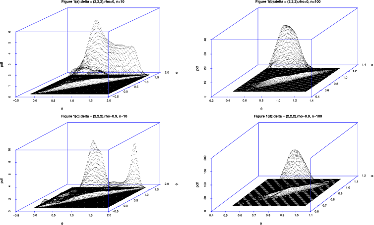
Figure 1: Plot of (simulated) polar angles.

4.2 Study design

The simulation study consists of three parts. In the first part we evaluate the accuracy and precision of $\hat{\mathbf{s}}_{\max}$ by estimating its bias and mean squared error (MSE). In the second part we investigate the coverage probability of bootstrap confidence intervals. In the third part we estimate type I errors and powers of the proposed test $S_{n,m}$ as well as the integral tests $I_{n,m}$ and $I_{n,m}^{+}$.

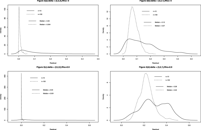
Figure 2: Plot of (simulated) polar residuals.

To evaluate the bias and MSEs we generated $\mathbf{X}_{1},\ldots,\mathbf{X}_{n}\sim N_{3}(\mathbf{0},\bolds{\Sigma})$ and $\mathbf{Y}_{1},\ldots,\mathbf{Y}_{m}\sim N_{3}(\bolds{\delta},\bolds{\Sigma})$ where $n=m=20$ or $100$ observations. The common variance matrix is assumed to have intra-class correlation structure, that is, $\bolds{\Sigma}=(1-\rho)\mathbf{I}+\rho\mathbf{J}$ where $\mathbf{I}$ is the identity matrix and $\mathbf{J}$ is a matrix of ones. Various patterns of the mean vectors $\bolds{\delta}$ and correlation coefficient $\rho$ were considered as described in Table 1.

We conducted extensive simulation studies to evaluate the performance of the bootstrap confidence intervals. In this paper we present a small sample of our study. We generated data from two 5-dimensional normal populations with means $\mathbf{0}$ and $\bolds{\delta}$, respectively, and a common covariance $\bolds{\Sigma}=(1-\rho)\mathbf{I}+\rho\mathbf{J}$. We considered 5 patterns of $\rho$ and 2 patterns of sample sizes ($n=m=20$ and $40$). The nominal coverage probability was $0.95.$ Results are summarized in Table 2.

=270pt $\bolds{\delta}$ $\bolds{\rho}$ Bias MSE $n=m=20$ $(1,1,1)$ $-0.25$ $0.001$ 0.072 $(1,1,1)$ $0$ $0.004$ 0.129 $(1,1,1)$ $0.25$ $0.009$ 0.187 $(1,1,1)$ $0.50$ $0.012$ 0.216 $(1,1,1)$ $0.90$ $0.010$ 0.203 $(3,2,1)$ $-0.25$ $0.018$ 0.090 $(3,2,1)$ $0$ $0.001$ 0.066 $(3,2,1)$ $0.25$ $0.053$ 0.114 $(3,2,1)$ $0.50$ $0.060$ 0.113 $(3,2,1)$ $0.90$ $0.112$ 0.170 $n=m=100$ $(1,1,1)$ $-0.25$ $0.00009$ 0.014 $(1,1,1)$ $0$ $0.00021$ 0.027 $(1,1,1)$ $0.25$ $0.00045$ 0.041 $(1,1,1)$ $0.50$ $0.00079$ 0.056 $(1,1,1)$ $0.90$ $0.00050$ 0.044 $(3,2,1)$ $-0.25$ $0.02400$ 0.039 $(3,2,1)$ $0$ $0.00004$ 0.012 $(3,2,1)$ $0.25$ $0.05200$ 0.065 $(3,2,1)$ $0.50$ $0.06400$ 0.077 $(3,2,1)$ $0.90$ $0.14100$ 0.158

Table 1: Bias and MSE of $\hat{\mathbf{s}}_{\max}$

=260pt Set up Coverage probability Pattern $\bolds{\rho}$ $\bolds{n=m=20}$ $\bolds{n=m=40}$ 1 $-0.25$ 0.981 0.971 1 $0$ 0.913 0.918 1 $0.25$ 0.916 0.933 1 $0.50$ 0.971 0.969 1 $0.90$ 0.993 0.989 2 $-0.25$ 0.982 0.967 2 $0$ 0.984 0.972 2 $0.25$ 0.986 0.978 2 $0.50$ 0.968 0.968 2 $0.90$ 0.950 0.954

Table 2: Coverage probabilities for the bootstrap confidence intervals for $p=5$ normal data. Pattern $i=1,2$ corresponds to $\bolds{\delta}_{1}=(0.1,0.25,0.5,0.75,0.9)$ and $\bolds{\delta}_{2}=(0.5,0.5,0.5,0.5,0.5)$

The goal of the third part of our simulation study is to evaluate the type I error and the power of the test (9). To evaluate the type I error three different baseline distributions for the two populations $\mathbf{X}$ and $\mathbf{Y}$ were employed as follows: $(1)$ both distributed as $N(\mathbf{0},\bolds{\Sigma})\mathbf{;}(2)$ both distributed as $\pi N(\mathbf{0},\bolds{\Sigma})+(1-\pi)N(\bolds{\delta},\bolds{\Sigma})$ with $\pi=0.2$ or $\pi=0.8\mathbf{;}$ and $(3)$ both distributed as $\exp(\mathbf{Z})=(\exp(Z_{1}),\ldots,\exp(Z_{p}))$ where $\mathbf{Z}$ follows a $N(\bolds{\delta},\bolds{\Sigma})$. We refer to this distribution as the multivariate lognormal distribution. Throughout the variance matrix is assumed to have the intra-class structure described above. Various patterns of the mean vectors $\bolds{\delta}$ and correlation coefficient $\rho$ the dimension $p$ were considered as described in Table 3. Sample sizes of $n=m=15$ or $25$ are reported.

=270pt Set up Type I error Distribution $\bolds{p}$ $\bolds{\rho}$ $\bolds{n=m=15}$ $\bolds{n=m=25}$ MVNs 3 $-0.25$ 0.041 0.037 MVNs 3 $0.00$ 0.023 0.044 MVNs 3 $0.25$ 0.037 0.033 MVNs 3 $0.50$ 0.027 0.032 MVNs 3 $0.90$ 0.031 0.036 MVNs 5 $-0.25$ 0.035 0.035 MVNs 5 $0.00$ 0.040 0.041 MVNs 5 $0.25$ 0.045 0.032 MVNs 5 $0.50$ 0.038 0.043 MVNs 5 $0.90$ 0.044 0.031 MV-LogN 3 $-0.25$ 0.025 0.040 MV-LogN 3 $0.00$ 0.038 0.049 MV-LogN 3 $0.25$ 0.025 0.027 MV-LogN 3 $0.50$ 0.028 0.037 MV-LogN 3 $0.90$ 0.026 0.034 MV-LogN 5 $-0.25$ 0.026 0.039 MV-LogN 5 $0.00$ 0.035 0.018 MV-LogN 5 $0.25$ 0.039 0.039 MV-LogN 5 $0.50$ 0.036 0.046 MV-LogN 5 $0.90$ 0.034 0.042 Mix-MVNs 3 $-0.25$ 0.032 0.040 Mix-MVNs 3 $0.00$ 0.038 0.028 Mix-MVNs 3 $0.25$ 0.039 0.032 Mix-MVNs 3 $0.50$ 0.036 0.035 Mix-MVNs 3 $0.90$ 0.041 0.028 Mix-MVNs 5 $-0.25$ 0.042 0.035 Mix-MVNs 5 $0.00$ 0.040 0.031 Mix-MVNs 5 $-0.25$ 0.041 0.028 Mix-MVNs 5 $0.50$ 0.034 0.040 Mix-MVNs 5 $0.90$ 0.042 0.036

Table 3: Type I errors for the proposed procedure withnominal level $\alpha=0.05$. Three types of distributions are considered: MVNs, MV-LogN (multivariate lognormal) and Mix-MVN (mixtures of MVNs)

Table 4: Type I errors and power for some settings with $p\geq n$. Here $n=m=10$ and $\bolds{\delta}_{1}$ has components $1/2$ and $\bolds{\delta}_{2}$ has components $i/p$

Type I error and power $\bolds{p\!=\!10},\,\bolds{n\!=\!m\!=\!10}$			Type I error and power $\bolds{p\!=\!20},\,\bolds{n\!=\!m\!=\!10}$
$\bolds{\delta}$	$\bolds{\rho}$	Type I error	$\bolds{\delta}$	$\bolds{\rho}$	Type I error
$\mathbf{0}$	0.00	$0.054$	$\mathbf{0}$	0.00	$0.081$
$\mathbf{0}$	0.25	$0.051$	$\mathbf{0}$	0.25	$0.050$
$\mathbf{0}$	0.50	$0.028$	$\mathbf{0}$	0.50	$0.046$
$\mathbf{0}$	0.90	$0.038$	$\mathbf{0}$	0.90	$0.048$
Power			Power
$\bolds{\delta}_{1}$	0.00	$0.83$	$\bolds{\delta}_{1}$	0.00	$0.97$
$\bolds{\delta}_{1}$	0.25	$0.48$	$\bolds{\delta}_{1}$	0.25	$0.53$
$\bolds{\delta}_{1}$	0.50	$0.26$	$\bolds{\delta}_{1}$	0.50	$0.42$
$\bolds{\delta}_{1}$	0.90	$0.20$	$\bolds{\delta}_{1}$	0.90	$0.22$
$\bolds{\delta}_{2}$	0.00	$0.98$	$\bolds{\delta}_{2}$	0.00	$0.98$
$\bolds{\delta}_{2}$	0.25	$0.80$	$\bolds{\delta}_{2}$	0.25	$0.59$
$\bolds{\delta}_{2}$	0.50	$0.67$	$\bolds{\delta}_{2}$	0.50	$0.43$
$\bolds{\delta}_{2}$	0.90	$0.71$	$\bolds{\delta}_{2}$	0.90	$0.40$

Power comparisons were carried out for data generated from $\mathbf{X}_{1},\ldots,\mathbf{X}_{n}\sim N_{p}(\mathbf{0},\bolds{\Sigma})$ and $\mathbf{Y}_{1},\ldots,\mathbf{Y}_{m}\sim N_{p}(\bolds{\delta},\bolds{\Sigma})$ where $p=3$ or $5$ and a variety of patterns for $\bolds{\delta}$ as described in Table 4. If Roy’s maximal separating direction (cf. Proposition 3.1) was known then a “natural gold standard” would be the test based on $\Psi_{n,m}(\mathbf{s}_{\max})$. We shall refer to this test as the true maximal direction (TMD) test. Clearly the TMD test cannot be used in practice since it involves the unknown direction $\mathbf{s}_{\max}$. Nevertheless the TMD test provides an upper bound for the power of the proposed test which uses the estimated direction. Hence we compute the efficiency of the proposed test relative to TMD test. An additional test, referred to as the RMD test is also compared. The RMD test has the same form but uses Roy’s maximal direction given by $\mathbf{S}^{-1}(\bar{\mathbf{Y}}-\bar{\mathbf{X}})$. As suggested by a reviewer we also evaluated the power of the two integral based tests, described in (3.5), which do not require the determination of the best separating direction.

Additionally, in Table 5 we evaluate the type I error and power of our test when $\mathbf{X}_{1},\ldots,\mathbf{X}_{n}\sim N_{p}(\mathbf{0},\bolds{\Sigma})$ and $\mathbf{Y}_{1},\ldots,\mathbf{Y}_{m}\sim N_{p}(\bolds{\delta},\bolds{\Sigma})$ and $n=m=p=10$ and $n=m=10$ and $p=20$ (i.e., $p<n$ set up). Note that in neither of these cases the standard Hotteling’s $T^{2}$ (or Roy’s largest root test) can be computed whereas the proposed test can be calculated.

Simulation results reported in this paper are based on 1000 simulation runs. Confidence sets are calculated using 1000 bootstrap samples. The bootstrap critical values for estimating type I error were based on 500 bootstrap samples. Since the results between 100 bootstrap samples and 500 bootstrap samples did not differ by much, all powers were estimated using 100 bootstrap samples.

4.3 Simulation results

The Bias and MSEs for the patterns considered are summarized in Table 1. It is clear that the bias decreases with the sample size as do the MSEs. We observe that the bias tends to be smaller under independence and negative dependence compared with positive dependence. It also tends to be smaller when the data are exchangeable. Although results are not presented, we evaluated squared bias and MSE for larger values of $p$ (e.g., $p=5,10$ and $20$) and as expected the total squared bias and total MSE increased with the dimension $p$.

In Table 2 we summarize the estimated coverage probabilities of the bootstrap confidence intervals when $p=5$. Our simulation study suggests that the proposed bootstrap methodology seems to perform better for larger sample sizes but rather poorly for smaller samples sizes.

Type I errors for different patterns considered in our simulation study are summarized in Table 3. Our simulation studies suggest that in every case the proposed bootstrap based test maintains the nominal level of 0.05. In general it is slightly conservative. The performance of the test is not affected by the shape of the underlying distribution. This is not surprising, owing to the nonparametric nature of the test. Furthermore, we evaluated the type I error of the proposed bootstrap test for testing the null hypothesis (8) for $p$ as large as $20$ with $n=m=10$ and discovered that the proposed test attains the nominal level of 0.05 even $n\leq p$. See Table 4. As commented earlier in the paper, Hotelling’s $T^{2}$ statistic cannot be applied here since the Wishart matrix is singular in this case. However, the proposed method is still applicable since the estimation of the best direction does not require the inversion of a matrix.

The power of tests (9) and (3.5) for various patterns considered in our simulation study are summarized in Table 5.

Table 5: Power comparisons of the two proposed test procedures with type I error of 0.050. Here $\bolds{\delta}_{1}=(0.1,0.5,0.9)$, $\bolds{\delta}_{2}=(0.1,0.25,0.5,0.75,0.9)$, $\bolds{\delta}_{3}=(0.5,0.5,0.5)$ and $\bolds{\delta}_{4}=(0.5,0.5,0.5,0.5,0.5)$

Power and RE % $\bolds{(n=m=15)}$
Set up			Directional tests			Integral tests
$\bolds{p}$	$\bolds{\delta}$	$\bolds{\rho}$	$\bolds{S_{n,m}}$	RMD test	TMD test	$\bolds{I_{n,m}}$	$\bolds{I_{n,m}^{+}}$
3	$\bolds{\delta}_{1}$	$-0.25$	0.79 (90%)	0.62 (71%)	0.88	0.89 (100%)	0.89 (100%)
3	$\bolds{\delta}_{1}$	$0.00$	0.64 (82%)	0.45 (57%)	0.78	0.68 (87%)	0.68 (87%)
3	$\bolds{\delta}_{1}$	$0.25$	0.53 (78%)	0.38 (56%)	0.68	0.54 (79%)	0.54 (79%)
3	$\bolds{\delta}_{1}$	$0.50$	0.51 (73%)	0.41 (59%)	0.70	0.47 (67%)	0.47 (67%)
3	$\bolds{\delta}_{1}$	$0.90$	0.62 (64%)	0.85 (99%)	0.97	0.40 (41%)	0.41 (42%)
5	$\bolds{\delta}_{2}$	$-0.25$	0.93 (95%)	0.74 (76%)	0.98	0.97 (99%)	0.97 (99%)
5	$\bolds{\delta}_{2}$	$0.00$	0.80 (87%)	0.56 (60%)	0.92	0.86 (93%)	0.86 (93%)
5	$\bolds{\delta}_{2}$	$0.25$	0.59 (73%)	0.39 (47%)	0.81	0.66 (81%)	0.66 (81%)
5	$\bolds{\delta}_{2}$	$0.50$	0.56 (67%)	0.42 (50%)	0.84	0.48 (57%)	0.48 (57%)
5	$\bolds{\delta}_{2}$	$0.90$	0.63 (64%)	0.88 (89%)	0.99	0.40 (40%)	0.40 (40%)
3	$\bolds{\delta}_{3}$	$-0.25$	0.74 (89%)	0.54 (64%)	0.83	0.83 (100%)	0.83 (100%)
3	$\bolds{\delta}_{3}$	$0.00$	0.56 (87%)	0.34 (53%)	0.64	0.59 (92%)	0.59 (92%)
3	$\bolds{\delta}_{3}$	$0.25$	0.42 (87%)	0.23 (48%)	0.49	0.46 (93%)	0.46 (93%)
3	$\bolds{\delta}_{3}$	$0.50$	0.33 (86%)	0.15 (40%)	0.38	0.37 (97%)	0.37 (97%)
3	$\bolds{\delta}_{3}$	$0.90$	0.27 (83%)	0.12 (38%)	0.32	0.27 (83%)	0.27 (83%)
5	$\bolds{\delta}_{4}$	$-0.25$	0.92 (95%)	0.65 (68%)	0.96	0.95 (99%)	0.95 (99%)
5	$\bolds{\delta}_{4}$	$0.00$	0.75 (90%)	0.43 (51%)	0.83	0.82 (99%)	0.82 (99%)
5	$\bolds{\delta}_{4}$	$0.25$	0.49 (87%)	0.20 (35%)	0.57	0.60 (100%)	0.60 (100%)
5	$\bolds{\delta}_{4}$	$0.50$	0.41 (90%)	0.16 (34%)	0.45	0.43 (100%)	0.43 (100%)
5	$\bolds{\delta}_{4}$	$0.90$	0.29 (92%)	0.10 (32%)	0.31	0.33 (100%)	0.33 (100%)

Table 5: (Continued)

Power and RE % $\bolds{(n=m=25)}$
Set up			Directional tests			Integral tests
$\bolds{p}$	$\bolds{\delta}$	$\bolds{\rho}$	$\bolds{S_{n,m}}$	RMD test	TMD test	$\bolds{I_{n,m}}$	$\bolds{I_{n,m}^{+}}$
3	$\bolds{\delta}_{1}$	$-0.25$	0.96 (98%)	0.90 (91%)	0.98	0.98 (100%)	0.98 (100%)
3	$\bolds{\delta}_{1}$	$0.00$	0.85 (92%)	0.72 (78%)	0.92	0.85 (92%)	0.86 (92%)
3	$\bolds{\delta}_{1}$	$0.25$	0.80 (88%)	0.69 (76%)	0.90	0.75 (83%)	0.75 (83%)
3	$\bolds{\delta}_{1}$	$0.50$	0.75 (84%)	0.67 (75%)	0.89	0.66 (74%)	0.66 (74%)
3	$\bolds{\delta}_{1}$	$0.90$	0.89 (89%)	0.98 (99%)	1.00	0.59 (59%)	0.61 (61%)
5	$\bolds{\delta}_{2}$	$-0.25$	1.00 (100%)	0.98 (98%)	1.00	1.00 (100%)	1.00 (100%)
5	$\bolds{\delta}_{2}$	$0.00$	0.96 (97%)	0.85 (86%)	0.99	0.98 (99%)	0.98 (99%)
5	$\bolds{\delta}_{2}$	$0.25$	0.85 (88%)	0.74 (76%)	0.97	0.83 (86%)	0.83 (86%)
5	$\bolds{\delta}_{2}$	$0.50$	0.81 (84%)	0.74 (77%)	0.96	0.70 (73%)	0.70 (73%)
5	$\bolds{\delta}_{2}$	$0.90$	0.90 (90%)	0.99 (100%)	1.00	0.57 (57%)	0.58 (58%)
3	$\bolds{\delta}_{3}$	$-0.25$	0.94 (96%)	0.85 (87%)	0.98	0.96 (98%)	0.96 (98%)
3	$\bolds{\delta}_{3}$	$0.00$	0.75 (92%)	0.57 (69%)	0.82	0.79 (96%)	0.79 (96%)
3	$\bolds{\delta}_{3}$	$0.25$	0.62 (89%)	0.39 (56%)	0.70	0.66 (94%)	0.66 (94%)
3	$\bolds{\delta}_{3}$	$0.50$	0.54 (90%)	0.31 (52%)	0.60	0.55 (92%)	0.55 (92%)
3	$\bolds{\delta}_{3}$	$0.90$	0.44 (90%)	0.20 (42%)	0.49	0.42 (86%)	0.42 (86%)
5	$\bolds{\delta}_{4}$	$-0.25$	0.99 (99%)	0.94 (94%)	1.00	1.00 (100%)	1.00 (100%)
5	$\bolds{\delta}_{4}$	$0.00$	0.94 (96%)	0.72 (74%)	0.97	0.97 (100%)	0.97 (100%)
5	$\bolds{\delta}_{4}$	$0.25$	0.71 (90%)	0.41 (52%)	0.79	0.79 (100%)	0.79 (100%)
5	$\bolds{\delta}_{4}$	$0.50$	0.58 (91%)	0.25 (39%)	0.63	0.64 (100%)	0.64 (100%)
5	$\bolds{\delta}_{4}$	$0.90$	0.42 (87%)	0.18 (36%)	0.49	0.46 (94%)	0.46 (94%)

As expected, in every case the power of the TMD test is higher than that of $S_{n,m}$ test and the RMD test. The $S_{n,m}$ test is almost always more powerful than the RMD test. The relative efficiency of $S_{n,m}$ compared to the TMD test is quite high in most cases. When $n=m=15$ the relative efficiency ranges between 65–95%. It is almost always above 90% when the sample size increases to 25 per group. In general the two integral tests had very similar power. They had larger power than $S_{n,m}$ when $\rho<0$. As $\rho$ increased, the power of $S_{n,m}$ improved relative to the two integral tests. Test (9) seems to perform better when the components of $\bolds{\delta}$ were unequal. We also note that when the integral tests outperform $S_{n,m}$ the difference is usually small, whereas the $S_{n,m}$ test can outperform the integral tests substantially. For example, observe pattern 2 where the powers of $S_{n,m}$ and $I_{n,m}$ are $0.93$ and $0.97$, respectively, when $\rho=-0.25$ and $0.63$ versus $0.40$ when $\rho=0.90$.

5 Illustration

Prior to conducting a two-year rodent cancer bioassay to evaluate the toxicity/carcinogenicity of a chemical, the National Toxicology Program (NTP) routinely conducts a 90-day pre-chronic dose finding study. One of the goals of the 90-day study is to determine the maximum tolerated dose (MTD) that can be used in the two-year chronic exposure study. Accurate determination of the MTD is critical for the success of the two-year cancer bioassay. Cancer bioassays are typically very expensive and time consuming. Therefore their proper design, that is, choosing the correct dosing levels, is very important. When the highest dose used in the two-year study exceeds the MTD, a large proportion of animals in the high dose group(s) may die well before the end of the study, and the data from such group(s) cannot be used reliably. This results in inefficiency and wasted resources.

Typically the NTP uses the 90-day study to determine the MTD on the basis of a large number of correlated endpoints that provide information regarding toxicity. These include body weight, organ weights, clinical chemistry (red blood cell counts, cell volume, hemoglobin, hematocrit, lymphocytes, etc.), histopathology (lesions in various target organs), number of deaths and so forth. The dose response data is analyzed for each variable separately using Dunnett’s or the Williams’s test (or their nonparametric versions, Dunn’s test and Shirley’s test, resp.). NTP combines results from all such analyses qualitatively and uses other biological and toxicological information when making decisions regarding the highest dose for the two-year cancer bioassay. Analyzing correlated variables one at a time may result in loss of information. The proposed methodology provides a convenient method to combine information from several outcome variables to make comparisons between groups.

We now illustrate our methodology by re-analyzing data obtained from a recent NTP study of the chemical Citral [NTP (2003)]. Citral is a flavoring agent that is widely used in a variety of food items. The NTP assigned a random sample of 10 male rats to the control group and 10 to the 1785 mg/kg dose group. Hematological and clinical chemistry measurements such as the number of platelets (in 1000 per l), urea nitrogen (UN) (in mg/dl), alkaline phosphatase (AP) (in IU/l) and bile acids (BA) (in mol/l) were recorded on each animal at the end of the study. The NTP performed univariate analysis on each of these variables and found no significant difference between the control and dose group except for the concentration of urea nitrogen which was increased in the high dose group. This increase was marginally significant at the $5\%$ level and not at all after correcting for multiplicity. We applied the proposed methodology to compare the control with the high-dose group (1785 mg/kg) in terms of all nonnegative linear combinations of the above mentioned four variables. We test the null hypothesis of no difference between the control and the high-dose group against the alternative that the high-dose group is stochastically larger (in the above four variables) than the control group. The resulting $p$-value based on 10,000 bootstrap samples was $0.025$, which is significant at a $5\%$ level of significance. The estimated value of $\mathbf{s}_{\max}$ was $(0.074,0.986,0.012,0.150)^{T}$ and the estimated 95% confidence region is given by $\{\mathbf{s}\in\mathcal{S}_{+}^{p-1}\dvtx\hat{\mathbf{s}}^{T}_{\max}\mathbf{s}\leq 0.93\}$. Hence the confidence set includes any $\mathbf{s}$ which is within $21.5^{\circ}$ degrees of $\hat{\mathbf{s}}_{\max}$. This is a relatively large set due to the small sample sizes. Clearly our methodology appears to be sensitive to detect statistical differences which were not noted by NTP. Furthermore, our methodology allows us to infer that indeed 1785 mg/kg dose group is larger in the multivariate stochastic order than the control group. This is a much stronger conclusion than the simple ordering of their means. Thus we believe that the proposed framework and methodology for studying ordered distributions can serve as a useful tool in toxicology and is also applicable to a wide range of other problems as alluded to in this paper.

6 Concluding remarks and some open problems

In many applications, researchers are interested in comparing two experimental conditions, for example, a treatment and a control group, in terms of a multivariate response. In classical multivariate analysis one addresses such problems by comparing the mean vectors using Hotelling’s $T^{2}$ statistic. The assumption of MVN, underlying Hotelling’s $T^{2}$ test, may not hold in practice. Moreover if the data is not MVN, then the comparison of population means may not always provide complete information regarding the differences between the two experimental groups. Secondly, Hotelling’s $T^{2}$ statistics are designed for two-sided alternatives and may not be ideal if a researcher is interested in one-sided, that is, ordered alternatives. Addressing such problems requires one to compare the two experimental groups nonparametrically in terms of the multivariate stochastic order. Such comparisons, however, are very high dimensional and not easy to perform.

In this article we circumvent this challenge by considering the notion of the linear stochastic order between two random vectors. The linear stochastic order is a “weak” generalization of the univariate stochastic order. The linear stochastic order is simple to interpret and has an intuitive appeal. Using this notion of ordering, we developed nonparametric directional inference procedures. Intuitively, the proposed methodology seeks to determine the direction that best separates two multivariate populations. Asymptotic properties of the estimated direction are derived. Our test based on the best separating direction may be viewed as a generalization of Roy’s classical largest root test for comparing several MVN populations. To the best of our knowledge this is the first general test for multivariate ordered distributions. Since in practice sample sizes are small, we use the bootstrap methodology for drawing inferences.

We illustrated the proposed methodology using a data obtained from a recent toxicity/carcinogenicity study conducted by the US National Toxicology Program (NTP) on the chemical Citral. A re-analysis of their 90-day data using our proposed methodology revealed a linear stochastic increase in platelets, urea nitrogen, alkaline phosphatase and bile acids in the high-dose group relative to the control group, which was not seen in the original univariate analysis conducted by the NTP. These findings suggest that the proposed methodology may have greater sensitivity than the commonly used univariate statistical procedures. Our methodology is sufficiently general since it is nonparametric and can be applied to discrete and/or continuous outcome variables. Furthermore, our methodology exploits the underlying dependence structure in the data, rather than analyzing one variable at a time.

We note that our example and some of our results pertain to continuous RVs. However, the methodology may be used, with appropriate modification (e.g., methods for dealing with ties) with discrete (or mixed) data with no problem. Although the focus of this paper has been the comparison of two multivariate vectors, in many applications, especially in dose response studies, researchers may be interested in determining trends (order) among several groups. Similarly to classical parametric order restricted inference literature, one could generalize the methodology developed in this paper to test for order restrictions among multiple populations. For example, one could extend the results to $K\geq 2$ RVs ordered by the simple ordering, that is, $\mathbf{X}_{1}\prec_{l\mbox{-}\mathrm{st}}\mathbf{X}_{2}\prec_{l\mbox{-}\mathrm{st}}\cdots\prec_{l\mbox{-}\mathrm{st}}\mathbf{X}_{K}$ or to RVs ordered by the tree ordering, that is, $\mathbf{X}_{1}\prec_{l\mbox{-}\mathrm{st}}\mathbf{X}_{j}$ where $j=2,\ldots,K$. As pointed out by a referee the hypotheses $H_{0}\dvtx\mathbf{X}\preceq_{\mathrm{st}}\mathbf{Y}$ versus $H_{1}\dvtx\mathbf{X}\nprec_{\mathrm{st}}\mathbf{Y}$ can also be formulated and tested using the approach described. First note that the null hypothesis implies $\Psi(\mathbf{s})\geq 1/2$ for all $\mathbf{s}\in\mathcal{S}_{+}^{p-1}$. On the other hand under the alternative there is an $\mathbf{s}\in\mathcal{S}_{+}^{p-1}$ for which $\Psi(\mathbf{s})<1/2$. Thus a test may be based on the statistic

$$N^{1/2}\bigl{(}\Psi_{n,m}(\hat{\mathbf{s}}_{\min})-1/2\bigr{)},$$

where $\hat{\mathbf{s}}_{\min}$ is the value which minimizes $\Psi_{n,m}(\mathbf{s})$. It is also clear that the least favorable configuration occurs when $\Psi(\mathbf{s})=1/2$ for all $\mathbf{s}\in\mathcal{S}_{+}^{p-1}$ which is equivalent to $\mathbf{X}=_{\mathrm{st}}\mathbf{Y}$.

We believe that the result obtained here may be useful beyond order restricted inference. Our simulation study suggests that our estimator of the best separating direction, that is, (6) may be useful even in the context of classical multivariate analysis where it may be viewed as a robust alternative to Roy’s classical estimate. Finally we note that the linear stochastic order may be useful in a variety of other statistical problems. For example, we believe that it provides a useful framework for linearly combining the results of several diagnostic markers. This is a well-known problem in the context of ROC curve analysis in diagnostic medicine.

Appendix: Proofs

Proof of Theorem 2.1 (i) Let $g\dvtx\mathbb{R}^{p}\rightarrow\mathbb{R}^{n}$ be an affine increasing function. Clearly $g(\mathbf{x})=\mathbf{v}+\mathbf{M}\mathbf{x}$ for some $n$ vector $\mathbf{v}$ and $n\times p$ matrix $\mathbf{M}$ with nonnegative elements. Thus for any $\mathbf{u}\in$ $\mathbb{R}_{+}^{n}$ we have $\mathbf{s}=\mathbf{M}^{T}\mathbf{u}\in$ $\mathbb{R}_{+}^{p}$. Hence

$$\mathbf{u}^{T}g(\mathbf{X})\!=\!\mathbf{u}^{T}(\mathbf{v}\!+\!\mathbf{MX})\!=\!\mathbf{u}^{T}\mathbf{v}\!+\!\mathbf{s}^{T}\mathbf{X}\preceq_{\mathrm{st}}\mathbf{u}^{T}\mathbf{v}\!+\!\mathbf{s}^{T}\mathbf{Y}\!=\!\mathbf{u}^{T}(\mathbf{v}\!+\!\mathbf{MY})\!=\!\mathbf{u}^{T}g(\mathbf{Y})$$

as required where the inequality holds because $\mathbf{X}\preceq_{l\mbox{-}\mathrm{st}}\mathbf{Y}$. (ii) Fix $I\in\{1,\ldots,\break p\}$. Let $\mathbf{X}=(\mathbf{X}_{I},\mathbf{X}_{\bar{I}})$, $\mathbf{Y}=(\mathbf{Y}_{I},\mathbf{Y}_{\bar{I}})$ where $\bar{I}$ is the complement of $I$ in $\{1,\ldots,p\}$. Further define $\mathbf{s}^{T}=(\mathbf{s}_{I}^{T},\mathbf{s}_{\bar{I}}^{T})$ where $\mathbf{s}\in$ $\mathbb{R}_{+}^{p}$, and set $\mathbf{s}_{\bar{I}}^{T}=0$. It follows that for all $\mathbf{s}_{I}\in\mathbb{R}^{\dim(I)}$ we have

$$\mathbf{s}_{I}^{T}\mathbf{X}_{I}=\mathbf{s}^{T}\mathbf{X}\preceq_{\mathrm{st}}\bolds{\mathbf{s}^{T}\mathbf{Y}=s}_{I}^{T}\mathbf{Y}_{I}$$

as required. (iii) Let $\phi\dvtx\mathbb{R}\rightarrow\mathbb{R}$ be any increasing function. Note that

$$\mathbb{E}\bigl{(}\phi\bigl{(}\mathbf{s}^{T}\mathbf{X}\bigr{)}\bigr{)}=\mathbb{E\bigl{(}E}\bigl{(}\phi\bigl{(}\mathbf{s}^{T}\mathbf{X}\bigr{)}|\mathbf{Z}\bigr{)}\bigr{)}\leq\mathbb{E\bigl{(}E}\bigl{(}\phi\bigl{(}\mathbf{s}^{T}\mathbf{Y}\bigr{)}|\mathbf{Z}\bigr{)}\bigr{)}=\mathbb{E}\bigl{(}\phi\bigl{(}\mathbf{s}^{T}\mathbf{Y}\bigr{)}\bigr{)}.$$

The inequality is a consequence of $\mathbf{X}|\mathbf{Z}=\mathbf{z}\preceq_{l\mbox{-}\mathrm{st}}\mathbf{Y}|\mathbf{Z}=\mathbf{z}$. Since $\phi$ is arbitrary it follows that $\mathbf{X}\preceq_{l\mbox{-}\mathrm{st}}\mathbf{Y}$ as required. (iv) Let $\mathbf{X}=(\mathbf{X}_{1},\ldots,\mathbf{X}_{n})$, and define $\mathbf{Y}$ similarly. Let $\mathbf{s}\in$ $\mathbb{R}_{+}^{p}$ where $p=p_{1}+\cdots+p_{n}$. Now

$$\mathbf{s}^{T}\mathbf{X}=\mathbf{s}_{1}^{T}\mathbf{X}_{1}+\cdots+\mathbf{s}_{n}^{T}\mathbf{X}_{n}\quad\mbox{and}\quad\mathbf{s}^{T}\mathbf{Y}=\mathbf{s}_{1}^{T}\mathbf{Y}_{1}+\cdots+\mathbf{s}_{n}^{T}\mathbf{Y}_{n}$$

by assumption $\mathbf{s}_{i}^{T}\mathbf{X}_{i}\preceq_{\mathrm{st}}\mathbf{s}_{i}^{T}\mathbf{Y}_{i}$ for $i=1,\ldots,n$. In addition $\mathbf{s}_{i}^{T}\mathbf{X}_{i}$ and $\mathbf{s}_{j}^{T}\mathbf{X}_{j}$ are independent for $i\neq j$. It follows from Theorem 1.A.3 in Shaked and Shanthikumar (2007) that $\mathbf{s}_{1}^{T}\mathbf{X}_{1}+\cdots+\mathbf{s}_{n}^{T}\mathbf{X}_{n}\preceq_{\mathrm{st}}\mathbf{s}_{1}^{T}\mathbf{Y}_{1}+\cdots+\mathbf{s}_{n}^{T}\mathbf{Y}_{n}$, that is, $\mathbf{X}\preceq_{l\mbox{-}\mathrm{st}}\mathbf{Y}$ as required. (v) By assumption $\mathbf{X}_{n}\Rightarrow\mathbf{X}$ and $\mathbf{Y}_{n}\Rightarrow\mathbf{Y}$ where the symbol $\Rightarrow$ denotes convergence in distribution. By the continuous mapping theorem $\mathbf{s}^{T}\mathbf{X}_{n}\Rightarrow\mathbf{s}^{T}\mathbf{X}$ and $\mathbf{s}^{T}\mathbf{Y}_{n}\Rightarrow\mathbf{s}^{T}\mathbf{Y}$. It follows that

$$\mathbb{P}\bigl{(}\mathbf{s}^{T}\mathbf{X}_{n}\geq t\bigr{)}\rightarrow\mathbb{P}\bigl{(}\mathbf{s}^{T}\mathbf{X}\geq t\bigr{)}\quad\mbox{and}\quad\mathbb{P}\bigl{(}\mathbf{s}^{T}\mathbf{Y}_{n}\geq t\bigr{)}\rightarrow\mathbb{P}\bigl{(}\mathbf{s}^{T}\mathbf{Y}\geq t\bigr{)}.$$ (11)

Moreover since $\mathbf{X}_{n}\preceq_{l\mbox{-}\mathrm{st}}\mathbf{Y}_{n}$ we have

$$\mathbb{P}\bigl{(}\mathbf{s}^{T}\mathbf{X}_{n}\geq t\bigr{)}\leq\mathbb{P}\bigl{(}\mathbf{s}^{T}\mathbf{Y}_{n}\geq t\bigr{)}\qquad\mbox{for all }n\in\mathbb{N}.$$ (12)

Combining (11) and (12) we have $\mathbb{P}(\mathbf{s}^{T}\mathbf{X}\geq t)\leq\mathbb{P}(\mathbf{s}^{T}\mathbf{Y}\geq t)$, that is, $\mathbf{X}\preceq_{l\mbox{-}\mathrm{st}}\mathbf{Y}$ as required.

Before proving Theorem 2.2, we provide a definition and a preliminary lemma.

Definition .1.

We say that the RV $\mathbf{X}$ has an elliptical distribution with parameters $\bolds{\mu}$ and $\bolds{\Sigma}$ and generator $\phi(\cdot)$, denoted $\mathbf{X}\sim E_{p}(\bolds{\mu},\bolds{\Sigma},\phi)$, if its characteristic function is given by $\exp(i\mathbf{t}^{T}\bolds{\mu})\phi(\mathbf{t}^{T}\bolds{\Sigma}\mathbf{t})$.

For this and other facts about elliptical distributions which we use in the proofs below, see Fang, Kots and Ng (1989).

Lemma .1.

Let $X\sim E_{1}(\mu,\sigma,\phi)$ and $Y\sim E_{1}(\mu^{\prime},\sigma^{\prime},\phi)$ be univariate elliptical RVs supported on $\mathbb{R}$. Then $X\preceq_{\mathrm{st}}Y$ if and only if $\mu\leq\mu^{\prime}$ and $\sigma=\sigma^{\prime}$.

Since $X$ and $Y$ have the same generator they have the stochastic representation:

$$X=_{\mathrm{st}}\mu+\sigma RU\quad\mbox{and}\quad Y=_{\mathrm{st}}\mu^{\prime}+\sigma^{\prime}RU,$$ (13)

where $R$ is a nonnegative RV, independent of the RV $U$, satisfying $\mathbb{P}(U=\pm 1)=1/2$; cf. Fang, Kots and Ng (1989). It follows that $RU$ is a symmetric RV supported on $\mathbb{R}$ with a strictly increasing DF which we denoted by $F_{0}$. Let $F_{X}$ and $F_{Y}$ denote the DFs of $X$ and $Y$, respectively. Note that $X\preceq_{\mathrm{st}}Y$ if and only if $F_{X}(t)\geq$ $F_{Y}(t)$ for all $t\in\mathbb{R}$, or equivalently by (13), if and only if

$$F_{0}\biggl{(}\frac{t-\mu}{\sigma}\biggr{)}\geq F_{0}\biggl{(}\frac{t-\mu^{\prime}}{\sigma^{\prime}}\biggr{)}$$ (14)

for all $t\in\mathbb{R}$. It is obvious that (14) holds when $\mu\leq\mu^{\prime}$ and $\sigma=\sigma^{\prime}$, establishing sufficiency. Now assume that $X\preceq_{\mathrm{st}}Y$. Put $t=\mu$ in (14), and use the strict monotonicity of $F_{0}$ to get $0\geq(\mu-\mu^{\prime})/\sigma^{\prime}$, that is, $\mu^{\prime}\geq\mu$. Suppose now that $\sigma^{\prime}>\sigma$. It follows from (14) and the the strict monotonicity of $F_{0}$ that $(t-\mu)/\sigma\geq(t-\mu^{\prime})/\sigma^{\prime}$ which is equivalent to $t\geq(\mu\sigma^{\prime}-\mu^{\prime}\sigma)/(\sigma^{\prime}-\sigma)$. The latter, however, contradicts the fact that (14) holds for all $t\in\mathbb{R}$. A similar argument shows that $\sigma^{\prime}<\sigma$ cannot hold; hence we must have $\sigma=\sigma^{\prime}$ as required.

Remark .1.

Note that Lemma .1 may not hold for distributions with a finite support. For example, if $R\sim U(0,1),$ then by (13) $X$ $\sim U(\mu-\sigma,\mu+\sigma)$ and $Y\sim U(\mu^{\prime}-\sigma^{\prime},\mu^{\prime}+\sigma^{\prime})$. It is easily verified that in this case $X\preceq_{\mathrm{st}}Y$ if and only if $\Delta=\mu^{\prime}-\mu\geq 0$ and $-\Delta\leq\sigma^{\prime}-\sigma\leq\Delta$; that is, it is not required that $\sigma=\sigma^{\prime}$. Hence the assumption that $X$ and $Y$ are supported on $\mathbb{R}$ is necessary.

We continue with the proof of Theorem 2.2. Proof of Theorem 2.2 Let $\mathbf{X}$ and $\mathbf{Y}$ be be $E_{p}(\bolds{\mu},\bolds{\Sigma},\phi)$ and $E_{p}(\bolds{\mu}^{\prime},\break\bolds{\Sigma}^{\prime},\phi)$ supported on $\mathbb{R}^{p}$. Suppose that $\mathbf{X}\preceq_{l\mbox{-}\mathrm{st}}\mathbf{Y}$. Choose $\mathbf{s}=\mathbf{e}_{i}$ where $\mathbf{e}_{ik}=1$ if $i=k$ and $0$ otherwise. It now follows from Definition 1.1 that $X_{i}\preceq_{\mathrm{st}}Y_{i}$. Since $X_{i}$ and $Y_{i}$ are marginally elliptically distributed RVs with the same generator and supported on $\mathbb{R},$ then by Lemma .1 we must have

$$\mu_{i}\leq\mu_{i}^{\prime}\quad\mbox{and}\quad\sigma_{ii}=\sigma_{ii}^{\prime}.$$ (15)

The latter holds, of course, for all $1\leq i\leq p$. Choosing $\mathbf{s}=\mathbf{e}_{i}+\mathbf{e}_{j}$ we have $X_{i}+X_{j}\preceq_{\mathrm{st}}Y_{i}+Y_{j}$. Note that $X_{i}+X_{j}$ and $Y_{i}+Y_{j}$ are supported on $\mathbb{R}$ and follow a univariate elliptical distribution with the same generator [Fang, Kots and Ng (1989)]. Applying Lemma .1 again we find that

$$\mu_{i}+\mu_{j}\leq\mu_{i}^{\prime}+\mu_{j}^{\prime}\quad\mbox{and}\quad\sigma_{ii}+\sigma_{jj}+2\sigma_{ij}=\sigma_{ii}^{\prime}+\sigma_{jj}^{\prime}+2\sigma_{ij}^{\prime}.$$ (16)

The latter holds, of course, for all $1\leq i\neq j\leq p$. It is easy to see that equations (15) and (16) imply that $\bolds{\mu}\leq\bolds{\mu}^{\prime}$ and $\bolds{\Sigma=\Sigma}^{\prime}$. Recall [cf. Fang, Kots and Ng (1989)] that we may write $\mathbf{X}=_{\mathrm{st}}\bolds{\mu}+R\mathbf{SU}$ and $\mathbf{Y}=_{\mathrm{st}}\bolds{\mu}^{\prime}+R\mathbf{SU}$ where $\bolds{\Sigma=S}^{T}\mathbf{S,}$ $\mathbf{U}$ is a uniform RV on $\mathcal{S}_{+}^{p-1}$, and $R$ is a nonnegative RV. Let $S$ be an upper set in $\mathbb{R}^{p}$. Clearly the set $[S-\bolds{\mu}]:=\{\mathbf{x}-\bolds{\mu}\dvtx x\in S\}$ is also an upper set and $[S-\bolds{\mu}]\subseteq[S-\bolds{\mu}^{\prime}]$ since $\bolds{\mu}\leq\bolds{\mu}^{\prime}$. Now,

$$\mathbb{P}(\mathbf{X}\in S)=\mathbb{P}\bigl{(}\mathbf{X}_{0}\in[S-\bolds{\mu}]\bigr{)}\leq\mathbb{P}\bigl{(}\mathbf{X}_{0}\in\bigl{[}S-\bolds{\mu}^{\prime}\bigr{]}\bigr{)}=\mathbb{P}(\mathbf{Y}\in S),$$

where $\mathbf{X}_{0}=R\mathbf{SU}$, hence $\mathbf{X}\preceq_{\mathrm{st}}\mathbf{Y}$. This proves the “if” part. The “only if” part follows immediately. Proof of Theorem 2.3 Let $\mathcal{X}_{p}=\{\mathbf{x}\dvtx(x_{1},\ldots,x_{p})\in\{0,1\}^{p}\}$ denote the support of a $p$-dimensional multivariate binary (MVB) RV. By definition the relationship $\mathbf{X}\preceq_{l\mbox{-}\mathrm{st}}\mathbf{Y}$ implies that for all $(t,\mathbf{s})\in\mathbb{R}_{+}\times\mathbb{R}_{+}^{p}$,

$$\mathbb{P}\bigl{(}\mathbf{s}^{T}\mathbf{X}>t\bigr{)}\leq\mathbb{P}\bigl{(}\mathbf{s}^{T}\mathbf{Y}>t\bigr{)}.$$ (17)

Now note that

$$\hskip 28.0pt\mathbb{P}\bigl{(}\mathbf{s}^{T}\mathbf{X}>t\bigr{)}=\sum_{\mathbf{x}\in\mathcal{X}_{p}}f(\mathbf{x})\mathbb{I}_{(\mathbf{s}^{T}\mathbf{x}>t)}\quad\mbox{and}\quad\mathbb{P}\bigl{(}\mathbf{s}^{T}\mathbf{Y}>t\bigr{)}=\sum_{\mathbf{x}\in\mathcal{X}_{p}}g(\mathbf{x})\mathbb{I}_{(\mathbf{s}^{T}\mathbf{x}>t)},$$ (18)

where $f$ and $g$ are the probability mass functions of $\mathbf{X}$ and $\mathbf{Y}$, respectively. Let $U$ be an upper set on $\mathcal{X}_{p}$. It is well known [cf. Davey and Priestley (2002)] that $U$ can be written as

$$U=\bigcup_{j\in J}U(\mathbf{x}_{j}),$$ (19)

where $\mathbf{x}_{j}$ are the distinct minimal elements of $U$, and $U(\mathbf{x}_{j})=\{\mathbf{x}\dvtx\mathbf{x}\geq\mathbf{x}_{j}\}$ are themselves upper sets [in fact $U(\mathbf{x}_{j})$ is an upper orthant]. The set $\{\mathbf{x}_{j}\dvtx$ $j\in J\}$ is often referred to as an anti-chain. Now observe that for any $\mathbf{s}\in\mathbb{R}_{+}^{p}$ the set $\{\mathbf{x}\dvtx\mathbf{s}^{T}\mathbf{x}>t\}$ is an upper set. Hence it must be of the form of (19) for some anti-chain $\{\mathbf{x}_{j}\dvtx$ $j\in J\}$. Suppose now, that for some $U\in\mathcal{X}_{p}$ there is a vector $\mathbf{s}_{U}\in\mathbb{R}_{+}^{p}$ such that $U=\{\mathbf{x}\dvtx\mathbf{s}_{U}^{T}\mathbf{x}>t\}$ for some fixed $t>0$. Then using (17) and (18) we have

$$\mathbb{P}(\mathbf{X}\in U) = \sum_{\mathbf{x}\in\{\mathbf{x}\dvtx\mathbf{s}_{U}^{T}\mathbf{x}>t\}}f(\mathbf{x})=\mathbb{P}\bigl{(}\mathbf{s}_{U}^{T}\mathbf{X}>t\bigr{)}\leq\mathbb{P}\bigl{(}\mathbf{s}_{U}^{T}\mathbf{Y}>t\bigr{)}$$

$$= \sum_{\mathbf{x}\in\{\mathbf{x}\dvtx\mathbf{s}_{U}^{T}\mathbf{x}>t\}}g(\mathbf{x})=\mathbb{P}(\mathbf{Y}\in U).$$

We will complete the proof by showing that for each upper set $U\in\mathcal{X}_{p}$, we can find a vector $\mathbf{s}_{U}$ for which $\mathbf{s}_{U}^{T}\mathbf{x}>t$ for $\mathbf{x}\in U$ and $\mathbf{s}_{U}^{T}\mathbf{x}\leq t$ for $\mathbf{x}\in U^{c}=\mathcal{X}\setminus U$ if and only if $p\leq 3$. To do so we will first solve the system of equations $\mathbf{s}^{T}\mathbf{x}_{j}=t$ for $j\in J$. This system can also be written as $\mathbf{X}\mathbf{s}=\mathbf{t}$ where

$$\mathbf{X}=\pmatrix{\mathbf{x}_{1}\cr\vdots\cr\mathbf{x}_{J}}$$

is a $J\times p$ matrix whose rows are the member of the anti-chain defining $U$, and $\mathbf{t}=(t,\ldots,t)$ has dimension $J$. Clearly the elements of $\mathbf{X}$ are ones and zeros. If $J\leq p$, the matrix $\mathbf{X}$ is of full rank since its rows are linearly independent by the fact that they are an anti-chain. Hence a solution for $\mathbf{s}$ exists. With a bit of algebra, we can further show that a solution $\mathbf{s}\geq 0$ exists. This, of course, is trivially verified when $p\leq 3$. Now set $\mathbf{s}_{U}=\mathbf{s}+\bolds{\varepsilon}$ for some $\bolds{\varepsilon}\geq 0$. It is clear that we can choose $\bolds{\varepsilon}$ small enough to guarantee that $\mathbf{s}_{U}^{T}\mathbf{x}>t$ if and only if $\mathbf{x}\in U$. Hence if $J\leq p$, upper set (19) can be mapped to a vector $\mathbf{s}_{U}$. However, the inequality $J\leq p$ for all upper sets $U\subset\mathcal{X}_{p}$ holds if and only if $p\leq 3$. This can be easily shown by enumerating all $18$ upper sets belonging to $\mathcal{X}_{3}$ [cf. Davidov and Peddada (2011)] and noting that they have at most three minimal elements. Hence if $p\leq 3$, then $\mathbf{X}\preceq_{l\mbox{-}\mathrm{st}}\mathbf{Y}$ $\Longleftrightarrow\mathbf{X}\preceq_{\mathrm{st}}\mathbf{Y}$ as required.

Now let $p=4$, and consider the upper set $U$ generated by the anti-chain $\mathbf{x}_{j}$, $j=1,\ldots,J$ where $\mathbf{x}_{j}$ are all the distinct permutations of the vector $(1,1,0,0)$. Clearly $J=6$. Note that although $J>p$, the system of equations $\mathbf{X}\mathbf{s}=\mathbf{t}$ is uniquely solved by $\mathbf{s}_{\ast}^{T}=(t/2,t/2,t/2,t/2)$. However, this solution coincides with the solution of the system $\mathbf{X}^{\prime}\mathbf{s}=\mathbf{t}$ where $\mathbf{X}^{\prime}$ is any matrix obtained from $\mathbf{X}$ by deleting any two (or just one) of its rows. Note that the rows of $\mathbf{X}^{\prime}$ correspond to an upper set $U^{\prime}\subset U$. This, in turn, implies that for any such $U^{\prime}$ one cannot find a vector $\mathbf{s}_{U^{\prime}}$ satisfying $\mathbf{s}_{U^{\prime}}^{T}\mathbf{x}>t$ if and only if $\mathbf{x}\in U^{\prime}$ because the inequality will hold for all $\mathbf{x}\in U$. Thus $U^{\prime}$ does not define an upper half plane. This shows that the linear stochastic order and the multivariate stochastic order do not coincide when $p=4$. A similar argument may be used for any $p\geq 5$. This completes the proof.

We first define the term copula.

Definition .2.

Let $F$ be the DF of a $p$-dimensional RV with marginal DFs $F_{1},\ldots,F_{p}$. The copula $C$ associated with $F$ is a DF such that

$$F(\mathbf{x})=C(\mathbf{x})=C\bigl{(}F_{1}(x_{1}),\ldots,F_{p}(x_{p})\bigr{)}.$$

It follows that the tail-copula $\bar{C}(\bolds{\cdot})$ is nothing but the tail of the DF $C(\bolds{\cdot})$.

Proof of Theorem 2.4 Suppose that $\mathbf{X}$ and $\mathbf{Y}$ have the same copula. Let $\mathbf{X}\preceq_{l\mbox{-}\mathrm{st}}\mathbf{Y}$. Choosing $\mathbf{s}=\mathbf{e}_{i}$ where $\mathbf{e}_{ik}=1$ if $i=k$ and $0$ otherwise, we find using the definition that $X_{i}\preceq_{\mathrm{st}}Y_{i}$. The latter holds, of course, for all $1\leq i\leq p$. Applying Theorem 6.B.14 in Shaked and Shanthikumar (2007), we find that $\mathbf{X}\preceq_{\mathrm{st}}\mathbf{Y}$. The reverse direction is immediate. Proof of Theorem 2.5 Note that for any $\mathbf{x}\in\mathbb{R}^{p}$ we have

$$F(\mathbf{x}) = C_{\mathbf{X}}\bigl{(}F_{1}(x_{1}),\ldots,F_{p}(x_{p})\bigr{)}\geq C_{\mathbf{X}}\bigl{(}G_{1}(x_{1}),\ldots,G_{p}(x_{p})\bigr{)}$$

$$\geq C_{\mathbf{Y}}\bigl{(}G_{1}(x_{1}),\ldots,G_{p}(x_{p})\bigr{)}=G(\mathbf{x}).$$

This means that $\mathbf{X}\preceq_{\mathrm{lo}}\mathbf{Y}$. The other part of the theorem is proved similarly. Proof of Proposition 3.1 Let $\mathbf{X}$ and $\mathbf{Y}$ be independent MVNs with means $\bolds{\mu}$ $\leq$ $\bolds{\nu}$ and common variance matrix $\bolds{\Sigma}$. Clearly

$$\mathbb{P}\bigl{(}\mathbf{s}^{T}\mathbf{X}\leq\mathbf{s}^{T}\mathbf{Y}\bigr{)}=\Phi\biggl{(}-\frac{\mathbf{s}^{T}(\bolds{\mu}-\bolds{\nu})}{\sqrt{2\mathbf{s}^{T}\bolds{\Sigma}\mathbf{s}}}\biggr{)},$$

where $\Phi$ is the DF of a standard normal RV. It follows that $\mathbb{P}(\mathbf{s}^{T}\mathbf{X}\leq\mathbf{s}^{T}\mathbf{Y})$ is maximized when the ratio $\mathbf{s}^{T}(\bolds{\nu-\mu})/\sqrt{\mathbf{s}^{T}\bolds{\Sigma}\mathbf{s}}$ is maximized. From the Cauchy–Schwarz inequality we have

$$\frac{\mathbf{s}^{T}(\bolds{\nu}-\bolds{\mu})}{\sqrt{\mathbf{s}^{T}\bolds{\Sigma}\mathbf{s}}}\leq\sqrt{(\bolds{\nu}-\bolds{\mu})^{T}\bolds{\Sigma}^{-1}(\bolds{\nu}-\bolds{\mu})}$$ (20)

for all $\mathbf{s}$. It is now easily verified that $\mathbf{s}=\bolds{\Sigma}^{-1}(\bolds{\nu-\mu})$ maximizes the left-hand side of (20). Proof of Proposition 3.2 Let $Q_{q}$, $q=1,\ldots,4$, be the four quadrants. It is clear that maximizing (2) is equivalent to maximizing

$$\Psi_{n,m}^{\prime}(\mathbf{s})=\sum_{\mathbf{Z}_{ij}\in Q_{2}}\mathbb{I}_{(\mathbf{s}^{T}\mathbf{Z}_{ij}\geq 0)}+\sum_{\mathbf{Z}_{ij}\in Q_{4}}\mathbb{I}_{(\mathbf{s}^{T}\mathbf{Z}_{ij}\geq 0)}.$$ (21)

It is also clear that for any $\mathbf{s}$ the indicators $\mathbb{I}_{(\mathbf{s}^{T}\mathbf{Z}_{ij}\geq 0)}$ are independent of the length of $\mathbf{Z}_{ij}$ which we therefore take to have length unity. Observe that the value of (21) is constant in the intervals $(\theta_{[i]},\theta_{[i+1]})$ where $\theta_{[i]}$ are defined in Algorithm 3.1. At each point $\theta_{[i]}$, $i=0,\ldots,M+1$, the value of (21) may increase or decrease. It follows that for all $\mathbf{s}\in\mathcal{S}_{+}^{p-1}$ $\Psi_{n,m}^{\prime}(\mathbf{s})\in\{\Psi_{n,m}^{\prime}(\mathbf{s}_{[0]}),\ldots,\Psi_{n,m}^{\prime}(\mathbf{s}_{[M+1]})\}$ where $\mathbf{s}_{[i]}$ are defined in Algorithm 3.1. Therefore the maximum value of (2) is an element of the above list. Now suppose that $\mathbf{s}_{[i]}$ is a global maximizer of (21). Clearly either $\Psi_{n,m}^{\prime}(\mathbf{s}_{[i]})=\Psi_{n,m}^{\prime}(\mathbf{s}_{[i-1]})$ or $\Psi_{n,m}^{\prime}(\mathbf{s}_{[i]})=\Psi_{n,m}^{\prime}(\mathbf{s}_{[i+1]})$ must hold, in which case any value in $[\theta_{[i-1]},\theta_{[i]}]$ or $[\theta_{[i]},\theta_{[i+1]}]$ is a global maximizer. This concludes the proof.  Proof of Theorem 3.1 Using Hajek’s projection and for any $\mathbf{s}$, we may write

$$\qquad\quad\Psi_{n,m}(\mathbf{s})=\Psi(\mathbf{s})+n^{-1}\sum_{i=1}^{n}\psi_{1}(\mathbf{X}_{i},\mathbf{s})+m^{-1}\sum_{j=1}^{m}\psi_{2}(\mathbf{Y}_{j},\mathbf{s})+R_{n,m}(\mathbf{s}),$$ (22)

where

$$\psi_{1}(\mathbf{X}_{i},\mathbf{s}) = \bar{G}\bigl{(}\mathbf{s}^{T}\mathbf{X}_{i}\bigr{)}-\Psi(\mathbf{s}),$$

$$\psi_{2}(\mathbf{Y}_{j},\mathbf{s}) = F\bigl{(}\mathbf{s}^{T}\mathbf{Y}_{j}\bigr{)}-\Psi(\mathbf{s})$$

and $R_{n,m}(\mathbf{s})$ is a remainder term. Here $\bar{G}(\mathbf{s}^{T}\mathbf{x})=\mathbb{P}(\mathbf{s}^{T}\mathbf{Y}\geq\mathbf{s}^{T}\mathbf{x})$, $F(\mathbf{s}^{T}\mathbf{y})=\mathbb{P}(\mathbf{s}^{T}\mathbf{X}\leq\mathbf{s}^{T}\mathbf{y})$ and $\Psi(\mathbf{s})=\mathbb{E}(\bar{G}(\mathbf{s}^{T}\mathbf{X}_{i}))=\mathbb{E}(F(\mathbf{s}^{T}\mathbf{Y}_{j}))$. Clearly $\mathbb{E}[\psi_{1}(\mathbf{X}_{i},\mathbf{s})]=\mathbb{E}[\psi_{2}(\mathbf{Y}_{j},\mathbf{s})]=0$ for all $i$ and $j$, so by the strong law of large numbers $n^{-1}\sum_{i=1}^{n}\psi_{1}(\mathbf{X}_{i},\mathbf{s})$ and $m^{-1}\sum_{j=1}^{m}\psi_{2}(\mathbf{Y}_{j},\mathbf{s})$ both converge to zero with probability one. Now,

$$\sup_{\mathbf{s}\in\mathcal{S}_{+}^{p-1}}\bigl{|}\Psi_{n,m}(\mathbf{s})-\Psi(\mathbf{s})\bigr{|} \leq \sup_{\mathbf{s}\in\mathcal{S}_{+}^{p-1}}\Biggl{|}n^{-1}\sum_{i=1}^{n}\psi_{1}(\mathbf{X}_{i},\mathbf{s})\Biggr{|}+\sup_{\mathbf{s}\in\mathcal{S}_{+}^{p-1}}\Biggl{|}m^{-1}\sum_{j=1}^{m}\psi_{2}(\mathbf{Y}_{j},\mathbf{s})\Biggr{|}$$

$${}+\sup_{\mathbf{s}\in\mathcal{S}_{+}^{p-1}}\bigl{|}R_{n,m}(\mathbf{s})\bigr{|}.$$

The set $\mathcal{S}_{+}^{p-1}$ is compact, and the function $\psi_{1}(\mathbf{x},\mathbf{s})$ is continuous in $\mathbf{s}\in\mathcal{S}_{+}^{p-1}$ for all values of $\mathbf{x}$ and bounded [in fact $|\psi_{1}(\mathbf{x},\mathbf{s})|\leq 2$]. Thus the conditions in Theorem 3.1 in DasGupta (2008) are satisfied, and it follows that $\sup_{\mathbf{s}\in\mathcal{S}_{+}^{p-1}}|n^{-1}\sum_{i=1}^{n}\psi_{1}(\mathbf{X}_{i},\mathbf{s})|\stackrel{{\scriptstyle\mathrm{a.s.}}}{{\rightarrow}}0$ as $n\rightarrow\infty$. Similarly $\sup_{\mathbf{s}\in\mathcal{S}_{+}^{p-1}}|m^{-1}\*\sum_{i=1}^{m}\psi_{2}(\mathbf{Y}_{i},\mathbf{s})|\stackrel{{\scriptstyle\mathrm{a.s.}}}{{\rightarrow}}0$ as $m\rightarrow\infty$. Since $\Psi_{n,m}(\mathbf{s})$ is bounded all its moments exist; therefore from Theorem 5.3.3 in Serfling (1980) we have that with probability one $R_{n,m}(\mathbf{s})=o(1/N)$. Moreover it is clear that the latter holds uniformly for all $\mathbf{s}$. Thus,

$$\sup_{\mathbf{s}\in\mathcal{S}_{+}^{p-1}}\bigl{|}\Psi_{n,m}(\mathbf{s})-\Psi(\mathbf{s})\bigr{|}\stackrel{{\scriptstyle\mathrm{a.s.}}}{{\rightarrow}}0\qquad\mbox{as }n,m\rightarrow\infty.$$

By assumption $\Psi(\mathbf{s}_{\max})>\Psi(\mathbf{s})$ for all $\mathbf{s}\in\mathcal{S}_{+}^{p-1}\setminus\mathbf{s}_{\max}$ so we can apply Theorem 2.12 in Kosorok (2008) to conclude that

$$\hat{\mathbf{s}}_{\max}\stackrel{{\scriptstyle\mathrm{a.s.}}}{{\rightarrow}}\mathbf{s}_{\max};$$

that is, $\hat{\mathbf{s}}_{\max}$ is strongly consistent. This completes the first part of the proof.

Since the densities of $\mathbf{X}$ and $\mathbf{Y}$ are differentiable, it follows that $\Psi(\mathbf{s})$ is continuous and twice differentiable. In particular at $\mathbf{s}_{\max}\in\mathcal{S}_{+}^{p-1}$, the matrix $-\nabla^{2}\Psi(\mathbf{s}_{\max})$ exists and is positive definite. A Taylor expansion implies that

$$\sup_{\|\mathbf{s}-\mathbf{s}_{\max}\|<\delta}\Psi(\mathbf{s})-\Psi(\mathbf{s}_{\max})\leq-C\delta^{2}.$$

It is also obvious that

$$n^{-1}\sum_{i=1}^{n}\psi_{1}(\mathbf{X}_{i},\mathbf{s}_{\max})=O_{p}(1/\sqrt{N})$$

and

$$m^{-1}\sum_{j=1}^{m}\psi_{2}(\mathbf{Y}_{j},\mathbf{s}_{\max})=O_{p}(1/\sqrt{N}).$$

Finally as noted above $|R_{n,m}(\mathbf{s})|=O(1/N)$ for all $\mathbf{s}$ as $n,m\rightarrow\infty$. Therefore by Theorem 1 in Sherman (1993) we have that

$$\hat{\mathbf{s}}_{\max}=\mathbf{s}_{\max}+O_{p}\bigl{(}N^{-1/2}\bigr{)};$$ (23)

that is, $\hat{\mathbf{s}}_{\max}$ converges to $\mathbf{s}_{\max}$ at a $N^{1/2}$ rate. This completes the second part of the proof.

The functions $\Psi(\mathbf{s}),\psi_{1}(\mathbf{X}_{i},\mathbf{s})$ and $\psi_{2}(\mathbf{Y}_{j},\mathbf{s})$ on the right-hand side of (22) all admit a quadratic expansion. A bit of algebra shows that for $\mathbf{s}$ in an $O_{p}(N^{-1/2})$ neighborhood of $\mathbf{s}_{\max}$, we have

$$\Psi_{n,m}(\mathbf{s}) = \Psi(\mathbf{s}_{\max})+(\mathbf{s}-\mathbf{s}_{\max})^{T}\frac{\mathbf{M}_{n,m}}{N^{1/2}}$$

$${}+\frac{1}{2}(\mathbf{s}-\mathbf{s}_{\max})^{T}\mathbf{V}(\mathbf{s}-\mathbf{s}_{\max})+o_{p}(1/N),$$

where

$$\mathbf{M}_{n,m}=\frac{1}{\sqrt{\lambda_{n,m}}}\frac{\sum_{i=1}^{n}\nabla\psi_{1}(\mathbf{X}_{i},\mathbf{s}_{\max})}{n^{1/2}}+\frac{1}{\sqrt{1-\lambda_{n,m}}}\frac{\sum_{j=1}^{m}\nabla\psi_{2}(\mathbf{Y}_{j},\mathbf{s}_{\max})}{m^{1/2}}$$

$\lambda_{n,m}=n/N$, for $j=1,2$ the function $\nabla\psi_{j}(\cdot,\mathbf{s}_{\max})^{T}$ is the gradient of $\psi_{j}(\cdot,\mathbf{s})$ evaluated at $\mathbf{s}_{\max}$, and the matrix $\mathbf{V}$ is given by

$$\mathbf{V}=\mathbb{E}\bigl{(}\nabla^{2}\psi_{1}(\mathbf{X},\mathbf{s}_{\max})\bigr{)}+\mathbb{E}\bigl{(}\nabla^{2}\psi_{2}(\mathbf{Y},\mathbf{s}_{\max})\bigr{)}.$$

Note that the $o_{p}(1/N)$ term in (Appendix: Proofs) absorbs $R_{n,m}(\mathbf{s})$ in (22) as well as the higher-order terms in the quadratic expansions of $\Psi(\mathbf{s}),n^{-1}\sum_{i=1}^{n}\psi_{1}(\mathbf{X}_{i},\mathbf{s})$ and $m^{-1}\sum_{j=1}^{m}\psi_{2}(\mathbf{Y}_{j},\mathbf{s})$. Now by the CLT and Slutzky’s theorem, we have that

$$\mathbf{M}_{n,m}\Rightarrow N(0,\bolds{\Delta}),$$

where

$$\bolds{\Delta} = \frac{1}{\lambda}\mathbb{E}\bigl{(}\nabla\psi_{1}(\mathbf{X},\mathbf{s}_{\max})\nabla\psi_{1}(\mathbf{X},\mathbf{s}_{\max})^{T}\bigr{)}$$

$${}+\frac{1}{1-\lambda}\mathbb{E}\bigl{(}\nabla\psi_{2}(\mathbf{Y},\mathbf{s}_{\max})\nabla\psi_{2}(\mathbf{Y},\mathbf{s}_{\max})^{T}\bigr{)}.$$

Finally it follows by Theorem 2 in Sherman (1993) that

$$N^{1/2}(\hat{\mathbf{s}}_{\max}-\mathbf{s}_{\max})\Rightarrow N(0,\bolds{\Sigma}),$$

where $\bolds{\Sigma}=\mathbf{V}^{-1}\bolds{\Delta V}^{-1}$, completing the proof. Proof of Theorem 3.2 Suppose that $\mathbf{X}$ and $\mathbf{Y}$ are discrete RVs with finite support. Let $p_{a}=\mathbb{P}(\mathbf{X}=\mathbf{x}_{a})>0$ and $q_{b}=\mathbb{P}(\mathbf{Y}=\mathbf{y}_{b})>0$ where $a=1,\ldots,A$ and $b=1,\ldots,B;$ $A$ and $B$ are finite. Define the set $\mathbf{S}_{ab}=\{\mathbf{s}\in\mathcal{S}_{+}^{p-1}\dvtx\mathbf{s}^{T}\mathbf{x}_{a}\leq\mathbf{s}^{T}\mathbf{y}_{b}\}$. A simple argument shows that

$$\Psi(\mathbf{s})=\mathbb{P}\bigl{(}\mathbf{s}^{T}\mathbf{X}\leq\mathbf{s}^{T}\mathbf{Y}\bigr{)}=\sum_{a=1}^{A}\sum_{b=1}^{B}\mathbb{I}_{(\mathbf{s}\in\mathbf{S}_{ab})}p_{a}q_{b}=\sum_{k=1}^{K}\alpha_{k}\mathbb{I}_{(\mathbf{s}\in\mathbf{S}_{k})},$$

where $K\leq 2^{AB}$ is finite, the sets $\mathbf{S}_{k}$ are distinct, $\bigcup_{k=1}^{K}\mathbf{S}_{k}=\mathcal{S}_{+}^{p-1}$ and $\alpha_{k}=\sum_{(a,b)\in J_{k}}p_{a}q_{b}$ with $J_{k}=\{(a,b)\dvtx\mathbf{S}_{k}\cap\mathbf{S}_{ab}\neq\varnothing\}$. Thus $\Psi(\mathbf{s})$ is a simple function on $\mathcal{S}_{+}^{p-1}$, and $\mathbf{S}_{\max}$ is the set associated with the largest $\alpha_{k}$. We will assume, without any loss of generality, that $\alpha_{1}>\alpha_{k}$ for all $k\geq 2$. Now note that

$$\Psi_{n,m}(\mathbf{s})=\frac{1}{nm}\sum_{i=1}^{n}\sum_{j=1}^{m}\mathbb{I}_{(\mathbf{s}^{T}\mathbf{X}_{i}\leq\mathbf{s}^{T}\mathbf{Y}_{j})}=\sum_{a=1}^{A}\sum_{b=1}^{B}\frac{n_{a}m_{b}}{nm}\mathbb{I}_{(\mathbf{s}\in\mathbf{S}_{ab})},$$

where $n_{a}=\sum_{i=1}^{n}\mathbb{I}_{(\mathbf{X}_{i}=\mathbf{x}_{a})},m_{b}=\sum_{j=1}^{m}\mathbb{I}_{(\mathbf{Y}_{i}=\mathbf{y}_{b})}$ where $a=1,\ldots,A$ and $b=1,\ldots,B$. Clearly $\Psi_{n,m}(\mathbf{s})$ is also a simple function. Moreover for large enough $n$ and $m$ we will have $n_{a}>0$ and $m_{b}>0$ for all $a=1,\ldots,A$ and $b=1,\ldots,B$, and consequently $\Psi_{n,m}(\mathbf{s})$ is defined over the same sets as $\Psi(\mathbf{s})$, that is,

$$\Psi_{n,m}(\mathbf{s})=\sum_{k=1}^{K}\hat{\alpha}_{k}\mathbb{I}_{(\mathbf{s}\in\mathbf{S}_{k})},$$

where $\hat{\alpha}_{k}=\sum_{(a,b)\in J_{k}}\hat{p}_{a}\hat{q}_{b}$ with $\hat{p}_{a}=n_{a}/n$ and $\hat{q}_{b}=m_{b}/m$. Furthermore the maximizer of $\Psi_{n,m}(\mathbf{s})$ is any $\mathbf{s}\in\mathbf{S}_{k}$ provided that $\mathbf{S}_{k}$ is associated with the largest $\hat{\alpha}_{k}$. Hence,

$$\mathbb{P}(\hat{\mathbf{s}}_{\max}\notin\mathbf{S}_{\max}) = \mathbb{P}\Bigl{(}\arg\max_{1\leq k\leq K}\hat{\alpha}_{k}\neq 1\Bigr{)}=\mathbb{P}\Biggl{(}\bigcup_{k=2}^{K}\{\hat{\alpha}_{1}\leq\hat{\alpha}_{k}\}\Biggr{)}$$

$$\leq \sum_{k=2}^{K}\mathbb{P}(\hat{\alpha}_{1}\leq\hat{\alpha}_{k})\leq(K-1)\max_{2\leq k\leq K}\mathbb{P}(\hat{\alpha}_{1}\leq\hat{\alpha}_{k}).$$

A bit of rearranging shows that

$$\mathbb{P}(\hat{\alpha}_{1}\leq\hat{\alpha}_{k}) = \mathbb{P}\biggl{(}\sum_{(a,b)\in J_{1}}\hat{p}_{a}\hat{q}_{b}-\sum_{(a,b)\in J_{k}}\hat{p}_{a}\hat{q}_{b}\leq 0\biggr{)}$$

$$= \mathbb{P}\Biggl{(}n^{-1}m^{-1}\sum_{i=1}^{n}\sum_{j=1}^{m}Z_{ij}^{(k)}\leq 0\Biggr{)},$$

where

$$Z_{ij}^{(k)}=\sum_{(a,b)\in J_{1}\setminus J_{k}}\mathbb{I}_{(\mathbf{X}_{i}=\mathbf{x}_{a})}\mathbb{I}_{(\mathbf{Y}_{j}=\mathbf{y}_{b})}-\sum_{(a,b)\in J_{k}\setminus J_{1}}\mathbb{I}_{(\mathbf{X}_{i}=\mathbf{x}_{a})}\mathbb{I}_{(\mathbf{Y}_{j}=\mathbf{y}_{b})}.$$

Note that $Z_{ij}^{(k)}$ may be viewed as a kernel of a two sample $U$-statistic. Moreover

$$-|J_{k}\setminus J_{1}|\leq Z_{ij}^{(k)}\leq|J_{k}\setminus J_{1}|$$

is bounded (here $|\cdot|$ denotes set cardinality) and $\mathbb{E}(Z_{ij}^{(k)})=\mu_{k}=\mathbb{E}(\hat{\alpha}_{1}-\hat{\alpha}_{k})>0$ by assumption. Applying Theorem 2 and the derivations in Section 5b in Hoeffding (1963) we have that

$$\mathbb{P}\Biggl{(}n^{-1}m^{-1}\sum_{i=1}^{n}\sum_{j=1}^{m}Z_{ij}^{(k)}\leq 0\Biggr{)}\leq\exp\biggl{(}-\frac{N\min(\lambda_{n,m},1-\lambda_{n,m})\mu_{k}^{2}}{2(|J_{k}\setminus J_{1}|+|J_{1}\setminus J_{k}|)^{2}}\biggr{)},$$ (26)

where $\lambda_{n,m}=n/N\rightarrow\lambda\in(0,1)$ as $n,m\rightarrow\infty$. Finally from (Appendix: Proofs) and (26) we have that

$$\mathbb{P}(\hat{\mathbf{s}}_{\max}\notin\mathbf{S}_{\max})\leq C_{1}\exp(-C_{2}N),$$

where $C_{1}=K-1$ and $C_{2}=\min(\lambda,1-\lambda)\min$ $2\mu_{k}^{2}(|J_{k}\setminus J_{1}|+|J_{1}\setminus J_{K}|)^{-2}$ completing the proof. Proof of Theorem 3.3 Choose $\varepsilon>0$. We have already seen that under the stated conditions, $\Psi(\mathbf{s})$ is continuous, and therefore for each $\mathbf{s}$ the set $B_{\mathbf{s},\varepsilon}=\{\mathbf{s}^{\prime}\dvtx|\Psi(\mathbf{s}^{\prime})-\Psi(\mathbf{s})|<\varepsilon\}$ is open. The collection $\{B_{\mathbf{s},\varepsilon}\dvtx\mathbf{s}\in\mathcal{S}_{+}^{p-1}\}$ is an open cover for $\mathcal{S}_{+}^{p-1}$. Since $\mathcal{S}_{+}^{p-1}$ is compact there exists a finite subcover $B_{\mathbf{s}_{1},\varepsilon},\ldots,B_{\mathbf{s}_{{}_{K}},\varepsilon}$ for $\mathcal{S}_{+}^{p-1}$ where $K<\infty$. Hence each $\mathbf{s}$ belongs to some $B_{\mathbf{s}_{{}_{i}},\varepsilon}$ and therefore

$$\sup_{\mathbf{s}\in\mathcal{S}_{+}^{p-1}}\bigl{|}\Psi_{N}(\mathbf{s})-\Psi(\mathbf{s})\bigr{|}$$

$$\qquad\leq\max_{1\leq i\leq K}\sup_{\mathbf{s}\in B_{\mathbf{s}_{i},\varepsilon}}\bigl{|}\Psi_{N}(\mathbf{s})-\Psi_{N}(\mathbf{s}_{i})\bigr{|}$$

$$\qquad\quad{}+\max_{1\leq i\leq K}\bigl{|}\Psi_{N}(\mathbf{s}_{i})-\Psi(\mathbf{s}_{i})\bigr{|}+\max_{1\leq i\leq K}\sup_{\mathbf{s}\in B_{\mathbf{s}_{i},\varepsilon}}\bigl{|}\Psi(\mathbf{s}_{i})-\Psi(\mathbf{s})\bigr{|}.$$

By construction $\sup_{\mathbf{s}\in B_{\mathbf{s}_{i},\varepsilon}}|\Psi(\mathbf{s}_{i})-\Psi(\mathbf{s})|<\varepsilon$ for all $i$. By the law of large numbers $\Psi_{N}(\mathbf{s}_{i})\stackrel{{\scriptstyle\mathrm{a.s.}}}{{\rightarrow}}\Psi(\mathbf{s}_{i})$ as $N\rightarrow\infty$ for each $i=1,\ldots,K$. Since $K$ is finite,

$$\max_{1\leq i\leq K}\bigl{|}\Psi_{N}(\mathbf{s}_{i})-\Psi(\mathbf{s}_{i})\bigr{|}\leq\sum_{i=1}^{K}\bigl{|}\Psi_{N}(\mathbf{s}_{i})-\Psi(\mathbf{s}_{i})\bigr{|}\stackrel{{\scriptstyle\mathrm{a.s.}}}{{\rightarrow}}0.$$

Now for any $\mathbf{s}^{\prime}\in B_{\mathbf{s}_{{}_{i}},\varepsilon}$, $\Psi_{N}(\mathbf{s}^{\prime})\stackrel{{\scriptstyle\mathrm{a.s.}}}{{\rightarrow}}\Psi(\mathbf{s}^{\prime})$, $\Psi_{N}(\mathbf{s}_{i})\stackrel{{\scriptstyle\mathrm{a.s.}}}{{\rightarrow}}\Psi(\mathbf{s}_{i})$ and $|\Psi(\mathbf{s}^{\prime})-\Psi(\mathbf{s}_{i})|<\varepsilon$. This implies that we can choose $N$ large enough so $|\Psi_{N}(\mathbf{s}^{\prime})-\Psi_{N}(\mathbf{s}_{i})|<2\varepsilon$. Moreover this bound holds for all $\mathbf{s}^{\prime}\in B_{\mathbf{s}_{{}_{i}},\varepsilon}$ and $i$ so

$$\lim\sup\bigl{|}\Psi_{N}(\mathbf{s})-\Psi(\mathbf{s})\bigr{|}\leq 3\varepsilon$$

on $\mathcal{S}_{+}^{p-1}$. Since $\varepsilon$ is arbitrary we conclude that $\sup_{\mathbf{s}\in\mathcal{S}_{+}^{p-1}}|\Psi_{N}(\mathbf{s})-\Psi(\mathbf{s})|\stackrel{{\scriptstyle\mathrm{a.s.}}}{{\rightarrow}}0$ as $N\rightarrow\infty$. By assumption $\Psi(\mathbf{s}_{\max})>\Psi(\mathbf{s})$ for all $\mathbf{s}\in\mathcal{S}_{+}^{p-1}\setminus\mathbf{s}_{\max}$, so we can apply Theorem 2.12 in Kosorok (2008) to conclude that

$$\hat{\mathbf{s}}_{\max}\stackrel{{\scriptstyle\mathrm{a.s.}}}{{\rightarrow}}\mathbf{s}_{\max},$$

that is, $\hat{\mathbf{s}}_{\max}$ is strongly consistent. This completes the first part of the proof.

We have already seen that

$$\sup_{\|\mathbf{s}-\mathbf{s}_{\max}\|<\delta}\Psi(\mathbf{s})-\Psi(\mathbf{s}_{\max})\leq-C\delta^{2}$$

holds. We now need to bound $\mathbb{E}^{\ast}\sup_{\|\mathbf{s}-\mathbf{s}_{\max}\|<\delta}N^{1/2}|(\mathbb{P}_{N}(\bar{\Psi}(\mathbf{s})-\bar{\Psi}(\mathbf{s}_{\max}))|$, where $\mathbb{E}^{\ast}$ denotes the outer expectation and $\bar{\Psi}(\mathbf{s})=\mathbb{I}_{(\mathbf{s}^{T}\mathbf{Z}\geq 0)}-\Psi(\mathbf{s})$. We first note that the bracketing entropy of the upper half-planes is of the order $\delta/\varepsilon^{2}$. The envelope function of the class $\mathbb{I}_{(\mathbf{s}^{T}\mathbf{z}\geq 0)}-\mathbb{I}_{(\mathbf{s}_{\max}^{T}\mathbf{z}\geq 0)}$ where $\|\mathbf{s}-\mathbf{s}_{\max}\|<\delta$ is bounded by $\mathbb{I}_{(\mathbf{s}^{T}\mathbf{z}\geq 0>\mathbf{s}_{\max}^{T}\mathbf{z})}+\mathbb{I}_{(\mathbf{s}_{\max}^{T}\mathbf{z}\geq 0>\mathbf{s}^{T}\mathbf{z})}$ whose squared $L_{2}$ norm is

$$\mathbb{P}\bigl{(}\mathbf{s}^{T}\mathbf{Z}\geq 0>\mathbf{s}_{\max}^{T}\mathbf{Z}\bigr{)}+\mathbb{P}\bigl{(}\mathbf{s}_{\max}^{T}\mathbf{Z}\geq 0>\mathbf{s}^{T}\mathbf{Z}\bigr{)}.$$ (27)

Note that we may replace the RV $\mathbf{Z}$ in (27) with the RV $\mathbf{Z}^{\prime}=\mathbf{Z}/\|\mathbf{Z}\|$ whose mass is concentrated on the unit sphere. The condition that $\|\mathbf{s}-\mathbf{s}_{\max}\|<\delta$ implies that the angle between $\mathbf{s}$ and $\mathbf{s}_{\max}$ is of the order $O(\delta),$ and therefore $\mathbb{P}(\mathbf{s}^{T}\mathbf{Z}^{\prime}\geq 0>\mathbf{s}_{\max}^{T}\mathbf{Z}^{\prime})$ is computed as surface integral on a spherical wedge with maximum width $\delta$. It follows that (27) is bounded by $2A_{p-1}\delta\|h^{\prime}\|_{\infty}$ where $A_{p-1}$ is the area of $\mathcal{S}_{+}^{p-1}$, and $\|h^{\prime}\|_{\infty}$ is the supremum of the density of $\mathbf{Z}^{\prime}$. Clearly $\|h^{\prime}\|_{\infty}<\infty$ since the density of $\mathbf{Z}$ is bounded by assumption. Thus by Corollary 19.35 in van der Vaart (2000) we have

$$\mathbb{E}^{\ast}\sup_{\|\mathbf{s}-\mathbf{s}_{\max}\|<\delta}N^{1/2}\bigl{|}\mathbb{P}_{N}\bigl{(}\bar{\Psi}(\mathbf{s})-\bar{\Psi}(\mathbf{s}_{\max})\bigr{)}\bigr{|}\leq C\delta^{1/2}.$$

It now follows that

$$\Psi_{N}(\hat{\mathbf{s}}_{\max})\geq\sup_{\mathbf{s}\in\mathcal{S}_{+}^{p-1}}\Psi_{N}(\mathbf{s})-o_{p}\bigl{(}N^{-2/3}\bigr{)},$$ (28)

which implies by Theorem 5.52 in van der Vaart (2000) and Theorem 14.4 of Kosorok (2008) that

$$\hat{\mathbf{s}}_{\max}=\mathbf{s}_{\max}+O_{p}\bigl{(}N^{-1/3}\bigr{)};$$

that is, $\hat{\mathbf{s}}_{\max}$ converges to $\mathbf{s}_{\max}$ at a cube root rate. This completes the second part of the proof.

The limit distribution is derived by verifying the conditions in Theorem 1.1 of Kim and Pollard (1990), denoted henceforth by KP. First note that (28) is condition (i) in KP. Since $\hat{\mathbf{s}}_{\max}$ is consistent, condition (ii) also holds, and condition (iii) holds by assumption. The differentiability of the density of $\mathbf{Z}$ implies that $\Psi(\mathbf{s})$ is twice differentiable. The uniqueness of the maximizer implies that $-\nabla^{2}\Psi(\mathbf{s}_{\max})$ is positive definite, and hence condition (iv) holds; see also Example 6.4 in KP for related calculations. Condition (v) in KP is equivalent to the existence of the limit $H(\mathbf{u},\mathbf{v})=\lim_{\alpha\rightarrow\infty}\alpha\mathbb{E}(\bar{\Psi}(\mathbf{s}_{\max}+\mathbf{u}/\alpha)\bar{\Psi}(\mathbf{s}_{\max}+\mathbf{v}/\alpha))$ which can be rewritten as

$$\lim_{\beta\rightarrow 0}\frac{1}{\beta}\bigl{[}\mathbb{P}\bigl{(}(\mathbf{s}_{\max}+\beta\mathbf{u})^{T}\mathbf{Z}\geq 0,(\mathbf{s}_{\max}+\beta\mathbf{v})^{T}\mathbf{Z}\geq 0\bigr{)}$$

$$\qquad\hskip 11.0pt{}-\mathbb{P}\bigl{(}(\mathbf{s}_{\max}+\beta\mathbf{u})^{T}\mathbf{Z}\geq 0\bigr{)}\mathbb{P}\bigl{(}(\mathbf{s}_{\max}+\beta\mathbf{v})^{T}\mathbf{Z}\geq 0\bigr{)}\bigr{]}.$$

With some algebra we find that this limit exists and equals

$$\int_{\mathbf{z}\in\mathcal{S}_{+}^{p-1}}\delta\bigl{(}\mathbf{s}_{\max}^{T}\mathbf{z}\bigr{)}\bigl{(}\mathbf{z}^{T}(\mathbf{u}+\mathbf{v})\bigr{)}h(\mathbf{z})\,d\mathbf{z}$$

$$\qquad{}-\int_{\mathbf{z}\in\mathcal{S}_{+}^{p-1}}\delta\bigl{(}\mathbf{s}_{\max}^{T}\mathbf{z}\bigr{)}\bigl{(}\mathbf{z}^{T}\mathbf{u}\bigr{)}h(\mathbf{z})\,d\mathbf{z}\int_{\mathbf{z}\in\mathcal{S}_{+}^{p-1}}\delta\bigl{(}\mathbf{s}_{\max}^{T}\mathbf{z}\bigr{)}\bigl{(}\mathbf{z}^{T}\mathbf{v}\bigr{)}h(\mathbf{z})\,d\mathbf{z},$$

where $\delta(\mathbf{s}_{\max}^{T}\mathbf{z})$ is the usual Dirac function; hence integration is with respect to the surface measure on $\{\mathbf{s}_{\max}^{T}\mathbf{z}=0\}$. It follows that condition also (v) holds. Conditions (vi) and (vii) were verified in the second part of the proof. Thus we may apply Theorem 1.1 in KP to get

$$N^{1/3}(\hat{\mathbf{s}}_{\max}-\mathbf{s}_{\max})\Rightarrow\arg\max\bigl{\{}-Q(\mathbf{s})+\mathbb{W}(\mathbf{s})\dvtx\mathbf{s}\in\mathcal{S}_{+}^{p-1}\bigr{\}},$$

where by KP $Q(\mathbf{s})=\mathbf{s}^{T}\nabla^{2}\Psi(\mathbf{s}_{\max})\mathbf{s}$ and $\mathbb{W}(\mathbf{s})$ is a zero mean Gaussian process with covariance function $H(\mathbf{u},\mathbf{v})$. This completes the proof. Proof of Proposition 3.3 Note that

$$\Psi(\mathbf{s}) = \mathbb{P}\bigl{(}\mathbf{s}^{T}\mathbf{X}\leq\mathbf{s}^{T}\mathbf{Y}\bigr{)}=\mathbb{P}\bigl{(}\mathbf{s}^{T}\mathbf{Z}\geq 0\bigr{)}=\mathbb{P}\biggl{(}\frac{\mathbf{s}^{T}\mathbf{Z}-\mathbf{s}^{T}\bolds{\delta}}{\sqrt{\mathbf{s}^{T}\bolds{\Sigma}\mathbf{s}}}\geq-\frac{\mathbf{s}^{T}\bolds{\delta}}{\sqrt{\mathbf{s}^{T}\bolds{\Sigma}\mathbf{s}}}\biggr{)}$$

$$= 1-F\biggl{(}-\frac{\mathbf{s}^{T}\bolds{\delta}}{\sqrt{\mathbf{s}^{T}\bolds{\Sigma}\mathbf{s}}}\biggr{)}.$$

Now, by assumption the DF $F$ is independent of $\mathbf{s}$. Therefore $\Psi(\mathbf{s})$ is uniquely maximized on $\mathcal{S}_{+}^{p-1}$ if and only if the function

$$\varkappa(\mathbf{s})=\frac{\mathbf{s}^{T}\bolds{\delta}}{\sqrt{\mathbf{s}^{T}\bolds{\Sigma}\mathbf{s}}}$$

is uniquely maximized on $\mathcal{S}_{+}^{p-1}$. If $\bolds{\Sigma=I}$, then $\varkappa(\mathbf{s})=\mathbf{s}^{T}\bolds{\delta}$, and we wish to maximize a linear function on $\mathcal{S}_{+}^{p-1}$. It is easily verified (by using ideas from linear programming) that the maximizer is unique if $\bolds{\delta}\geq\mathbf{0}$ which is true by assumption. Incidentally, it is easy to show directly that $\varkappa(\mathbf{s})$ is maximized at $\mathbf{s}^{\ast}/\|\mathbf{s}^{\ast}\|$ where

$$\mathbf{s}^{\ast}=(\delta_{1}\mathbb{I}_{(\delta_{1}\geq 0)},\ldots,\delta_{p}\mathbb{I}_{(\delta_{p}\geq 0)}).$$

Now let $\bolds{\Sigma}\neq\mathbf{I}$ and assume that a unique maximizer does not exist; that is, suppose that $\varkappa(\mathbf{s})$ is maximized by both $\mathbf{s}_{1}$ and $\mathbf{s}_{2}$. It is clear that $\varkappa(\lambda_{1}\mathbf{s}_{1})=\varkappa(\lambda_{2}\mathbf{s}_{2})$ for all $\lambda_{1},\lambda_{2}>0;$ that is, the value of $\varkappa(\cdot)$ is constant along rays through the origin. The rays passing through $\mathbf{s}_{1}$ and $\mathbf{s}_{2}$, respectively, intersect the ellipsoid $\mathbf{s}^{T}\bolds{\Sigma}\mathbf{s}=1$ at the points $\mathbf{p}_{1}$ and $\mathbf{p}_{2}$. It follows that $\varkappa(\mathbf{p}_{1})=\varkappa(\mathbf{p}_{2})$, moreover $\mathbf{p}_{1}$ and $\mathbf{p}_{2}$ maximize $\varkappa(\cdot)$ on the ellipsoid. Now since $\mathbf{p}_{1}^{T}\bolds{\Sigma}\mathbf{p}_{1}=1=\mathbf{p}_{2}^{T}\bolds{\Sigma}\mathbf{p}_{2}$ we must have $\mathbf{p}_{1}^{T}\bolds{\delta}=\mathbf{p}_{2}^{T}\bolds{\delta}$. Recall that a linear function on ellipsoid is uniquely maximized (just like on a sphere; see the comment above). Therefore we must have $\mathbf{p}_{1}=\mathbf{p}_{2}$ which implies that $\mathbf{s}_{1}=\mathbf{s}_{2}$ as required. Proof of Theorem 3.4 If $\mathbf{X}=_{\mathrm{st}}\mathbf{Y}$, then for all $\mathbf{s}$ we have $\mathbf{s}^{T}\mathbf{X}=_{\mathrm{st}}\mathbf{s}^{T}\mathbf{Y}$. By assumption both $\mathbf{s}^{T}\mathbf{X}$ and $\mathbf{s}^{T}\mathbf{Y}$ are continuous RVs, so $\mathbb{P}(\mathbf{s}^{T}\mathbf{X}\leq\mathbf{s}^{T}\mathbf{Y})=1/2$. Suppose now that both $\mathbf{X}\preceq_{\mathrm{st}}\mathbf{Y}$ and $\mathbb{P}(\mathbf{s}^{T}\mathbf{X}\leq\mathbf{s}^{T}\mathbf{Y})>1/2$ for some $\mathbf{s}\in\mathcal{S}_{+}^{p-1}$, hold. Then we must have $\mathbf{X}\prec_{l\mbox{-}\mathrm{st}}\mathbf{Y}$. Since $\mathbf{X}\preceq_{\mathrm{st}}\mathbf{Y}$ we have $X_{j}\preceq_{\mathrm{st}}Y_{j}$ for $1\leq j\leq p$. One of these inequalities must be strict; otherwise $\mathbf{X}=_{\mathrm{st}}\mathbf{Y}$ contradicts the fact that $\mathbf{X}\prec_{l\mbox{-}\mathrm{st}}\mathbf{Y}$. Now use Theorem 1 in Davidov and Peddada (2011) to complete the proof. Proof of Theorem 3.5 The functions $\psi_{1}$ and $\psi_{2}$ defined in the proof of Theorem 3.1 are Donsker; cf. Example 19.7 in van der Vaart (2000). Hence by the theory of empirical processes applied to (22), we find that

$$N^{1/2}\bigl{(}\Psi_{n,m}(\mathbf{s})-\Psi(\mathbf{s})\bigr{)}\Rightarrow\mathbb{G}(\mathbf{s}),$$ (29)

where $\mathbb{G}(\mathbf{s})$ is a zero mean Gaussian process, and convergence holds for all $\mathbf{s}\in\mathcal{S}_{+}^{p-1}$. We also note that (29) is a two-sample $U$-processes. A central limit theorem for such processes is described by Neumeyer (2004). Hence by the continuos mapping theorem, and under $H_{0}$, we have $N^{1/2}(\Psi_{n,m}(\hat{\mathbf{s}}_{\max})-1/2))\Rightarrow\sup_{\mathbf{s}\in\mathcal{S}_{+}^{p-1}}\mathbb{G}(\mathbf{s})$ where the covariance function of $\mathbb{G}(\mathbf{s})$, denoted by $C(\mathbf{u},\mathbf{v})$, is given by

$$\frac{1}{\lambda}\mathbb{P}\bigl{(}\mathbf{u}^{T}\mathbf{X}_{1}\leq\mathbf{u}^{T}\mathbf{X}_{2},\mathbf{v}^{T}\mathbf{X}_{1}\leq\mathbf{v}^{T}\mathbf{X}_{3}\bigr{)}$$

(30)

$$\qquad{}+\frac{1}{1-\lambda}\mathbb{P}\bigl{(}\mathbf{u}^{T}\mathbf{X}_{1}\leq\mathbf{u}^{T}\mathbf{X}_{2},\mathbf{v}^{T}\mathbf{X}_{3}\leq\mathbf{v}^{T}\mathbf{X}_{2}\bigr{)}-\frac{1}{4\lambda(1-\lambda)},$$

where $\mathbf{X}_{1},\mathbf{X}_{2},\mathbf{X}_{3}$ are i.i.d. from the common DF. Proof of Theorem 3.6 Suppose that $\mathbf{X}\prec_{l\mbox{-}\mathrm{st}}\mathbf{Y}$. Then for some $\mathbf{s}_{\ast}\in\mathcal{S}_{+}^{p-1}$ we have $\mathbf{s}_{\ast}^{T}\mathbf{X}\prec_{\mathrm{st}}\mathbf{s}_{\ast}^{T}\mathbf{Y}$ which implies that $\mathbb{P}(\mathbf{s}_{\ast}^{T}\mathbf{X}\leq\mathbf{s}_{\ast}^{T}\mathbf{Y})>1/2$. By definition $\mathbb{P}(\mathbf{s}_{\max}^{T}\mathbf{X}\leq\mathbf{s}_{\max}^{T}\mathbf{Y})\geq\mathbb{P}(\mathbf{s}_{\ast}^{T}\mathbf{X}\leq\mathbf{s}_{\ast}^{T}\mathbf{Y})$ so $\Psi(\mathbf{s}_{\max})>1/2$. It follows from the proof of Theorem 3.1 that $\Psi_{n,m}(\hat{\mathbf{s}}_{\max})\rightarrow\Psi(\mathbf{s}_{\max})$ with probability one. Thus,

$$S_{n,m}=N^{1/2}\bigl{(}\Psi_{n,m}(\hat{\mathbf{s}}_{\max})-1/2\bigr{)}\stackrel{{\scriptstyle\mathrm{a.s.}}}{{\longrightarrow}}\infty\qquad\mbox{as }n,m\rightarrow\infty.$$

Therefore by Slutzky’s theorem,

$$\mathbb{P}(S_{n,m}>q_{n,m,1-\alpha};H_{1})\rightarrow 1\qquad\mbox{as }n,m\rightarrow\infty,$$

where $q_{n,m,1-\alpha}$ is the critical value for an $\alpha$ level test based on samples of size $n$ and $m$ and $q_{n,m,1-\alpha}\rightarrow q_{1-\alpha}$. Hence the test based on $S_{n,m}$ is consistent. Consistency for $I_{n,m}$ and $I_{n,m}^{+}$ is established in a similar manner.

Now assume that $\mathbf{X}\preceq_{l\mbox{-}\mathrm{st}}\mathbf{Y}\preceq_{l\mbox{-}\mathrm{st}}\mathbf{Z}$ so that $\mathbf{s}^{T}\mathbf{Y}\preceq_{\mathrm{st}}\mathbf{s}^{T}\mathbf{Z}$ for all $\mathbf{s}\in\mathcal{S}_{+}^{p-1}$. Fix $\mathbf{x}_{i}$, $i=1,\ldots,n$, and choose $\mathbf{s}\in\mathcal{S}_{+}^{p-1}$. Without any loss of generality assume that $\mathbf{s}^{T}\mathbf{x}_{1}\leq$ $\mathbf{s}^{T}\mathbf{x}_{2}\leq\cdots\leq\mathbf{s}^{T}\mathbf{x}_{n}$. Define $U_{j}=\sum_{i=1}^{n}\mathbb{I}_{(\mathbf{s}^{T}\mathbf{x}_{i}\leq\mathbf{s}^{T}\mathbf{Y}_{j})}$ and $V_{j}=\sum_{i=1}^{n}\mathbb{I}_{(\mathbf{s}^{T}\mathbf{x}_{i}\leq\mathbf{s}^{T}\mathbf{Z}_{j})}$. Clearly $U_{j}$ and $V_{j}$ take values in $J=\{0,\ldots,n\}$. Now, for $k\in J$ we have

$$\mathbb{P}(U_{j}\geq k)=\mathbb{P}\bigl{(}\mathbf{s}^{T}\mathbf{Y}_{j}\geq\mathbf{s}^{T}\mathbf{x}_{k}\bigr{)}\leq\mathbb{P}\bigl{(}\mathbf{s}^{T}\mathbf{Z}_{j}\geq\mathbf{s}^{T}\mathbf{x}_{k}\bigr{)}=\mathbb{P}(V_{j}\geq k),$$

where we use the fact that $\mathbf{s}^{T}\mathbf{Y}\preceq_{\mathrm{st}}\mathbf{s}^{T}\mathbf{Z.}$ It follows that $U_{j}\preceq_{\mathrm{st}}V_{j}$ for $j=1,\ldots,m$. Moreover $\{U_{j}\}$ and $\{V_{j}\}$ are all independent and it follows from Theorem 1.A.3 in Shaked and Shanthikumar (2007) that $\sum_{j=1}^{m}U_{j}\preceq_{\mathrm{st}}\sum_{j=1}^{m}V_{j}$. Thus $\sum_{i=1}^{n}\sum_{j=1}^{m}\mathbb{I}_{(\mathbf{s}^{T}\mathbf{x}_{i}\leq\mathbf{s}^{T}\mathbf{Y}_{j})}\preceq_{\mathrm{st}}\sum_{i=1}^{n}\sum_{j=1}^{m}\mathbb{I}_{(\mathbf{s}^{T}\mathbf{x}_{i}\leq\mathbf{s}^{T}\mathbf{Z}_{j})}$. The latter holds for every value of $\mathbf{x}_{1},\ldots,\mathbf{x}_{n}$, and therefore it holds unconditionally as well, that is,

$$\sum_{i=1}^{n}\sum_{j=1}^{m}\mathbb{I}_{(\mathbf{s}^{T}\mathbf{X}_{i}\leq\mathbf{s}^{T}\mathbf{Y}_{j})}\preceq_{\mathrm{st}}\sum_{i=1}^{n}\sum_{j=1}^{m}\mathbb{I}_{(\mathbf{s}^{T}\mathbf{X}_{i}\leq\mathbf{s}^{T}\mathbf{Z}_{j})}.$$

It follows that $\Psi_{n,m}^{\mathbf{X},\mathbf{Y}}(\mathbf{s})\preceq_{\mathrm{st}}\Psi_{n,m}^{\mathbf{X},\mathbf{Z}}(\mathbf{s})$ for all $\mathbf{s}\in\mathcal{S}_{+}^{p-1}$ where $\Psi_{n,m}^{\mathbf{X},\mathbf{Y}}(\mathbf{s})$ and $\Psi_{n,m}^{\mathbf{X},\mathbf{Z}}(\mathbf{s})$ are defined in (2) and the superscripts emphasize the different arguments used to evaluate them. Thus

$$\Psi_{n,m}^{\mathbf{X},\mathbf{Y}}\bigl{(}\hat{\mathbf{s}}^{\mathbf{X},\mathbf{Y}}_{\max}\bigr{)}\preceq_{\mathrm{st}}\Psi_{n,m}^{\mathbf{X},\mathbf{Z}}\bigl{(}\hat{\mathbf{s}}^{\mathbf{X},\mathbf{Y}}_{\max}\bigr{)}\preceq_{\mathrm{st}}\Psi_{n,m}^{\mathbf{X},\mathbf{Z}}\bigl{(}\hat{\mathbf{s}}^{\mathbf{X},\mathbf{Z}}_{\max}\bigr{)}$$

and as a consequence $\mathbb{P}(S_{n,m}^{X,Y}>q_{n,m,1-\alpha})\leq\mathbb{P}(S_{n,m}^{X,Z}>q_{n,m,1-\alpha})$ as required. The monotonicity of the power function of $I_{n,m}$ and $I_{n,m}^{+}$ follows immediately from the fact that $\Psi_{n,m}^{\mathbf{X},\mathbf{Y}}(\mathbf{s})\preceq_{\mathrm{st}}\Psi_{n,m}^{\mathbf{X},\mathbf{Z}}(\mathbf{s})$ for all $\mathbf{s}\in\mathcal{S}_{+}^{p-1}$.

References

• Abrevaya and Huang (2005) {barticle}[mr] \bauthor\bsnmAbrevaya, \bfnmJason\binitsJ. and \bauthor\bsnmHuang, \bfnmJian\binitsJ. (\byear2005). \btitleOn the bootstrap of the maximum score estimator. \bjournalEconometrica \bvolume73 \bpages1175–1204. \biddoi=10.1111/j.1468-0262.2005.00613.x, issn=0012-9682, mr=2149245 \bptokimsref \endbibitem
• Arcones, Kvam and Samaniego (2002) {barticle}[mr] \bauthor\bsnmArcones, \bfnmMiguel A.\binitsM. A., \bauthor\bsnmKvam, \bfnmPaul H.\binitsP. H. and \bauthor\bsnmSamaniego, \bfnmFrancisco J.\binitsF. J. (\byear2002). \btitleNonparametric estimation of a distribution subject to a stochastic precedence constraint. \bjournalJ. Amer. Statist. Assoc. \bvolume97 \bpages170–182. \biddoi=10.1198/016214502753479310, issn=0162-1459, mr=1947278 \bptokimsref \endbibitem
• Audet, Béchard and Le Digabel (2008) {barticle}[mr] \bauthor\bsnmAudet, \bfnmCharles\binitsC., \bauthor\bsnmBéchard, \bfnmVincent\binitsV. and \bauthor\bsnmLe Digabel, \bfnmSébastien\binitsS. (\byear2008). \btitleNonsmooth optimization through mesh adaptive direct search and variable neighborhood search. \bjournalJ. Global Optim. \bvolume41 \bpages299–318. \biddoi=10.1007/s10898-007-9234-1, issn=0925-5001, mr=2398937 \bptokimsref \endbibitem
• Bekele and Thall (2004) {barticle}[mr] \bauthor\bsnmBekele, \bfnmB. Nebiyou\binitsB. N. and \bauthor\bsnmThall, \bfnmPeter F.\binitsP. F. (\byear2004). \btitleDose-finding based on multiple toxicities in a soft tissue sarcoma trial. \bjournalJ. Amer. Statist. Assoc. \bvolume99 \bpages26–35. \biddoi=10.1198/016214504000000043, issn=0162-1459, mr=2061885 \bptokimsref \endbibitem
• Bickel and Sakov (2008) {barticle}[mr] \bauthor\bsnmBickel, \bfnmPeter J.\binitsP. J. and \bauthor\bsnmSakov, \bfnmAnat\binitsA. (\byear2008). \btitleOn the choice of $m$ in the $m$ out of $n$ bootstrap and confidence bounds for extrema. \bjournalStatist. Sinica \bvolume18 \bpages967–985. \bidissn=1017-0405, mr=2440400 \bptokimsref \endbibitem
• DasGupta (2008) {bbook}[mr] \bauthor\bsnmDasGupta, \bfnmAnirban\binitsA. (\byear2008). \btitleAsymptotic Theory of Statistics and Probability. \bpublisherSpringer, \blocationNew York. \bidmr=2664452 \bptokimsref \endbibitem
• Davey and Priestley (2002) {bbook}[mr] \bauthor\bsnmDavey, \bfnmB. A.\binitsB. A. and \bauthor\bsnmPriestley, \bfnmH. A.\binitsH. A. (\byear2002). \btitleIntroduction to Lattices and Order, \bedition2nd ed. \bpublisherCambridge Univ. Press, \blocationNew York. \bidmr=1902334 \bptokimsref \endbibitem
• Davidov (2012) {barticle}[mr] \bauthor\bsnmDavidov, \bfnmOri\binitsO. (\byear2012). \btitleOrdered inference, rank statistics and combining $p$-values: A new perspective. \bjournalStat. Methodol. \bvolume9 \bpages456–465. \biddoi=10.1016/j.stamet.2011.10.003, issn=1572-3127, mr=2871445 \bptokimsref \endbibitem
• Davidov and Herman (2011) {barticle}[mr] \bauthor\bsnmDavidov, \bfnmOri\binitsO. and \bauthor\bsnmHerman, \bfnmAmir\binitsA. (\byear2011). \btitleMultivariate stochastic orders induced by case-control sampling. \bjournalMethodol. Comput. Appl. Probab. \bvolume13 \bpages139–154. \biddoi=10.1007/s11009-009-9136-4, issn=1387-5841, mr=2755136 \bptokimsref \endbibitem
• Davidov and Herman (2012) {barticle}[auto:STB—2013/01/29—08:09:18] \bauthor\bsnmDavidov, \bfnmO.\binitsO. and \bauthor\bsnmHerman, \bfnmA.\binitsA. (\byear2012). \btitleOrdinal dominance curve based inference for stochastically ordered distributions. \bjournalJ. R. Stat. Soc. Ser. B Stat. Methodol. \bvolume74 \bpages825–847. \bptokimsref \endbibitem
• Davidov and Peddada (2011) {barticle}[mr] \bauthor\bsnmDavidov, \bfnmOri\binitsO. and \bauthor\bsnmPeddada, \bfnmShyamal\binitsS. (\byear2011). \btitleOrder-restricted inference for multivariate binary data with application to toxicology. \bjournalJ. Amer. Statist. Assoc. \bvolume106 \bpages1394–1404. \biddoi=10.1198/jasa.2011.tm10322, issn=0162-1459, mr=2896844 \bptokimsref \endbibitem
• Delagdo, Rodriguez-Poo and Wolf (2001) {barticle}[auto:STB—2013/01/29—08:09:18] \bauthor\bsnmDelagdo, \bfnmMA\binitsM., \bauthor\bsnmRodriguez-Poo, \bfnmJ. M.\binitsJ. M. and \bauthor\bsnmWolf, \bfnmM.\binitsM. (\byear2001). \btitleSubsampling inference in cube root asymptotics with an application to Manski’s maximum score estimator. \bjournalEconom. Lett. \bvolume73 \bpages241–250. \bptokimsref \endbibitem
• Ding and Zhang (2004) {barticle}[mr] \bauthor\bsnmDing, \bfnmYing\binitsY. and \bauthor\bsnmZhang, \bfnmXinsheng\binitsX. (\byear2004). \btitleSome stochastic orders of Kotz-type distributions. \bjournalStatist. Probab. Lett. \bvolume69 \bpages389–396. \biddoi=10.1016/j.spl.2004.06.001, issn=0167-7152, mr=2091758 \bptokimsref \endbibitem
• Fang, Kots and Ng (1989) {bbook}[auto:STB—2013/01/29—08:09:18] \bauthor\bsnmFang, \bfnmK. T.\binitsK. T., \bauthor\bsnmKots, \bfnmS.\binitsS. and \bauthor\bsnmNg, \bfnmK. W.\binitsK. W. (\byear1989). \btitleSymmetric Multivariate and Related Distributions. \bpublisherChapman & Hall, \blocationLondon. \bptokimsref \endbibitem
• Fisher and Hall (1989) {barticle}[mr] \bauthor\bsnmFisher, \bfnmNicholas I.\binitsN. I. and \bauthor\bsnmHall, \bfnmPeter\binitsP. (\byear1989). \btitleBootstrap confidence regions for directional data. \bjournalJ. Amer. Statist. Assoc. \bvolume84 \bpages996–1002. \bidissn=0162-1459, mr=1134489 \bptokimsref \endbibitem
• Hájek, Šidák and Sen (1999) {bbook}[mr] \bauthor\bsnmHájek, \bfnmJaroslav\binitsJ., \bauthor\bsnmŠidák, \bfnmZbyněk\binitsZ. and \bauthor\bsnmSen, \bfnmPranab K.\binitsP. K. (\byear1999). \btitleTheory of Rank Tests, \bedition2nd ed. \bpublisherAcademic Press, \blocationSan Diego, CA. \bidmr=1680991 \bptokimsref \endbibitem
• Hoeffding (1963) {barticle}[mr] \bauthor\bsnmHoeffding, \bfnmWassily\binitsW. (\byear1963). \btitleProbability inequalities for sums of bounded random variables. \bjournalJ. Amer. Statist. Assoc. \bvolume58 \bpages13–30. \bidissn=0162-1459, mr=0144363 \bptokimsref \endbibitem
• Hu, Homem-de Mello and Mehrotra (2011) {bmisc}[auto:STB—2013/01/29—08:09:18] \bauthor\bsnmHu, \bfnmJ.\binitsJ., \bauthor\bsnmHomem-de-Mello, \bfnmT.\binitsT. and \bauthor\bsnmMehrotra, \bfnmS.\binitsS. (\byear2011). \bhowpublishedConcepts and applications of stochastically weighted stochastic dominance. Unpublished manuscript. Available at http://www.optimization-online.org/DB_FILE/2011/04/2981.pdf. \bptokimsref \endbibitem
• Ivanova and Murphy (2009) {barticle}[mr] \bauthor\bsnmIvanova, \bfnmAnastasia\binitsA. and \bauthor\bsnmMurphy, \bfnmMichael\binitsM. (\byear2009). \btitleAn adaptive first in man dose-escalation study of NGX267: Statistical, clinical, and operational considerations. \bjournalJ. Biopharm. Statist. \bvolume19 \bpages247–255. \biddoi=10.1080/10543400802609805, issn=1054-3406, mr=2518371 \bptokimsref \endbibitem
• Joe (1997) {bbook}[mr] \bauthor\bsnmJoe, \bfnmHarry\binitsH. (\byear1997). \btitleMultivariate Models and Dependence Concepts. \bpublisherChapman & Hall, \blocationLondon. \bidmr=1462613 \bptokimsref \endbibitem
• Johnson and Wichern (1998) {bbook}[auto:STB—2013/01/29—08:09:18] \bauthor\bsnmJohnson, \bfnmR.\binitsR. and \bauthor\bsnmWichern, \bfnmD.\binitsD. (\byear1998). \btitleApplied Multivariate Statistical Analysis. \bpublisherPrentice Hall, \blocationNew York. \bptokimsref \endbibitem
• Kim and Pollard (1990) {barticle}[mr] \bauthor\bsnmKim, \bfnmJeanKyung\binitsJ. and \bauthor\bsnmPollard, \bfnmDavid\binitsD. (\byear1990). \btitleCube root asymptotics. \bjournalAnn. Statist. \bvolume18 \bpages191–219. \biddoi=10.1214/aos/1176347498, issn=0090-5364, mr=1041391 \bptokimsref \endbibitem
• Kosorok (2008) {bbook}[mr] \bauthor\bsnmKosorok, \bfnmMichael R.\binitsM. R. (\byear2008). \btitleIntroduction to Empirical Processes and Semiparametric Inference. \bpublisherSpringer, \blocationNew York. \biddoi=10.1007/978-0-387-74978-5, mr=2724368 \bptokimsref \endbibitem
• Lee (1999) {barticle}[mr] \bauthor\bsnmLee, \bfnmStephen M. S.\binitsS. M. S. (\byear1999). \btitleOn a class of $m$ out of $n$ bootstrap confidence intervals. \bjournalJ. R. Stat. Soc. Ser. B Stat. Methodol. \bvolume61 \bpages901–911. \biddoi=10.1111/1467-9868.00209, issn=1369-7412, mr=1722246 \bptokimsref \endbibitem
• Lucas and Wright (1991) {barticle}[mr] \bauthor\bsnmLucas, \bfnmLarry A.\binitsL. A. and \bauthor\bsnmWright, \bfnmF. T.\binitsF. T. (\byear1991). \btitleTesting for and against a stochastic ordering between multivariate multinomial populations. \bjournalJ. Multivariate Anal. \bvolume38 \bpages167–186. \biddoi=10.1016/0047-259X(91)90038-4, issn=0047-259X, mr=1131713 \bptokimsref \endbibitem
• Moser (2000) {barticle}[auto:STB—2013/01/29—08:09:18] \bauthor\bsnmMoser, \bfnmV.\binitsV. (\byear2000). \btitleObservational batteries in neurotoxicity testing. \bjournalInternational Journal of Toxicology \bvolume19 \bpages407–411. \bptokimsref \endbibitem
• Neumeyer (2004) {barticle}[mr] \bauthor\bsnmNeumeyer, \bfnmNatalie\binitsN. (\byear2004). \btitleA central limit theorem for two-sample $U$-processes. \bjournalStatist. Probab. Lett. \bvolume67 \bpages73–85. \biddoi=10.1016/j.spl.2002.12.001, issn=0167-7152, mr=2039935 \bptokimsref \endbibitem
• NTP (2003) {bmisc}[pbm] \borganizationNTP (\byear2003). \bhowpublishedNTP toxicology and carcinogenesiss studies of citral (microencapsulated) (CAS No. 5392-40-5) in F344/N rats and B6C3F1 mice (feed studies). \bptokimsref \endbibitem
• Peddada (1985) {barticle}[mr] \bauthor\bsnmPeddada, \bfnmShyamal D.\binitsS. D. (\byear1985). \btitleA short note on Pitman’s measure of nearness. \bjournalAmer. Statist. \bvolume39 \bpages298–299. \biddoi=10.2307/2683708, issn=0003-1305, mr=0817793 \bptokimsref \endbibitem
• Peddada and Chang (1996) {barticle}[mr] \bauthor\bsnmPeddada, \bfnmShyamal Das\binitsS. D. and \bauthor\bsnmChang, \bfnmTed\binitsT. (\byear1996). \btitleBootstrap confidence region estimation of the motion of rigid bodies. \bjournalJ. Amer. Statist. Assoc. \bvolume91 \bpages231–241. \biddoi=10.2307/2291400, issn=0162-1459, mr=1394077 \bptokimsref \endbibitem
• Pitman (1937) {barticle}[auto:STB—2013/01/29—08:09:18] \bauthor\bsnmPitman, \bfnmE. J. G.\binitsE. J. G. (\byear1937). \btitleThe closest estimates of statistical parameters. \bjournalProceedings of the Cambridge Philosophical Society \bvolume33 \bpages212–222. \bptokimsref \endbibitem
• Price, Reale and Robertson (2008) {barticle}[mr] \bauthor\bsnmPrice, \bfnmC. J.\binitsC. J., \bauthor\bsnmReale, \bfnmM.\binitsM. and \bauthor\bsnmRobertson, \bfnmB. L.\binitsB. L. (\byear2008). \btitleA direct search method for smooth and non-smooth unconstrained optimization problems. \bjournalANZIAM J. \bvolume48 \bpages927–948. \bptokimsref \endbibitem
• Roy (1953) {barticle}[mr] \bauthor\bsnmRoy, \bfnmS. N.\binitsS. N. (\byear1953). \btitleOn a heuristic method of test construction and its use in multivariate analysis. \bjournalAnn. Math. Statist. \bvolume24 \bpages220–238. \bidissn=0003-4851, mr=0057519 \bptokimsref \endbibitem
• Sampson and Whitaker (1989) {barticle}[mr] \bauthor\bsnmSampson, \bfnmAllan R.\binitsA. R. and \bauthor\bsnmWhitaker, \bfnmLyn R.\binitsL. R. (\byear1989). \btitleEstimation of multivariate distributions under stochastic ordering. \bjournalJ. Amer. Statist. Assoc. \bvolume84 \bpages541–548. \bidissn=0162-1459, mr=1010343 \bptokimsref \endbibitem
• Sen, Banerjee and Woodroofe (2010) {barticle}[mr] \bauthor\bsnmSen, \bfnmBodhisattva\binitsB., \bauthor\bsnmBanerjee, \bfnmMoulinath\binitsM. and \bauthor\bsnmWoodroofe, \bfnmMichael\binitsM. (\byear2010). \btitleInconsistency of bootstrap: The Grenander estimator. \bjournalAnn. Statist. \bvolume38 \bpages1953–1977. \biddoi=10.1214/09-AOS777, issn=0090-5364, mr=2676880 \bptokimsref \endbibitem
• Serfling (1980) {bbook}[mr] \bauthor\bsnmSerfling, \bfnmRobert J.\binitsR. J. (\byear1980). \btitleApproximation Theorems of Mathematical Statistics. \bpublisherWiley, \blocationNew York. \bidmr=0595165 \bptokimsref \endbibitem
• Shaked and Shanthikumar (2007) {bbook}[mr] \bauthor\bsnmShaked, \bfnmMoshe\binitsM. and \bauthor\bsnmShanthikumar, \bfnmJ. George\binitsJ. G. (\byear2007). \btitleStochastic Orders. \bpublisherSpringer, \blocationNew York. \biddoi=10.1007/978-0-387-34675-5, mr=2265633 \bptokimsref \endbibitem
• Sherman (1993) {barticle}[mr] \bauthor\bsnmSherman, \bfnmRobert P.\binitsR. P. (\byear1993). \btitleThe limiting distribution of the maximum rank correlation estimator. \bjournalEconometrica \bvolume61 \bpages123–137. \biddoi=10.2307/2951780, issn=0012-9682, mr=1201705 \bptokimsref \endbibitem
• van der Vaart (2000) {bbook}[auto:STB—2013/01/29—08:09:18] \bauthor\bparticlevan der \bsnmVaart, \bfnmA. W.\binitsA. W. (\byear2000). \btitleAsymptotic Statistics. \bpublisherCambridge Univ. Press, \blocationCambridge. \bptokimsref \endbibitem