Bound states of dipolar molecules studied with the Berggren expansion method

Abstract

Bound states of dipole-bound negative anions are studied by using a non-adiabatic pseudopotential method and the Berggren expansion involving bound states, decaying resonant states, and non-resonant scattering continuum. The method is benchmarked by using the traditional technique of direct integration of coupled channel equations. A good agreement between the two methods has been found for well-bound states. For weakly-bound subthreshold states with binding energies comparable with rotational energies of the anion, the direct integration approach breaks down and the Berggren expansion method becomes the tool of choice.

I Introduction

Weakly-bound many-body systems are intensely studied in different domains of mesoscopic physics Riisager et al. (2000); Rotival et al. (2009), including nuclear Hansen and Jonson (1987); Tanihata (1996); Cobis et al. (1997); Jensen et al. (2004); Mazumdar et al. (2006), molecular Lim et al. (1977); Moiseyev and Corcoran (1979); Grisenti et al. (2000); D. Bressanini, G. Morosi, L. Bartini, and M. Mella, Few-Body Syst. 31, 199 () (2002); Li et al. (2006); Lefebvre et al. (2009), and atomic Mitroy (2005); Varga et al. (2008); Ferlaino and Grimm (2010) physics. In this context, dipolar anions are one of the most spectacular examples of marginally bound quantum systems Garrett (1970, 1971, 1980a, 1980b, 1981, 1982); L.G. Christophorou, Atomic and Molecular Radiation Physics, Wiley, New York () (1971); R.N. Compton, P.W. Reinhardt, and C.D. Cooper, J. Chem. Phys. 66, 3305 () (1977); Wong and Schulz (1974); Rohr and Linder (1976); Carlsten et al. (1976); Jordan and Luken (1976); Lykke et al. (1984); E. A. Brinkman, S. Berger, J. Marks, and J. I. Brauman, J. Chem. Phys. 99, 7586 () (1993); A. S. Mullin, K. K. Murray, C. P. Schulz, and W. C. Lineberger, J. Phys. Chem. 97, 10281 () (1993); C. Desfrançois, H. Abdoul-Carime, and J. P. Schermann, Int. J. Mol. Phys. B 10, 1339 () (1996); Smith et al. (1997); H. Abdoul-Carime and C. Desfrançois, Eur. Phys. J. D 2, 149 () (1998); S. Ard, W. R. Garrett, R. N. Compton, L. Adamowicz, and S. G. Stepanian, Chem. Phys. Lett. 473, 223 () (2009); Compton and Hammer (2001); Jordan and Wang (2003); Chernov et al. (2009).

The mechanism for forming anion states by the long-range dipolar potential has been proposed by Fermi and Teller Fermi and Teller (1947), who studied the capture of negatively charged mesons in matter. They found that if a negative meson is captured by a hydrogen nucleus, the binding energy of the electron becomes zero for the electric dipole moment of a meson-proton system ${{\mu}_{cr}=1.625}$ D. Later this result was generalized to the case of an extended dipole with an infinite moment of inertia Lévy-Leblond (1967). Lifting the adiabatic approximation by considering the rotational degrees of freedom of the anion Garrett (1970, 1971, 1980a, 1980b, 1981, 1982) turned out to be crucial; it also boosted the critical value of ${\mu}$ to about 2.5 D. For anions with ${\mu>{\mu}_{cr}}$, the number of bound states of the electron becomes finite, and the critical electric dipole moment ${{\mu}_{cr}}$ depends on the moment of inertia of the molecule. In the non-adiabatic calculations, the pseudo-potential was used to take into account finite size effects, repulsive core, polarization effects, and quadrupolar interaction. The pseudo-potential method has provided a convenient description of binding energy of the electron bound by an electric dipolar field. Recently, this method was applied to linear electric quadrupole systems Garrett (2008). Some recent theoretical studies of dipole-bound anions also employed the coupled cluster technique Kalcher and Sax (2000a, b); Skurski et al. (2002).

The unbound part of the spectrum of multipolar anions has been discussed theoretically in Refs. H. Estrada and W. Domcke, J. Phys. B 17, 279 () (1984); H. R. Sadeghpour, J. L. Bohn, M. J. Cavagnero, B. D. Esry, I. I. Fabrikant, J. H. Macek, and A. R. P. Rau, J. Phys. B 33, R93 () (2000) and Refs. quoted therein. Resonance energies of dipolar anions have been determined experimentally by low energy electron scattering off the dipolar molecules Wong and Schulz (1974); Rohr and Linder (1976); Lykke et al. (1984); A. S. Mullin, K. K. Murray, C. P. Schulz, and W. C. Lineberger, J. Phys. Chem. 97, 10281 () (1993); Smith et al. (1997).

Both the long-range dipole potential and the weak binding of dipolar anions provide a considerable challenge for theory. The impact of the molecular rotation on a weakly-bound electron can be represented by coupled-channel (CC) equations that can be solved by means of the direct integration. While this approach correctly predicts the number of bound states of polar anions, it is less precise for treatment of weakly-bound excited states. Moreover, it cannot be used for studies of dipolar anion resonances because the exact asymptotics for a dipolar potential in the presence of a molecular rotor cannot be determined.

In this paper, we apply the complex-energy configuration interaction framework based on the Berggren ensemble Berggren (1968) to the problem of bound states in dipole-bound negative anions. The Berggren completeness relation is a resonant-state expansion; it treats the resonant and scattering states on the same footing as bound states. We have successfully applied this tool to a variety of nuclear structure problems pertaining to weakly-bound and unbound nuclear states Michel et al. (2002, 2003); N. Michel, W. Nazarewicz, M. Płoszajczak, Phys. Rev. C, 70 064313 () (2004); Id Betan et al. (2002) (for a recent review see Ref. Michel et al. (2009)). The nuclear many-body realisation of the complex energy configuration interaction method is known under the name of the Gamow Shell Model.

Resonances do not belong to the Hilbert space, so the mathematical apparatus of quantum mechanics in Hilbert space is inadequate for Gamow states Gamow (1928), which are not square-integrable. It turned out that the mathematical structure of the Rigged Hilbert Space (RHS) I. M. Gel’fand and N. Ya. Vilenkin, Generalized functions, Vol. 4 , Academic Press , New-York () (1961); K. Maurin, Generalized Eigenfunction expansions and unitary representations of topological groups, Polish Scientific Publishers, Warsaw () (1968); A. Bohm, The rigged Hilbert space and quantum mechanics, Lecture Notes in Physics 78, Springer, New York () (1978) can accommodate time-asymmetric processes, such as particle decays, by extending the domain of quantum mechanics. The mathematical setting of the resonant state expansions follows directly from the formulation of quantum mechanics in the RHS I. M. Gel’fand and N. Ya. Vilenkin, Generalized functions, Vol. 4 , Academic Press , New-York () (1961); K. Maurin, Generalized Eigenfunction expansions and unitary representations of topological groups, Polish Scientific Publishers, Warsaw () (1968), rather than the usual Hilbert space A. Bohm, The rigged Hilbert space and quantum mechanics, Lecture Notes in Physics 78, Springer, New York () (1978); R. de la Madrid, Eur. J. Phys. 26, 287 () (2005); de la Madrid (2012).

The Berggren ensemble provides a natural generalization of the configuration interaction for the description of the particle continuum. The complex-energy Gamow-Siegert states Gamow (1928); A.F.J. Siegert, Phys. Rev. 56, 750 () (1939) states have been used in various contexts in nuclear, atomic, and molecular physics R.E. Peierls, Proc. R. Soc. A 253, 16 (1959)() (London); J. Humblet and L. Rosenfeld, Nucl. Phys. 26, 529 () (1961); Gyarmati and Kruppa (1986); Lind (1993); C.G. Bollini, O. Civitarese, A.L. De Paoli, and M.C. Rocca, Phys. Lett. B 382, 205 () (1996); R. de la Madrid, and M. Gadella, Am. J. Phys. 70, 626 () (2002); Hamilton and Greene (2002); E. Kapuścik, and P. Szczeszek, Czech. J. Phys. 53, 1053 () (2003); E. Hernandez, A. Járegui, and A. Mondragon, Phys. Rev. A 67, 022721 () (2003); E. Kapuścik, and P. Szczeszek, Found. Phys. Lett. 18, 573 () (2005); Santra et al. (2005); J. Julve, and F.J. de Urries, quant-ph/0701213 ; R. de la Madrid, quant-ph/0607168 ; Toyota et al. (2007). Some recent applications of Gamow-Siegert states, also in the context of a CC formalism relevant to the problem of dipole anions, can be found in, e.g., Refs. Kruppa et al. (2000); Barmore et al. (2000); Kruppa and Nazarewicz (2004); Tolstikhin (2006, 2008).

This paper is organized as follows. The Hamiltonian of the pseudo-potential method is briefly discussed in Sec. II. The CC formulation of the Schrödinger equation for dipole-bound negative anions is outlined in Sec. III. Section IV discusses the direct integration method (DIM) for solving the CC problem with a focus on difficulties in imposing proper boundary conditions when the rotational motion of the molecule is considered. The Bergggren expansion method (BEM) is introduced in Sec. V. Section VI specifies the coupling constants of the pseudo-potential and other calculation parameters. Salient features of DIM and BEM solutions are compared in Sec. VII. The predictions of DIM and BEM for low-lying energy states and r.m.s. radii of LiI^-, LiCl^-, LiF^-, and LiH^- anions are collected in Sec. VIII. Finally, Sec. IX contains the conclusions and outlook.

II Hamiltonian

A dipole-bound negative anion is composed of a neutral polar molecule with a dipole moment greater than ${\mu}_{cr}$ and a valence electron. The Hamiltonian of the total system can be written as:

$${H}_{tot}={H}_{e}+{H}_{mol}+{V}$$ (1)

where ${H}_{e}$ is the Hamiltonian of the valence electron, ${H}_{mol}$ is the Hamiltonian of the molecule, and $V$ is the electron-molecule interaction. The many-body Schrödinger equation for ${H}_{tot}$ couples all electrons of the system; hence, an approximation scheme has to be developed.

As a first simplification, we assume that the vibrational motion of a molecule is much slower than other modes so that it can be treated in the Born-Oppenheimer approximation. The Hamiltonian (1) simplifies considerably if one considers anions of closed-shell systems. Moreover, if spin is neglected Garrett (1982), the molecule can be treated as a rigid rotor. Note that the energy scales associated with the rotational motion of the molecule and the motion of the weakly-bound valence electron may be comparable. Consequently, there appears a strong non-adiabatic coupling between the molecular angular momentum $\bm{j}$ and the orbital angular momentum $\bm{\ell}$ of the electron. Eq. (1) thus writes within this approximation scheme:

$${H_{tot}}=\frac{\bm{p}_{e}^{2}}{2m_{e}}+\frac{\bm{j}^{2}}{2I}+{V}$$ (2)

where ${I}$ is the moment of inertia of the neutral molecule, ${\bm{p}_{e}}$ is the linear momentum of the valence electron and ${{m}_{e}}$ its mass. The interaction $V$ is approximated by a one-body pseudo-potential ${V(r,\theta)}$ acting on the valence electron Garrett (1978, 1979, 1982):

$$V(r,\theta)={V}_{\mu}(r,\theta)+{V}_{\alpha}(r,\theta)+{V}_{{Q}_{zz}}(r,\theta)+{V}_{\rm SR}(r),$$ (3)

where ${\theta}$ is the angle between the dipolar charge separation $\bm{s}$ and electron coordinate;

$${V}_{\mu}(r,\theta)=-\mu e\sum_{\lambda=1,3,\cdots}{\left(\frac{{r}_{<}}{{r}_{>}}\right)}^{\lambda}\frac{1}{s{r}_{>}}{P}_{\lambda}(\cos\theta)$$ (4)

is the dipole potential of the molecule;

$${V}_{\alpha}(r,\theta)=-\frac{e^{2}}{2{r}^{4}}\left[{\alpha}_{0}+{\alpha}_{2}{P}_{2}(\cos\theta)\right]f(r)$$ (5)

is the induced dipole potential, where ${{\alpha}_{0}}$ and ${{\alpha}_{2}}$ are the spherical and quadrupole polarizabilities of the linear molecule;

$${V}_{{Q}_{zz}}(r,\theta)=-\frac{e}{{r}^{3}}{Q}_{zz}{P}_{2}(\cos\theta)f(r)$$ (6)

is the potential due to the permanent quadrupole moment of the molecule; and a short-range potential

$${V}_{\rm SR}(r)={V}_{0}\exp(-{(r/{r}_{c})}^{6})$$ (7)

accounts for the exchange effects and compensates for spurious effects induced by the cut-off function

$$f(r)=1-\exp\{-{(r/r_{0})}^{6}\}$$ (8)

introduced in Eqs. (5,6) to avoid a singularity at ${r\to 0}$. The parameter $r_{0}$ in Eq. (8) is an effective short-range cutoff distance for the long-range interactions.

III Coupled-channel expression of the Hamiltonian

The eigenfunctions of the Hamiltonian (2) can be conveniently expressed in the CC representation:

$${\Psi}^{J}=\sum_{c}u_{c}^{J}(r)\Phi_{j_{c}\ell_{c}}^{J}$$ (9)

where the index $c$ labels the channel, $u_{c}^{J}(r)$ is the radial wave function of the valence electron in a channel $c$, and the channel function $\Phi_{j_{c}\ell_{c}}^{J}$ arises from the coupling of ${j}_{c}$ and ${\ell}_{c}$ to the total angular momentum $J$ of the anion: ${\bm{j}}+{\bm{\ell}}={\bm{J}}$. Due to rotational invariance of ${H}_{tot}$, its matrix elements are independent of the magnetic quantum number $M$, which will be omitted in the following.

The potential ${V(r,\theta)}$ in Eqs. (3 - 7) can be expanded in multipoles:

$$V(r,\theta)=\sum_{\lambda}V_{\lambda}(r)P_{\lambda}(\cos\theta),$$ (10)

where

$$P_{\lambda}(\cos\theta)=\frac{4\pi}{2\lambda+1}Y_{\lambda}^{(mol)}(\hat{\bm{s}})\cdot Y_{\lambda}^{(e)}(\hat{\bm{r}}).$$ (11)

The matrix elements of ${{P}_{\lambda}(\cos\theta)}$ between the channels $c$ and $c^{\prime}$ are obtained by means of the standard angular momentum algebra:

$$\braket{\Phi_{j_{c^{\prime}}\ell_{c^{\prime}}}^{J}}{P_{\lambda}(\cos\theta)}{\Phi_{j_{c}\ell_{c}}^{J}}$$ (12)

$$= {(-1)}^{j_{c^{\prime}}+j_{c}+J}\begin{Bmatrix}j_{c^{\prime}}&\ell_{c^{\prime}}&J\\ \ell_{c}&j_{c}&\lambda\end{Bmatrix}\begin{pmatrix}j_{c^{\prime}}&\lambda&j_{c}\\ 0&0&0\end{pmatrix}\begin{pmatrix}\ell_{c^{\prime}}&\lambda&\ell_{c}\\ 0&0&0\end{pmatrix}$$

$$\times \sqrt{(2\ell_{c^{\prime}}+1)(2\ell_{c}+1)(2j_{c^{\prime}}+1)(2j_{c}+1)}.$$

In the following, we express $r$ in units of the Bohr radius $a_{0}$, $I$ in units of $m_{e}a_{0}^{2}$, and energy in Ry. The radial functions $u_{c}^{J}(r)$ are solutions of the set of CC equations:

$$\left[\frac{d^{2}}{dr^{2}}-\frac{{\ell}_{c}({\ell}_{c}+1)}{{r}^{2}}-\frac{{j}_{c}({j}_{c}+1)}{I}+{E_{J}}\right]{u}_{c}^{J}(r)$$ (13)

$$= \sum_{c^{\prime}}v_{cc^{\prime}}^{J}(r)u_{c^{\prime}}^{J}(r),$$

where ${E_{J}}$ is the energy of the system and

$$v_{cc^{\prime}}^{J}(r)=\sum_{\lambda}\braket{\Phi_{j_{c^{\prime}}\ell_{c^{\prime}}}^{J}}{P_{\lambda}(\cos\theta)}{\Phi_{j_{c}\ell_{c}}^{J}}V_{\lambda}(r).$$ (14)

IV Direct integration of coupled-channel equations

The CC equations (13) can be solved by the DI method. Below we describe the method used to generate the channel wave functions $u_{c}(r)$ (from now on, the quantum number $J$ is omitted to simplify notation) obeying the physical boundary conditions. Namely, we assume that $u_{c}(r)$ is regular at origin: ${u}_{c}(r=0)=0$, and for ${r\rightarrow+\infty}$ it behaves like an outgoing wave ${u}_{c}^{+}(r)$.

The central issue of DI lies in the boundary condition at infinity. Indeed, as we shall see in Sec. (IV.2), an asymptotic wave function of a dipole-bound anion is not analytic in general, so that one cannot exactly impose outgoing boundary conditions. This calls for the use of controlled approximations. In the following, we describe the numerical integration of CC equations. While the method is standard (cf. Sec. 3.3.2 of Ref. Thompson (1988)), this particular application is not; hence key details should be given.

IV.1 The basis method with the direct integration

To integrate CC equations, we introduce the matching radius $r_{m}$ that defines the internal region $[0:r_{m}]$, where the centrifugal potential is appreciable, and the external zone $[r_{m}:+\infty]$. An internal basis function ${u}^{0}_{b;c}(r)$ in $[0:r_{m}]$ is regular at $r=0$:

$${u}^{0}_{b;c_{b}}(r)\sim{r}^{{\ell}_{{c}_{b}}+1}$$ (15)

in one channel ${c}_{b}=({j}_{{c}_{b}},{\ell}_{{c}_{b}})$. The CC equations imply that when $r\rightarrow 0$ the internal channel wave functions ${u}^{0}_{b;c}(r)$ with ${c\neq{c}_{b}}$ must behave as:

$$\frac{2m_{e}V_{cc_{b}}(0)}{\hbar^{2}}\times\left\{\begin{array}[]{l l}\frac{r^{\ell_{c_{b}}+3}}{2\ell_{c_{b}}+5}\ln(r/r_{m})&\text{for}~{}\ell_{c}=\ell_{c_{b}}+2,\\ \frac{r^{\ell_{c_{b}}+3}}{(\ell_{c_{b}}+2)(\ell_{c_{b}}+3)-\ell_{c}(\ell_{c}+1)}&~{}\text{otherwise.}\end{array}\right.$$

Note that is it necessary to pay attention when integrating CC equations close to ${r=s}$, as the potential (4) is not differentiable therein.

In the external region $[r_{m}:+\infty]$, the basis wave functions are denoted ${u}^{+}_{b;c_{b}}(r)$. By construction, at very large distances of the order of hundreds of $a_{0}$ (asymptotic region), ${u}^{+}_{b;c_{b}}(r)\neq 0$ for ${{c}_{b}=({j}_{{c}_{b}},{\ell}_{{c}_{b}})}$ and ${u}^{+}_{b;c}(r)=0$ for other channels ${c\neq{c}_{b}}$. The asymptotic behavior of external channel functions is discussed in Sec. IV.2 below.

Both sets of internal and external basis functions are used to expand the channel function $u_{c}(r)$:

$$u_{c}(r)=\left\{\begin{array}[]{l l}\sum_{b}C^{0}_{b}u^{0}_{b;c}(r)&\quad\text{for $r\leq r_{m}$},\\ \sum_{b}C^{+}_{b}u^{+}_{b;c}(r)&\quad\text{for $r\geq r_{m}$}\end{array}\right.$$ (16)

The matching conditions at ${r={r}_{m}}$

$$\sum_{b}\left[C^{0}_{b}u^{0}_{b;c}(r_{m})-C^{+}_{b}u^{+}_{b;c}(r_{m})\right] = 0,$$ (17)

$$\sum_{b}\left[C^{0}_{b}\frac{du^{0}_{b;c}}{dr}(r_{m})-C^{+}_{b}\frac{du^{+}_{b;c}}{dr}(r_{m})\right] = 0,$$ (18)

form a linear system of equations: ${AX=0}$. The condition of ${\det A=0}$ determines the energy of a bound or resonant state. (One can thus see that $\det A$ is thus the generalization of the Jost function for CC equations.) Once the eigenenergy has been found, the amplitudes ${C}^{0}_{b},{C}^{+}_{b}$ are given by the eigenvector ${X}$ of ${A}$. The overall norm is determined by the condition:

$$\sum_{c}\int_{0}^{+\infty}|u_{c}(r)|^{2}~{}dr=1.$$ (19)

IV.2 The coupled-channel equations in the asymptotic region

At large distances, ${{V}_{cc^{\prime}}(r)}$ can be written as:

$$V_{cc^{\prime}}(r)=\frac{\hbar^{2}}{2m_{e}}\left[\frac{\chi_{cc^{\prime}}}{r^{2}}+V_{3}(r)\right],$$ (20)

where $\chi_{cc^{\prime}}$ is a constant and ${V_{3}(r)}$ decreases for ${r\rightarrow+\infty}$ as $r^{-3}$. In the following, we shall assume that ${V_{3}(r)=0}$ in the asymptotic region. As the numerical integration up to ${r\sim 100~{}{a}_{0}}$ is stable, the error made by neglecting $V_{3}$ is around ${{10}^{-6}~{}{a}_{0}^{-3}}$, which is sufficiently small to insure that the asymptotic zone has been practically reached.

Let us first consider the case of an infinite moment of inertia $I\rightarrow+\infty$. Here, Eq. (13) becomes:

$$u^{\prime\prime}_{c}(r)=\frac{\ell_{c}(\ell_{c}+1)}{r^{2}}u_{c}(r)+\sum_{c^{\prime}}\frac{\chi_{cc^{\prime}}}{r^{2}}u_{c^{\prime}}(r)-k^{2}u_{c}(r),$$ (21)

where ${k=\sqrt{E}}$. The outgoing solution of (21) in a basis channel $b$ can be written in terms of spherical Hankel functions:

$$u^{+}_{b;c}(r)=g^{(b)}_{c}H^{+}_{\ell^{(b)}_{eff}}(kr),$$ (22)

where ${{\ell}^{(b)}_{eff}}$ is an effective angular momentum given by eigenvalues of the eigenproblem

$$\ell_{c}(\ell_{c}+1)g^{(b)}_{c}+\sum_{c^{\prime}}\chi_{cc^{\prime}}g^{(b)}_{c^{\prime}}=\ell^{(b)}_{eff}(\ell^{(b)}_{eff}+1)g^{(b)}_{c}.$$ (23)

Indeed, it immediately follows from Eqs. (21) and (23) that:

$$u^{+}_{b;c}(r)^{\prime\prime}=\left(\frac{\ell^{(b)}_{eff}(\ell^{(b)}_{eff}+1)}{r^{2}}-k^{2}\right)u^{+}_{b;c}(r),$$ (24)

so the physical interpretation of ${{\ell}^{(b)}_{eff}}$ in terms of an effective angular momentum is justified.

If ${I}$ is finite, however, solutions of Eq. (13) are no longer analytical at large distances. Nevertheless, it is possible to construct an adiabatic approximation for ${{u}_{c}(r)}$ in the asymptotic region. To this end, one defines the linear momentum ${{k}_{c}=\sqrt{E-{j}_{c}({j}_{c}+1)/I}}$ for a channel ${c}$. In the asymptotic region, Eq. (13) becomes:

$$u^{\prime\prime}_{c}(r)=\frac{\ell_{c}(\ell_{c}+1)}{r^{2}}u_{c}(r)+\sum_{c^{\prime}}\frac{\chi_{cc^{\prime}}}{r^{2}}u_{c^{\prime}}(r)-k_{c}^{2}u_{c}(r),$$ (25)

where, compared to Eq. (21), ${k}$ is replaced by the channel momentum ${{k}_{c}}$. This approximation can be applied if ${|E|\gg{j}_{c}({j}_{c}+1)/I}$ for all channels of importance. In those cases, one can introduce an ansatz for ${{u}_{c}(r)}$ by replacing ${k}$ by ${{k}_{c}}$ in Eq. (22). The relative error on a basis function ${{u}_{+}^{(b;c)}(r)}$ associated with this approximation is

$$\sum_{c^{\prime}}\left|\frac{\chi_{cc^{\prime}}}{r^{2}}\frac{g^{(b)}_{c^{\prime}}}{g^{(b)}_{c}}\left(\frac{H^{+}_{\ell^{(b)}_{eff}}(k_{c^{\prime}}r)}{H^{+}_{\ell^{(b)}_{eff}}(k_{c}r)}-1\right)\right|,$$ (26)

i.e., is of the order of ${|{k}_{c}-{k}_{c^{\prime}}|/{r}^{2}}$.

In practical calculations, ${I\sim{10}^{5}}$ and ${{j}_{max}\sim 7}$. This gives ${{j}_{max}({j}_{max}+1)/I\sim{10}^{-4}}$. Consequently, if ${|E|>{10}^{-3}}$ Ry, the error ${|{k}_{c}-{k}_{c^{\prime}}|/{r}^{2}<{10}^{-6}~{}{a}_{0}^{-3}}$ for ${r\sim 100~{}{a}_{0}}$ is close to that associated with the neglect of ${V_{3}(r)}$. On can thus see that the proposed ansatz accounts for the coupling term (20) in many cases. However, this approximation breaks down for weakly-bound/unbound states with $|E|<10^{-4}$ Ry; hence, a more adequate theoretical method based on a resonant state expansion needs to be introduced.

V Diagonalization with the Berggren basis

Another way to find eigenstates of the CC problem (13) is to diagonalize the associated Hamiltonian in a complete basis of single-particle states. Since our goal is to describe weakly-bound or unbound states, special care should be taken to treat the asymptotic part of wave functions as precisely as possible. A suitable basis for this problem is the one-body Berggren ensemble Berggren (1968); Berggren and Lind (1993); Lind (1993). This basis is generated by a finite-depth spherical potential and contains bound ($b$), decaying ($d$), and scattering ($s$) one-body states. Fot that reason, the Berggren ensemble is ideally suited to deal with structures having large spatial extensions (such as halos or Rydberg states) or outgoing behavior (such as decaying resonances). Some recent applications, in a many-body context, have been reviewed in Ref. Michel et al. (2009).

V.1 The Berggren basis

The finite-depth potential generating the Berggren ensemble can be chosen arbitrarily. To improve the convergence, however, it is convenient in practical applications to use a one-body potential, which is as close as possible to the Hartree-Fock field of the Hamiltonian in question. Therefore, in the case of the one-body problem (13), the most optimal potential to generate the Berggren basis is the diagonal part of ${{v}_{cc^{\prime}}(r)}$. This means that the basis states ${{\Phi}_{k,c}(r)}$ are eigenstates of the spherical potential ${{v}_{cc}(r)}$:

$$\Phi_{k,c}^{\prime\prime}(r)=\left(\frac{\ell_{c}(\ell_{c}+1)}{r^{2}}+v_{cc}(r)-k^{2}\right)\Phi_{k,c}(r)$$ (27)

that obey the following boundary conditions:

$$\!\!\!\!\!\!\!\!\!\Phi_{k,c}(r) \sim C^{0}r^{\ell_{c}+1},~{}r\sim 0~{}~{}\text{for all states},$$ (28)

$$\!\!\!\!\!\!\!\!\!\Phi_{k,c}(r) \sim C^{+}H^{+}_{\ell_{c}}(kr),~{}r\rightarrow+\infty\mbox{ (${b,d}$)},$$ (29)

$$\!\!\!\!\!\!\!\!\!\Phi_{k,c}(r) \sim C^{+}H^{+}_{\ell_{c}}(kr)+C^{-}H^{-}_{\ell_{c}}(kr),~{}r\rightarrow+\infty\mbox{ (${s}$)},$$ (30)

where the boundary conditions at ${r\sim 0}$ and at ${r\rightarrow+\infty}$ for scattering states (${s}$) are standard, and for bound and decaying states (${b,d}$) one imposes the outgoing boundary condition. Note that ${k}$ in Eq. (27) is in general complex.

The scattering states are normalized to the Dirac delta, which results in a condition for the $C^{-}$ and $C^{+}$ amplitudes in (30) Berggren (1968):

$$\braket{\Phi_{k,c}}{\Phi_{k^{\prime},c}}=\delta(k-k^{\prime})\Leftrightarrow 2\pi C^{+}C^{-}=1.$$ (31)

The normalization of bound states is standard as well, but that of decaying resonant states is not. Indeed, resonant states rapidly oscillate and diverge exponentially in modulus along the real ${r}$-axis; hence, one cannot calculate their norm in the same way as for the bound states.

The solution of this problem is provided by the exterior complex scaling Gyarmati and Vertse (1971), i.e., one calculates the norm of the resonant state using complex ${r}$ radii:

$$\braket{\Phi_{k,c}}{\Phi_{k,c}} = \int_{0}^{R}\Phi^{2}_{k,c}(r)\,dr$$ (32)

$$+ \int_{0}^{+\infty}\Phi^{2}_{k,c}(R+xe^{i\theta})\,e^{i\theta}\,dx,,$$

where ${R}$ is a radius taken sufficiently large so that condition (29) is fulfilled. In the above formula, ${\theta}$ is an angle of rotation chosen so that ${{\Phi}_{k,c}(R+x{e}^{i\theta})\rightarrow 0}$ for ${x\rightarrow+\infty}$, which is always possible provided ${\theta}$ is larger than a critical value depending on $k$ N. Michel, W. Nazarewicz, M. Płoszajczak, and J. Okołowicz, Phys. Rev. C 67, 054311 () (2003). Note that no modulus enters Eq. (32). This arises from the finite-lifetime character of resonant states, which requires us to use the biorthogonal scalar product J. Aguilar and J.M. Combes, Commun. Math. Phys. 22, 269 () (1971); E. Balslev, J.M. Combes, Commun. Math. Phys. 22, 280 () (1971); B. Simon, Commun. Math. Phys. 27, 1 () (1972); N. Michel, W. Nazarewicz, M. Płoszajczak, and J. Okołowicz, Phys. Rev. C 67, 054311 () (2003); Michel et al. (2009). It can be shown J. Aguilar and J.M. Combes, Commun. Math. Phys. 22, 269 () (1971); E. Balslev, J.M. Combes, Commun. Math. Phys. 22, 280 () (1971); B. Simon, Commun. Math. Phys. 27, 1 () (1972) that the norm defined in Eq. (32) is indeed independent of ${R}$ and ${\theta}$, as expected from a norm. Since the expression (32) is also valid for bound states, bound and decaying states enter the Berggren ensemble as one family of resonant states.

The exterior complex scaling can be used to calculate matrix elements of a one-body operator ${O(r)}$ as well, provided it decreases faster than ${1/r}$ along the complex ${r}$-contour:

$$\braket{\Phi_{k^{\prime},c^{\prime}}}{O}{\Phi_{k,c}}=\int_{0}^{R}\Phi_{k^{\prime},c^{\prime}}(r)~{}O_{cc^{\prime}}(r)~{}\Phi_{k,c}(r)\,dr$$ (33)

$$+ \int_{0}^{+\infty}\!\!\!\!\!\Phi_{k^{\prime},c^{\prime}}(z(x))~{}O_{cc^{\prime}}(z(x))~{}\Phi_{k,c}(z(x))\,e^{i\theta}\,dx,$$

where ${z(x)=R+x{e}^{i\theta}}$, and ${\ket{{\Phi}_{k,c}}}$ and ${\ket{{\Phi}_{k^{\prime},c^{\prime}}}}$ can here be bound, decaying, or scattering states.

V.2 The Berggren completeness relation

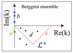
Figure 1: Berggren ensemble in the complex momentum plane. The bound ($b$) and antibound ($a$) states are distributed along the imaginary ${k}$-axis at ${Im(k)>0}$ and ${Im(k)<0}$, respectively. The decaying resonant states ($d$) are located in the fourth quadrant (${Re(k)>0},{Im(k)<0}$. The Berggren completeness relation involves bound states, scattering states ($s$) on the ${{\cal L}^{+}}$ contour, and decaying states lying between the real-$k$ axis and ${{\cal L}^{+}}$. If antibound states are included, the ${{\cal L}^{+}}$ contour has to be slightly deformed Michel et al. (2006, 2009). If the contour ${{\cal L}^{+}}$ lies on the real ${k}$-axis, the Berggren completeness relation reduces to the Newton completeness relation Michel et al. (2009); Newton (1982) involving bound and real-energy scattering states.

Figure 1 shows a distribution the Berggren ensemble in the complex momentum plane. To determine the basis, one first chooses a ${{\cal L}^{+}}$ contour in the fourth quadrant containing the decaying eigenstates. The scattering states of the ensemble lie on this contour. The resonant part of the ensemble contains the bound states lying on the imaginary-$k$ axis and those decaying states of (27) that are found in the region between the real-${k}$ axis and ${{\cal L}^{+}}$. The Berggren basis is built from all those states:

$$\sum_{n\in(b,d)}\ket{\Phi_{k_{n},c}}\bra{\Phi_{k_{n},c}}+\int_{{\cal L}^{+}}\ket{\Phi_{k,c}}\bra{\Phi_{k,c}}~{}dk=1.$$ (34)

This completeness relation corresponds to a given channel ${c}$; hence, one has to construct Berggren ensembles for all the channels considered in Eq. (13).

In order to be able to use (34) in practice, one needs to discretize ${{\cal L}^{+}}$. Our method of choice is to apply the Gauss-Legendre quadrature to each of the segments defining ${{\cal L}^{+}}$ in Fig. 1. The last segment, chosen along the real-$k$ axis, extends to the large cutoff momentum ${k={k}_{max}}$ that is sufficiently large to guarantee completeness to desired precision. It is then convenient to renormalize scattering states using the corresponding Gauss-Legendre weights ${{\omega}_{{k}_{n}}}$:

$$\ket{\Phi_{n,c}}=\sqrt{\omega_{k_{n}}}\ket{\Phi_{k_{n},c}}.$$ (35)

The discretized Berggren completeness relation, used in practical computations, reads:

$$\sum_{i=1}^{N}\ket{\Phi_{i,c}}\bra{\Phi_{i,c}}\simeq 1,$$ (36)

where the ${N}$ basis states ${\ket{{\Phi}_{i,c}}}$ include all bound, decaying, and discretized scattering states of the channel ${c}$. By using Eq. (35), the Dirac delta normalization of scattering states has been replaced by the usual normalization to Kronecker’s delta. in this way, all ${\ket{{\Phi}_{i,c}}}$ states can be treated on the same footing in Eq. (36), as in any basis of discrete states.

V.3 Hamiltonian matrix in the Berggren basis

As the basis states ${\ket{{\Phi}_{i,c}}}$ are generated by ${{v}_{cc}(r)}$, the Hamiltonian matrix within the same channel ${c}$ is diagonal:

$$\braket{\Phi_{i^{\prime},c}}{h}{\Phi_{i,c}}=\left(k_{i}^{2}+\frac{j_{c}(j_{c}+1)}{I}\right)\delta_{ii^{\prime}}$$ (37)

Matrix elements between two basis states belonging to different channels ${c}$ and ${c^{\prime}}$ are:

$$\braket{\Phi_{i^{\prime},c^{\prime}}}{h}{\Phi_{i,c}}=\braket{\Phi_{i^{\prime},c}}{v}{\Phi_{i,c}}$$ (38)

$$= \int_{0}^{R}\Phi_{i^{\prime},c^{\prime}}(r)~{}v_{cc^{\prime}}(r)\,\Phi_{i,c}(r)\,dr$$

$$+ \int_{0}^{+\infty}\!\!\!\!\!\Phi_{i^{\prime},c^{\prime}}(z(x))~{}v_{cc^{\prime}}(z(x))\,\Phi_{i,c}(z(x))\,e^{i\theta}\,dx,$$

where the complex scaling (33) can be used, because ${{v}_{cc^{\prime}}(r)}$ decreases at least as fast as ${{r}^{-2}}$.

As the off-diagonal matrix elements are present only for ${c\neq c^{\prime}}$, the Berggren basis generated by Eq. (27) is optimal. The channel wave functions ${{u}_{c}(r)}$ can be expressed in the Berggren basis by diagonalizing the matrix of ${h}$ (37,38).

VI Calculation parameters

Results of the direct integration method (DIM) depend both on the parameters of the pseudo-potential (3) and on the cutoff value of the electron orbital angular momentum $\ell_{max}$ considered in the CC problem. They are fixed to reproduce the experimental value of the ground state energy of the LiCl^- anion: $E_{\rm exp}=-4.483\cdot 10^{-2}$ Ry Carlsten et al. (1976).

The most important term in (3) is the dipole potential ${{V}_{\mu}}$, which depends only on the dipole moment ${\mu}$ and the size ${s}$ of the neutral molecule. The remaining parameters of the pseudo-potential are taken from Ref. Garrett (1982), namely: ${\alpha}_{0}=15.3\,{a}_{0}^{3}$, ${\alpha}_{2}=1.1\,{a}_{0}^{3}$, ${r}_{0}=2.2\,{a}_{0}$, ${r}_{c}=2.828\,{a}_{0}$, ${Q}_{zz}=3.28\,e{a}_{0}^{2}$, and ${V}_{0}=2.0$ Ry. The moment of inertia parameters are: $I=150,000\,m_{e}a_{0}^{2}$ for LiCl^-, $240,000\,m_{e}a_{0}^{2}$ for LiI^-, $82,000\,m_{e}a_{0}^{2}$ for LiF^-, and $26,000\,m_{e}a_{0}^{2}$ for LiH^-. The dipole moment of each molecule considered in this work is known experimentally and has been taken from the NIST database.

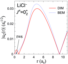
Figure 2: The modulus of the channel wave function ${u}_{j=0,\ell=0}$ near $r=0$ for the first excited $J^{\pi}=0_{2}^{+}$ state of LiCl^- calculated in DIM (solid line) and BEM (dotted line) with ${{\ell}_{max}=9}$. The charge separation ${s}$ of LiCl has been adjusted in both approaches to the experimental ground state energy in the limit ${{\ell}_{max}\rightarrow\infty}$.

For $\ell_{max}=9$ the ground state energy of the LiCl^- anion is reproduced by taking the charge separation $s_{\rm DIM}^{(9)}=0.336\,a_{0}$. To remove the dependence of results on $\ell_{max}$ in the DIM, the ground state energy of LiCl^- is extrapolated for $\ell_{max}\rightarrow\infty$, and the size of the charge separation $s$ is adjusted to reproduce the experimental binding energy. In this case, $s_{\rm DIM}^{(\infty)}=0.337\,a_{0}$. The matching radius was taken as $r_{m}=\,a_{0}$. This value was found to optimize the DIM procedure.

Anion spectra in the BEM depend sensitively on the cutoff parameter $k_{max}$ of the single-particle basis. However, as we shall see in Sec. VII, for a chosen value of $k_{max}$ they are practically independent of $\ell_{max}$. In this study, we have chosen $k_{max}=1.53\,a_{0}^{-1}$ for each partial wave in order to attain both a good numerical precision and approximately the same value of the dipole size parameter $s$ as in DI. In this case, $s_{\rm BEM}^{(9)}=s_{\rm BEM}^{(\infty)}=0.336\,a_{0}$. We have used complex contours with straight segments connecting points: $k_{1}=(0,0)$, $k_{2}=(0.15,-i0.04)$, $k_{3}=(1,0)$, and $k_{4}=k_{max}$ in units of $a_{0}^{-1}$. Each scattering contour has been discretized with 220 points. The precise form of the contour does not change results; since the applications carried out in this work pertain to bound states only, we could have used real scattering contours, i.e., the Newton completeness relation Michel et al. (2009); Newton (1982).

VII Numerical tests and benchmarking

Along with the asymptotic behavior of channel wave functions, treated approximately with the DIM and exactly within BEM, the Hamiltonian (2) cannot be identically represented in both approaches. Indeed, since the potential ${{V}_{\mu}(r)}$ (4) is not differentiable at ${r=s}$, it cannot be treated exactly in BEM because the channel wave functions expanded in the Berggren basis are analytic by construction. In practice, this translates into a node beyond ${r=s}$ in DIM channel wave functions, which is absent in BEM.

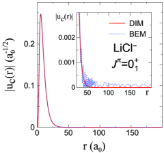
Figure 3: The modulus of the channel wave function ${u}_{j=0,\ell=0}$ for the $J^{\pi}=0_{1}^{+}$ ground state of LiCl^- calculated in DIM (solid line) and BEM (dotted line) with ${{\ell}_{max}=9}$. At large distances, spurious wiggles appear in BEM results (see the inset) due to basis truncation.

This is illustrated in Fig. 2 for a $(j=0,\ell=0)$ channel function corresponding to the first excited $J^{\pi}=0_{2}^{+}$ state of LiCl^-. It is to be noted, however, that beyond this point the channel wave functions calculated with both methods are very close and – as will be discussed later – this near-origin pathology has a very small impact on the total energy as the contribution from this region is small.

As discussed in Sec. IV.2, DIM is inadequate for states with very small energies, while BEM has been shown to be very precise in this case. On the other hand, for states with binding energies typically greater than $10^{-2}$ Ry, BEM yields channel wave functions that exhibit spurious low-amplitude oscillations. Figure 3 illustrates such wiggles in the tail of the channel wave function ${u}_{j=0,\ell=0}$ of the $J^{\pi}=0_{1}^{+}$ ground state of LiCl^-. For such well-bound states that quickly decay with $r$, the standard size of the Berggren basis (measured in terms of contour discretization points and $k_{max}$) is not sufficient. The DIM is thus preferable for such cases, as the asymptotic behavior of well-bound states is treated almost exactly (see Sec. IV.2).

The direct integration becomes numerically unstable when the channel orbital angular momentum becomes large, around ${\ell}_{c}=10$, even for the states with relatively large binding energies. In this case, the matrix of basis channel wave functions ${{u}^{0}_{b;c}(r_{m})}$ and ${{u}^{+}_{b;c}(r_{m})}$ and their derivatives, introduced in Sec. IV.1 in the context of matching conditions at $r=r_{m}$, is ill-conditioned and its eigenvector of zero eigenvalue becomes imprecise. This results in a discontinuity at ${r}_{m}$ and spurious occupation of channels with large orbital angular momentum ${\ell}_{c}>10$. This is illustrated in Fig. 4 for the $J^{\pi}=0_{1}^{+}$ ground state of LiCl^-. A a result, the energy and spatial extension of the electron cloud distribution of the CC eigenstate become incorrect.

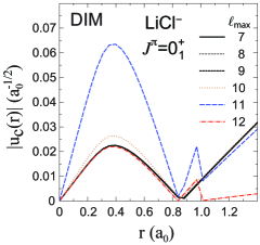
Figure 4: The modulus of the channel wave function ${u}_{j=0,\ell=0}$ for the $J^{\pi}=0_{1}^{+}$ ground state of LiCl^- calculated in DIM with several values of ${{\ell}_{max}}$. For ${{\ell}_{max}\geq 10}$, one may notice the development of a discontinuity at the matching point $r_{m}=a_{0}$. In such cases, the channel wave function becomes ill-conditioned, introducing serious errors in CC eigenenergy and eigenfunction.

The convergence of the LiCl^- ground state energy with respect to $\ell_{max}$ is shown in Fig. 5.

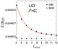
Figure 5: The dependence of the LiCl^- ground state energy on $\ell_{max}$ in DIM (dots) and BEM (triangles). The DIM results converge exponentially (red line). This allows us to determine the asymptotic value of energy at $\ell_{max}\rightarrow\infty$.

One may notice an exponential convergence of calculated DIM energies with $\ell_{max}$ for $6\leq\ell_{max}\leq 10$ and a clear deviation for $\ell\geq 11$, which is related to the discontinuity of channel wave functions for $\ell_{c}>10$. The energy calculated in BEM is perfectly stable with $\ell_{max}$.

The rapid converge of BEM with $\ell$ is due to $k_{max}$-truncation of the single-particle basis that suppresses contributions from large-$\ell$ configurations. This is illustrated in Fig. 6, which displays the average modulus of the off-diagonal matrix element of the channel-channel coupling in BEM:

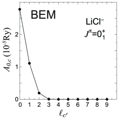
Figure 6: Average off-diagonal matrix element $A_{0,c}$ (39) of the channel-channel coupling in BEM between the channel $(j=0,\ell=0)$ and $c^{\prime}$ for the $J^{\pi}=0_{1}^{+}$ ground state of LiCl^-.

$$A_{c,c^{\prime}}=\frac{1}{N^{2}}\sum_{n,n^{\prime}}^{N}|\langle\Phi_{n^{\prime},c^{\prime}}|V|\Phi_{n,c}\rangle|$$ (39)

between the first channel $c=(j=0,\ell=0)$ and higher-$\ell$ channels $c^{\prime}$. Only the channels with $\ell_{c}\leq 5$ and $|\ell_{c}-\ell_{c^{\prime}}|\leq 3$ contribute significantly to the channel coupling matrix element. We checked that this is generally the case. Using the same truncation, the DIM yields numerically stable results. In this case, the energies of well-bound states ($|E|>10^{-2}$  Ry) agree in both methods.

The numerical instability of DIM at large $\ell_{max}$ leads to a collapse of calculated radii. Figure 7 shows the dependence of the ground state r.m.s. radius of LiCl^- on $\ell_{max}$.

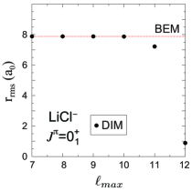
Figure 7: The dependence of the LiCl^- ground state r.m.s. radius on $\ell_{max}$ DIM (dots) and BEM (dotted line). The DIM results are stable up to $\ell_{max}=10$.

This result, together with discussion of Fig. 6, suggests that the BEM can provide practical guidance on the minimal number of channels in the CC approach.

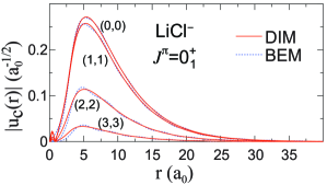
Figure 8: Most important channel wave functions $u_{c}(r)$ with $c=(j,\ell)$ for the $J^{\pi}=0_{1}^{+}$ ground state of LiCl^-, as calculated in DIM (solid line) and BEM (dashed line) with $\ell_{max}=9$.

In practical applications, spurious oscillations in BEM channel wave functions for well-bound states can be taken care of by extrapolating wave functions from the intermediate region of $r$, where they are reliably calculated, into the asymptotic region. This can be done by applying the analytical expression:

$${\tilde{u}}_{c}(r)\equiv\lim_{r\gg 0}u_{c}(r)=e^{ik_{c}r}\sum_{j=1}^{M}\frac{\alpha_{j}^{(c)}}{r^{j}},$$ (40)

where $k_{c}$ is the channel momentum and $\alpha_{j}^{(c)}$ are parameters to be determined by the fit. The precision of this procedure can be assessed by computing the norm of the eigenstate. Using this procedure, one obtains perfectly stable r.m.s. radii in BEM for different values of $\ell_{max}$, as can be seen in Fig. 7.

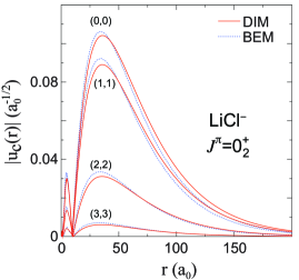
Figure 9: Similar to Fig. 8 but for the first excited $J^{\pi}=0_{2}^{+}$ state of LiCl^-.

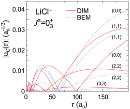
Figure 10: Similar to Fig. 8 but for the second excited $J^{\pi}=0_{3}^{+}$ state of LiCl^-.

Figures 8-10 compare the four most important channel wave functions $(\ell,j)$ of DIM and BEM corresponding to the three lowest $J_{i}^{\pi}=0_{i}^{+}$ eigenstates of LiCl^-. For the ground state, both approaches predict the same energy $E=-4.483\cdot 10^{-2}$ Ry and the channel functions are practically identical. For the first excited state, the agreement is still reasonable. Here, the energy in DIM is $E=-7.374\cdot 10^{-4}$ Ry while BEM gives slightly more binding: $E=-8.241\cdot 10^{-4}$ Ry. Consequently, the BEM wave functions decay faster than those computed with DIM. For a second excited $0_{3}^{+}$ state, both methods differ markedly. This state has a sub-threshold nature, with $E_{\rm DIM}=-7.051\cdot 10^{-6}$ Ry and $E_{\rm BEM}=-9.907\cdot 10^{-6}$ Ry. For this extremely diffused state, the direct integration method fails completely. This is manifested by the very different nodal structure of channel wave functions in DIM seen in Fig. 10.

A stringent test of the computational framework to describe dipolar molecules is provided by the analytic result ${\mu}_{cr}=0.639\,ea_{0}$ for the fixed dipole ($I\rightarrow\infty$) Lévy-Leblond (1967). To this end, we performed BEM calculations for a dipolar system at steadily decreasing moments of inertia Garrett (1971, 1980a). For each value of $I$, the dipolar anion energies have been calculated for 1080 values of $\mu$ in the interval $0.6\leq\mu\leq 3.0$. Only 170 energies satisfying the subthreshold condition $E<E_{lim}=-10^{-8}$ Ry were retained to minimize the numerical error. These energies correspond to an interval $\Delta\mu\simeq 0.377$ of the dipole moment. We checked, that in this energy interval, $\mu_{cr}$ can be obtained by using the expression

$$E(\mu)={(\mu+b)}^{\frac{a}{\mu}}{e}^{c}$$ (41)

to extrapolate the calculated energy down to $E=0$. One should stress however, that an excellent energy fit in the subthreshold region does not guarantee an excellent estimate of the critical dipole moment. The values of $\mu_{cr}$ extracted by this extrapolation procedure can be considered reliable only if $\Delta\mu$, which depends on the chosen precision $E_{lim}$, is close to the critical dipole moment. In the cases studied, this criterion is approximately satisfied only for the ground state and the first excited $0^{+}$ state. The critical dipole moments for these states in anions with the dipole length $s=4a_{0}$ are shown in Table 1 for various moments of inertia.

Table 1: Critical dipole moments for dipolar anions in the two lowest $0^{+}$ states calculated in this work (BEM) and in Ref. Garrett (1980a) for the charge separation $s=4a_{0}$ and different moments of inertia $I$. The analytic result at $I\rightarrow\infty$ Fermi and Teller (1947); Lévy-Leblond (1967) is ${\mu}_{cr}=0.639\,ea_{0}$.

$I(m_{e}a_{0}^{2})$	${\mu}_{cr}^{(0)}\,(e{a}_{0})$		${\mu}_{cr}^{(1)}\,(e{a}_{0})$
	BEM	Ref. Garrett (1980a)	BEM	Ref. Garrett (1980a)
${{10}^{4}}$	0.937	0.843	1.024	1.515
${{10}^{6}}$	0.674	0.750	0.633	1.145
${{10}^{8}}$	0.639	0.715	0.622	0.974
${{10}^{10}}$	0.639	—	0.622	—
${{10}^{15}}$	0.639	—	0.62	—

The agreement with the analytic limit is excellent for the ground state configuration, and is fairly good for the first excited 0⁺ state. This is very encouraging, considering the slow convergence with $I$ and various sources of numerical errors in the $E\rightarrow 0$ regime Garrett (1971).

VIII Results for spectra and radii of dipolar anions

Energies and r.m.s. radii of the lowest bound $0^{+}$ and $1^{-}$ states of LiI^-, LiCl^-, LiF^-, and LiH^- dipolar anions predicted in this study are listed in Table 2.

Table 2: Energies and r.m.s. radii for $0^{+}$ and $1^{-}$ bound states of selected dipolar anions obtained in DIM ($\ell_{max}=9$) and BEM. The parameters of the calculation are given in Sec. VI. The numbers in parentheses denote powers of 10.

Anion	state	$E$ (Ry)		$r_{\rm rms}\,({a}_{0})$
		DIM	BEM	DIM	BEM
LiI-	$0_{1}^{+}$	-5.079(-2)	-5.023(-2)	7.569(0)	7.620(0)
	$0_{2}^{+}$	-9.374(-4)	-1.037(-3)	5.112(1)	4.759(1)
	$0_{3}^{+}$	-1.502(-5)	-1.797(-5)	3.719(2)	3.308(2)
	$1_{1}^{-}$	-5.079(-2)	-4.995(-2)	7.569(0)	7.641(0)
	$1_{2}^{-}$	-9.291(-4)	-1.023(-3)	5.112(1)	4.886(1)
	$1_{3}^{-}$	-1.261(-7)	-1.099(-5)	3.423(3)	3.464(2)
LiCl-	$0_{1}^{+}$	-4.483(-2)	-4.483(-2)	7.885(0)	7.894(0)
	$0_{2}^{+}$	-7.374(-4)	-8.241(-4)	5.632(1)	5.017(1)
	$0_{3}^{+}$	-7.051(-6)	-9.907(-6)	5.124(2)	4.106(2)
	$1_{1}^{-}$	-4.482(-2)	-4.458(-2)	7.885(0)	7.915(0)
	$1_{2}^{-}$	-7.241(-4)	-8.067(-4)	5.633(1)	5.337(1)
	$1_{3}^{-}$	-3.062(-7)	-8.159(-7)	2.066(3)	8.831(2)
LiF-	$0_{1}^{+}$	-2.795(-2)	-2.983(-2)	9.117(0)	8.991(0)
	$0_{2}^{+}$	-3.022(-4)	-3.525(-4)	8.098(1)	7.501(1)
	$0_{3}^{+}$	—	-6.101(-8)	—	3.363(3)
	$1_{1}^{-}$	-2.793(-2)	-2.968(-2)	9.117(0)	9.010(0)
	$1_{2}^{-}$	-2.782(-4)	-3.277(-4)	8.124(1)	7.520(1)
LiH-	$0_{1}^{+}$	-2.149(-2)	-2.370(-2)	1.011(1)	9.698(0)
	$0_{2}^{+}$	-1.491(-4)	-1.922(-4)	1.058(2)	9.297(1)
	$1_{1}^{-}$	-2.142(-2)	-2.353(-2)	1.011(1)	9.717(0)
	$1_{2}^{-}$	-7.942(-5)	-1.231(-4)	1.146(2)	9.591(1)

One can see that for each total angular momentum $J^{\pi}$ there are at most three bound eigenstates in each system. The r.m.s. radius of an electron cloud shows a spectacular increase with decreasing the binding energy of the state. For the subthreshold states, such as $0_{3}^{+}$ and $1_{3}^{-}$, the radius is of the order of hundreds to thousands $a_{0}$.

Energy spectra and radii of dipolar anions do not change significantly in the limit $\ell_{max}\rightarrow\infty$. Usually, the extrapolated results for both $E$ and $r_{rms}$ agree very well with those in Table 2 ($\ell_{max}=9$). For instance, the extrapolated values for the $1_{2}^{+}$ state in LiH^- are $E=-7.931\cdot 10^{-5}$ Ry and $r_{\rm rms}=1.147\cdot 10^{2}\,a_{0}$.

The DIM and BEM results are generally consistent for both energy and radii though significant quantitative differences persist for excited, weakly-bound states of anions where the DIM is not expected to work. In the case of LiF^-, the BEM predicts the existence of the third $0_{3}^{+}$ state at an energy $-6.1\cdot 10^{-8}$  Ry, which is absent in DIM.

It is instructive to compare our DIM results with those found in Ref. Garrett (1982) using a similar approach. Table 3 lists energies of the lowest $0^{+}$ bound states of LiI^-, LiCl^-, LiF^-, and LiH^- dipolar anions obtained in both studies, and Table 4 shows the adopted values of dipole moments.

Table 3: Energies for $0^{+}$ bound states of selected dipolar anions obtained in DIM in this work ($\ell_{max}=9$) and in Ref. Garrett (1982). The numbers in parentheses denote powers of 10.

Anion	state	$E$ (Ry)
		This work	Ref. Garrett (1982)
LiI-	$0_{1}^{+}$	-5.079(-2)	-4.998(-2)
	$0_{2}^{+}$	-9.374(-4)	-1.022(-3)
	$0_{3}^{+}$	-1.502(-5)	-1.999(-5)
LiCl-	$0_{1}^{+}$	-4.483(-2)	-4.483(-2)
	$0_{2}^{+}$	-7.374(-4)	-7.497(-4)
	$0_{3}^{+}$	-7.051(-6)	-9.775(-6)
LiF-	$0_{1}^{+}$	-2.795(-2)	-2.793(-2)
	$0_{2}^{+}$	-3.022(-4)	-3.366(-4)
	$0_{3}^{+}$	—	-8.746(-7)
LiH-	$0_{1}^{+}$	-2.149(-2)	-2.352(-2)
	$0_{2}^{+}$	-1.491(-4)	-1.926(-4)

The two calculations agree reasonably well for the lowest-lying states; some difference stems from slightly different dipole moments used in Ref. Garrett (1982) and here. Indeed, while the charge separation in both studies was adjusted to reproduce the experimental ground state energy of LiCl^-, the fitted values of $s$ in both calculations are different: $s=0.3335~{}a_{0}$ in Ref. Garrett (1982) and $s_{\rm DIM}=0.336~{}a_{0}$ here.

The largest deviations, seen for weakly-bound states, can be traced back to the cutoff value of the electron orbital angular momentum when solving CC equations. In Ref. Garrett (1982), adopted $\ell_{max}$ was small, typically $\ell_{max}=4$ S. Ard, W. R. Garrett, R. N. Compton, L. Adamowicz, and S. G. Stepanian, Chem. Phys. Lett. 473, 223 () (2009), whereas it is fairly large, $\ell_{max}=9$, in our work. As seen in Fig. 5 and discussed in Sec. VII, energies of weakly-bound states obtained in DIM do converge slowly with $\ell_{max}$. Therefore, calculations employing low $\ell_{max}$ values cannot be useful when performing extrapolation $\ell_{max}\rightarrow\infty$.

Table 4: Dipole moments of selected dipolar anions adopted in this work and in Ref. Garrett (1982).

Anion	$\mu$ ($ea_{0}$)
	This work	Ref. Garrett (1982)
LiI-	2.911384272	2.911384272
LiCl-	2.805158089	2.793355179
LiF-	2.472316049	2.478610934
LiH-	2.313370205	2.321238811

IX Conclusions

In this study, we applied the theoretical open-system framework based on the Berggren ensemble to a problem of weakly-bound states of dipole-bound negative anions. The method has been benchmarked by using the traditional technique of direct integration of CC equations. While a fairly good agreement between the two methods has been found for well-bound states, the direct integration technique breaks down for weakly-bound states with energies $|E|<10^{-4}$ Ry, which is comparable with the rotational energy of the anion. For those subthreshold configurations, the Berggren expansion is an obvious tool of choice.

The inherent problem of the DIM is the lack of stability of results when the number of channels is increased. Indeed, the method breaks down when the channel orbital angular momentum becomes large; around $\ell_{c}=10$. This can be traced back to the applied matching condition. We demonstrated that this pathology is absent in BEM. Here, the rapid converge with $\ell$ is guaranteed by an effective softening of the interaction through the momentum cutoff $k_{max}$, which suppresses contributions from high-$\ell$ partial waves.

The future applications of BET will include the structure of quadrupole-bound anions Ferron et al. (2004); Desfrançois et al. (2004); Garrett (2008, 2012) and the continuum structure of anions, including the characterization of low-lying resonances.