Interplay of inter-chain interactions and exchange anisotropy:
Stability of multipolar states in quasi-1D quantum helimagnets

Abstract

We quantify the instability towards the formation of multipolar states in coupled spin-1/2 chain systems with a frustrating $J_{1}$-$J_{2}$ exchange, in parameter regimes that are of directly relevance to edge-shared cuprate spin-chain compounds. Three representative types of inter-chain coupling and the presence of uniaxial exchange anisotropy are considered. The magnetic phase diagrams are determined by Density Matrix Renormalization Group calculations and completed by exact analytic results for the nematic and dipolar phases. We establish that the residual couplings strongly affect the pitch of spiral states and their instability to multipolar phases. Our theoretical results bring to the fore novel candidate materials close to quantum nematic/triatic ordering.

In a system with frustrated magnetic interactions entirely new ground states (GS) can emerge from the ensuing competition. The geometric frustration of classical Ising spins on a pyrochlore lattice, for instance, results in the famous spin-ice state, the excitations of which are magnetic monopoles Castelnovo et al. (2008). In frustrated quantum magnets equally exotic states such as spin liquids, valence-bond crystals or nematic phases, can occur Lacroix et al. (2011). In quantum spin chain systems, in particular, the competition between short and longer-range magnetic couplings is a common source of frustration, a canonical example of which is the $J_{1}$-$J_{2}$ spin-1/2 chain Lacroix et al. (2011). Having antiferromagnetic (AFM) next nearest-neighbor (NNN) interactions ($J_{2}>0$), it is frustrated for any sign of the nearest-neighbor (NN) coupling ($J_{1}$). In the classical $J_{1}$-$J_{2}$ spin chain the competing interactions generate a helimagnetic state but in a single chain quantum fluctuations destroy the long-range helical order for any value of $J_{1}$. For sufficiently high magnetic field, for any value of $J_{1}$, the FM state takes over and the system’s magnons, its propagating spin-flips, become its exact single-particle excitations. The exchange parameters $J_{1}$ and $J_{2}$ determine the magnon dispersion and, in particular, the interaction between them. An AFM interaction leads to a repulsion between magnons, whereas a FM interaction results in an attraction, which favors the formation of magnon bound states. For a frustration ratio $\alpha$=$-J_{2}/J_{1}>0.367$ an interesting and intensely studied nematic state can occur, which may be thought of as a condensate of 2-magnon bound states Chubukov (1991); Kecke et al. (2007); Vekua et al. (2007); Hikihara et al. (2008); Sudan et al. (2009); Dmitriev and Krivnov (2009); Zhitomirsky and Tsunetsugu (2010); Svistov et al. (2011); Syromyatnikov (2012); Sizanov and Syromyatnikov (2013) characterized by a quadrupole spin order with a non-zero anomalous average $\langle\hat{S}_{i}^{+}\hat{S}_{j}^{+}\rangle$. For $1/4<\alpha<0.367$ also 3-, 4- and even higher magnon bound states can condense, resulting in a rich phase diagram with quite a number of exotic magnetic multipolar phases (MPPs).

These theoretical developments have stimulated an experimental quest to find multipolar condensates in quasi one-dimensional (1D) magnetic materials, in particular in spin $s=1/2$ systems consisting of edge-sharing copper-oxide chains, such as LiVCuO₄ (in cuprate notation $\equiv$LiCuVO₄ in traditional chemical notation)) Enderle et al. (2005); Büttgen et al. (2007, 2010); Hagiwara et al. (2011); Svistov et al. (2011), Li₂ZrCuO₄ Drechsler et al. (2007); Schmitt et al. (2009), Ca₂Y₂Cu₅O₁₀ Matsuda et al. (2001); Kuzian et al. (2012), PbCuSO₄(OH)₂ Wolter et al. (2012); Willenberg et al. (2012), Rb₂Cu₂Mo₃O₁₂ Hase et al. (2004) and Li₂CuO₂ Lorenz et al. (2009); Nishimoto et al. (2011). In these systems $J_{1}$ is intrinsically FM and $J_{2}$ can be of comparable strength, but AFM. In real 3D materials, however, a magnetic inter-chain (IC) interaction is unavoidably present. Due to the fragility of purely 1D bound-states, AFM IC interactions can pose a very relevant perturbation to a multipolar state, even when the coupling strength is (very) small Nishimoto et al. (2011). To establish the consequences of this key ingredient for the stability of MPPs we consider here the three most common types of IC couplings $J^{\rm IC}$ that are encountered in the quasi-1D edge-shared cuprates mentioned above (one perpendicular IC coupling and two different types of skew ones, see Fig. 1) and determine the boundaries of the magnetic phase diagram numerically by Density Matrix Renormalization Group (DMRG) calculations and analytically by hard-core boson (HCB) Kuzian and Drechsler (2007); SM ; Nishimoto et al. (2011); Nishimoto et al. (2012a, b)) and spin-wave (SW) Kuzian et al. (2012) approaches. On top of this we consider also the presence of a uniaxial exchange anisotropy $\Delta-1$ for the NN coupling along the chains, which is the leading anisotropy term in edge-shared chain cuprates Tornow et al. (1999); Yushankhai and Hayn (1999); Kataev et al. (2001); Heidrich-Meisner et al. (2009). We show that the stability of MPPs is strongly affected by the strength of the AFM IC couplings and depends on the precise type (geometry) of this coupling, which may also largely affect the pitch of the spiral state. A small easy-axis exchange anisotropy, however, enhances the stability of MPPs dramatically, also in the presence of IC coupling, since it enhances the attraction between magnons. From the material’s viewpoint, our theoretical results bring to the fore linarite, PbCuSO₄(OH)₂, as a promising candidate compound with a triatic MPP, which can be stabilized by its sizable exchange anisotropy and confirm the closeness of LiVCuO₄ to quantum nematicity.

The relevant Hamiltonian $H=H_{1D}+H_{IC}$ encompasses the frustrating magnetic interactions along the 1D chain in the presence of an external magnetic field $h$ and a small uniaxial exchange anisotropy $\Delta-1$

$$H_{1D} = \sum_{n,i}\left[-{\bf S}_{n,i}\cdot{\bf S}_{n,i+1}+\alpha{\bf S}_{n,i}\cdot{\bf S}_{n,i+2}\right]$$ (1)

$$- \sum_{n,i}\left[(\Delta-1)S_{n,i}^{z}S_{n,i+1}^{z}+hS_{n,i}^{z}\right],$$

where $n$ labels the chain and $i$ the position of the spins along the chain. Neighboring chains $n$ and $m$ interact via

$$H_{\rm IC}=\sum_{\langle nm\rangle,r}J^{\rm IC}_{r}{\bf S}_{n,i}\cdot{\bf S}_{m,i+r},$$ (2)

where $r=0$ corresponds to a perpendicular IC coupling and $r=1,2$ refer to skew IC couplings, see Fig. 1. We use $|J_{1}|$ as the energy unit of all coupling constants in $H$.

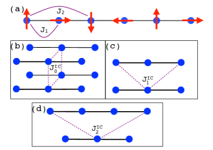
Figure 1: (a) Competing NN and NNN exchange $J_{1}$ and $J_{2}$, respectively, along a chain. Coupling between different chains: (b) perpendicular coupling $J^{\rm IC}_{0}$ (e.g., LiVCuO₄), (c) skew (diagonal) coupling $J^{IC}_{1}$ (e.g., PbCuSO₄(OH)₂) and (d) skew NNN coupling between shifted chains $J^{\rm IC}_{2}$ (e.g., Li₂CuO₂). The effect of $J^{\rm IC}$ is considered in both 2D and 3D.

To determine the nature of the magnetic GS and its dependence on the frustration $\alpha$, the different types of IC exchange $J^{\rm IC}$ and the exchange anisotropy $\Delta-1$, we employed the DMRG method White (1992) with periodic boundary conditions (PBC) for all directions. This method is not restricted to purely 1D and can also be used for 2D  Nishimoto et al. (2010); Stoudenmire and White (2012) and 3D Nishimoto et al. (2011); Nishimoto et al. (2012b) systems, although the system size is limited, e.g., up to about $\sqrt{N}\times\sqrt{N}\times L=\sqrt{10}\times\sqrt{10}\times 50$ for spin Hamiltonians. We kept $p\approx 800-5000$ density-matrix eigenstates in the renormalization procedure. About $100-300$ sweeps are necessary to obtain the GS energy within a convergence of $10^{-7}J_{1}$ for each $p$ value. All calculated quantities were extrapolated to $p\to\infty$ and the maximum error in the GS energy is estimated as $\Delta E/J_{1}\sim 10^{-4}$, while the discarded weight is less than $1\times 10^{-6}$. Under the PBC, a uniform distribution of $\left\langle S^{z}_{i}\right\rangle$ may give an indication to examine the accuracy of DMRG calculations for spin systems. Typically, $\left\langle S^{z}\right\rangle-S_{\rm tot}^{z}/(NL)$ is less than $1\times 10^{-3}$ in our calculations. Note that for high-spin states [$S_{\rm tot}^{z}\gtrsim(NL-10)/2)$] the GS energy can be obtained with an accuracy of $\Delta E/J_{1}<10^{-12}$ by carrying out several thousands sweeps even with $p\approx 100-800$.

We considered systems with different lengths: $L=16-64$ ($24-96$) for 3D (2D) and adopted power laws to perform a finite-size-scaling analysis. From this we obtained the saturation field $h_{s}$ in the thermodynamic limit $L\to\infty$. As a result, we obtain $h_{s}$ with high accuracy. In addition to DMRG we have also applied an analytic HCB-approach and the linear SW approach Kuzian and Drechsler (2007); SM to provide exact results for the nematic and dipolar phases. In addition, some of the calculated magnetization curves have been cross-checked by exact diagonalization.

The simplest case, relevant for, e.g., LiVCuO₄ and Li(Na)Cu₂O₂, is the situation of unshifted neighboring chains and a perpendicular inter-chain exchange $J^{\rm IC}_{0}$, see Fig. 1a. In this case spirals on NN chains are only weakly affected by an AFM IC coupling Zinke et al. (2009) – on a classical level the pitch of the incommensurate (INC) spiral state is not affected by $J^{\rm IC}_{0}$. This is in stark contrast to the effect of skew AFM $J^{\rm IC}_{1}$ and $J^{\rm IC}_{2}$, which can strongly reduce the pitch.

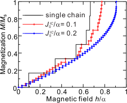
Figure 2: Magnetization vs. magnetic field for a 2D arrangement of four chains with $N=24$ sites each, with a perpendicular IC coupling $J^{\rm IC}_{0}$ (cf. Fig. 1b), $\alpha=1/2$ and $\Delta=1$.

A typical magnetization curve for $\alpha$=0.5 and $\Delta=1$, for a nematic phase, is shown in Fig. 2. The height of the magnetization steps $\Delta S^{z}$=2 when $J^{\rm IC}_{0}/\alpha$=0.1, is the direct signature for 2-magnon bound states. A larger value of the IC coupling suppressed these bound states, as is clear from the magnetization curve for $J^{IC}_{0}/\alpha$=0.2 where the steps correspond to $\Delta S^{z}$=1. So in the isotropic case, where $\Delta=1$, a rather weak critical IC of a few percent destroys the nematic phase in favor of the usual conical ordering. The critical value for $J^{IC}_{0}/(\alpha=0.5)$ amounts 0.188/0.088 in 2D/3D, respectively. The full phase diagram rem is shown in Fig. 3, where the phase boundaries are extracted from the kinks in the calculated saturation field $h_{s}$ as a function of $J^{IC}_{0}$, as shown in Fig. 3(a-c). Clearly, the 3- , 4- , and higher multimagnon MPPs are even stronger affected by the IC interaction.

Allowing for a finite uniaxial exchange anisotropy $\Delta-1$, the leading-order anisotropy that is of immediate relevance to quasi-1D cuprates Tornow et al. (1999); Yushankhai and Hayn (1999) affects the stability of the MPP substantially. Fig. 3 shows that for $\alpha=1/2$ an anisotropy $\Delta-1$ of just 0.1 increases the critical IC coupling by a factor of $\sim$1.6, and thus significantly enhances their stability region.

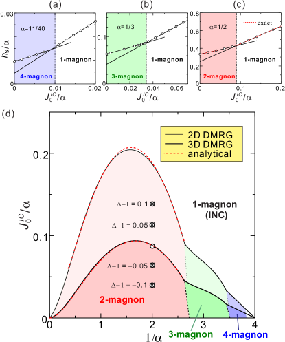
Figure 3: (a-c) Saturation field $h_{s}$ as a function of the perpendicular IC coupling $J^{\rm IC}_{0}$ (cf. Fig. 1b) and $\Delta=1$. (d) Phase diagram with critical IC coupling in 3D and 2D (thin line). Phase boundaries are extracted from the kinks in the $h_{s}$ as in (a-c). Red dashed lines: analytical HCB results [Eq. (S54)]. Symbols: the dependence of the critical $J^{\rm IC}_{0}$ on the uniaxial exchange anisotropy $\Delta-1$ in 3D for $\alpha=0.5$, where $\circ$/$\times$ correspond to the DMRG/analytical HCB results, respectively.

Our analytical approach to calculate the phase boundary between the 1- and 2-magnon instabilities relies on first deriving the saturation fields of these two instabilities: $h_{s,1}$ and $h_{s,2}$ respectively. Requiring them to be equal then renders the equation for the critical IC coupling as a function of anisotropy and frustration parameters. The saturation field $h_{s,1}$ of the INC phase on the 1-magnon side is exact already within SW theory:

$$h_{s,1}=\frac{(4\alpha-1)^{2}}{8\alpha}+\frac{N_{\rm IC}}{2}(J^{\rm IC}_{0}+|J^{\rm IC}_{0}|)-(\Delta-1),$$ (3)

where $N_{\rm IC}$ denotes the number of IC neighbors (i.e. for $J^{\rm IC}_{0}$ in 3D and 2D, $N_{\rm IC}=4$ and 2, respectively). In the Supplementary Material this expression has been further generalized to include next NN and IC exchange anisotropies SM . Therein we have shown also that the critical value of $J_{0}^{\rm IC}$ of perpendicular IC depends only on $\Delta$, $\alpha$, and $N_{\rm IC}$. For the nematic phase we obtained exact values of $h_{s}$ using the HCB-approachKuzian and Drechsler (2007); SM . The HCB values are in full accord with the DMRG results. In the limit $J^{\rm IC}\ll 1$ we arrive at the analytical expansion $h_{\mbox{\tiny s,2}}\simeq h_{\mbox{\tiny s}}^{\rm 1D}+\eta_{2}(J^{\rm IC})^{2}+\eta_{4}(J^{\rm IC})^{4},$ which is approximate but accurate enough for our present purposes and where $h_{s}^{\rm 1D}=-\Delta+2\alpha+\Delta^{2}/(2\Delta+2\alpha)$ Kuzian and Drechsler (2007), and $2\eta_{2}(\alpha,\Delta)=N_{IC}(\Delta+\alpha)(3\alpha^{2}+3\alpha\Delta+\Delta^{2})/[\Delta(\Delta+2\alpha)]^{2}\approx N_{IC}\left(5/6+3\alpha/4\right)$, when $\Delta\sim 1$. The expression for the next, quartic term $\eta_{4}$ is provided in Ref. SM, . Comparing the expressions for $h_{s,1}$ and $h_{s,2}$ one notices the presence of nonlinear IC terms and a two times smaller linear term in the nematic phase as compared to the usual 1-magnon phase. The solution of the equation $h_{s,2}=h_{s,1}$ gives analytical expressions for the critical IC interaction $J^{\rm IC}_{\rm 0,cr}$. Keeping only the linear term in the expression for $h_{s,2}$, we find (cf. Eq. (51) in Ref. Syromyatnikov, 2012) $|J^{\rm IC}_{\rm 0,cr1}|=(4\alpha\Delta^{2}-\Delta-\alpha)/[4\alpha\left(\Delta+\alpha\right)N_{\rm IC}]$ and including the quadratic term SM , we obtain

$$|J^{IC}_{0,cr2}|=\frac{1}{4\eta_{2}}\left(N_{IC}-\sqrt{N_{IC}^{2}-8\eta_{2}N_{IC}|J^{IC}_{0,cr1}|}\right).$$ (4)

A comparison of the numerical DMRG results in Fig. 3 (cf. Fig. 6 of Ref. Ueda and Totsuka, 2009) shows that Eq. (S54) is very accurate for 3D systems and works well for 2D ones, too.

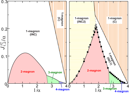
Figure 4: Phase diagram for MPP swith skew (diagonal) IC coupling $J^{\rm IC}_{1}$ (left) and $J^{\rm IC}_{2}$ (right) in 3D.

The phase diagram for the situation of the two other, skew types of IC interaction, $J^{\rm IC}_{1}$ and $J^{\rm IC}_{2}$ (see Fig. 1c and d) are shown in Fig. 4. An inspection of the phase diagrams reveals that the maximal value for the critical $J^{\rm IC}$ always occurs in the nematic phase at $\alpha$ slightly below 1, i.e. in the region of maximal in-chain frustration and quantum behavior Kuzian and Drechsler (2007); Nishimoto et al. (2012a). For the situation of perpendicular coupling this can be understood already in linear approximation, where $j_{\rm cr,1}$ is proportional to the difference of 1- and 2-magnon critical fields of an isolated chain $j_{\rm cr,1}=2(h_{\mbox{\tiny s}}^{\mbox{\tiny 1D}}-h_{s,1}^{\mbox{\tiny 1D}})/N_{\rm IC}$. Near the critical point ($\alpha\gtrsim$ 1/4) and for almost decoupled Heisenberg chains the saturation field tends to the simple 1-magnon value and additional quantum effects vanish.

Having investigated theoretically in general how the competition between frustration, different types of IC coupling and exchange anisotropy plays out, we now apply these insights to identify candidate materials potentially displaying a quantum MPP. Li₂CuO₂ is near the critical point, having $\alpha\approx 0.33$ and a rather small $\Delta-1\approx 0.01$ Lorenz et al. (2009). Its IC coupling $J^{\rm IC}_{2}$, however, is strong enough to even destabilize the spiral state and drives the chains FM. Also Li₂ZrCuO₄ is close to the critical point ($\alpha\approx 0.3$ Drechsler et al. (2007)) but in this case as well for any realistic IC interaction and reasonable value for $\Delta$, all higher MPP are unstable. The compounds Li(Na)Cu₂O₂ are away from the detrimental critical point but their IC coupling is too large ($J^{IC}\sim 0.5$ to 1 Gippius et al. (2004); Masuda et al. (2005); Drechsler et al. (2006)) to establish a nematic phase for the estimated, moderate, values of $\Delta$ Mihály et al. (2006).

Instead LiVCuO₄ is a good material for a nematic phase, having a coupling between the chains that is characterized by a very weak $J^{\rm IC}_{0}$, which manifests itself in strong quantum fluctuations evidenced by a small ordered magnetic moment ($0.3\mu_{\mbox{\tiny B}}$) at low temperature and the observation of a 2-spinon continuum in inelastic neutron scattering Enderle et al. (2010). The weak $J^{\rm IC}$ is also in accord with the fact that its saturation field is close to the value of the uncoupled 1D-chain given by $h_{s}^{\rm 1D}$ Drechsler et al. (2011). In addition, the estimated $\alpha\approx 0.75$ Nishimoto et al. (2012a); Drechsler et al. (2011), near the maximum of the critical $J^{\rm IC}_{0,{\rm cr}}(1/\alpha)$-curve is almost optimal for a nematic phase to survive (see Fig. 3).

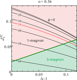
Figure 5: Phase diagram and pitch (contour lines) as a function of the diagonal IC coupling $J^{\rm IC}_{1}$ (in units of $|J_{1}|$) and the uniaxial exchange anisotropy $\Delta-1$ for $\alpha=0.36$, as is relevant for linarite, PbCuSO₄(OH)₂. The red contour line corresponds to the experimental value of the pitch, 34^∘.

A very interesting case is provided by the natural mineral linarite, PbCuSO₄(OH)₂, which consists of neutral edge-shared Cu(OH)₂-chains surrounded by Pb²⁺ and [SO₄]^-2 ions and has $\alpha\approx 0.36$ Wolter et al. (2012). Below 2.7 K a spiral state with a pitch of 34^∘ sets in Yasui et al. (2011); Willenberg et al. (2012). A perpendicular $J^{\rm IC}_{0}$ barely affects the pitch of the spiral, in sharp contrast to skew IC coupling $J^{\rm IC}_{1}$. We have considered this situation theoretically in more detail and calculated the phase diagram as a function of $\Delta-1$ and $J^{\rm IC}_{1}$, see Fig. 5. For the given value of $\alpha$ a small $J^{IC}_{1}$ and $\Delta-1$ are enough to reduce the pitch from about 60^∘ to the experimental value of 34^∘. The experimental pitch strongly restricts the possible values for $J^{\rm IC}_{1}$ and $\Delta-1$ (see the red line in Fig. 5 ). An additional piece of information is the experimental value of the saturation field of 11 T – the 1D saturation field gives in this case about 5 T – which indicates a reduced value of $J^{\rm IC}_{1}$, renormalized by a sizable $\Delta-1$, placing the system close to the triatic, 3-magnon region of the phase diagram in Fig. 5.

In this context experimental studies under chemical or physical pressure are of great interest, since these can significantly change the IC coupling. When applying hydrostatic pressure one expects an increase of the IC coupling and thereby a weakening and possibly disappearance of the MPPs in the mentioned two candidate materials. Vice versa, growing isomorphic crystals with larger isovalent cations, i.e. substituting e.g. Li or Na by Na, Rb, or Cs, respectively, is expected to lead to candidate MPP materials due to a decrease of IC couplings. If possible to synthesize one expects e.g. for Cs(Rb)Cu₂O₂ and Na(Rb)₂ZrCuO₄ an increased stability of the nematic and triatic phase, respectively. Preparing strained epitaxial thin films from candidate materials will cause similar effects, where a tuning of the strain can change the IC in different directions.

We have, in summary, demonstrated the crucial role of different types of antiferromagnetic inter-chain interactions and the uniaxial exchange anisotropy in frustrated quasi-1D helimagnets. The rich and exotic physics of multipolar phases recently predicted for single chains is very sensitive to the strength and type and these additional and unavoidable interactions. Unfortunately, this prevents a realization of multipolar phases in most presently known spin-chain materials. But we find at least two notable exceptions: LiVCuO₄, where a nematic phase is expected, and linarite, PbCuSO₄(OH)₂, which according to our present calculations is in the close vicinity of a triatic instability. In addition we proposed several new material systems as potential candidates with magnetic multipolar ground states and point out the large experimental potential of tuning the interchain interactions by pressure and strain.

We thank the DFG [grants DR269/3-1 (S-LD, SN), RI615/16-1 (JR)] for financial support and H. Rosner, A. Wolter, and M. Schaeper for discussions on linarite.

At high magnetic fields, the Hamiltonian of coupled frustrated spin-1/2 chains with the ferro- antiferromagnetic $J_{1}$-$J_{2}$ XXZ-Heisenberg model reads

$$\hat{H} = \hat{H}_{1D}+\hat{H}_{ic}\quad,$$ (S1)

$$\hat{H}_{1D} = \sum_{\mathbf{m}}\left[\frac{1}{2}\sum_{\mathbf{r}}J_{\mathbf{r}}\left(\Delta_{\mathbf{r}}\hat{S}_{\mathbf{m}}^{z}\hat{S}_{\mathbf{m}+\mathbf{r}}^{z}+\hat{S}_{\mathbf{m}}^{+}\hat{S}_{\mathbf{m}+\mathbf{r}}^{-}\right)\right.$$ (S3)

$$\left.-\mu\mathcal{H}\hat{S}_{\mathbf{m}}^{z}\right]\ ,$$

$$\hat{H}_{ic} = \frac{1}{2}\sum_{\mathbf{f}}J_{\mathbf{f}}\left[\Delta_{\mathbf{f}}\hat{S}_{\mathbf{m}}^{z}\hat{S}_{\mathbf{m}+\mathbf{f}}^{z}+\hat{S}_{\mathbf{m}}^{+}\hat{S}_{\mathbf{m}+\mathbf{f}}^{-}\right]\ ,$$ (S4)

where $\mathbf{m}$ enumerates the lattice sites, ls $\mathbf{r}=\pm n\mathbf{a},\>n=1,2$ determines the NN sites within the chain, and $\mathbf{a}$ is the lattice vector along the chain. The vector $\mathbf{f}$ connects sites at different chains. We restrict ourself to the case of uniaxial exchange anisotropy and the magnetic field directed along that axis, $\mu\equiv g\mu_{\mbox{\tiny B}}$.

In terms of hard-core boson operators $b$, defined by

$$\begin{array}[]{rcl}\hat{S}^{+}\equiv b,\ \hat{S}^{-}\equiv b^{\dagger},&&\hat{S}^{z}\equiv\frac{1}{2}-\hat{n},\\ &&\hat{n}_{\mathbf{m}}=b_{\mathbf{m}}^{\dagger}b_{\mathbf{m}}=0,1,\\ \left\{b_{\mathbf{m}},b_{\mathbf{m}}^{\dagger}\right\}=1,&&\left[b_{\mathbf{m}},b_{\mathbf{m}^{\prime}}^{\dagger}\right]=0,\ \mathbf{m}\neq\mathbf{m}^{\prime},\\ b_{\mathbf{m}}^{\dagger}|FM\rangle&\equiv&b_{\mathbf{m}}^{\dagger}|\cdots\uparrow\uparrow\uparrow_{\mathbf{m}}\uparrow\uparrow\uparrow\cdots\rangle\\ &=&|\cdots\uparrow\uparrow\downarrow_{\mathbf{m}}\uparrow\uparrow\uparrow\cdots\rangle,\\ \left(b_{\mathbf{m}}^{\dagger}\right)^{2}&=&\left(b_{\mathbf{m}}\right)^{2}=0,\end{array}$$ (S5)

the Hamiltonian (S1) becomes

$$\hat{H} = \hat{H}_{0}+\hat{H}_{int},$$ (S6)

$$\hat{H}_{0} = \omega_{0}\sum_{\mathbf{m}}\hat{n}_{\mathbf{m}}+\frac{1}{2}\sum_{\mathbf{m,R}}J_{\mathbf{R}}b_{\mathbf{m}}^{\dagger}b_{\mathbf{m+R}},$$ (S7)

$$\hat{H}_{int} = \frac{1}{2}\sum_{\mathbf{m,R}}J_{\mathbf{R}}\Delta_{\mathbf{R}}\hat{n}_{\mathbf{m}}\hat{n}_{\mathbf{m+R}},$$ (S8)

where $\omega_{0}\equiv\mu\mathcal{H}-\frac{1}{2}\sum_{\mathbf{R}}J_{\mathbf{R}}\Delta_{\mathbf{R}}$, $\mathbf{R}=\mathbf{r,f}$.

The $n$-particle excitation spectra are given by the singularities of the corresponding retarded Green’s functions (GF)

$$\langle\langle\hat{X}|\hat{Y}\rangle\rangle \equiv -\imath\int_{t^{\prime}}^{\infty}\!\!dte^{i\omega(t-t^{\prime})}\left\langle\left[\hat{X}(t),\hat{Y}(t^{\prime})\right]\right\rangle,$$ (S9)

$$\omega\langle\langle\hat{X}|\hat{Y}\rangle\rangle = \left\langle\left[\hat{X},\hat{Y}\right]\right\rangle+\langle\langle\left[\hat{X},\hat{H}\right]|\hat{Y}\rangle\rangle.$$ (S10)

A negative value of the excitation energy signals an instability of the ground state, which is given by the fully polarized state achieved for a magnetic field above the saturation field $\mathcal{H}>\mathcal{H}_{s}$.

The equation of motion for the two-magnon operator

$$\begin{array}[]{rll}\hat{A}_{\mathbf{k,l}}&=&\frac{1}{\sqrt{N}}\sum_{\mathbf{m}}\mathrm{e}^{-\imath\mathbf{k}(\mathbf{m}+\mathbf{l}/2)}b_{\mathbf{m}}b_{\mathbf{m+l}}=\hat{A}_{\mathbf{k,-l}},\end{array}$$ (S11)

reads

$$\begin{array}[]{lll}\left[\hat{A}_{\mathbf{k,l}},\hat{H}\right]&=&\left(2\omega_{0}+\sum_{\mathbf{R}}J_{\mathbf{R}}\Delta_{\mathbf{R}}\delta_{\mathbf{l,R}}\right)\hat{A}_{\mathbf{k,l}}\\ &+&\left(1-\delta_{\mathbf{l,0}}\right)\sum_{\mathbf{R}}J_{\mathbf{R}}\cos\frac{\mathbf{kR}}{2}\hat{A}_{\mathbf{k,l+R}},\end{array}$$ (S12)

where $\mathbf{k}$ being the total quasi-momentum of the magnon pair, $N=N_{\perp}N_{x}$ is the number of sites, $N_{\perp}$ is the number of chains, and $N_{x}$ denotes the number of sites in the chain.

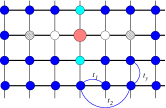
Figure S1: Cartoon of the effective impurity problem given by the Hamiltonian (S13), which describes the internal motion of a magnon pair with the total quasi-momentum $\mathbf{k}$. The pink, open, shaded and cyan circles depict the impurities with $\varepsilon_{\mathbf{m}}=\infty,J_{1}\Delta_{1},J_{2}\Delta_{2},J_{\perp}\Delta_{\perp}$ respectively, $\bullet$ : the regular sites of the lattice, arcs: the $\mathbf{k}$-dependent hoppings.

As usual, the exclusion of the center of mass motion reduces the problem of an interacting pair particles to a one-particle problem of motion in an effective potential well (EPW). In our case it corresponds to an impurity problem in a tight-binding Hamiltonian Kuzian and Drechsler (2007) (see Fig. S1)

$$\hat{H}_{tb}(\mathbf{k}) = \hat{T}(\mathbf{k})+\hat{V},$$ (S13)

$$\hat{T}(\mathbf{k}) = 2\omega_{0}\sum_{\mathbf{m}}\left|\mathbf{m}\right\rangle\left\langle\mathbf{m}\right|$$ (S15)

$$+\sum_{\mathbf{m,R}}\left|\mathbf{m+R}\right\rangle t_{\mathbf{R}}(\mathbf{k})\left\langle\mathbf{R}\right|,$$

$$\hat{V} = \sum_{\mathbf{m}^{\prime}}\left|\mathbf{m}^{\prime}\right\rangle\varepsilon_{\mathbf{m}^{\prime}}\left\langle\mathbf{m}^{\prime}\right|,$$ (S16)

where

$$t_{\mathbf{R}}(\mathbf{k}) = J_{\mathbf{R}}\cos\frac{\mathbf{kR}}{2},$$ (S17)

$$\mathbf{m}^{\prime}=\mathbf{0,r,f} \varepsilon_{\mathbf{0}}=\infty,\ \varepsilon_{\mathbf{R}}=J_{\mathbf{R}}\Delta_{\mathbf{R}}.$$ (S18)

The Hamiltonian depends on the total pair momentum.

The two-magnon GF reads

$$G_{\mathbf{l,n}}(\mathbf{k},\omega) = \left\langle\left\langle A_{\mathbf{k,l}}|A_{\mathbf{k,n}}^{\dagger}\right\rangle\right\rangle,$$ (S19)

$$= \left\langle\phi_{\mathbf{l}}\right|\left(\omega-\hat{H}_{tb}\right)^{-1}\left|\phi_{\mathbf{n}}\right\rangle$$ (S20)

with $\left|\phi_{\mathbf{l}}\right\rangle=\left(\left|\mathbf{l}\right\rangle+\left|-\mathbf{l}\right\rangle\right)/\sqrt{2}$. The GF is analytic everywhere in the complex energy plane but may have singularities on the real axis: branch cuts and isolated poles. The branch cuts correspond to the continuum spectrum of unbounded motion of the effective particle, which in its turn correspond to the two-particle continuum in the pair motion. The poles correspond to the energies of localized impurity states, which are bound states for the pair when the energies lie below the continuum or anti-bound states in the opposite case. It is clear from Eqs. (S13)-(S18) that bound states are possible only when some $\varepsilon_{\mathbf{R}}$ are negative, i.e. for FM $J_{\mathbf{R}}<0$. The bound state energy and the continuum boundaries depend on the total momentum of the pair $\mathbf{k}$. If the bound state energy minimum lies below the lowest continuum energy (that may occur at different $\mathbf{k}$-values), the bound pairs will condense at magnetic fields just below the saturation field, the gas of pairs being the nematic state of the magnetic systemChubukov (1991); Syromyatnikov (2012).

When all $J_{\mathbf{R}}$ are positive, like in AFM-AFM $J_{1}$-$J_{2}$ model, only anti-bound states occur at energies higher the two-particle continuum. In this case only the one-magnon condensation occurs below the saturation field.

We will use the identity

$$\hat{G}=\hat{g}+\hat{g}\hat{V}\hat{G}\ ,$$ (S21)

for the solution in the real space of the impurity problem given by Eqs. (S13)-(S20) (see Fig. S1). In Eq. (S21), $\hat{g}\equiv\left(\omega-\hat{T}\right)^{-1}$ is the resolvent operator for the periodic part, and $\hat{G}\equiv\left(\omega-\hat{H}_{tb}\right)^{-1}$ is the resolvent for the impurity problem. According to Ref. Economou, 2006, we may solve the problem step by step. Starting from the GF of a free particle, which in the matrix form reads

$$g_{\mathbf{l,n}} = g_{\mathbf{l-n}}(\mathbf{k},\omega)$$ (S22)

$$= \frac{1}{N}\sum_{\mathbf{q}}\frac{\cos\mathbf{q}(\mathbf{l-n})}{\omega-\left(\omega_{\mathbf{k}/2+\mathbf{q}}^{SW}+\omega_{\mathbf{k}/2-\mathbf{q}}^{SW}\right)},$$ (S23)

$$\omega_{\mathbf{q}}^{SW} = \omega_{0}+\frac{1}{2}\sum_{\mathbf{R}}J_{\mathbf{R}}\mathrm{e}^{\imath\mathbf{qR}},$$ (S24)

we add the impurity at the origin. Its infinite potential reflects the impossibility to have two particles on the same site (S5)

$$g_{\mathbf{l,n}}^{(\mathbf{0})} = g_{\mathbf{l,n}}+g_{\mathbf{l\mathbf{,0}}}\varepsilon_{\mathbf{0}}g_{\mathbf{0,n}}^{(\mathbf{0})},$$

$$g_{\mathbf{l,n}}^{(\mathbf{0})} = g_{\mathbf{l,n}}+\frac{g_{\mathbf{l,0}}\varepsilon_{\mathbf{0}}g_{\mathbf{0,n}}}{1-\varepsilon_{\mathbf{0}}g_{\mathbf{0,0}}}\rightarrow g_{\mathbf{l,n}}-\frac{g_{l\mathbf{,0}}g_{\mathbf{0,n}}}{g_{\mathbf{0,0}}}.$$ (S25)

Next, we add an impurity at the site $\mathbf{i}$ and express the GF via $\hat{g}^{(\mathbf{0})}$

$$g_{\mathbf{l,n}}^{(i)}=g_{\mathbf{l,n}}^{(\mathbf{0})}+\frac{g_{\mathbf{l,i}}^{(\mathbf{0})}\varepsilon_{\mathbf{i}}g_{\mathbf{i,n}}^{(\mathbf{0})}}{1-\varepsilon_{\mathbf{i}}g_{\mathbf{i,i}}^{(\mathbf{0})}},$$

and so on, the GF of the system with $r$ impurities is expressed via the GF of the system with $r-1$ impurities

$$g_{\mathbf{l,n}}^{(r)}=g_{\mathbf{l,n}}^{(r-1)}+\frac{g_{\mathbf{l,r}}^{(r-1)}\varepsilon_{\mathbf{r}}g_{\mathbf{r,n}}^{(r-1)}}{1-\varepsilon_{\mathbf{r}}g_{\mathbf{r,r}}^{(r-1)}}.$$ (S26)

Thus, in principle, we may take into account any number of in-chain and inter-chain exchange couplings (IC) and obtain $G_{\mathbf{l,n}}(\mathbf{k},\omega)$ (S19). The explicit expression for the GF $G_{1,1}(k,\omega)$ for the 1D $J_{1}$-$J_{2}$ model (S3) has been given in Ref. Kuzian and Drechsler, 2007. It’s spectral density is plotted in Fig. S2.

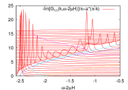
Figure S2: The spectral density of the two-particle Green’s function for an isolated chain. 1D case, i.e. $J_{1}$=-1, $J_{2}$=1, $J_{\perp}$=0. Cyan and magenta thin lines shows the lower boundary of the 2-magnon continuum.

The sharp $\mathbf{k}$-dependent peaks below the two-particle continuum corresponds to bound pairs of magnons.

At higher dimensions, the role of the inter-chain interaction (S4) is twofold. First, the periodic part of the effective Hamiltonian (S15) becomes D-dimensional. This changes $\hat{g}$ from Eq. (S22) via the change of $\omega_{\mathbf{q}}^{SW}$ (S24). Second, new impurities with the strength $\varepsilon_{\mathbf{r}}=J_{\perp}\Delta_{\perp}$ are added at points $\mathbf{r}$. The simplest geometry for the IC corresponds to $\mathbf{f}$-vectors perpendicular to the chains, which connect NN sites, only. The spectral density for GF $G_{\mathbf{a,a}}(\mathbf{k},\omega)$ for $\mathbf{k}\parallel\mathbf{a}$ for the $2D$ case is depicted in Fig. S3.

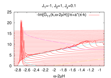
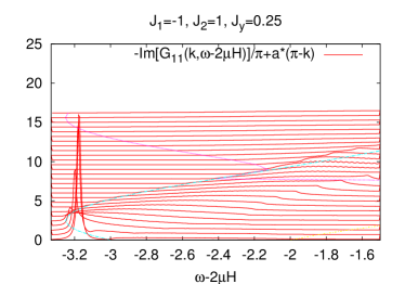
Figure S3: The spectral density of the two-particle Green’s function for a 2D arrangement of unshifted $J_{1}$-$J_{2}$ chains and perpendicular IC interaction, left: $J_{y}\equiv J_{\perp}<J_{cr}$, right: $J_{y}>J_{cr}$.

We see that for small IC couplings the spectral density behaves qualitatively similar to the 1D case, i.e. the peak corresponding to the bound pair lies below the continuum (left panel of Fig. S3), and its dispersion exhibits a minimum at the total momentum $\mathbf{ka}=\pi$ of a pair. We have checked numerically that the minimum position remains at the point $\mathbf{k}_{\pi}=\left(\pi/a,0,0\right)$ for all values of IC satisfying the condition $J_{\perp}<J_{cr}$. On the right panel of Fig. S3 we see that the behavior of the spectral density changes for large enough IC. The bound state is still present near the edge of the Brillouin zone, but its energy is higher than the minimum of the two-particle continuum. It is clear that the critical IC value $J_{cr}$ is defined by the condition

$$\omega_{b}\equiv\omega(\mathbf{k}_{\pi})=\omega_{min},$$ (S27)

where $\omega_{min}=2\left(\mu\mathcal{H}-|J_{1}|h_{s,1}\right)$ is the minimum of the energy of the two-particle continuum, and

$$\begin{array}[]{rcl}h_{s,1}&\equiv&-\Delta_{1}+\alpha\left(\Delta_{2}+1\right)+\\ &+&0.125/\alpha+0.5N_{\mbox{\tiny ic}}\left(j_{\mbox{\tiny ic}}\Delta_{ic}+|j_{\mbox{\tiny ic}}|\right)\ ,\end{array}$$ (S28)

is the critical field of the 1-magnon instability (Eq. (1) of the main text). In order to find the expression for the saturation field $\mathcal{H}_{s}$ as a function of IC $\left|J_{\perp}\right|<J_{cr}$, we need the expression for $\omega_{b}$, which is the position of an isolated pole of the GF

$$\left[G_{\mathbf{a,a}}(\mathbf{k}_{\pi},\omega_{b})\right]^{-1}=0.$$ (S29)

In terms of the effective model $\hat{H}_{tb}(\mathbf{k}_{\pi})$ (S13), $\omega_{b}$ is the energy of the localized impurity level. From Eq. (S17) we see that the nearest-neighbor hopping along the chain vanishes $t_{\mathbf{a}}=J_{1}\cos\frac{\pi}{2}=0$, and the sites with $\mathbf{r}=n\mathbf{a}+m\mathbf{b}+l\mathbf{c}$ having odd and even $n$’s are decoupled. In the subsystem with odd $n$’s, only two impurities of the same strength $\varepsilon_{\mathbf{a}}=J_{1}$ are present at the sites $\pm\mathbf{a}=(\pm a,0,0)$. The effective particle motion is not affected neither by the impurity at the origin (of infinite strength) nor by the impurities at the sites $\mathbf{f}=(0,\pm b,0),(0,0,\pm c)$ with the energies $J_{2}\Delta_{2}$, and $J_{\perp}\Delta_{\perp}$, respectively. Note that this peculiarity has an important consequence: the critical value of the IC given below by Eqs.(S54)-(S57) depends only on the nearest-neighbor exchange anisotropy value $\Delta_{1}$. So, we may immediately write down the expression for the GF (cf. Eq. (49) of Ref. Kuzian and Drechsler, 2007)

$$G_{\mathbf{a,a}}(\mathbf{k}_{\pi},\omega)=\left\{\left[G_{\mathbf{a,a}}^{(0)}(\mathbf{k}_{\pi},\omega)\right]^{-1}-J_{1}\Delta_{1}\right\}^{-1},$$ (S30)

where

$$G_{\mathbf{a,a}}^{(0)}(\mathbf{k}_{\pi},\omega) = \left\langle\phi_{\mathbf{a}}\right|\left(\omega-\hat{T}(\mathbf{k_{\pi}})-\left|\mathbf{0}\right\rangle\varepsilon_{\mathbf{0}}\left\langle\mathbf{0}\right|\right)^{-1}\left|\phi_{\mathbf{a}}\right\rangle$$ (S31)

$$= g_{\mathbf{0}}(\mathbf{k_{\pi}})+g_{2\mathbf{a}}(\mathbf{k_{\pi}})-\frac{2g_{\mathbf{a}}^{2}(\mathbf{k_{\pi}})}{g_{\mathbf{0}}}$$

$$= g_{\mathbf{0}}(\mathbf{k_{\pi}})+g_{2\mathbf{a}}(\mathbf{k_{\pi}}).$$ (S32)

In Eq. (S31) we have used the relation (S25) and Eq. (S32) follows from $g_{\mathbf{a}}(\mathbf{k_{\pi}})=0$, since the vector $\mathbf{a}$ joins two decoupled subsystems. Then Eq. (S29) may be rewritten as

$$G_{\mathbf{a,a}}^{(0)}(\mathbf{k}_{\pi},\omega)=\left(J_{1}\Delta_{1}\right)^{-1}$$ (S33)

Now, using the definition (S22), we may write

$$G_{\mathbf{a,a}}^{(0)}(\mathbf{k}_{\pi},\omega) = \frac{1}{N_{\perp}}\sum_{q_{y},q_{z}}G_{1,1}^{(0)}\left(\pi,\omega-E_{\perp}(\pi,\mathbf{q})\right),$$ (S34)

$$G_{1,1}^{(0)}\left(\pi,\omega\right) = \frac{1}{N_{x}}\sum_{q_{x}}\frac{1+\cos 2q_{x}a}{\omega-E_{1D}(\pi,q_{x})},$$ (S35)

$$E_{1D}(\pi,q_{x}) = 2\left[\mu\mathcal{H}+J_{1}\left(\cos q_{x}a-\Delta_{1}\right)\right.$$ (S36)

$$+\left.J_{2}\left(\cos 2q_{x}a-\Delta_{2}\right)\right],$$

$$E_{\perp}(\pi,\mathbf{q}) = N_{ic}J_{\perp}\left(\gamma_{\mathbf{q}}-\Delta_{\perp}\right),$$ (S37)

where $\gamma_{q}=\cos q_{y}b$ ($\left(\cos q_{y}b+\cos q_{z}c\right)/2$), $N_{\rm ic}=2$(4) for a 2D (3D) geometry, respectively. In the 2D case the summation over $q_{z}$ should be dropped. The 1D GF as given by Eq.  (S35) is easily calculated

$$G_{1,1}^{(0)}\left(\pi,\omega\right) = G(z)/J_{2},$$ (S38)

$$G(z) = \left[z+1-\tau(z)\right]^{-1},$$ (S39)

where we have introduced the dimensionless variable

$$z(\omega)\equiv\left[\omega-2\left(\mu\mathcal{H}-J_{1}\Delta_{1}-J_{2}\Delta_{2}\right)\right]/J_{2},$$ (S40)

and the dimensionless Green’s function of a semi-infinite tight-binding chain $\tau(z)=\left[z-\tau(z)\right]^{-1}$. Now, we search for the solution of Eq. (S30) in the form

$$\omega_{b}=J_{2}\left(z_{b1}+\zeta\right)+2\left(\mu\mathcal{H}-J_{1}\Delta_{1}-J_{2}\Delta_{2}-\frac{1}{2}N_{\rm ic}J_{\perp}\Delta_{\perp}\right),$$ (S41)

where $\zeta$ is unknown, and

$$z_{b1}\equiv-\left(\frac{\Delta_{1}+\alpha}{\alpha}+\frac{\alpha}{\Delta_{1}+\alpha}\right)\quad,$$ (S42)

is the solution for the 1D-problem Kuzian and Drechsler (2007). Note that here we use another definition for the frustration parameter $\alpha\equiv J_{2}/|J_{1}|$ as compared to Ref. Kuzian and Drechsler, 2007.

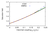
Figure S4: (Color online) The saturation field $h_{s,2}(\alpha,j_{y})=\mu\mathcal{H}_{s}/|J_{1}|$ for a 2D array of chains ($J_{y}\equiv J_{\perp}$) for $\alpha=1$,$\Delta_{1}=1$. Black solid line: the result of analytic Eq.(S52), green short-dashed line: the result of the expansion (S52) up to second order (i.e. $\zeta_{4}$ is neglected), black dashed line: the field of the 1-magnon instability $h_{s,1}$ (S28). Points: DMRG-data and data from the numerical solution of Eq. (S29).

Assuming $\zeta\ll 1$, we rewrite Eq. (S33) in the form

$$\frac{1}{N_{\perp}}\sum_{q_{y},q_{z}}\sum_{m=0}^{\infty}\frac{G^{(m)}}{m!}\left(\zeta-e_{\mathbf{q}}\right)^{m}=-\frac{\alpha}{\Delta_{1}},$$

where $e_{\mathbf{q}}\equiv N_{ic}J_{\perp}\gamma_{\mathbf{q}}/J2$,

$$G^{(m)}\equiv\left(\frac{\partial}{\partial z}\right)^{m}G(z)\mid_{z=z_{b1}}.$$

Note that $G(z_{b1})=-\alpha/\Delta_{1}^{z}$, and keeping only terms with $m\leq 4$, we obtain the equation

$$\zeta G^{\prime}+\frac{1}{2}\left(\zeta^{2}+\overline{e_{\mathbf{q}}^{2}}\right)G^{\prime\prime}$$

$$+\frac{1}{6}\left(\zeta^{3}+3\zeta\overline{e_{\mathbf{q}}^{2}}\right)G^{\prime\prime\prime}$$

$$+\frac{1}{24}\left(\zeta^{4}+6\zeta^{2}\overline{e_{\mathbf{q}}^{2}}+\overline{e_{\mathbf{q}}^{4}}\right)G^{IV} = 0,$$ (S43)

where

$$\overline{e_{\mathbf{q}}^{m}}\equiv\frac{1}{N_{\perp}}\sum_{q_{y},q_{z}}e_{\mathbf{q}}^{m},$$

and we have taken into account that $\overline{e_{\mathbf{q}}}=\overline{e_{\mathbf{q}}^{3}}=0$. The direct calculation yields $\overline{e_{\mathbf{q}}^{2}}=N_{ic}\left(J_{\perp}/J_{2}\right)^{2}$, and $\overline{e_{\mathbf{q}}^{4}}=6\left(J_{\perp}/J_{2}\right)^{4}$ ($36\left(J_{\perp}/J_{2}\right)^{4}$) for 2D(3D) respectively;

$$G^{\prime} = G^{2}\left[\tau^{\prime}-1\right],$$ (S44)

$$G^{\prime\prime} = 2G^{3}\left[\tau^{\prime}-1\right]^{2}+G^{2}\tau^{\prime\prime},$$ (S45)

$$G^{\prime\prime\prime} = 6G^{4}\left[\tau^{\prime}-1\right]^{3}$$ (S46)

$$+ 6G^{3}\left[\tau^{\prime}-1\right]\tau^{\prime\prime}+G^{2}\tau^{\prime\prime\prime},$$

$$G^{IV} = 24G^{5}\left[\tau^{\prime}-1\right]^{4}+36G^{4}\left[\tau^{\prime}-1\right]^{2}\tau^{\prime\prime}$$ (S47)

$$+ 6G^{3}\left(\tau^{\prime\prime}\right)^{2}+8G^{3}\left[\tau^{\prime}-1\right]\tau^{\prime\prime\prime}+G^{2}\tau^{IV},$$

$$\tau^{\prime} = -\frac{\alpha^{2}}{\Delta_{1}\left(\Delta_{1}+2\alpha\right)},$$

$$\tau^{\prime\prime} = -2\left[\frac{\alpha\left(\Delta_{1}+\alpha\right)}{\Delta_{1}\left(\Delta_{1}+2\alpha\right)}\right]^{3},$$

$$\tau^{\prime\prime\prime} = -6\left[\frac{\alpha\left(\Delta_{1}+\alpha\right)}{\Delta_{1}\left(\Delta_{1}+2\alpha\right)}\right]^{4}\frac{\Delta_{1}^{2}+2\Delta_{1}\alpha+2\alpha^{2}}{\Delta_{1}\left(\Delta_{1}+2\alpha\right)},$$

$$\tau^{IV} = -24\frac{\alpha^{5}\left(\Delta_{1}+\alpha\right)^{5}F}{\left[\Delta_{1}\left(\Delta_{1}+2\alpha\right)\right]^{7}},$$

$$F \equiv \Delta_{1}^{4}+4\Delta_{1}^{3}\alpha+9\Delta_{1}^{2}\alpha^{2}+10\Delta_{1}\alpha^{3}+5\alpha^{4}.$$

Substituting the expansion

$$\zeta=\zeta_{1}j_{ic}+\zeta_{2}j_{ic}^{2}+\zeta_{3}j_{ic}^{3}+\zeta_{4}j_{ic}^{4},$$ (S48)

($j_{ic}\equiv J_{\perp}/|J_{1}|$) into (S43), we obtain $\zeta_{1}=\zeta_{3}=0$, and

$$\zeta_{2} = -\frac{N_{ic}G^{\prime\prime}}{2\alpha^{2}G^{\prime}}\ ,$$ (S49)

$$= -\frac{N_{ic}\left(\Delta_{1}+\alpha\right)}{\alpha\left[\Delta_{1}\left(\Delta_{1}+2\alpha\right)\right]^{2}}\left[\Delta_{1}^{2}+3\Delta_{1}\alpha+3\alpha^{2}\right],$$ (S50)

$$\zeta_{4} = -\frac{1}{G^{\prime}}\left[\frac{G^{\prime\prime}}{2}\zeta_{2}^{2}-\frac{N_{ic}G^{\prime\prime\prime}}{2\alpha^{2}}\zeta_{2}+\frac{G^{IV}}{24\beta^{4}}\overline{e_{\mathbf{q}}^{4}}\right].$$ (S51)

At the saturation field, the $\omega_{b}$ in the right-hand side of Eq. (S41) vanishes, and we obtain

$$h_{s,2} = h_{s,2}^{\rm 1D}+\frac{N_{\rm ic}}{2}j_{\rm ic}\Delta_{\perp}-\frac{\alpha}{2}\left(\zeta_{2}j_{\rm ic}^{2}+\zeta_{4}j_{\rm ic}^{4}\right)\ ,\$$ (S52)

$$h_{s,2}^{\rm 1D} = -\Delta_{1}+\alpha\Delta_{2}-\frac{\alpha}{2}z_{\rm b1}\quad,$$

where $h_{s}\equiv\mu\mathcal{H}_{s}/|J_{1}|$. Eq. (S52) coincides with Eq. (3) of the main text with $\eta_{i}=-\alpha\zeta_{i}/2$. Its validity is demonstrated in Fig. S4. As an example, we have chosen the 2D case and $\alpha=1$, i.e. the optimal region for the existence of the nematic phase, where $j_{\rm cr}\approx 0.167$.

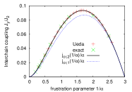
Figure S5: Boundary between the 1- and 2- magnon phases for the 3D case ($J_{y}\equiv J_{\perp}$). Points: the numerical results from this work and from Ref. Ueda and Totsuka, 2009

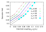
Figure S6: The saturation field $h_{s,2}$ for the 3D case for $\alpha=0.5$ ($J_{y}\equiv J_{\perp}$). The easy-axis anisotropy of the NN coupling is taken into account. The meaning of the lines is the same as in Fig. S4. Points: DMRG-data ($\Delta_{1}\neq 1$), and the data from a numerical solution of Eq. (S29) ($\Delta_{1}=1$)

.

For small $j_{\perp}=J_{\perp}/|J_{1}|$ the second order expansion reproduces well the DMRG data which coincide with the results from a numerical solution of Eq. (S29). Naturally, for larger interchain coupling $j_{\perp}>0.15$ the fourth order expansion is needed.

The boundary between the 1-magnon and the 2-magnon phases is obtained by solving the equation $h_{s,2}(j_{\rm cr})=h_{s,1}(j_{\rm cr,})$ for the critical IC $j_{\rm cr}$. If one retains only the linear term in the expansion in powers of the IC given by (S52), we obtain (cf. Eq. (51) in Ref. Syromyatnikov, 2012)

$$|j_{\rm cr,1}|=\frac{4\alpha\Delta_{1}^{2}-\Delta_{1}-\alpha}{4N_{\rm ic}\alpha\left(\Delta_{1}+\alpha\right)}.$$ (S53)

This approximation demonstrates the qualitative behaviour of $j_{\rm cr}$ as a function of the anisotropy and the frustration parameters $\Delta_{1}$ and $\alpha$, respectively. Practically, a fully quantitative agreement with our numerical data is achieved, if we account also for the quadratic term in Eq. (S52)

$$|j_{cr,2}|=\frac{1}{2\alpha\zeta_{2}}\left(-N_{ic}+\sqrt{N_{ic}^{2}+4N_{ic}\alpha\zeta_{2}|j_{cr,1}|}\right).$$ (S54)

It is convenient to normalize the couplings on $J_{2}>0$, and introduce $\kappa\equiv 1/\alpha$, which measures the attraction provided by the FM $J_{1}$. Using the same normalization for the IC, too, we write $y\equiv J_{\perp}/J_{2}=j_{ic}/\alpha$. Then the Eqs.  (S50), (S53), and (S54) may be rewritten as

$$\zeta_{2} = -\frac{N_{ic}\left(\kappa\Delta_{1}+1\right)}{\left[\Delta_{1}\left(\kappa\Delta_{1}+2\right)\right]^{2}}\left[\kappa 2\Delta_{1}^{2}+3\Delta_{1}\kappa+3\right],$$ (S55)

$$|y_{cr,1}| = \frac{\kappa^{2}\left(4\Delta_{1}^{2}-\kappa\Delta_{1}-1\right)}{4N_{ic}\left(\kappa\Delta_{1}+1\right)},$$ (S56)

$$|y_{cr,2}| = \frac{\kappa^{2}}{2\zeta_{2}}\left(-N_{ic}+\sqrt{N_{ic}^{2}+\frac{4N_{ic}\zeta_{2}|y_{cr,1}|}{\kappa^{2}}}\right).$$ (S57)

A comparison of the results of the approximate analytic Eqs. (S56) and (S57) with the numerical data is shown in Fig. S5. Note the high accuracy achieved already in the second order of the IC in Eq. (S52). Finally, an example of the saturation field dependence on the anisotropy parameter is shown in Fig. S6.

References

Castelnovo et al. (2008)
C. Castelnovo,
R. Moessner,
and S. L.
Sondhi, Nature
451, 42 (2008).
Lacroix et al. (2011)
C. Lacroix,
P. Mendels, and
F. Mila, eds.,
Introduction to Frustrated Magnetism
(Springer-Verlag, Berlin, Heidelberg,
2011).
Chubukov (1991)
A. Chubukov,
Phys. Rev. B 44,
4693 (1991).
Kecke et al. (2007)
L. Kecke,
T. Momoi, and
A. Furusaki,
Phys. Rev. B 76,
060407 (2007).
Vekua et al. (2007)
T. Vekua,
A. Honecker,
H.-J. Mikeska,
and
F. Heidrich-Meisner,
Phys. Rev. B 76,
174420 (2007).
Hikihara et al. (2008)
T. Hikihara,
L. Kecke,
T. Momoi, and
A. Furusaki,
Phys. Rev. B 78,
144404 (2008).
Sudan et al. (2009)
J. Sudan,
A. Lüscher,
and
A. Läuchli,
Phys. Rev. B 80,
140402 (2009).
Dmitriev and Krivnov (2009)
D. Dmitriev and
V. Krivnov,
Phys. Rev. B 79,
054421 (2009).
Zhitomirsky and Tsunetsugu (2010)
M. Zhitomirsky and
H. Tsunetsugu,
EPL (Europhys. Lett.) 92,
37001 (2010).
Svistov et al. (2011)
L. Svistov,
T. Fujita,
H. Yamaguchi,
S. Kimura,
K. Omura,
A. Prokofiev,
A. I. Smirnov,
Z. Honda, and
M. Hagiwara,
"Pis’ma Zh. Eksp. Teor. Fiz."
93, 21 (2011).
Syromyatnikov (2012)
A. Syromyatnikov,
Phys. Rev. B 86,
014423 (2012).
Sizanov and Syromyatnikov (2013)
A. Sizanov and
A. Syromyatnikov,
Phys. Rev. B 87,
014410 (2013).
Enderle et al. (2005)
M. Enderle,
C. Mukherjee,
B. Fåk,
R. K. Kremer,
J.-M. Broto,
H. Rosner,
S.-L. Drechsler,
J. Richter,
J. Malek,
A. Prokofiev,
et al., EPL (Europhys. Lett.)
70, 237 (2005).
Büttgen et al. (2007)
N. Büttgen,
H.-A. Krug von Nidda,
L. Svistov,
L. Prozorova,
A. Prokofiev,
and
W. Aßmus,
Phys. Rev. B 76,
014440 (2007).
Büttgen et al. (2010)
N. Büttgen,
W. Kraetschmer,
L. E. Svistov,
L. A. Prozorova,
and
A. Prokofiev,
Phys. Rev. B 81,
052403 (2010).
Hagiwara et al. (2011)
M. Hagiwara,
L. Svistov,
T. Fujita,
H. Yamaguchi,
S. Kimura,
K. Omura,
A. Prokofiev,
A. I. Smirnov,
and Z. Honda,
J. of Phys.: Conf. Ser. 320,
012049 (2011).
Drechsler et al. (2007)
S.-L. Drechsler,
O. Volkova,
A. N. Vasiliev,
N. Tristan,
J. Richter,
M. Schmitt,
H. Rosner,
J. Málek,
R. Klingeler,
A. A. Zvyagin,
et al., Phys. Rev. Lett.
98, 077202
(2007).
Schmitt et al. (2009)
M. Schmitt,
J. Málek,
S.-L. Drechsler,
and H. Rosner,
Phys. Rev. B 80,
205111 (2009).
Matsuda et al. (2001)
M. Matsuda,
H. Yamaguchi,
T. Ito,
C. H. Lee,
K. Oka,
Y. Mizuno,
T. Tohyama,
S. Maekawa, and
K. Kakurai,
Phys. Rev. B 63,
180403 (2001).
Kuzian et al. (2012)
R. Kuzian,
S. Nishimoto,
S.-L. Drechsler,
J. Málek,
S. Johnston,
J. van den Brink,
M. Schmitt,
H. Rosner,
M. Matsuda,
K. Oka, et al.,
Phys. Rev. Lett. 109,
117207 (2012).
Wolter et al. (2012)
A. Wolter,
F. Lipps,
M. Schäpers,
S.-L. Drechsler,
S. Nishimoto,
R. Vogel,
V. Kataev,
B. Büchner,
H. Rosner,
M. Schmitt,
et al., Phys. Rev. B
85, 014407
(2012).
Willenberg et al. (2012)
B. Willenberg,
M. Schäpers,
K. C. Rule,
S. Süllow,
M. Reehuis,
H. Ryll,
B. Klemke,
K. Kiefer,
W. Schottenhamel,
B. Büchner,
et al., Phys. Rev. Lett.
108, 117202
(2012).
Hase et al. (2004)
M. Hase,
H. Kuroe,
K. Ozawa,
O. Suzuki,
H. Kitazawa,
G. Kido, and
T. Sekine,
Phys. Rev. B 70,
104426 (2004).
Lorenz et al. (2009)
W. Lorenz,
R. Kuzian,
S.-L. Drechsler,
W.-D. Stein,
N. Wizent,
G. Behr,
J. Málek,
U. Nitzsche,
H. Rosner,
A. Hiess,
et al., EPL (Europhys. Lett.)
88, 37002 (2009).
Nishimoto et al. (2011)
S. Nishimoto,
S.-L. Drechsler,
R. O. Kuzian,
J. van den Brink,
J. Richter,
W. E. A. Lorenz,
Y. Skourski,
R. Klingeler,
and
B. Büchner,
Phys. Rev. Lett. 107,
097201 (2011).
Kuzian and Drechsler (2007)
R. Kuzian and
S.-L. Drechsler,
Phys. Rev. B 75,
024401 (2007).
(27)
See supplementary materials at [URL will be inserted by
publisher] for the details of derivation of Eq. (3), and the account of
anisotropies of other exchange couplings.
Nishimoto
et al. (2012a)
S. Nishimoto,
S.-L. Drechsler,
R. Kuzian,
J. Richter,
J. Málek,
M. Schmitt,
J. van den Brink,
and H. Rosner,
EPL (Europhys. Lett. 98,
37007 (2012a).
Nishimoto
et al. (2012b)
S. Nishimoto,
S.-L. Drechsler,
R. Kuzian,
J. Richter, and
J. van den Brink,
J. Phys.: Conf. Ser. 400,
032069 (2012b).
Tornow et al. (1999)
S. Tornow,
O. Entin-Wohlman,
and A. Aharony,
Phys. Rev. B 60,
10206 (1999).
Yushankhai and Hayn (1999)
V. Yushankhai and
R. Hayn, EPL
(Europhys. Lett.) 47, 116
(1999).
Kataev et al. (2001)
V. Kataev,
K.-Y. Choi,
M. Grüninger,
U. Ammerahl,
B. Büchner,
A. Freimuth, and
A. Revcolevschi,
Phys. Rev. Lett. 86,
2882 (2001).
Heidrich-Meisner
et al. (2009)
F. Heidrich-Meisner,
I. McCulloch,
and
A. Kolezhuk,
Phys. Rev. B 80,
144417 (2009).
White (1992)
S. White,
Phys. Rev. Lett. 69,
2863 (1992).
Nishimoto et al. (2010)
S. Nishimoto,
M. Nakamura,
A. O’Brien, and
P. Fulde,
Phys. Rev. Lett. 104,
196401 (2010).
Stoudenmire and White (2012)
E. Stoudenmire and
S. R. White,
Ann. Rev. of Cond. Mat. Phys.
3, 111 (2012).
Zinke et al. (2009)
R. Zinke,
S.-L. Drechsler,
and J. Richter,
Phys. Rev. B 79,
094425 (2009).
(38)
Here and below, we use the presentation in terms of
interpenetrating single Heisenberg chains coupled by , which includes
explicitely both the limit of two decoupled Heisenberg chains =0,
and the quantum critical point =4 .
Ueda and Totsuka (2009)
H. Ueda and
K. Totsuka,
Phys. Rev. B 80,
014417 (2009).
Gippius et al. (2004)
A. Gippius,
E. Morozova,
A. Moskvin,
A. Zalessky,
A. Bush,
M. Baenitz,
H. Rosner, and
S.-L. Drechsler,
Phys. Rev. B 70,
020406 (2004).
Masuda et al. (2005)
T. Masuda,
A. Zheludev,
B. Roessli,
A. Bush,
M. Markina, and
A. Vasiliev,
Phys. Rev. B 72,
014405 (2005).
Drechsler et al. (2006)
S. Drechsler,
J. Richter,
A. Gippius,
A. Vasiliev,
A. Bush,
A. Moskvin,
J. Málek,
Y. Prots,
W. Schnelle, and
H. Rosner,
EPL (Europhys. Lett.) 73,
83 (2006).
Mihály et al. (2006)
L. Mihály,
B. Dóra,
A. Ványolos,
H. Berger, and
L. Forró,
Phys. Rev. Lett. 97,
067206 (2006).
Enderle et al. (2010)
M. Enderle,
B. Fåk,
H.-J. Mikeska,
R. K. Kremer,
A. Prokofiev,
and W. Assmus,
Phys. Rev. Lett. 104,
237207 (2010).
Drechsler et al. (2011)
S.-L. Drechsler,
S. Nishimoto,
R. Kuzian,
J. Málek,
W. Lorenz,
J. Richter,
J. van den Brink,
M. Schmitt, and
H. Rosner,
Phys. Rev. Lett. 106,
219701 (2011).
Yasui et al. (2011)
S. Yasui,
Y. Yanagisawa,
M. Sato, and
I. Terasaki,
J. of Phys.: Conf. Ser. 320,
012087 (2011).
Economou (2006)
E. Economou,
Green’s Functions in Quantum Physics
(Springer-Verlag, Berlin, Heidelberg,
2006).
Supplementary Material for