A new method for the extraction of mid-infrared $\gamma$-ray emitting candidate blazars

Abstract

We present a new method for identifying blazar candidates by examining the locus, i.e. the region occupied by the Fermi $\gamma$-ray blazars in the three-dimensional color space defined by the WISE infrared colors. This method is a refinement of our previous approach that made use of the two-dimensional projection of the distribution of WISE $\gamma$-ray emitting blazars (the Strip) in the three WISE color-color planes (Massaro et al., 2012a). In this paper, we define the three-dimensional locus by means of a Principal Component (PCs) analysis of the colors distribution of a large sample of blazars composed by all the ROMA-BZCAT sources with counterparts in the WISE All-Sky Catalog and associated to $\gamma$-ray source in the second Fermi LAT catalog (2FGL) (the WISE Fermi Blazars sample, WFB). Our new procedure, as reported in (D’Abrusco et al., 2013), yields a total completeness of $c_{\mathrm{tot}}\!\sim$81% and total efficiency of $e_{\mathrm{tot}}\!\sim$97%.

I Introduction

Unveiling the nature of the Unidentified Gamma-ray Sources (UGS) is one of the main scientific objectives of the ongoing Fermi $\gamma$-ray mission. Recently, several attempts have been performed to associate or characterize the UGSs, either using X-ray observations (e.g., Mirabal, 2009; Mirabal & Halpern, 2009) or with statistical approaches (e.g. Mirabal et al., 2010; Ackermann et al., 2012). Nevertheless, according to Nolan et al. (2012), 31% of the $\gamma$-ray sources in the second Fermi LAT catalog (2FGL) remain unidentified and many of these unidentified sources could be blazars, since blazars are known to dominate the $\gamma$-ray sky (e.g. Hartman et al., 1999; Abdo et al., 2010), and among the 1297 associated sources within the 2FGL, 805 (62%) are known blazars Nolan et al. (2012). Therefore it is important to devise an efficient means of identifying candidate blazars among these sources.

Blazars come in two main classes: the BL Lac objects, which have featureless optical spectra, and the more luminous Flat-Spectrum Radio Quasars which, typically, show prominent optical spectral emission lines (Stickel et al., 1991). In the following discussion, we label the BL Lac objects as BZBs and the Flat-Spectrum Radio Quasars as BZQs, following the nomenclature of the Multi-wavelength Catalog of blazars (ROMA-BZCAT, Massaro et al., 2009).

Using the preliminary data release of the Wide-field Infrared Survey Explorer (WISE) (see  Wright et al., 2010, for more details), we showed that the $\gamma$-ray blazar population occupies a distinctive region of the WISE color parameter space (called the WISE Gamma-ray Strip Massaro et al. (2011); D’Abrusco et al. (2012)). Taking advantage of the much larger data set now available thanks to the WISE All-Sky archive, released in March 2012, in this work we present a revisited definition of the region occupied by the $\gamma$-ray blazars. We will refer to the 3-dimensional region occupied by the $\gamma$-ray emitting blazars as the locus while we will continue to indicate the 2-dimensional projection of the locus in the $[3.4]\!-\![4.6]$ vs $[4.6]\!-\![12]$ $\mu$m color-color plane as WISE Gamma-ray Strip. In this proceeding we determine a geometrical description of the WFB locus in the space generated by the Principal Components of their distribution in the WISE color space and apply our association procedure the whole sample of blazars that belong to the 2FGL.

II The WISE Fermi Blazars sample

We found 3032 out of 3149 (i.e., 96.3% of the ROMA-BZCAT) blazars with an IR counterpart within 3.3^′′ in the WISE All-Sky data archive. In this sample, there are only 2 multiple matches out of 3032 spatial associations, for which we used the IR data of the closest WISE source in the following analysis. The probability of a chance associations for these 3032 is $\sim\!$ 3.3%, implying that $\sim\!$ 100 sources associated within the above radius could be spurious associations.

Of these 3032 blazars, 1172 are BZBs, including 919 BL Lacs and 253 BL Lac candidates, 1642 are BZQs and 218 are BZUs. It is also worth noticing that all the blazars associated between the ROMA-BZCAT and the WISE all-sky data release are detected in the first two filters at 3.4 and 4.6 $\mu$m. Among the 3032 selected blazars, only 673 have a counterpart in the $\gamma$-rays according to the 2FGL and to the CLEAN sample presented in the second Fermi LAT Catalog of active galactic nuclei (2LAC; Ackermann et al., 2011). 637/673 (i.e., 94.7%) of these blazars (333 BZBs, 277 BZQs, and 27 BZUs) are detected in all four WISE bands. As in (Massaro et al., 2012b) the sample of $\gamma$-ray emitting blazars in the ROMA-BZCAT catalog was derived excluding the BZUs sources from our sample of $\gamma$-ray loud blazars. For this reason, the final WFB sample includes only 610 WISE sources out of 673 WISE counterparts. We have used the WFB sample to characterize the model of the locus in the WISE color space.

III The locus parametrization

The new parametrization of the WFB locus is based on a new model of the locus in the PCs space generated by the WISE colors of the WFB WISE counterparts, and on revised definition of the statistical quantity used to evaluate the compatibility of a generic WISE source with the locus model, the score. The distribution of the WFB sources in the three-dimensional WISE color space is axisymmetric along a slew line (see Figure 1), so that a simple geometrical description of the locus can be determined in the PCs space.

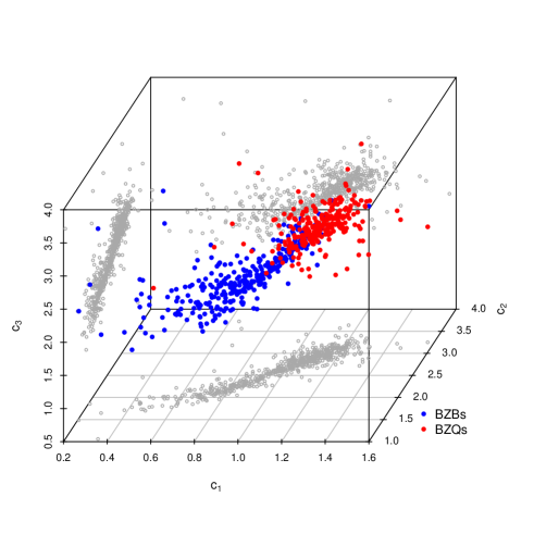
Figure 1: Scatterplot of the WFB sources in the three-dimensional WISE color space. The spectral class of the WFB sources is color-coded, while the gray points represent the projections of the WFB sample in the three color planes generated by WISE colors.

Principal Component Analysis (PCA) uses an orthogonal transformation to convert a set of observations of possibly correlated variables into a set of values of linearly uncorrelated variables, the PCs. This transformation $T\!:\!(c_{1},c_{2},c_{3})\rightarrow(\mathrm{PC}_{1},\mathrm{PC}_{2},\mathrm{PC}_{3})$ is defined so that the first PC (PC₁) accounts for as much of the variance in the data as possible, and each following component (PC₂, PC₃, etc. up to the dimensionality of the initial space) has the highest variance possible under the constraint that it is orthogonal to the preceding components. In our case, the WFB sources in the three-dimensional PCs space based on their color distributions lie almost perfectly along the PC₁ axis and are distributed symmetrically in the PC₂ vs PC₃ plane around the PC₁ line. Based on the shape of the locus in the PCs space, we choose to define its geometrical model using a cylindrical parametrization, with axis aligned along the PC₁ axis (see Fig 3). The locus, as a whole, is modeled by three distinct cylinders: the first two of these cylindrical regions are dominated by BZB and BZQ sources respectively, while the third cylinder is defined as the region where the WFB population is mixed in terms of spectral classes (the Mixed region, hereinafter).

The upper and lower boundaries of the model along the PC₁ axis have been determined requiring that 90% of the total number of WFB sources is contained within the boundaries of the cylinder, with 5% of the sources outside of the boundaries of the model on each side of the model along the PC₁ axis. The boundaries of the Mixed section along the PC₁ axis have been defined by requiring that, in this region, the fraction of either spectral class is smaller than 80% of the total number of WFB sources. The three boundaries along the PC₁ axis defining the three sections of the WFB locus model are shown in Figure. 2.

Figure 2: Boundaries of the three sections of the WFB locus in the PCs space along the PC₁ axis. The solid black line represent the “purity” of the WFB population, i.e. the fraction of the dominant spectral class relative to the other spectral class. The solid red and blue lines represent the fraction of BZQs and BZBs sources, while the histogram in the background represents the normalized density of the distribution of the whole WFB sample along the PC₁ axis. The horizontal green line shows the threshold used to determine the boundaries of the mixed region.

The variances of the distribution of the WFB distribution in the PC space along the second and third PCs are $\sigma^{2}_{\mathrm{PC_{2}}}\!=\!0.61$ and $\sigma^{2}_{\mathrm{PC_{3}}}\!=\!0.58$ respectively. Based on this fact, we have modeled the bases of the cylinders as circles centered on the axis of the first principal component PC₁ (the variance of the WFB distribution along PC₁ is $\sigma^{1}_{\mathrm{PC_{3}}}\!=\!1.53$). The radii of the circular bases of each of the three cylinders representing the three different sections of the WFB locus in the PCs space have been determined independently as the radii containing the 90% of the WFB sources in each section. The radii of each of the three cylinders are defined in the plane generated by the PC₂ and PC₃ axes and evaluate d as $R=\sqrt{\mathrm{PC}_{2}^{2}\!+\!\mathrm{PC}_{3}^{2}}$.

III.1 The score

The distance of a generic WISE source to the model of the WFB locus in the PCs space can be evaluated quantitatively using a numeric quantity that we call the score. The generic WISE source with colors $(\tilde{c}_{1},\tilde{c}_{2},\tilde{c}_{3})$ can be projected onto the PCs space by applying the orthogonal transformation determined by the PCA performed on the WFB sample for the modelization of the WFB locus in the PCs space. Thus, the position of the generic WISE source in the PCs space is determined by the PCs values $(\tilde{\mathrm{PC}}_{1},\!\tilde{\mathrm{PC}}_{2},\!\tilde{\mathrm{PC}}_{3})\!=\!T(\tilde{c}_{1},\!\tilde{c}_{2},\!\tilde{c}_{3})$. To take into account the uncertainties on the values of the WISE colors, the standard deviations on each color are also projected onto the PCs space and are used to define the error bars on the position of the source in the PCs space: $(\pm\sigma_{\tilde{\mathrm{PC}}_{1}},\!\pm\sigma_{\tilde{\mathrm{PC}}_{2}},\!\pm\sigma_{\tilde{\mathrm{PC}}_{3}})\!=\!T(\pm\sigma_{\tilde{c}_{1}},\!\pm\sigma_{\tilde{c}_{2}},\!\pm\sigma_{\tilde{c}_{3}})$. We simply assume that the generic WISE source is represented in the PCs space by the ellipsoid generated by the segments with extremes $\mathrm{PC}_{i}\pm\sigma_{\mathrm{PC}_{i}}$, hereinafter the uncertainty ellipsoid. Each of the six points at the extremes of the axes of the uncertainty ellipsoid in the PCs space will be generically called extremal point. The possible positions of the uncertainty ellipsoid associated with a generic WISE source relative to each of the three cylinders of the locus model (schematically shown in Figure 3 for one two-dimensional section of the PCs space) fall in one of the following cases: six extremal points within a cylinder (point A in Figure 3); five extremal points within a cylinder (point B in Figure 3); three extremal points within a cylinder (point C in Figure 3); one extremal point within a cylinder (points D in Figure 3); no extremal points within any cylinder (points F in Figure 3). Other combinations are not possible because the axes of the uncertainty ellipsoids are either parallel or orthogonal to the PC₁ axis of the PCs space. Points with any number of extremal points within two cylinders (like point E in Figure 3) are assigned a distinct score value for either cylinder according to the number of extremal points contained in each one.

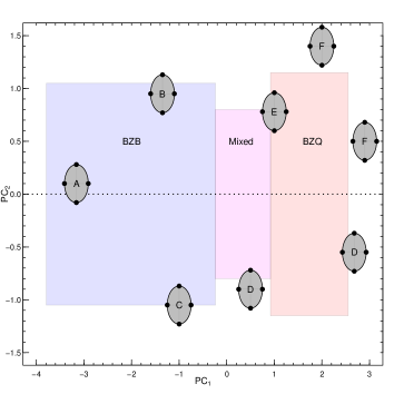
Figure 3: Schematic representation of the possible positions of the uncertainty ellipsoid of a generic WISE source in the PCs space relative to the cylindrical models of the WFB locus (see descriptions of the different cases in the text).

The score $s$ for a generic WISE source with $n$ extremal points contained in one of the three sections of the WFB locus model is defined as:

$$\mathrm{s}=\frac{1}{6^{\phi}}\cdot\!n^{\phi}$$

where $\phi$ is the index of the score assignment law. This is a simple generalization of the most natural choice that would assign to each extremal point within the locus model 1/6, defining the total score of a source as linearly proportional to the number of extremal points within the model cylinders. This behavior is obtained in the general equation when $\phi\!=\!1$. Changing the value of $\phi$ is useful to tweak the performances of the association procedure in terms of the purity and completeness of the final sample of candidate blazars.

So far, the score assigned to a generic WISE source can take one of six different values determined by the score assignment law in Equation III.1. To penalize the WISE sources with large uncertainties on the observed colors (and, in turn, large volume of the uncertainty ellipsoid in the PCs space) relatively to other WISE sources with the same number of extremal points contained in the locus model but smaller errors, we multiply the score obtained using Eq. III.1 by the ratio of the absolute values of the logarithms of the volume of the uncertainty ellipsoid of the source considered and of the volume of the largest uncertainty ellipsoid for WFB sources. Thus, for each of the three regions of the locus model, the weighted score is defined as:

$$\mathrm{s}_{w}=\mathrm{s}\!\cdot\frac{\|\log{V}\|}{\|\log{(\mathrm{max(V_{\mathrm{WFB}})})}\|}$$

where $V_{\mathrm{WFB}}$ are the volumes of the uncertainty ellipsoids of the WFB sources in the PCs space calculated as $V_{\mathrm{WFB}}\!=\!\frac{4}{3}\pi\sigma_{\mathrm{PC}_{1}}\sigma_{\mathrm{PC}_{1}}\sigma_{\mathrm{PC}_{3}}$, and $V$ is the volume of the uncertainty ellipsoid in the PCs space of the generic WISE source considered. The logarithms of the volumes of the uncertainty ellipsoids are used to take into account the large number of order of magnitude potentially spanned by the differences between the volumes (always smaller than one in the PCs space though). The above definition of the weighted score also has the effect of mapping the discrete distribution of scores calculated according to assignment law Equation III.1 into a continuous distribution that allows a finer classification of the candidate blazars.

IV Selection of the candidate blazars

The procedure for the evaluation of the scores based on the new parametrization of the WFB locus discussed in the previous section is used to associate high-energy sources to WISE candidate blazars. The WISE colors and their uncertainties for all the sources found in the WISE All-Sky photometry catalog within the region of positional uncertainty (hereinafter the Search Region - SR) of a given high-energy source and detected in all four WISE filters are retrieved, and the scores of these WISE sources are calculated as described in Section III.1. Then, these sources are split among different classes according to the values of the their scores $s_{b}$, $s_{m}$ and $s_{q}$ for the BZB, Mixed and BZQ regions of the WFB locus model in the PCs space respectively. For each locus region, every source is assigned to class A, class B, class C or is marked as an outlier based on its score values and relative to the threshold scores values defined as the 30%, 60% and 90% percentiles of the distributions of scores in the three regions of the locus for the WFB sources (see Figure 4). The classes are sorted according to decreasing probability of the WISE source to be compatible with the model of the WFB locus: class A sources are considered the most probable candidate blazars for the high-energy source in the SR, while class B and class C sources are less compatible with the WFB locus but are still deemed as candidate blazars. In more details, class A candidate blazars have score $s\leq s_{90\%}$, class B candidate blazars have score $s_{60\%}\!\leq\!s\leq\!s_{90\%}$ and class C candidate blazars have score $s_{30\%}\leq s\leq s_{60\%}$ for each region. The other sources considered outliers are discarded. The values of the score thresholds derived from the score distributions of WFB sources for the three regions of the locus model are reported in Table LABEL:tab:thresholds and shown in Figure 4 overplotted to the histograms of the score distributions of the WFB sources assigned to each of the three locus regions.

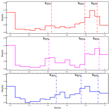
Figure 4: Histograms of distributions of score values calculated for the sources in the WFB sample for the three regions of the locus dominated respectively by the BZQs, the BZBs and in the mixed region (upper, mid and and lower panels respectively). The three vertical lines in each panel represent $s_{30\%}$, $s_{60\%}$ and $s_{90\%}$. These thresholds have been used to define the classes of candidate blazars (see text).

Table 1: Values of the score thresholds $s_{30\%}$, $s_{60\%}$ and $s_{90\%}$, used for the association experiments described in this proceedings. These values are determined as the 30%-th, 60%-th and 90%-th percentiles of the scores of the WFB sample divided by BZB, Mixed and BZB mixed regions.

	BZB	Mixed	BZQ
$s_{30\%}$	0.48	0.44	0.41
$s_{60\%}$	0.75	0.79	0.79
$s_{90\%}$	0.93	0.92	0.94

The choice of the percentiles used to define the classes of candidate blazars is arbitrary and can be changed to allow for more conservative (higher purity of the sample of candidates) or more complete (lower purity of the sample of candidates) selections of candidate blazars in the SRs associated with unidentified high-energy sources.

IV.1 Associations

In our association procedure, the presence of WISE background sources with score values that would qualify them as candidate blazars but that are not located within the SR of the unidentified high-energy source is taken into account by assessing the number and type of spurious associations from sources within a local background region for each unassociated source. For a generic SR of radius $r_{\mathrm{SR}}$, we define the background region (BR) as an annulus of outer radius $r_{\mathrm{BR}}\!=\!\sqrt{2}\!\cdot\!r_{\mathrm{SR}}$ and inner radius equal to the SR radius and centered on the center of the SR. The SR and BR have same area by definition. Within a given SR, all WISE sources detected in all four WISE filters are assigned a score value for each region of the locus model, and successively ranked in classes using the same thresholds used to classify the sources within the SR. An example of a generic SR and associated background region is shown in Figure 5, where the candidate blazar and the spurious BR candidate blazar are colored according to their class membership as defined in Section IV.

For every unassociated high-energy source, our method produces all candidate blazars (sources classified as class A, class B or class C candidate) in the SR. All candidate blazars located in the BR of the high-energy sources are also provided and can be used to evaluate the chance of spurious associations as a function of the class of the candidate blazars.

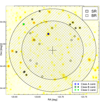
Figure 5: Results of the association procedure for a generic unassociated high-energy source superimposed on the image of the WISE sky around the position of the unassociated $\gamma$-ray source as seen in the $[3.4]\mu$m band. The inner circle represents the Search Region (SR) of the high-energy source while the outer circle delimits the annulus used as Background Region (BR). The open circles in the SR represent the sources of the WISE All-Sky catalog detected in all four WISE filters for which the scores have been evaluated (the sources not marked by symbols in the image are not detected in at least one of the four WISE filters and have not been considered for the score evaluation). The solid circle represents the candidate blazar found within the SR and its color indicates that it is class A candidate blazar.

V Conclusions

In this proceeding we have described the WFB sample of $\gamma$-ray emitting WISE blazars, gathered using the new WISE All-Sky release, the 2FGL catalog and the latest release of the ROMA-BZCAT catalog. Then, we have presented a new association procedure for the unidentified high-energy sources based on a new model of the locus occupied by WFB sample in the three-dimensional PCs space generated by the distribution of WFB WISE sources in the WISE color space. We defined a quantitative measure of the compatibility of a generic WISE source with the locus model and expounded the new association procedure. This method can select candidate blazars classified as BZB or BZQ candidates and ranked according to the likelihood of each candidate of being an actual blazar. We also investigated the possibility of spurious associations by determining the number and class of WISE sources compatible with the model of the WFB locus in background regions defined around the SR of each high-energy source.

The performances of the method in terms of the efficiency and completeness have been estimated in D’Abrusco et al. (2013), yielding a total efficiency $e_{\mathrm{tot}}\!\simeq\!97\%$ and total completeness $c_{\mathrm{tot}}\!\simeq\!81\%$ respectively. By using a $K$-fold cross-validation approach, we have also estimated the efficiency and completeness as functions of the WISE colors and galactic coordinates of the candidate blazars.

In (D’Abrusco et al., 2013), we have presented the catalog of candidate blazars associated with the new procedure to the 2FGL $\gamma$-ray sources included in the WFB sample, used to define the new model of the locus. We have also discussed the catalog of candidate blazars obtained by applying the new association procedure to the 2FB sample, composed of all clean $\gamma$-ray sources associated with blazars in the 2FGL catalog but not contained in the WFB sample. We will make the code for the association and both catalogs of candidate blazars publicly available.