Electronic spectral properties of the two-dimensional infinite-$U$ Hubbard model

Abstract

A strong-coupling series expansion for the Green’s function and the extremely correlated Fermi liquid (ECFL) theory are used to calculate the moments of the electronic spectral functions of the infinite-$U$ Hubbard model. Results from these two complementary methods agree very well at both low densities, where the ECFL solution is the most accurate, and at high to intermediate temperatures, where the series converge. We find that a modified first moment, which underestimates the contributions from the occupied states and is accessible in the series through the time-dependent Green’s function, best describes the peak location of the spectral function in the strongly correlated regime. This is examined by the ECFL results at low temperatures, where it is shown that the spectral function is largely skewed towards the occupied states.

I Introduction

A long-standing theme in the dynamics of strongly interacting systems is the reconstruction of dynamics from the knowledge of the first few moments. h_mori_65 Its appeal lies in the relative ease with which these moments can be computed, in contrast to computing the complete dynamical correlation functions. The method of moments works well in cases where the qualitative features of the correlation functions are somewhat understood by other arguments, including conservation laws in the case of spin dynamics. In the important problem of the strong-coupling Hubbard model, the moments are dominated by the energy scale $U$, w_nolting_72 the on-site repulsive Coulomb interaction, and hence rendered useless. In contrast, for the $t$-$J$ model embodying extreme correlations, i.e., $U\to\infty$ at the very outset, a better prospect exists. The moments are blind to the scale of $U$, since it does not occur in the Hamiltonian, and therefore one expects them to be meaningful in determining the broad features of the dynamics. With this in mind, we study a simple version of the $t$-$J$ model by focusing on $J=0$, which is identical to the $U=\infty$ Hubbard model, thereby making more tools available for the analysis. As we show in what follows, we have developed the capability to compute the moments of the electron spectral function of this model by utilizing series expansions. domb ; series Experiments using angle-resolved photoemission spectroscopy (ARPES) gweon ; johnson ; zx ; jc directly measure this spectral function, providing an added impetus.

An independent source of information about the electronic spectral function is the recent analytical theory of extremely correlated Fermi liquids (ECFL). This theory has been developed in recent publications, ecfl ; hansen-shastry and several results of the model pertaining to the detailed line shapes find close agreement with experiment. gweon On the calculational front, the theory provides a systematic methodology for computation, and the initial low order implementation yields the single-electron spectral function for particle densities in the range $0\leq n\lesssim 0.7$. The line shapes of this calculation for $n\geq 0.5$ display a characteristic skewed shape found in the experimental curves in ARPES, as detailed in Ref. hansen-shastry, . The computed spectra are available at any temperature (high or low), and the only limitation at present is the inability to access the regime close to half filling with density greater than $n\sim 0.75$. Given the inherent complexity of the newly developed ECFL formalism, the possibility of an objective cross-check using series expansions is a very attractive one, and here we provide the first comparison.

We compute and compare the moments of the $t$-$J$ model with $J=0$ in two dimensions by utilizing a series expansion ehsan-method-paper and the ECFL theory. The two techniques are largely complementary. While they individually run into difficulties in different regimes, namely, at low temperatures for the series expansion and high densities for the ECFL, there is sufficient overlap in densities and temperatures where both methods give reliable results. This provides us with a unique opportunity to test the validity of the answers. For ECFL, this provides a stringent test of the resulting moments by comparing with the series expansion. For the series expansion, the availability of an analytical theory and hence, of the entire spectrum, is of great advantage in interpreting the distinctions between three types of moments that can be computed [see Eq. (7) below]. We find that especially at high densities, the line shape of the spectral function is skewed towards occupied energies, $\omega\leq 0$, therefore the spectral peak (SP) location (the maximum location in the energy distributed curves) is best estimated by the first moment of a modified function with dominant contribution from unoccupied states.

In the rest of this Rapid Communication, we first explain how the series expansion and ECFL results are obtained (Sec. II). In Sec. III, we compare the results from the two methods, and discuss our findings. A summary follows in Sec. IV.

II Preliminaries

II.1 Definitions of computed coefficients

We denote the imaginary-time Green’s function for the $U=\infty$ Hubbard model, or equivalently, the $t$-$J$ model with $J=0$, as ${\cal{G}}(i,\tau_{i};j,\tau_{j})=-\ \langle T_{\tau}\hat{C}_{i\sigma}(\tau_{i})\ \hat{C}^{\dagger}_{j\sigma}(\tau_{j})\rangle$, where $T_{\tau}$ is the time-ordering operator, and $\left<..\right>$ denotes the thermal expectation value. We thus study the limit of extreme correlations. The operators are Gutzwiller-projected Fermi objects and related to the Hubbard $X$ operators as $\hat{C}_{i\sigma}\equiv X_{{i}}^{0\sigma}$, etc. As usual,agd this object is a function of the time difference $\tau\equiv\tau_{i}-\tau_{j}$, and we will study its spatial Fourier transform ${\cal{G}}(k,\tau)$. Our study begins with the following expansions

$$\mathcal{G}(k,\tau>0) = (-1)\sum_{m=0}^{\infty}(-1)^{m}\frac{\tau^{m}}{m!}a_{m}(k),$$ (1)

$$\mathcal{G}(k,\tau<0) = \sum_{m=0}^{\infty}(-1)^{m}\frac{\tau^{m}}{m!}b_{m}(k),$$ (2)

where the coefficients $a_{m}$ are computed analytically as a series in the hopping amplitude $t$. The series expansion can be carried out to the fourth order by hand, edward-method-paper and pushed to the eighth order by a highly efficient computer program ehsan-method-paper based on Metzner’s linked-cluster formalism. Metzner This order is the limit achievable by currently available supercomputers. Using antiperiodic boundary conditions, ${\cal{G}}(\tau-\beta)=-{\cal{G}}(\tau)$, we obtain Eq. (2) from Eq. (1). Here $\beta=1/(k_{B}T)$ is the inverse temperature (we set $t=1$ as the unit of energy, and $k_{B}=1$). Therefore, the main calculation focuses on Eq. (1). Its Fourier series in Matsubara frequencies, $\omega_{n}=(2n+1)\pi/\beta$, is obtained from ${\cal{G}}(k,i\omega_{n})=\int_{0}^{\beta}e^{i\omega_{n}\tau}\,{\cal{G}}(k,\tau)\,d\tau$. The spectral function at momentum $k$ and for the real frequency $\nu$ is denoted by $\rho_{\cal{G}}(k,\nu)$ and determines the Green’s function through the relation ${\cal{G}}(k,i\omega_{n})=\int_{-\infty}^{+\infty}\frac{\rho_{{\cal{G}}}(k,\nu)}{i\omega_{n}-\nu}d\nu$. At high frequencies $\omega_{n}$, we have an expansion

$${\cal{G}}(k,i\omega_{n})=\sum_{m=0}^{\infty}\frac{c_{m}(k)}{(i\omega_{n})^{m+1}},$$

involving the “symmetric” coefficient, $c_{m}(k)$ (see below). The time domain Green’s function is also given in terms of the spectral function by the important representation

$$\mathcal{G}(k,\tau)=\int_{-\infty}^{+\infty}d\nu\rho_{{\cal{G}}}(k,\nu)e^{-\nu\tau}\left[\Theta(-\tau)f(\nu)-\Theta(\tau)\bar{f}(\nu)\right],$$ (3)

where

$$f(\nu)=\frac{1}{1+e^{\beta\nu}}\ \ \ \textrm{and}\ \ \bar{f}(\nu)=\frac{1}{1+e^{-\beta\nu}}.$$ (4)

The three sets of coefficients $\alpha_{m}$ (i.e., $a_{m}$, $b_{m}$, and $c_{m}$) are easily seen to originate from the spectral function convoluted by a different filter function $\chi(\nu)$ [respectively $\bar{f}(\nu),f(\nu),1$] as

$$\alpha_{m}(k)=\int_{-\infty}^{\infty}\nu^{m}\chi(\nu)\rho_{{\cal{G}}}(k,\nu)\ d\nu.$$ (5)

Using this and the identity $f+\bar{f}=1$, we see that the symmetric coefficients satisfy the important relation

$$c_{m}(k)=a_{m}(k)+b_{m}(k).$$ (6)

II.2 Definition of moments

Equation (5) gives the power integrals of the effective spectral function $\chi(\nu)\rho_{{\cal{G}}}(\nu)$, and naturally leads to three sets of moments at each $k$, $\varepsilon^{\chi}_{\ m}(k)=\alpha_{m}(k)/\alpha_{0}(k)$. Thus, the moments can be obtained from the coefficients $a_{m},b_{m},c_{m}$, and contain complementary information as we discuss below. We assign them suggestive names

$$\varepsilon_{m}^{>}(k)=\frac{a_{m}(k)}{a_{0}(k)},\;\;\;\varepsilon_{m}^{<}(k)=\frac{b_{m}(k)}{b_{0}(k)},\;\;\;\varepsilon_{m}^{0}(k)=\frac{c_{m}(k)}{c_{0}(k)},$$ (7)

the greater, lesser, and symmetric moments, respectively. farid The superscripts in the notations $\varepsilon^{>}$ and $\varepsilon^{<}$ signify that the contribution to these energy moments comes predominantly from the weight of the spectral function that lies above or below the chemical potential, and hence the unoccupied or occupied states. The coefficients at $m=0$ have special meanings: By computing the anticommutator of $\hat{C}$ and $\hat{C}^{\dagger}$, and taking its average we find $c_{0}(k)\equiv c_{0}=1-\frac{n}{2}$ in this model. The coefficient $b_{0}(k)$ is also the momentum distribution function,

$$m_{\sigma}(k)=\langle\hat{C}^{\dagger}_{{k\sigma}}\hat{C}_{{k\sigma}}\rangle=b_{0}(k).$$ (8)

Using Eq. (6), we find $a_{0}(k)=1-\frac{n}{2}-m(k)$.

In this work, we study only the first moments, i.e., $m=1$. We argue below that these give an estimate of the quasiparticle spectrum for a given $k$. It is particularly useful to study all three moments separately since they exhibit different behavior, and the comparison with the spectra of ECFL gives a clearer understanding of their differences, as we discuss below.

II.3 Summary of relevant ECFL results

In Ref. hansen-shastry, , the formalism of ECFL for general $J$ is implemented to second order in the variable $\lambda$, which is closely related to the density. A self-consistent argument indicates that the calculation in Ref. (hansen-shastry, ) is valid for densities $n\lesssim 0.7$. It has no limitation on the temperature or system size, since it is essentially an analytical theory –resembling the skeleton graph expansion theories of standard models in structure. We note that the ECFL assumes a specific type of Fermi liquid with strong asymmetric corrections, ecfl and the reasonable similarity to the series data, as we will see in Sec. III, suggests that this conclusion is fairly safe, at least for high enough temperatures. At low temperatures, there could be other instabilities that are hard to capture with the series analysis, and the present versions of the ECFL.

The full spectral function $\rho_{{\cal{G}}}(k,\nu)$ is computed and its moments (for the case of $J=0$) are readily available for comparison with those from the series expansion. Also available in this work is the location of the SPs $\varepsilon^{\textrm{SP}}(k)$, when they exist, the momentum distribution function, etc. It is therefore possible to compute various dispersion curves, relating the different characteristic energies (i.e., moments) to wave vectors, and to compare them with the true SP dispersion. The benchmarking of these moments provides us with valuable insight for interpreting the series data, where the SPs are not available, but the moments are.

III Results

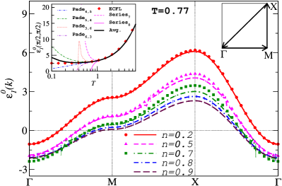
Figure 1: (Color online) The first symmetric moment $\varepsilon_{1}^{0}(k)$ at $T=0.77$ vs momentum around the irreducible wedge of the Brillouin zone (the path is shown in the right inset). Lines are results from the series and symbols for $n\leq 0.7$ are from ECFL calculations. Left inset: $\varepsilon_{1}^{0}(k)$ for $n=0.2$ at $k=(\pi/2,\pi/2)$ from the ECFL (diamonds), up to orders seven and eight of the series (labeled Series₇ and Series₈), and up to the eighth order after various Padé approximations, vs temperature on a logarithmic scale. The numbers in the subscripts of “Padé” labels represent the order of the polynomial in the numerator and in the denominator of the Padé ratio, respectively. “Avg.” denotes the average between Padé_{4,5} and Padé_{5,4}. In the main panel, the results for the series are either the average between Padé_{4,5} and Padé_{5,4} or Padé_{5,5} and Padé_{5,4}, pade with the “error bars” defined as the differences between the two. errorbars

In Fig. 1, we plot the symmetric first moment $\varepsilon_{1}^{0}(k)$ as a function of momentum at $T=0.77$ for five different densities $n=0.2$, 0.5, 0.7, 0.8, and 0.9. We find excellent agreement between the results from the series and the ECFL for $n=0.2$ for all the momenta around the irreducible wedge of the Brillouin zone. At higher densities up to $n=0.7$ (beyond which the ECFL results are not quoted), the agreement is still very good, except around the zone corner, where the disagreement grows as the density increases. shift The results for the series are obtained from Padé approximations as the bare results show divergent behavior at $T<1$. The number of terms in the series is large enough to justify the utilization of Padé approximations in order to extend the convergence to lower temperatures. A comparison of several of these approximations with the ECFL results for a (low) density of $n=0.2$ is shown in the inset of Fig. 1. In that case, we see that the agreement between the two methods extends to temperatures as low as $T=0.3$ using Padé approximations.

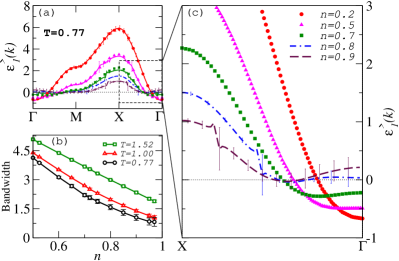
Figure 2: (Color online) (a) The first greater moment $\varepsilon_{1}^{>}(k)$ at $T=0.77$ vs momentum for the same path around the irreducible wedge of the Brillouin zone as in Fig. 1. Lines and symbols are also the same as in Fig. 1. (b) The bandwidth of $\varepsilon_{1}^{>}(k)$, defined as the difference between its maximum and minimum values at momenta shown in panel (a), vs density for $T=1.52,1.00$, and $0.77$. Panel (c) zooms in the results in panel (a) for $k$ along the nodal direction. The two methods more or less agree with each other, within the error bars, in this window for $n\leq 0.7$, and therefore, we show only the ECFL results for the latter cases.

The greater moment $\varepsilon_{1}^{>}(k)$ is plotted in Fig. 2(a) at the same temperature and densities as in Fig. 1. For $\varepsilon_{1}^{>}(k)$, the overall agreement between the series expansions and the ECFL results for all $n\leq 0.7$ is better than for $\varepsilon_{1}^{0}(k)$, especially around the $X$ point. We also note that $\varepsilon_{1}^{>}(k)$ exhibits a more intriguing behavior than $\varepsilon_{1}^{0}(k)$. One of the prominent features of the former, seen in Fig. 2(a), is the significant narrowing of the band by increasing the density. In Fig. 2(b), we plot the bandwidth [i.e., $\max(\varepsilon^{>}_{1})-\min(\varepsilon^{>}_{1})$] from the series as a function of density at $T=1.52$, 1.00, and 0.77. It appears that the bandwidth deviates from a linear dependence on $n$ by decreasing the temperature, and saturates for $n\to 1$ at a nonzero value that decreases towards zero with decreasing $T$. Close to $n=1$ at $T=0.77$, we find a weaker agreement between different Padé approximations, leading to larger error bars. The version of ECFL in Ref. (hansen-shastry, ) cannot be used to study this effect as the high-density region $n\sim 1$ is beyond its regime of validity.

Another interesting feature of $\varepsilon_{1}^{>}(k)$ [Fig. 2(a)] is the change in sign of its slope near the $\Gamma$ point as the density increases towards unity. To better study this feature, in Fig. 2(c), we report only the results along the nodal direction. We find that for $n\gtrsim 0.7$, the greater moment initially decreases as the momentum increases from zero, leading to a negative curvature, or effective mass, at the $\Gamma$ point. This feature becomes more pronounced as we increase the density, or decrease the temperature (see Fig. 3). These results hint at a possible reconstruction of the Fermi surface, i.e., the negative mass persisting and extending in $k$ space so as to reach the Fermi momentum. The appearance of such a hole pocket in the (hole) underdoped regime, could be of interest in ARPES and quantum oscillation studies. However, establishing this firmly requires higher order terms in the series, and is therefore difficult.

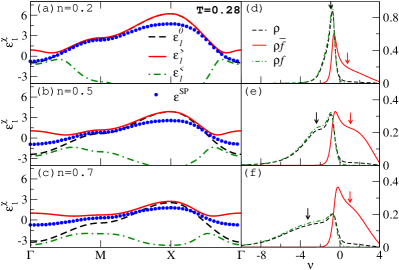
Figure 3: (Color online) Comparison of the SP location $\varepsilon^{\textrm{SP}}(k)$ (symbols) and the three moments from ECFL at $T=0.28$ and for (a) $n=0.2$, (b) $n=0.5$, and (c) $n=0.7$. Right panels show the corresponding spectral functions and their products to $\bar{f}(\omega)$ and $f(\omega)$ at $\Gamma$ for the same densities shown in the left panels. Dark (Light) arrows show the values of $\varepsilon_{1}^{0}$ ($\varepsilon_{1}^{>}$). At low densities, the SP location is estimated well by the first symmetric moment. At higher density, the spectral function is skewed and the greater moment, which is calculated for the spectral function after most of its weight in the negative frequency region is cut off, provides a better estimate.

So far, we have seen that for intermediate temperatures and at relatively small densities, the ECFL agrees extremely well with the results of the series expansion. But, unlike the series expansion, ECFL is not limited to high temperatures at those densities and can be used to study the moments, and more importantly, the real-frequency spectral functions, at much lower temperatures. Therefore, we focus on the ECFL results at $n=0.2$, 0.5, and 0.7, and at a reduced temperature of $T=0.28$, a temperature at which the series do not converge. In Figs. 3(a)-3(c), we plot $\varepsilon_{1}^{0}(k)$, $\varepsilon_{1}^{>}(k)$, and $\varepsilon_{1}^{<}(k)$ from the ECFL, along with $\varepsilon^{\textrm{SP}}(k)$, obtained from the spectral functions, at different momenta. We find that in the physically interesting region of low temperatures and high densities, where correlation effects are strongest, the location of the SP is generally better estimated by the greater moment than by the symmetric, or the lesser one [see Fig. 3(c)].

The spectral functions shown in Figs. 3(d)-3(f) help us understand why this is the case. There, we plot the spectral functions $\rho_{{\cal{G}}}(k,\omega)$, $\rho_{{\cal{G}}}(k,\omega)\bar{f}(\omega)$, and $\rho_{{\cal{G}}}(k,\omega)f(\omega)$, corresponding to the three moments at $k=(0,0)$, where the differences between the moments are the most pronounced, vs frequency. At $n=0.2$, there exists a relatively sharp quasiparticle peak in $\rho_{{\cal{G}}}$ whose location matches the first symmetric moment (marked by a dark arrow) very well. $\varepsilon_{1}^{>}(k)$, on the other hand, falls slightly to the right of the quasiparticle peak (marked by a light-colored arrow) as most of the spectral weight in negative frequencies is cut off after multiplying $\rho_{{\cal{G}}}$ by $\bar{f}(\omega)$ [see Eq. (5)]. Also, since there is very little spectral weight in the positive frequency side, $\varepsilon_{1}^{<}(k)$ is very close in value to $\varepsilon_{1}^{0}(k)$. As the density is increased to $n=0.5$, the spectral function is skewed as a result of correlations. In this case, at small $k$, there is much more spectral weight on the left of the SP than on the right, causing the symmetric moment to be smaller than $\varepsilon^{\textrm{SP}}(k)$. This feature becomes more significant at a higher density of $n=0.7$, where almost all of the spectral weight is in the negative frequency side. As a result, multiplying $\rho_{{\cal{G}}}$ by $\bar{f}(\omega)$ helps in neglecting the excess weight on the left side of the SP. Hence, $\varepsilon_{1}^{>}(k)$, which is readily available from the series at even higher densities, may be used as an indicator of $\varepsilon^{\textrm{SP}}(k)$ using this insight from the ECFL spectra.

IV Summary

We employ two complementary methods, namely, a strong-coupling series expansion and the ECFL, to calculate the moments of the spectral functions for the infinite-$U$ Hubbard model. Unveiling the basic physics of the model is benefited by the complementarity of those approaches. Furthermore, the series expansion results provide the first independent check of the ECFL theory, which has been self-consistently established. At intermediate temperatures and low densities, where the results from both methods are available, we find very good agreement between the two. Unlike ECFL, the series is not limited to small densities and, by increasing the density in the series to near half filling, we find interesting features in the dispersion of the moment with dominant contributions from unoccupied states (the greater moment). These include a significant narrowing of its band as well as hints of Fermi-surface reconstruction. Unlike the series, the ECFL is not limited to high temperatures and, by exploring the ECFL results at lower temperatures, we find that the greater moment better describes the location of the SP as the density increases. This is understood based on the skewing of the spectral functions in the negative frequency region in the strongly-correlated regime.

V Acknowledgments

This work was supported by DOE under Grant No. FG02-06ER46319 (B.S.S., D.H., and E.P.), and by NSF under Grant No. OCI-0904597 (E.K. and M.R.).

References

- (1) H. Mori, Prog. Theor. Phys. 33, 423 (1965); 34, 399 (1965); M. Dupuis, ibid. 37, 502 (1967); K. Tomita and H. Mashiyama, ibid. 51, 1312 (1974).
- (2) W. Nolting, Z. Phys. 255, 25 (1972); J. J. Deisz, D. W. Hess, and J. W. Serene, Phys. Rev. B 66, 014539 (2002).
- (3) Phase Transitions and Critical Phenomena, edited by C. Domb and M. S. Green (Academic, London, 1974), Vol. 3.
- (4) W. Brauneck, Z. Phys. B 28, 291 (1977); K. Kubo, Prog. Theor. Phys. 64, 758 (1980); R. R. P. Singh and R. L. Glenister, Phys. Rev. B 46, 14313 (1992); 46, 11871 (1992); W. O. Putikka, M. U. Luchini, and T. M. Rice, Phys. Rev. Lett. 68, 538 (1992); W. O. Putikka, M. U. Luchini, and R. R. P. Singh, ibid. 81, 2966 (1998).
- (5) G.-H. Gweon, B. S. Shastry, and G. D. Gu, Phys. Rev. Letts 107, 056404 (2011); K. Matsuyama, G. H. Gweon, arXiv:1212.0299 (unpublished).
- (6) T. Valla, A. V. Fedorov, P. D. Johnson, B. O. Wells, S. L. Hulbert, Q. Li, G. D. Gu, N. Koshizuka, Science 285, 2110 (1999).
- (7) C. G. Olson et al., Phys. Rev. B 42, 381 (1990), T. Yoshida et al., J. Phys. Condens. Matter 19, 125209 (2007).
- (8) A. Kaminski et al., Phys. Rev. B 69, 212509 (2004)
- (9) B. S. Shastry, Phys. Rev. Lett. 107, 056403 (2011); 108, 029702 (2012); Phys. Rev. B 84, 165112 (2011); 87, 125124 (2013); Phys. Rev. Lett. 109, 067004 (2012); Phys. Rev. B 81, 045121 (2010).
- (10) D. Hansen and B. S. Shastry, arXiv:1211.0594 (unpublished).
- (11) E. Khatami, E. Perepelitsky, B. S. Shastry, and M. Rigol (unpublished).
- (12) A. A. Abrikosov, L. Gorkov and I. Dzyaloshinski, Methods of Quantum Field Theory in Statistical Physics, (Prentice-Hall, Englewood Cliffs, NJ, 1963).
- (13) E. Perepelitsky and B. S. Shastry (unpublished).
- (14) W. Metzner, Phys. Rev. B 43, 8549 (1991).
- (15) B. Farid, Philos. Mag. 84, No. 9, 909 (2004).
- (16) Note that the zeroth order terms in the expansion for is proportional to . Hence, Padé{l,m} with will match the series order by order exactly up to the eighth order. Nevertheless, we find that Padé{5,5}, for which one assumes that the coefficient of the ninth order term in the series is zero, often results in less spurious features than with Padé{4,5}, and therefore is used instead of the latter for and . On the other hand, since is itself a ratio of two polynomials, either of the above two Padé approximants is equally valid. In this case (Fig. 2), we use the average of Padé{5,4} and Padé{5,5} for and Padé{5,4} and Padé{4,5} for the rest.
- (17) There is no error per se in the calculation of the coefficients of terms in the series. The so-called error bars are merely a measure of the convergence limit for the Padé approximations at low temperatures, where the bare results show divergent behavior. They do not represent statistical or particular systematic errors.
- (18) We may take the curves of , or more accurately, as estimates of the SP dispersion , after shifting them by a constant chosen to pass them through zero energy at the Fermi momentum (as in Figs. 1 and 2). The magnitudes of the shift constants are on the scale seen in Figs. 3(d)-3(f) as the separation between the peak locating the and the arrows locating the moments.