The Pan-STARRS 1 Photometric Reference Ladder, Release 12.01

Abstract

As of 2012 Jan 21, the Pan-STARRS 1 $3\pi$ Survey has observed the 3/4 of the sky visible from Hawaii with a minimum of 2 and mean of 7.6 observations in 5 filters, $g_{\rm P1}$,$r_{\rm P1}$,$i_{\rm P1}$,$z_{\rm P1}$,$y_{\rm P1}$. Now at the end of the second year of the mission, we are in a position to make an initial public release of a portion of this unprecedented dataset. This article describes the PS1 Photometric Ladder, Release 12.01 This is the first of a series of data releases to be generated as the survey coverage increases and the data analysis improves. The Photometric Ladder has rungs every hour in RA and at 4 intervals in declination. We will release updates with increased area coverage (more rungs) from the latest dataset until the PS1 survey and the final re-reduction are completed. The currently released catalog presents photometry of $\sim 1000$ objects per square degree in the rungs of the ladder. Saturation occurs at $g_{\rm P1},r_{\rm P1},i_{\rm P1}\sim 13.5$; $z_{\rm P1}\sim 13.0$; and $y_{\rm P1}\sim 12.0$. Photometry is provided for stars down to $g_{\rm P1},r_{\rm P1},i_{\rm P1}\sim 19.1$ in the AB system. This data release depends on the rigid ‘Ubercal’ photometric calibration using only the photometric nights, with systematic uncertainties of (8.0, 7.0, 9.0, 10.7, 12.4) millimags in ($g_{\rm P1}$,$r_{\rm P1}$,$i_{\rm P1}$,$z_{\rm P1}$,$y_{\rm P1}$). Areas covered only with lower quality nights are also included, and have been tied to the Ubercal solution via relative photometry; photometric accuracy of the non-photometric regions is lower and should be used with caution.

1. INTRODUCTION

Accurate photometry is one of the key tools of astronomy, yet ground-base astronomy continues to suffer the traditional challenge of accurate photometric calibration. Careful analysis of standard ground-based CCD imaging data can yield relative photometry of objects in a small field with accuracy of 1% or better, and exotic techniques can produce much higher accuracy in special cases (e.g., Tonry et al., 2005; Johnson et al., 2009). The remaining challenge for the generic astronomer is that of calibration of the photometry of a given field into one of the standard systems.

Part of the difficulty comes from the various effective bandpasses due to the different telescopes and cameras used by observers. Critical attention must be paid to the bandpass defined by the choice of filter, detector, etc (see, e.g. Bessel, 1990). However, for main sequence stars of spectral types earlier than $\sim$ K0, these bandpass effects can be dealt with through measured color transformations. The larger challenge comes from the calibration of the images with respect to a well-defined reference.

Calibration of images obtained from the ground is naturally difficult due to the large area of the sky and the small sizes of detectors, even modern large mosaic cameras. Calibration of most individual images still ultimately relies on observations of objects in reference fields outside of the field of view of interest. Since there is currently no all-sky network of calibrated references with sufficiently dense spacing, the calibration observations invariably do not overlap the science fields. Photometric calibration is thus sensitive to the systematic impact of changes in the atmosphere or the instrument between the observation of the science field and the reference field.

Ground-based optical astronomy is on the verge of escaping this traditional problem – several projects are now (or will soon be) able to define dense large-area networks of reference photometry with accuracies at or below the 1% level. The Sloan Digital Sky Survey (York et al., 2000), for example, provides good photometry across the $1.4\pi$ steradians covered by that survey (up through DR9), with reported systematic errors of $\sim 10$ millimagnitudes for the $g,r,i,z$ filters (Padmanabhan et al., 2008). LSST will eventually provide the same or better for the $>2\pi$ steradians of the portion of the sky covered by that survey.

The Pan-STARRS 1 project is surveying the $3\pi$ steradians north of $-30$ deg declination Chambers et al. (in prep). A major goal of this survey project is the construction of a precision photometry reference catalog covering the entire $3\pi$ region. The design of the survey and the careful attention to calibration concerns place it in an excellent position to provide a photometric (and astrometric) reference for this entire $3\pi$ region. The Pan-STARRS 1 Survey is continuing, and final calibration will not be complete for $\sim$ 6 months after the survey completion, roughly mid 2014. At this point in time, however, interest in the community has grown strong in a preliminary data release to demonstrate the progress at precision photometric calibration, and to potentially provide reference data in the PS1 photometry system, and in regions not currently served by the SDSS survey.

2. Pan-STARRS1

Table 1Pan-STARRS 1 $3\pi$ Survey Coverage Statistics

	Image coverage1			50%	Exposure Coverage3
Filter	95%	50%	5%	Det2	3∘ FOV	3.3∘ FOV
$g_{\rm P1}$	1.14	4.76	9.12	3.93	5.77	6.98
$r_{\rm P1}$	1.06	4.48	9.15	3.70	5.63	6.81
$i_{\rm P1}$	1.13	4.81	9.31	3.97	5.85	7.08
$z_{\rm P1}$	2.61	6.24	10.95	5.15	7.29	8.83
$y_{\rm P1}$	2.92	6.37	10.50	5.28	7.43	8.99

¹(95,50,5)% of the $3\pi$ Survey region is covered by the given number of images as of 2011 Jan 21.
²Interpolated Median number of detections per filter for bright sources
³Mean coverage expected for a filled circular focal plane with the given diameter

The 1.8m Pan-STARRS 1 telescope, located on the summit of Haleakala on the island of Maui in the Hawaiian island chain, has been performing a set of astronomical surveys since May 2010. The long-term goals of the Pan-STARRS project include the construction of a four telescope system (Kaiser et al. 2002) on Mauna Kea; the Pan-STARRS 1 telescope, analysis, and data publication system Kaiser et al. (2010) are prototypes of the full hardware and software systems required for the 4 telescope array. Pan-STARRS 1 is currently being operated full-time in survey mode, with several intertwined programs. The surveys are designed around a wide-ranging set of science drivers, addressing astronomical issues as diverse as the contents of the inner solar system (Hsieh et al., 2012, e.g., the discovery of the main belt comet Comet P/2006 VW139) to galaxy clustering and cosmology using Type Ia supernovae (e.g., Narayan et al., 2011).

The wide-field optical design of the Pan-STARRS 1 telescope (Hodapp et al., 2004), based on a 1.8 meter diameter $f$/4.4 primary mirror and an 0.9 m secondary, produces a 3.3 degree field of view with low distortion and minimal vignetting even at the edges of the illuminated region. The optics, in combination with the natural seeing, result in generally good image quality: 75% of the images have full-width half-max values less than (1.51, 1.39, 1.34, 1.27, 1.21) arcseconds for ($g_{\rm P1}$,$r_{\rm P1}$,$i_{\rm P1}$,$z_{\rm P1}$,$y_{\rm P1}$), with a floor of $\sim 0.7$ arcseconds. The Pan-STARRS 1 camera (Tonry & Onaka, 2009) consists of a mosaic of 60 edge-abutted $4800\times 4800$ pixel detectors, with 10 $\mu$m pixels subtending 0.258 arcsec. The detectors are back-illuminated CCDs manufactured by Lincoln Laboratory and are read out using a StarGrasp CCD controller, with a readout time of 7 seconds for a full unbinned image. Initial performance assessments are presented in Onaka et al. (2008). The active, usable pixels cover $\sim 80$% of the FOV. Routine observations are conducted remotely from the Advanced Technology Research Center in Kula, the main facility of the University of Hawaii’s Institute for Astronomy operations on Maui.

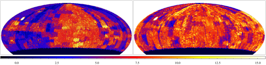
Figure 1.— Plots of the sky coverage of the $3\pi$ Survey through 21 Jan 2012. The color (greyscale in print version) shows the number of separate exposures overlapping the given location, as indicated by the scale. The left panel shows the distribution for $g_{\rm P1}$ while the right panel shows the distribution for $y_{\rm P1}$. The distributions for $r_{\rm P1}$ & $i_{\rm P1}$ are similar to $g_{\rm P1}$, while that of $z_{\rm P1}$ mimics $y_{\rm P1}$. RA = 0.0 is at the center of the plots and increases to the left. The patch at $09^{h}15^{m},+30\hbox{${}^{\circ}$}45\arcmin$ was observed with the full set of $3\pi$ exposures in 2010 Feb as a demonstration dataset.

Images obtained by the Pan-STARRS 1 system are saved and processed on a dedicated data analysis cluster located at the Maui High Performance Computer Center in Kihei, Maui. Observations are automatically processed in real time by the Pan-STARRS 1 Image Processing Pipeline (IPP, Magnier, 2006), with the ultimate goals being the 1) characterization of astronomical objects in the individual images; 2) construction of stacks of multiple images of the same areas of the sky to improve the sensitivity and to fill in gaps (along with the characterization of the objects in those stacks); 3) construction of difference images between individual images or stacks and reference images from another epoch for the purpose of detecting variable and moving objects. This article relies only on data from the analysis of the individual exposures, not on any of the stacked or difference images.

In more detail, individual images are detrended: non-linearity and bias corrections are applied, a dark current model is subtracted and flat-field corrections are applied. The $y_{\rm P1}$-band images are also corrected for fringing: a master fringe pattern is scaled to match the observed fringing and subtracted. Mask and variance image arrays are generated with the detrend analysis and carried forward at each stage of the IPP processing. Source detection and photometry are performed for each chip independently. Astrometric and photometric calibrations are performed for all chips together in a single exposure.

For the first 20 months, lacking all-sky photometry in the Pan-STARRS1 band-passes, a provisional photometric calibration was performed on the nightly exposures using a synthetic photometric catalog based on the combined fluxes in Tycho, USNO-B, and 2MASS. In practice, since Tycho only contributes very bright stars, and the large photometric errors for USNO stars mean they carry little weight, these calibrations are effectively tied to 2MASS as if all stars were on the main sequence color locus. The resulting photometric calibrations are observed to be no better than $\sim 5$%.

Global re-calibration analysis of the photometric Pan-STARRS 1 data, as discussed in more detail below, has been used to generate a PS1-based reference catalog which is now used for nightly science photometric calibration (Schlafly et al., 2012). This reference catalog also uses the internally improved relative astrometric calibration for improved accuracy of the astrometry.

2.1. The Pan-STARRS 1  $3\pi$ Survey

The PS1 telescope is operated by the PS1 Science Consortium to perform a set of inter-twined surveys with a range of spatial and temporal coverage. Several narrow-field “Medium Deep” surveys are complemented by the wide-area $3\pi$ Survey, the latter allocated 56% of the available observing time. The $3\pi$ Survey aims to observe the portion of the sky North of $-30$ deg declination, with a total of 20 exposures per year in all filters for each field center. The $3\pi$ Survey observations are performed with extensive dithering between different exposures so that the overlaps can be used to tie down the photometric and astrometric system.

The $3\pi$ Survey observations are performed using the five main filters ($g_{\rm P1}$,$r_{\rm P1}$,$i_{\rm P1}$,$z_{\rm P1}$,$y_{\rm P1}$). Details of the passband shapes are provided by Tonry et al. (2012). Provisional response functions (including 1.2 airmasses of atmosphere) are available at the project’s web site. The full survey strategy is described in Chambers et al. (in prep); we summarize the salient details below.

2.1.1 Observing Strategy

The $3\pi$ Survey observations are performed on a complex schedule in order to balance the needs of the different survey science projects. The goal is to obtain a total of 12 observations in each filter for any spot in the observable region by the end of the survey mission. This goal actually refers to a theoretical survey with a perfectly filled focal plane with no gaps or overlaps between neighboring observations. In practice, gaps in the focal plane (between cells, between chips, and from masked pixels) result in a fill-factor of $\sim 80$% for a single exposure. Neighboring exposures have both overlapping areas as well as gaps between the exposure due to the layout of the chips in the camera. The net effect of the overlaps and incomplete fill factor is illustrated in Table 1, discussed in more detail below. While the goal is to achieve the full $3\pi$ coverage in 3 years of observations, it is expected that an additional 6 - 12 months of cleanup observations will be needed to fill in holes due to weather and other down-time, and to improve the homogeneity of the full survey.

The temporal distribution of the 12 observations per filter is somewhat complicated. The following guidelines are used by the observing system, though some observations will inevitably fail to meet these goals. First, any specific field is always observed 2 times in a single night in a single filter, nominally within 20 - 30 minutes. This so-called “Transient Time Interval” allow for the discovery of moving objects (asteroids and NEOs); as part of the nightly processing these “TTI-pairs” are mutually subtracted and objects detected in the difference image are reported to the Moving Object Pipeline Software (MOPS). Second, the blue bands ($g_{\rm P1}$, $r_{\rm P1}$, $i_{\rm P1}$) are observed close to opposition to enable asteroid discovery. These observations normally occur within $\sim 1.5$ months of opposition for any given field. Thus any given field should be observed a total of 12 times in these 3 filters within a 2-3 month window each year. For the reddest 2 bands ($z_{\rm P1}$ & $y_{\rm P1}$), the observations are scheduled as far from opposition as feasible in order to enhance the parallax factors and allow for discovery of faint, low-mass objects in the solar neighborhood. This constraint results in 2 observations in each of $z_{\rm P1}$ & $y_{\rm P1}$ occurring roughly 4-6 months before and 4-6 months after opposition for any given field.

The pointing of individual observations is designed to trade off between maximal overlaps and optimized image differencing. The TTI pair images are, as much as possible, obtained in the same pointing, both location of the boresight and rotation on the sky, in order to minimize the loss of area in the difference image from mis-matched gaps. Subsequent sets of TTI pairs are obtained at offset positions to tile over the boundaries between neighboring exposures. A set of telescope pointings are defined to carefully cover the entire $3\pi$ region with a judicious balance between the total number of exposures and the total area missed due to gaps between the exposures. One set of these telescope pointings is called a “$3\pi$ tessellation”. The base tessellation is used for the first TTI pair of observations. Subsequent observations follow a $3\pi$ tessellation offset from the base by Euler angle rotations which shift most of the boresights by $\sim 50\%$ of the field diameter. Note that no single pair of tessellations can have all field centers offset by a fixed amount; for any pair of tessellations, some subset of boresight positions will have only small offsets. By choosing different poles for these rotations, all fields can have most observations with substantial offsets.

The end result of the scheduling and dithering strategy is that the full $3\pi$ region is covered in a wide range of time periods in each filter and has a large range of spatial overlaps. These overlaps provide a tight mesh for any global photometric and astrometric solution, while the temporal coverage increases the chances that all areas receive photometric observations, or are at least not too distant from photometric data.

2.1.2 Survey Coverage to Date

The scheduling constraints described above, when coupled with vagaries of weather, the need to avoid the moon, and the other (non-3$\pi$) survey observations make the actual scheduling of the observations quite challenging. The overall observing strategy on a nightly basis is to start and end the nights with $z_{\rm P1}$ or $y_{\rm P1}$ observations and to schedule the $g_{\rm P1}$, $r_{\rm P1}$ and $i_{\rm P1}$ observations for the hours near midnight. The 3$\pi$ observation blocks are interspersed with observations for the other survey components (e.g., Medium Deep fields). In addition, as the lunation progresses, the amount of time used for the red or blue bands is shifted as the sky brightness increases. In general, observations are obtained fairly close to the Meridian: for observations away from the zenith keyhole, the hour-angle distribution is Gaussian with $\sigma\sim 1$ hour.

Figure 1 illustrates the spatial coverage of the $3\pi$ Survey to date (2012/01/21). The left panel shows the density of coverage for $g_{\rm P1}$, while the right panel shows the density of coverage for $y_{\rm P1}$. The blue bands ($g_{\rm P1}$, $r_{\rm P1}$, $i_{\rm P1}$) have generally similar coverage, as do the two red bands. To date, the blue bands have been somewhat more affected by weather. The median coverage for any point in the $3\pi$ region is between 4.5 and 6.3 exposures, depending on the band. With $\sim 5$ exposures on average in $\sim 1.5$ years of survey operations, we are generally on track to achieve 12 visits by the end of the 3.5 year mission. However, while some effort is being made in the second half of the survey to fill in gaps due to the weather, the final coverage will likely not be extremely uniform. The top-level goal is to obtain photometric observations for all areas in all filters, though this will be challenging.

These coverage numbers are defined based on the overlap of chip boundaries for those chips actually loaded into the photometry database. The median coverage in the $3\pi$ region is defined as the number of chips covering 50% of patches in the full $3\pi$ region. Table 1 lists the median coverage for each filter as well as the 5% and 95% coverage values. Since there are dead spaces in chips (gaps between cells and masked pixels), the number of detections for a well-measured star will be somewhat less than the number of overlapping images. This effect is reflected in the 5th column of Table 1, which gives the median number of detections for moderately bright (S/N $\sim$ 50) objects. The last two columns of the table give the expected coverage of the full $3\pi$ region (down to Dec of -32^∘, where we have partial coverage), if PS1 had a completely filled circular focal plane with field of view 3.0 and 3.3^∘.

The database includes measurements with all quality levels. The data processing version used for this analysis has suffered from a relatively high rate of artifacts (false positive detections), either due to instrumental structures, optical features such as ghosts and diffraction spikes, and background subtraction failures. Since January 2012, the image processing team have made substantial improvements in reducing these sources of false positives, and in flagging the artifacts which remain. However, the data used in this work have not yet had the benefit of these improvements. For the purposes of this article, we can robustly filter out these false detections by requiring multiple observations of the same object and by restricting our attention to brighter objects. The database used for this analysis contains $3.03\times 10^{10}$ measurements of $2.2\times 10^{9}$ objects at all magnitudes; including only those objects with 3 or more detections, the dataset includes $2.66\times 10^{10}$ detections of $1.49\times 10^{9}$ objects.

2.1.3 Overall System Zero Points

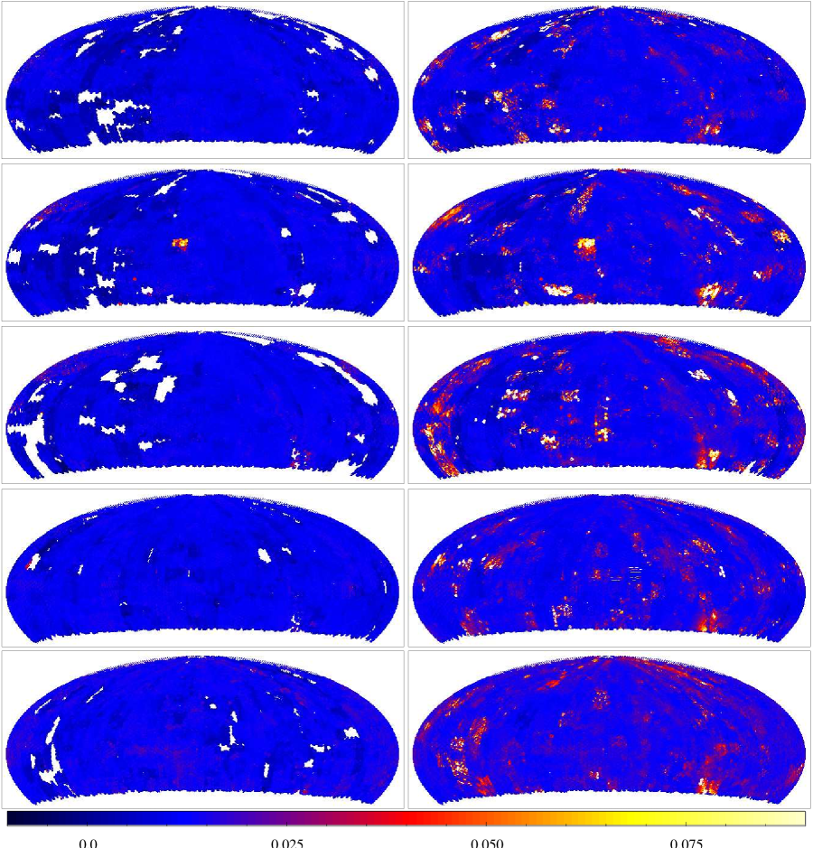
Figure 2.— Plots of the scatter for bright stars using just Ubercal data (left) or all PS1 measurements (right). The color scale shows the amplitude of the scatter in magnitudes. RA = 0.0 is at the center of the plots and increases to the left.

Traditional astronomical magnitudes, such as the Johnson-Kron-Cousins $UBVRI$ system, have been defined as 2.5 times the logarithm of the ratio of fluxes between the object of interest as observed with the given telescope to that of the star Vega observed with the same instrumentation. Some of the drawbacks of this system include (1) a strong dependence on the quality of our knowledge of the magnitudes of Vega in any bandpass of interest and (2) the difficulty of observing one of the brightest stars in the sky with the same instrument used to observe some of the faintest objects known.

Pan-STARRS 1 uses the alternative “AB magnitude system”, introduced by Oke & Gunn 1983, in which the magnitude of an object is defined by the integral of the flux density spectrum multiplied by the overall system throughput as a function of wavelength for the telescope of interest. Symbolically, for a telescope with a system response of $A(\nu)$ and an object with a flux density spectrum of $f_{\nu}$ (erg/sec/cm²/Hz), the AB magnitude for a band-pass is defined to be:

$$m_{AB}=-2.5\log\frac{\int f_{\nu}(h\nu)^{-1}A(\nu)d\nu}{\int 3631\mbox{Jy}(h\nu)^{-1}A(\nu)d\nu}$$ (1)

While this system is not subject to the drawbacks suffered by the Vega system, it has difficulties of its own. In particular, the accuracy of the calibration for any given telescope is limited by (1) our knowledge of the system response (including the atmosphere!) and (2) our knowledge of the spectral energy distribution of a specific star of interest. In practice, like the Vega system, broad-band magnitudes are defined by comparison with the observed magnitudes of well-known stars. Since stars with spectral types earlier than $\sim$ early K are predominantly a continuum source with minor absorption lines, the broad-band colors of stars vary smoothly. Unlike traditional Vega-based photometry, however, in the AB system stars of colors different from the spectrophotometric reference have well-defined magnitudes as long as the bandpass is well measured.

Tonry et al. (2012) have determined the overall system zero points necessary to place the Pan-STARRS 1 magnitudes onto the AB system. We summarize the details of that analysis here.

First, they have determined the relative spectral response of the Pan-STARRS 1 system from the top of the telescope to the detector, in the absence of filters, using a tunable laser and a NIST-calibrated photodiode. To do this, the light from the tunable laser was used to illuminate both the pupil of the telescope and the photodiode. The GPC1 camera was used to record the flux from the laser after it had passed though the full optical system, with the filter holder in the ‘open’ slot. A sequence of measurements was made for 2nm steps from 400 nm to 1100nm, and the flux observed by the calibrated photodiode compared to the flux observed by GPC1. The resulting scans defined the relative response of the system as a function of wavelength without the filters.

The filter transmission curves were measured by the manufacturer, Barr Precision Optics, at a number of positions and angles of incidence. Tonry et al. (2012) also measured the filter curves including the filter in the beam and running the tunable laser + diode system described above. The two sets of data agree well; in their analysis Tonry et al. (2012) adopt the Barr curves as the reference set.

The third optical element in the PS1 system is the atmosphere above the telescope. Tonry et al. (2012) calculate the transmission of the atmosphere as a function of wavelength with the model atmosphere program MODTRAN (Anderson, G.P., et al., 2001). These data are used to calculate the atmospheric extinction as a function of airmass, precipitable water vapor (PWV), and the power-law slope of a given source SED. The PS1 system has been monitoring the PWV content of the atmosphere since June 2011.

Putting together the above components, Tonry et al. (2012) tie down the overall system zero points by observing a selection of spectrophotometric standards with PS1 in a photometric night. The above components of the spectral response of the system were combined and applied to the reported SEDs of the 7 standards to predict observed PS1 fluxes. In addition, a large number of stars with measured spectra were used to construct PS1 stellar locus diagrams to provide an additional set of constraints. Comparison of the predicted and observed magnitudes in each of the 7 available PS1 filters ($g_{\rm P1}$,$r_{\rm P1}$,$i_{\rm P1}$,$z_{\rm P1}$,$y_{\rm P1}$, $w_{\rm P1}$, and open) led Tonry et al. (2012) to introduce tweaks to 12 system parameters to obtain the best match. These tweaks are all at the $\sim$ 1% level, and are the result of the accuracy achieved in the spectral response measurement.

2.1.4 The Ubercal Analysis

Table 2Bit-flags used to exclude bad or low-quality detections

FLAG NAME	Hex Value	Bad / Poor	Description
PM_SOURCE_MODE_FAIL	0x00000008	Bad	Fit (non-linear) failed (non-converge, off-edge, run to zero)
PM_SOURCE_MODE_POOR	0x00000010	Poor	Fit succeeds, but low-SN or high-Chisq
PM_SOURCE_MODE_PAIR	0x00000020	Poor	Source fitted with a double psf
PM_SOURCE_MODE_SATSTAR	0x00000080	Bad	Source model peak is above saturation
PM_SOURCE_MODE_BLEND	0x00000100	Poor	Source is a blend with other sources
PM_SOURCE_MODE_BADPSF	0x00000400	Bad	Failed to get good estimate of object’s PSF
PM_SOURCE_MODE_DEFECT	0x00000800	Bad	Source is thought to be a defect
PM_SOURCE_MODE_SATURATED	0x00001000	Bad	Source is thought to be saturated pixels (bleed trail)
PM_SOURCE_MODE_CR_LIMIT	0x00002000	Bad	Source has crNsigma above limit
PM_SOURCE_MODE_MOMENTS_FAILURE	0x00008000	Bad	could not measure the moments
PM_SOURCE_MODE_SKY_FAILURE	0x00010000	Bad	could not measure the local sky
PM_SOURCE_MODE_SKYVAR_FAILURE	0x00020000	Bad	could not measure the local sky variance
PM_SOURCE_MODE_BELOW_MOMENTS_SN	0x00040000	Poor	moments not measured due to low S/N
PM_SOURCE_MODE_BLEND_FIT	0x00400000	Poor	source was fitted as a blend
PM_SOURCE_MODE_SIZE_SKIPPED	0x10000000	Bad	size could not be determined
PM_SOURCE_MODE_ON_SPIKE	0x20000000	Poor	peak lands on diffraction spike
PM_SOURCE_MODE_ON_GHOST	0x40000000	Poor	peak lands on ghost or glint
PM_SOURCE_MODE_OFF_CHIP	0x80000000	Poor	peak lands off edge of chip

Schlafly et al. (2012) have reported on the photometric calibration of the first 1.5 years of the PS1 survey. In that analysis (“Ubercal”), the photometric nights are selected and all other data are ignored. Each night is allowed to have a single fitted zero point and a single fitted value for the airmass extinction coefficient per filter (see Eq. 3 below). Zero points of each night are determined by minimizing the dispersion of the measurements of the same stars from multiple nights. Schlafly et al. (2012) also determine flat-field corrections as part of the minimization process. The flat-field corrections are measured for $2\times 2$ sub-regions of each chip in the camera, and are determined by choosing zero point offsets for these patches to minimize the scatter per star. Four distinct time periods (“seasons”) were identified in which these flat-field corrections were quite consistent, but noticeably different from the other seasons. The transitions between the seasons have been identified with specific changes to the optical system: modification of the baffling structures and changes to the collimation and alignment coefficients. The underlying cause of the different flat-fields is believed to be due to small scale changes in the vignetting and PSF structure.

By excluding non-photometric data (both manually up front and iteratively in the analysis) and only fitting 2 additional parameters for each night, the Ubercal solution is both robust and extremely rigid. It is not subject to unexpected drift or sensitivity of the solution to the vagaries of the data set. The Ubercal analysis is also especially aided by the inclusion of multiple Medium Deep field observations every night, helping to tie down overall variations of the system throughput and acting as internal standard star fields. The resulting photometric system is shown by Schlafly et al. (2012) to have reliability across the survey region at the level of (8.0, 7.0, 9.0, 10.7, 12.4) millimags in ($g_{\rm P1}$,$r_{\rm P1}$,$i_{\rm P1}$,$z_{\rm P1}$,$y_{\rm P1}$). In addition, the consistency of the measured zero points (scatter of $\sim 4$ millimag) hints at the possibility of even better overall photometry as more information is used to determine the flat-field variations.

The Ubercal analysis, performing a highly-constrained relative photometry calculation, requires the external definition of the zero point for each filter. Schlafly et al. (2012) set the zero points of their images to match the values resulting from the analysis of Tonry et al. (2012). This is done by matching the photometry of the MD09 Medium Deep field to that measured by Tonry et al. (2012) on the reference photometric night of MJD 55744 (UT 02 July 2011).

2.1.5 Relative Photometry

In this work we have used the Ubercal solution as a starting point, and have used relative photometry between individual exposures to determine the zero points for the data not calibrated by the Ubercal analysis. The combination of overlaps and the rigid base of the Ubercal analysis allows us to determine reliable photometry for areas which were excluded by Schlafly et al. (2012).

The basic analysis is similar in many respects to the Ubercal approach. We start with a database of all observations, using the Pan-STARRS Desktop Virtual Observatory software (DVO, Magnier, 2006). The database links the table of individual ‘detections’ to the images from which they came, and groups the detections into unique astronomical ‘objects’.

Individual detections are characterized by a total number of counts observed for the source, and converted to an instrumental magnitude: $m^{inst}=-2.5\log_{10}(\mbox{counts})+2.5\log(\mbox{exptime})$. The detected objects (at least those which are not detectably variable) have an intrinsic mean magnitude in the AB photometric system, $m^{AB}$, of which each detection is a realization. The instrumental magnitude and the mean magnitude are related by an arithmetic offset which accounts for various effects (zero point, instrumental variations, atmospheric attenuation):

$$m^{AB}=m^{inst}+Z$$ (2)

We can decompose the zero point $Z$ into the primary contributors as follows:

$$Z_{i,n}=a_{n}-k_{n}x_{i}+C_{n}*\mbox{color}+T_{i}$$ (3)

, where $a_{n}$ and $k_{n}$ are the system zero point and trend with airmass for a given period of time, while $x_{i}$ is the airmass ($\sec z$, for zenith angle $z$) of a given image $i$. We also allow for a trend that depends on the color of a star and an additional term measuring any additional reduction in the transparency, $T_{i}$ for any given image (e.g., clouds or haze).

In our analysis, we are taking the system zero point and the mean airmass extinction coefficients provided by the Ubercal analysis, and solving for a single additional offset for each exposure not already tied down by the Ubercal analysis. For this analysis, we neglect the color difference of the different chips, and thus set the value of $C_{n}$ to 0.0. Note that we only use a single mean airmass extinction term for all exposures – the difference between the mean and the specific value for a given night is taken up as an additional element of the atmospheric attenuation.

We minimize the following global $\chi^{2}$ equation by finding the best mean magnitudes for all objects and the best cloud offset for each exposure:

$$\chi^{2}=\sum_{i,j}(m^{inst}_{i,j}+a_{n}-k_{n}x_{i}+T_{i}-m^{sys}_{j})w_{i,j}/\sum_{i,j}w_{i,j}$$ (4)

where $i$ is the index for each image and $j$ is the index for each star. We set the weighting values $w_{i,j}$ to the inverse variance of the individual measurements. If everything were fitted at once and allowed to float, this system of equations would have $N_{images}+N_{stars}\sim 2\times 10^{5}+2\times 10^{9}$ unknowns. We solve the system of equations by iteration, solving first for the best set of mean magnitudes in the assumption of zero clouds, then solving for the clouds implied by the differences from these mean magnitudes. Even with 1-2 magnitudes of extinction, the offsets converge to the milli-magnitude level within 8 iterations.

After a series of 8 initial iterations, we perform outlier rejections. For each star, the inner 50% of measurements are used to define a measurement of the standard deviation which is robust against significant outliers. Using this measurement of the standard deviation, any measurements more than 5$\sigma$ deviant from the median are excluded, and the mean & standard deviation (weighted by the inverse error) are recalculated. The resulting values are used to exclude detections which are more than 3$\sigma$ deviant from the mean. These deviant measurements are then flagged and excluded from the rest of the analysis.

Suspicious images and suspicious stars are also rejected. For the stars, we reject objects with $\chi^{2}_{\nu}$ values more than 20.0, or more than 2$\times$ the median $\chi^{2}_{\nu}$ value, whichever of these cuts is larger. We also reject stars with scatter (standard deviation of the measurements used for the mean) greater than 0.005 mags or 2$\times$ the median scatter, whichever is greater. Similarly for images, we reject those with more than 2 magnitudes of extinction or with scatter greater than 0.075 mags or 2$\times$ the median scatter, whichever is greater. If the star & detection rejection steps have the effect of eliminating too many measurements for a given image, we exclude that entire image. The total number of valid measurements for an image must be $>10$ and the fraction of valid measurements to the total number of measurements considered per image must be $>5\%$.

These cuts are somewhat conservative to limit us to only good measurements. These images and stars are excluded when solving for the system of zero points and mean magnitudes. These cuts are updated several times as the iterations proceed. After the iterations have completed, the poor-quality images are then calibrated based on their overlaps with other images, and mean magnitudes for all stars are calculated.

In this analysis, we use the Ubercal measurements as a rigid base by setting the weight of Ubercal detections to 10x their default (inverse-variance) weight. The calculation of the formal error on the mean magnitudes propagates this additional weight, so that the errors on the Ubercal observations dominates where they are present:

$$\mu=\frac{\sum m_{i}w_{i}\sigma_{i}^{-2}}{\sum w_{i}\sigma_{i}^{-2}}$$ (5)

$$\sigma_{\mu}=\frac{\sum w_{i}^{2}\sigma_{i}^{-2}}{(\sum w_{i}\sigma_{i}^{-2})^{2}}$$ (6)

where $w_{i}$ = 1.0 for non-Ubercal measurements and 10.0 for Ubercal measurements.

In practice, we further restrict the data used in the analysis. We use only the brighter objects, limiting the density to a maximum of 2500 or 3000 objects per square degree (lower in areas where we have more observations). When limiting the density, we prefer objects which are brighter (but not saturated), and those with the most measurements (to ensure better coverage over the available images). We also exclude in advance those measurements for which the photometric analysis flagged the result as suspicious (see Table 2). The latter includes detections which are excessively affected by masks (PSF_QF $<$ 0.85), which land too close to other bright objects, which are suspiciously close to diffraction spikes or ghost images, or which are too close to the detector edges.

We perform the relative photometry analysis on a large area of the sky, but not the entire database, in a given pass. The driver here is to avoid over-filling the memory of our analysis machine (48GB). Another practical consideration is the data I/O needed for a given analysis – processing more, smaller areas costs more time for I/O operations. We have found that we achieve a good balance by splitting the sky into 15 regions: 12 RA bands from -45^∘ to +60^∘, plus the polar region, with the 2 RA bands covering the Galactic Center split in two at Dec = 5^∘. An exposure must be completely contained within an analysis region to have its zero point (cloud offset) determined; images overlapping the edges of the analysis region contribute measurements, but their offsets are held fixed for that analysis region. The analysis regions are defined to have 5 degree overlapping boundaries to ensure that all exposures have the chance to be fitted.

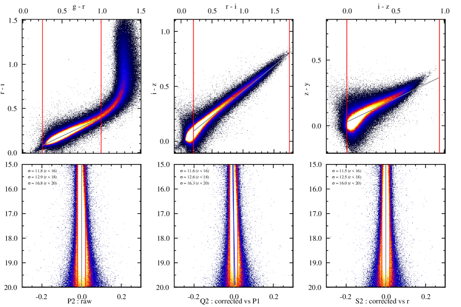
Figure 3.— Demonstration of the stellar locus fitting. Top Row: the 3 2-color planes used for this analysis. The vertical (red) lines mark the range of colors used to define a stellar locus segment for each 2-color plane. The grey line show the initial linear fit to this portion of the stellar locus. Bottom Left: $r_{\rm P1}$ vs the principal color P2 for the $g_{\rm P1}-r_{\rm P1},r_{\rm P1}-i_{\rm P1}$ 2-color plane. Bottom Middle: $r_{\rm P1}$ vs the Q2, the principal color after correction for variation of the stellar locus position as a function of the P1 dimension. Bottom Right: $r_{\rm P1}$ vs the S2, the principal color after correction for variation of the stellar locus position as a function of $r_{\rm P1}$. The inset numbers show the measured scatter for stars with three faint limits. Note the consistent improvement of the scatter for brighter objects.

Once the image zero points & cloud extinctions have been calculated, these values are then applied to the individual measurements and final mean magnitudes are calculated for all objects in the database. Since we are using the reference catalog within the Pan-STARRS project as our internal calibration system, we would like to determine the best set of magnitudes for all objects, regardless of the quality of the data available for each object. Even if we only have poor measurements or no measurements of a given star, we would like to populate the catalog with our best guess given the information available. To this end, we attempt to determine the mean magnitudes in a series of passes. In the first pass, we have a very conservative selection of data to be used for the analysis. In successive passes, we relax our criteria for those objects which had no valid data in the earlier passes. The 5 different levels of data acceptance are:

• pass 0: only ‘good’ measurements as reported by the photometry analysis; reject outliers determined by the relative photometry analysis

• pass 1: accept measurements deemed ‘poor’ by the photometry analysis (‘suspect’, but not ‘bad’ masks; poor fit but not failed fit; etc.)

• pass 2: accept the relative photometry outliers

• pass 3: accept measurements deemed ‘bad’ by the photometry analysis (eg, saturated stars, partially masked detections)

• pass 4: accept 2MASS/Tycho/USNO-based synthetic photometry (see Section 2 above).

For any object in the database, the mean magnitudes in the 5 filters are independently tested for these different levels. Which data quality was used can be determined by examining the flags for that filter.

A final note regarding the use of synthetic photometry: we have found that very bright stars in the PS1 data can be split into multiple measurements by the psphot analysis. In these cases, the synthetic photometry can be more reliable than the PS1 magnitudes. We currently accept the synthetic magnitudes if the implied $3\pi$ Survey magnitude would be severely saturated (instrumental magnitudes $<-15$).

2.1.6 Data Quality Checks

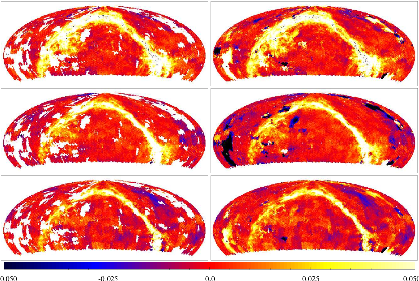
Figure 4.— Plots of the mean offset of the stellar locus for the 3 2-color planes (top-to-bottom: $g_{\rm P1}-r_{\rm P1},r_{\rm P1}-i_{\rm P1}$; $r_{\rm P1}-i_{\rm P1},i_{\rm P1}-z_{\rm P1}$; $i_{\rm P1}-z_{\rm P1},z_{\rm P1}-y_{\rm P1}$). Left column is ubercal data only, right column is all PS1 data. RA = 0.0 is at the center of the plots and increases to the left.

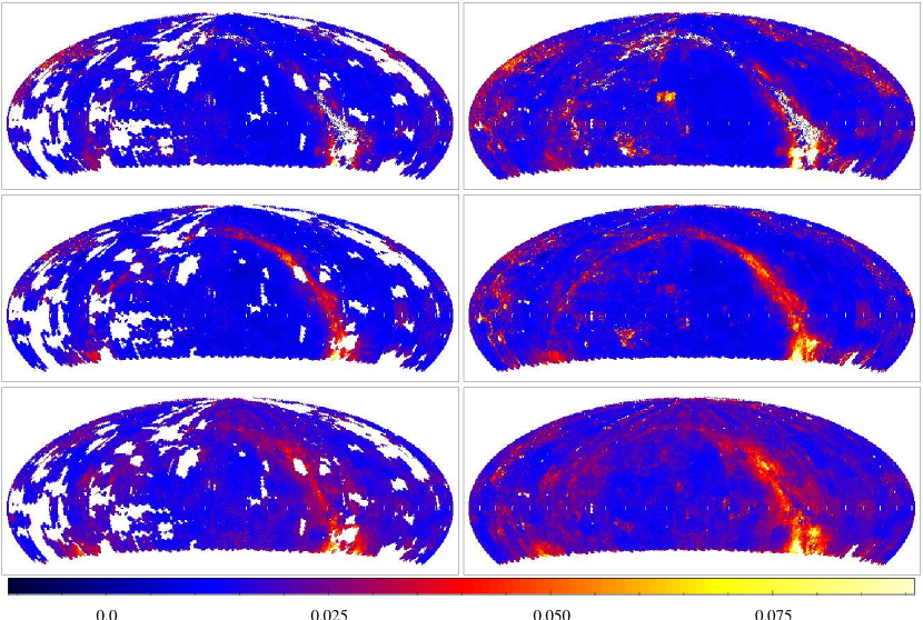
Figure 5.— Plots of the r.m.s. scatter of the stellar locus as a function of position on the sky ($r_{\rm P1}<20.0$) for the 3 2-color planes (top-to-bottom: $g_{\rm P1}-r_{\rm P1},r_{\rm P1}-i_{\rm P1}$; $r_{\rm P1}-i_{\rm P1},i_{\rm P1}-z_{\rm P1}$; $i_{\rm P1}-z_{\rm P1},z_{\rm P1}-y_{\rm P1}$). Left column is ubercal data only, right column is all PS1 data. RA = 0.0 is at the center of the plots and increases to the left.

Figure 2 shows the mean scatter for the measurements of bright stars (instrumental magnitude $<-10$) as a function of position on the sky (one plot for each filter). The left panels show the scatter for only the Ubercal measurements – these plots correspond to the figures in Schlafly et al. (2012), and illustrate the level to which we maintain the photometric quality of the Ubercal analysis. The right-hand panels show the scatter for all PS1 measurements included in the analysis, through (2011-01-21). The scatter is measured by finding the $\pm 1\sigma$ points on the cumulative histogram in the assumption of Gaussian statistics – this makes the measurement insensitive to extreme outliers, but only if the outliers are a small fraction of the total measurements. This figure shows that the non-photometric data have lower quality than the photometric data, and as a result the scatter increases for some of these exposures.

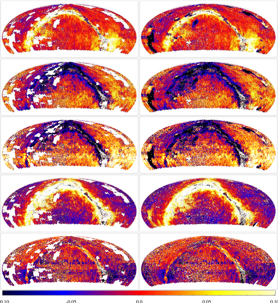
Figure 6.— Plots of the mean $J,H,K$ offsets and $J-H,H-K$ color offsets at fixed $g_{\rm P1}-i_{\rm P1}=0.5$. Left: Ubercal; Right: all PS1. The color scale shows the amplitude of the offset relative to the mean of the images. RA = 0.0 is at the center of the plots and increases to the left.

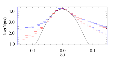
Figure 7.— Log histogram of $J$ offsets for all (blue lines; thick black line in print version) and Ubercal-only (red lines; thin black lines in the print version). Dotted lines show only the regions with $|b|>10.0$^∘. The black curve is a Gaussian fit to the peak of the high Galactic latitude Ubercal-only data ($\sigma=0.021$).

From inspection of per-exposure residuals, the cause of the higher scatter for non-photometric data is clear: with only a single zero point correction per exposure, we can only correct exposures to a limited extent. Those exposures with 2D variations in their effective extinction show up as trends in the residuals as a function of position, with corresponding higher scatter. In detailed examination, it is clear that a large fraction of these exposures with 2D attenuation patterns would be well-represented by a linear trend of the extinction with position. A future update to the photometric analysis will attempt to correct such image with a (minimal) 2D trend, after the full sky photometric coverage is improved.

The other important aspect of Figure 2 is the improved coverage resulting from the inclusion of exposures from non-photometric nights. The gaps in the Ubercal-only plots are filled in with the non-photometric nights. Note that in the Ubercal analysis, images from clearly non-photometric periods, as well as those from suspect periods, are rejected (either manually or automatically). This conservative cut allows for a very clean solution, but leaves us room to find an overlap solution that tiles across the gaps with confidence.

Table 3Pan-STARRS 1 Photometric Ladder Data Fields

FITS Name	CSV Seq	Description
RA	1	Right Ascension (degrees, J2000)
DEC	2	Declination (degrees, J2000)
X	$6\times N_{band}+3$	PSF-fit magnitude for PS1 band (X = $g_{\rm P1}$,$r_{\rm P1}$,$i_{\rm P1}$,$z_{\rm P1}$,$y_{\rm P1}$)
X:err	$6\times N_{band}+4$	formal error on magnitude
X:nphot	$6\times N_{band}+5$	number of measurements used for mean magnitude
X:stdev	$6\times N_{band}+6$	standard deviation of mean magnitude
X:flags	$6\times N_{band}+7$	flags for mean magnitude analysis
X:ucdist	$6\times N_{band}+8$	distance to Ubercal data in exposure footprints
J	8	2MASS J-band
H	9	2MASS H-band
K	10	2MASS K-band
X represents one of each filter $g_{\rm P1}$,$r_{\rm P1}$,$i_{\rm P1}$,$z_{\rm P1}$,$y_{\rm P1}$
$N_{band}$ is the filter sequence number $g_{\rm P1}$,$r_{\rm P1}$,$i_{\rm P1}$,$z_{\rm P1}$,$y_{\rm P1}$= (0,1,2,3,4)

For an additional check of the data quality, we employ a technique similar to the stellar locus analysis described by Ivezić et al. (2004) and Ivezić et al. (2007). Similar to that analysis, we have selected segments of the stellar locus in 3 2-color diagrams relevant to the PS1 data set: $g_{\rm P1}-r_{\rm P1},r_{\rm P1}-i_{\rm P1}$; $r_{\rm P1}-i_{\rm P1},i_{\rm P1}-z_{\rm P1}$; $i_{\rm P1}-z_{\rm P1},z_{\rm P1}-y_{\rm P1}$ (see Figure 3).

We define a reference stellar locus based on the stars in a 400 square-degree region of high Galactic latitude. We have selected only bright ($r_{\rm P1}<20.0$) objects with good measurements in all 5 filters and no evidence of extendedness. We have fitted a straight line segment to the portion of the locus for each 2-color diagram and determined principal colors ($P1,P2$) along and perpendicular to the locus in this region. The linear fits do not describe the stellar locus extremely well, so we have fitted a spline to the median in 0.05 magnitude wide bins along the $P1$ direction. We define $Q2$ as the corrected version of $P2$ with the spline fit subtracted. Similarly, there is a small trend of the $P2$ or $Q2$ color as a function of $r_{\rm P1}$, so we have again fitted a spline to the median in 0.25 magnitude wide bins in $r_{\rm P1}$. We define $S2$ as the corrected version of $Q2$ with this second spline fit subtracted. Note that the Ivezić et al. (2004) analysis used a linear fit for both color and magnitude corrections. The difference between the linear and spline fits is generally small ($<0.01$ mag), except for $i_{\rm P1}-z_{\rm P1},z_{\rm P1}-y_{\rm P1}$.

The intrinsic width of the stellar locus is quite small, and it is unclear if we have yet resolved it. In their analysis of the $g-r,r-i$ plane, Ivezić et al. (2004) determine an r.m.s. scatter in the $P2$ direction of 0.025 mags for single-epoch data, decreasing to 0.022 mags for 5-epoch data. Ivezić et al. (2007) show the $P2$ width decreasing to 0.010 mags in the many-epoch Stripe 82 data. Our plot of $P2$ vs $r_{\rm P1}$ (as well as $Q2$ and $S2$) shows a continued improvement to brighter objects, with an observed width of 0.012 magnitudes for $r_{\rm P1}<16.0$ (see Figure 3), quite comparable to the Stripe 82 observations from SDSS.

We have fitted the stellar locus defined above (for each 2-color plane) to the positions of stars for 0.5^∘boxes across the sky, using the same restrictions on magnitude range and quality when selecting the stars. In Figure 4, we present the mean offset of the observed stellar locus relative to the template for stars of $r_{\rm P1}<20.0$. In Figure 5, we present the scatter of the stellar locus for $r_{\rm P1}$ $<20.0$. Again this shows the high quality of the data using the ubercal analysis, but the limited coverage compared to the full $3\pi$ Survey area. These figures also illustrate that our relative photometric analysis can extend the regions of good coverage, but that the quality is sometimes degraded excessively.

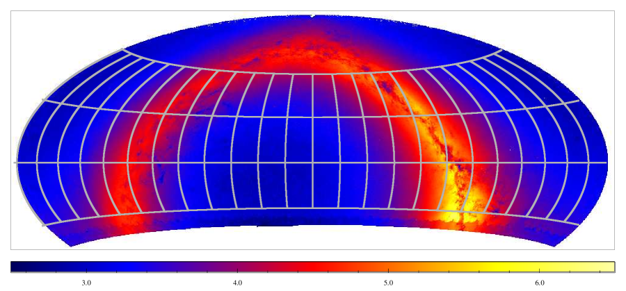
Figure 8.— Location of the photometric ladder overlayed on a plot of the spatial density of objects. The color scale gives the logarithm of the number of objects per square degree with at least 3 measurements and $r_{\rm P1}<19.0$. RA = 0.0 is at the center of the plots and increases to the left.

2.1.7 Comparisons with 2MASS

To explore how well relative photometry allows us to patch across the empty areas, we have compared our data to 2MASS observations, the only photometric dataset approaching our data quality and coverage (SDSS has large gaps in the regions of interest). For each 0.5^∘ pixel, we select the objects with high quality photometry ($g_{\rm P1}$, $r_{\rm P1}$, $i_{\rm P1}$ errors $<0.02$, standard deviations $<0.05$ magnitudes), excluding objects thought to be extended in these bands (based on PSF vs aperture photometry). We also exclude saturated objects. We then generate a color-color diagram in $g_{\rm P1}-r_{\rm P1},r_{\rm P1}-i_{\rm P1}$ and select the objects in the color range $0.2<g_{\rm P1}-r_{\rm P1}<1.0$, and within 0.05 magnitudes of the stellar locus in $g_{\rm P1}-i_{\rm P1}$. The resulting sample should be dominated by early type stars for which the optical / IR color-color loci are well defined.

We fit the color-color locus for the selected stars in each of the optical / IR color-color diagrams: $g_{\rm P1}-i_{\rm P1},i_{\rm P1}-J$; $g_{\rm P1}-i_{\rm P1},i_{\rm P1}-H$; $g_{\rm P1}-i_{\rm P1},i_{\rm P1}-K$. Finally, we determine ‘color offsets’, the fitted values of $i_{\rm P1}-J,H,K$ at a fixed $g_{\rm P1}-i_{\rm P1}$ value of 0.5. These color offsets are determined for each of the 0.5^∘ patches across the sky. If the data consisted of only stars with well-measured magnitudes and low extinction, the color offsets should be quite consistent across the sky. Extinction will shift the color-color loci, as well any photometric errors in either PS1 or 2MASS. At a lower level, changes in the mean metallicity or surface gravity of the relevant population can affect the color offsets as well. In Figure 6, we present maps of the color-offsets across the full $3\pi$ region. The left panels show only the Ubercal-tied data ($g_{\rm P1}$, $r_{\rm P1}$, $i_{\rm P1}$ all required), while the right panels show all data. The first three panels show the color offsets for $J,H,K$ respectively, while the last two panels show $J-H$ and $H-K$.

Several features can be seen in these plots. First, the Galactic Plane is clearly visible in all filters and combinations. This reflects the extinction sensitivity of these measurements. Further investigation of the 2D (and 3D) extinction patterns is ongoing and will be a major data product of the Pan-STARRS 1 $3\pi$ Survey (Schlafly et al., in prep).

Next, large scale structures can be seen which generally correspond to areas without Ubercal calibrations. This illustrates the difficulty of using relative photometry alone to tile across very large patches. While there are regions with acceptable consistency which lack Ubercal data, it is clear that the best quality photometry will only be possible when photometric data are available for essentially the whole survey region. Figure 7 shows the impact of Ubercal on the photometric residuals. In this figure, the blue line is a (log) histogram of the $i_{\rm P1}-J$ offsets using all data, while the red line shows the same using only the Ubercal measurements. The black line is a Gaussian fit to the core of the distribution, with $\sigma=0.023$ magnitudes. The positive outliers in this histogram come principally from the Galactic Plane, while the low end outliers show the impact of calibration errors on the non-Ubercal analysis.

Finally, there are visible patterns unrelated to any of the Pan-STARRS 1 observing pattern or sky tessellation. The strongest of these is the banding pattern seen in $K$ and $H-K$ running from RA $\sim 290$ to $\sim 90$, with boundaries at declinations of roughly 0.0, 6.0, 12.0, and 18.0^∘. At a lower level, a stripping pattern of narrow North-South bands a few RA degrees wide can also be seen. We believe these can be attributed to calibration offsets in the 2MASS data, especially in $K$ band. The amplitude of these patterns is consistent with a standard deviation of 2 - 3% for these regions.

This analysis, and comparisons between PS1 and SDSS (Finkbeiner et al., in prep) illustrate the difficulty of producing a single consistent photometric data product on a large scale. Especially for 2MASS and SDSS, the calibration is made additionally challenging by virtue of having only a single epoch for most of the survey area. The lack of internal repeat checks make it very difficult to prove that the calibrations are accurate across the whole survey region.

Even with multiple epochs, PS1 photometry calibration still has room for improvement, as can be seen in the figures above. However, as the PS1 survey is on-going, our expectation is that we will be able to fill in the non-photometric gaps in the upcoming years. The full power of the large-area and all sky surveys can be realized by combining the dataset to constrain and correct the systematics from all of these surveys.

3. DATA PRODUCTS

Table 4Bit-flags used to characterize average photometry values

FLAG NAME	Hex Value	Description
ID_SECF_USE_SYNTH	0x00000004	synthetic photometry used in average measurement
ID_SECF_USE_UBERCAL	0x00000008	Ubercal photometry used for average measurement
ID_PHOTOM_PASS_0	0x00000100	pass 0 : only use measurements thought to be GOOD (based on photometry analysis)
ID_PHOTOM_PASS_1	0x00000200	pass 1 : accept measurements thought to be POOR (based on photometry analysis)
ID_PHOTOM_PASS_2	0x00000400	pass 2 : accept the measurements marked as outliers based on relative photometry
ID_PHOTOM_PASS_3	0x00000800	pass 3 : accept measurements thought to be BAD (based on photometry analysis)
ID_PHOTOM_PASS_4	0x00001000	pass 4 : accept the measurements outside of the instrumental magnitude limits (eg, SAT)
ID_SECF_OBJ_EXT	0x01000000	possibly extended in this band

Over the next 1.5 - 2 years, Pan-STARRS 1 will finish the initial basic survey, completing coverage of the full $3\pi$ region. One of our major eventual goals is the production of a high-quality astrometric and photometric reference catalogs which can be used by observers to calibrate data with in-field references. The full survey dataset is necessary to pin down all regions at the highest possible precision. The vagaries of weather means that some substantial patches have not yet been observed in photometric conditions, and are only currently tied via relative photometry to the rest of the survey.

In this initial public release, we are providing the PS1 Reference Photometry Ladder as a sample of future Pan-STARRS 1 photometric calibration data. The Ladder consists of 4 strips in right ascension, 1 degree high, at declinations of (-25, 0, +25, +50), and 24 strips in declination, 1 RA degree wide centered on RA hours (see Figure 8).

We have selected a subset of bright ($g_{\rm P1},r_{\rm P1},i_{\rm P1}<19.14,19.26,19.24$), well-measured ($>4$ observations total) objects in these regions. The brightness limit was chosen to be equivalent to an instrumental magnitude of -9.5, or roughly 2% statistical errors. This brightness cut not only restricts the sample to objects with high signal-to-noise, it also avoids the stars affected by inconsistencies for faint stars. The inconsistencies we have observed take the form of variations in the measured flux for faint stars, relative to bright stars in the same images, as a function of seeing. We have also limited the density to $\sim 1000$ objects for each 1 square degree patch. To choose a high-quality sample at this limited density, we used the mean $\chi^{2}$ value for the $g_{\rm P1}$, $r_{\rm P1}$, and $i_{\rm P1}$ mean magnitudes to select the high-quality measurements. We then selected the 1000 objects for a given patch in ascending order of $\chi^{2}$ so that objects with consistent photometry are preferred.

The data are available from the PS1 Public Data web site.

We provide two sets of photometry tables: “Ubercal” and “Relphot”. The ubercal tables only include objects for which all 5 filters have measurements calibrated directly in the ubercal analysis. The relphot tables accept objects for which some filters have been tied to the ubercal data via relative photometry. As discussed above, the relphot values have lower confidence and should not be used for precision photometry. However, the relphot tables provide additional sky coverage. In most of these areas, a subset of the filters have ubercal photometry. Careful use of the per-filter flags is advised!

The tables are provided as FITS and comma-separated value tables. Table 3 defines the columns available in the tables. There are 27 separate tables, 1 for each of the ladder rungs in Dec and 1 for each of the rungs in RA. Note that there are duplicate entries between files where the rungs overlap.

Table 3 describes the fields provided for each object. Data for each of the five filters ($g_{\rm P1}$,$r_{\rm P1}$,$i_{\rm P1}$,$z_{\rm P1}$,$y_{\rm P1}$) are given in blocks, with 6 parameters provided for each filter. The magnitude provided is the mean PSF magnitude calibrated as described above. The error is the formal error determined by accepting the reported error from the photometric analysis for each separate measurement. $X:nphot$ represents the number of measurements actually used to determine the mean magnitude. Because of outlier clipping, this number may be smaller than the number of separate epochs available for a given object. The standard deviation of the mean magnitude is reported after clipping has been applied. The mean magnitude calculated for each filter is coupled to a set of bit-flags which describe the averaging process (Table 4). This value is reported as a 32-bit integer, but only the following 8 bits are used for each filter (see the discussion in Section 2.1.5).

To assess the extendedness of an object, we use the difference between the PSF and aperture magnitudes. If this difference is larger than 0.1 added in quadrature to 2.5 times the statistical error, then the measurement is considered extended. This measurement shows the presence of additional light in the aperture beyond the core consistent with the PSF model. The flag noting a possible extended object is raised if more than 50% of the measurements in a given band are observed to be extended based on this test.

Facilities: PS1 (GPC1)

References

- Anderson, G.P., et al. (2001) Anderson, G. P., et al. 2001, Proc. SPIE 4381, 455
- Bessel (1990) Bessel, M. S. 1990, PASP 102, 1181
- Chambers et al. (in prep) Chambers, K. C., et al., in preparation.
- Finkbeiner et al. (in prep) Finkbeiner, D. P., et al., in preparation.
- Hodapp et al. (2004) Hodapp, K. W., Siegmund, W. A., Kaiser, N., Chambers, K. C., Laux, U., Morgan, J., & Mannery, E. 2004, Proc. SPIE 5489, 667
- Hsieh et al. (2012) Hsieh, H. H., Yang, B., Haghighipour, N., Kaluna, H. M., Fitzsimmons, A., et al., 2012, Asteroids, Comets, Meteors 2012, Proceedings of the conference held May 16-20, 2012 in Niigata, Japan. LPI Contribution No. 1667, id.6313.
- Ivezić et al. (2004) Ivezić, Z., Lupton, R. H., Schlegel D., et al., 2004, Astronomische Nachrichten 325, 583.
- Ivezić et al. (2007) Ivezić, Z., Smith, A., Miknaitis G., et al., 2007, AJ 134, 973
- Johnson et al. (2009) Johnson, J. A., Winn, J. N., Cabrera, N. E., Carter, J. A. (2009) ApJ 692, L100
- Kaiser et al. (2010) Kaiser, N., et al. 2010, Proc. SPIE 7733, 12K.
- Magnier (2006) Magnier, E. 2006, Proceedings of The Advanced Maui Optical and Space Surveillance Technologies Conference, Ed.: S. Ryan, The Maui Economic Development Board, p.E5
- Narayan et al. (2011) Narayan, G., Foley, R. J., Berger, E., et al. 2011, ApJ 731, L11
- Onaka et al. (2008) Onaka, P., Tonry, J. L., Isani, S., Lee, A., Uyeshiro, R., Rae, C., Robertson, L., & Ching, G. 2008, Proc. SPIE 7014, 12O
- Padmanabhan et al. (2008) Padmanabhan, N., Schlegel, D. J., Finkbeiner, D. P., et al. 2008, ApJ 674, 1217
- Tonry & Onaka (2009) Tonry, J., & Onaka, P. 2009, Advanced Maui Optical and Space Surveillance Technologies Conference, Proceedings of the Advanced Maui Optical and Space Surveillance Technologies Conference, Ed.: S. Ryan, p.E40.
- Tonry et al. (2005) Tonry, J. L., Howell, S. B., Everett, M. E., Rodney, S.A., Willman, M., VanOutryve, C. 2005, PASP 117, 218
- Tonry et al. (2012) Tonry, J. L., Stubbs, C. W., Lykke, K. R., Doherty, P., Shivvers, I. S., Burgett, W. S., Chambers, K. C., Hodapp, K. W., Kaiser, N., Kudritzki, R.-P., Magnier, E. A., Morgan, J. S., Price, P. A., Wainscoat, R. J. 2012, ApJ 750, 99
- Schlafly et al. (2012) Schlafly, E. F., Finkbeiner, D. P., Jurić, M., Magnier, E. A., Burgett, W. S., Chambers, K. C., Grav, T., Hodapp, K. W., Kaiser, N., Kudritzki, R.-P., Martin, N. F., Morgan J. S., Price, P. A., Stubbs, C. W., Tonry, J. L., Wainscoat, R. J. 2012, ApJ 756, 158.
- Schlafly et al. (in prep) Schlafly, E. F., et al. 2012, in preparation
- York et al. (2000) York, D. G., Adelman, J., Anderson Jr., J. E., Anderson, S. F., Annis, J., Bahcall, N. A., Bakken, J. A., Barkhouser, R., Bastian, S., Berman, E., Boroski, W. N., Bracker, S., et al., 2000, AJ 120, 1579.