Three-dimensional Keplerian orbit-superposition models of the nucleus of M31

Abstract

We present three-dimensional eccentric disc models of the nucleus of M31, modelling the disc as a linear combination of thick rings of massless stars orbiting in the potential of a central black hole. Our models are nonparametric generalisations of the parametric models of Peiris & Tremaine. The models reproduce well the observed WFPC2 photometry, the detailed line-of-sight velocity distributions from STIS observations along P1 and P2, together with the qualitative features of the OASIS kinematic maps.

We confirm Peiris & Tremaine’s finding that nuclear discs aligned with the larger disc of M31 are strongly ruled out. Our optimal model is inclined at $57^{\circ}$ with respect to the line of sight of M31 and has position angle P.A.$=\theta_{l}+90^{\circ}=55^{\circ}$. It has a central black hole of mass $M_{\bullet}\simeq 1.0\times 10^{8}\,M_{\odot}$, and, when viewed in three dimensions, shows a clear enhancement in the density of stars around the black hole. The distribution of orbit eccentricities in our models is similar to Peiris & Tremaine’s model, but we find significantly different inclination distributions, which might provide valuable clues to the origin of the disc.

1 Introduction

As the nearest spiral galaxy to our own, M31 allows the study of a galactic centre in unmatched detail. A particularly striking feature of high-resolution $V$- and $I$-band photometry of the central few arcseconds of M31 is its double nucleus (Light et al., 1974; Lauer et al., 1993; Bacon et al., 1994; King et al., 1995): there are two peaks in surface brightness, the brighter of which (known as P1) is extended and offset $\sim 0\aas@@fstack{\prime\prime}5$ from the fainter peak (known as P2), which is elongated and close to the photometric centre of the bulge. Early spectroscopic observations resolved steep gradients in the stellar rotation velocities and a prominent peak in the stellar velocity dispersion, which hints at the presence of a massive black hole (Dressler & Richstone, 1988; Kormendy, 1988; Bacon et al., 1994; van der Marel et al., 1994).

Tremaine (1995) put forward an elegant explanation for these observations: the nucleus is a massive disc of red stars on eccentric, nearly Keplerian, approximately aligned orbits around a central black hole located at P2; P1 is generated by orbital crowding of stars lingering at apocentre. Subsequent observations have been consistent with his model. Lauer et al. (1998) observed the nucleus with the Wide Field Planetary Camera 2 (WFPC2) on the corrected Hubble Space Telescope (HST), confirming the bimodal structure. Kormendy & Bender (1999) obtained spectroscopy with the Subarcsecond Imaging Spectrograph (SIS) finding an asymmetric rotation curve and a constant colour across the nucleus, showing P1 and P2’s colours to be consistent with each other but not the bulge or a globular cluster. Further kinematics were recorded with the Faint Object Camera (Statler et al., 1999), the integral field spectrograph OASIS (Bacon et al., 2001) and the Space Telescope Spectroscopy Imaging Spectrograph (STIS) on HST (Bender et al., 2005). All of these observations show that the kinematic centre of the nucleus is very close to P2, as predicted by T95’s eccentric disc model.

Further refinement of this picture has come from studying the nucleus at ultraviolet wavelengths. Almost all of the UV emission from the nucleus comes from a tiny ($<0\aas@@fstack{\prime\prime}1$) source located at P2 (King et al., 1995; Lauer et al., 1998; Brown et al., 1998), whose optical–UV colours and spectra are consistent with a population of A stars (Lauer et al., 1998; Bender et al., 2005), distinct from the red K-type spectrum of the rest of the nucleus (Bender et al., 2005). Bender et al. (2005) find that this compact, young, blue population has a maximum velocity dispersion of $\sigma=1183\pm 201$ km s^-1, significantly higher than the red stars’ $\approx 250$ km s^-1. They label the UV peak P3 and have found that its photometry and kinematics are well modelled by a separate, almost-circular disc of blue stars around a central black hole of mass ($1.1$-$2.3)\times 10^{8}M_{\odot}$. This provides very strong evidence in support of the presence of a supermassive black hole, which is the most fundamental requirement of T95’s model. Most recently, Lauer et al. (2012) has found that the surface brightness profile of the young population is described by an exponential profile of scale length $0\aas@@fstack{\prime\prime}075\pm 0\aas@@fstack{\prime\prime}01$.

Tremaine’s original eccentric disc model consisted of three Keplerian orbits, coplanar with the main disc of M31, projected onto the sky and convolved with Gaussian point spread functions (PSFs). The original model included neither disc self-gravity nor a realistic treatment of the disc’s internal velocity dispersions but was still able to broadly reproduce kinematic features. To be stable over many dynamical times such a disc would require apsidal alignment to be maintained; T95 proposed that this could be achieved by the disc self-gravity and argued that two-body relaxation would lead to a disc thickness of $\approx 0.3$ times the disc radius. Estimates of the disc mass from mass to light ratios place it at around $10^{7}M_{\odot}$. This is substantial enough to affect the dynamics of the disc although the nucleus falls within the sphere of influence of the black hole, which dominates the orbits and imposes regularity. A self-gravitating eccentric disc mode maintaining orbital alignment would also precess under a uniform pattern speed. Since the T95 model, several two-dimensional self-gravitating models with these properties have been constructed (Statler, 1999; Bacon et al., 2001; Salow & Statler, 2001; Sambhus & Sridhar, 2002; Salow & Statler, 2004). These massive models have found a variety of disc masses, pattern speeds and orbital distributions.

Peiris & Tremaine (2003) took a different approach. They revised the 1995 model and constructed fully three-dimensional models with a parametric distribution function that ignored the self gravity of the disc; the gravitational potential in their models is due solely to the central black hole, which greatly simplifies the modelling procedure. Their models are the most successful to date at fitting the observed kinematics. They also found that thickened disc models that were misaligned with respect to the large-scale M31 disc produced significantly better fits than coplanar models, echoing a result seen in the 2d models.

The current picture of the nucleus (see figure 1) has the black hole (hereafter BH) embedded in P3, which is explained by a flat, circular exponential disc of blue stars 0$\aas@@fstack{\prime\prime}$033 from the photometric bulge centre. This young, blue disc is surrounded by the larger, red, eccentric disc. P1 is made of stars crowding at apoapsis, while P2 is now identified as stars at pericenter in the elongated region on the anti-P1 side of P3. The system remains of great interest: the origin of the nuclei and the relationship between the red and blue populations are unexplained and the mass and pattern speed of precession of the disc have not been pinned down consistently. Understanding the dynamics of the disc will help determine the BH mass more accurately which is of use in better determining the relationship between a BH and the host galaxy. It is also of interest to confirm whether the eccentric disc is aligned with the main disc of M31.

In this paper we present a natural development of the modelling approach started by Peiris & Tremaine (2003). Like them, we ignore the self-gravity of the disc, leaving the construction of fully self-gravitating models for a subsequent paper. But instead of considering parameterised functional forms for the phase-space distribution function (hereafter DF) of the nucleus, we model the DF non-parametrically as a mixture of Gaussian rings whose amplitudes are allowed to vary: one of our goals is to “let the data speak for themselves” and then examine closely the structure of the DF. The paper is organised as follows. In section 2 we summarise the data we use and additional post-processing applied. Section 3 describes our modelling procedure and section 4 our results. Section 5 sums up.

Throughout this paper we adopt a distance of 770kpc to M31.

2 Observational Data

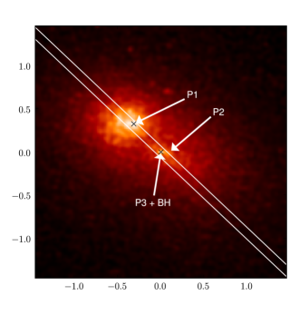
Figure 1: $V$-band image of the nucleus (Lauer et al., 1998) annotated to show the relative positions of P1, P2 and P3 in arcseconds. The pair of white lines represents the positioning and width of the STIS slit (Bender et al., 2005). The brightest point in the image is at P1 and is marked with cross. Centred in the image and marked with a cross is the location of the black hole and P3. P2 is on the anti-P1 side of the black hole.

Our models use observations from three instruments: the HST photometry recorded with WFPC2, detailed in Lauer et al 1998 (hereafter L98), the high resolution kinematics from STIS (Bender et al 2005, B05) and the kinematic maps from the integral field spectrograph OASIS (Bacon et al 2001, hereafter B01).

2.1 Photometry

We use the deconvolved $V$-band (F555W) WFPC2 photometry of L98. This image is 1024$\times$1024 pixels in size with a pixel scale of 0$\aas@@fstack{\prime\prime}$011375. P3 is located at (513, 518). We note that the orientation of the image has North 82.3^∘ clockwise from the y-axis - the data has been rotated away from the original alignment of the CCD, so that the corners of the image are blank - but we make no attempt to reorient the image. This image has already been reduced and deconvolved but we perform some processing on the image in order to reduce this data to a tractable number of observables for our fitting procedure. Bright foreground stars are first masked out and we crop the image to a 512$\times$512 pixel region centred on P3. This is a region of side 5$\aas@@fstack{\prime\prime}$824 and incorporates the nucleus and the inner parts of the bulge and removes the blank corners of the image. This cropped image is then rebinned to "super-pixels" of side $2^{l}$ pixels containing the mean of the $2^{2l}-n$ pixels, with $n$ the number of masked pixels falling in the super-pixel. We consider two schemes for choosing super-pixels: in the first we simply take $l=2$ everywhere so that super-pixels contain a $4\times 4$ pixel region. In the other $l$ is chosen based on the surface brightness of the image scaled by $r^{-1/2}$, where $r$ is the radius from P3, to provide a good balance of detail around P2 and P1. This gives $l=0$ (the resolution of the deconvolved image) at P1 and P2 and $l=4$ in the outermost parts of the image. A total of 4096 super-pixels are generated in this scheme.

Ajhar et al (1997) and Lauer et al (1998) showed that that at the resolution of WFPC2 the underlying number of stars in M31 shows strong surface brightness fluctuations. The limited number of stars is the dominant residual between the structure of the nucleus and any model we fit. We treat the noise from the fluctuations as the sole source of our errors in our photometry and ignore photon noise so that the fractional error in a spatial bin is given by $\sigma=\bar{N}^{-1/2}$, where $\bar{N}$ is the effective number of stars within the spatial bin. L98 gives the effective magnitude of each SBF “star” as $\bar{m}_{I}=23.4$, or $224\,L_{\odot}$. The error associated with a spatial bin containing $n\,L_{\odot}$ is therefore $\sqrt{224n}\,L_{\odot}$.

2.2 STIS kinematics

The STIS kinematics are taken from Table 5 of Bender et al. (2005). These consist of the bulge-subtracted Gauss–Hermite coefficients derived with the Fourier Correlation Quotient Method at the 22 positions listed for each of $V$, $\sigma$, $h_{3}$ and $h_{4}$ and their accompanying errors. We adopt the same slit widths of 0.1″and position angle of 39^∘. The quoted positions are given with respect to the location of P3.

We use equation (21) of Peiris & Tremaine (2003) to model the STIS PSF. When this is convolved with a a $0\aas@@fstack{\prime\prime}1$-square top hat to represent the slit, the result is well approximated by a double Gaussian

$$\mathop{\hbox{PSF}}(x,y)=\frac{1}{\sum_{i}I_{i}}\sum_{i=1}^{2}\frac{I_{i}}{2\pi\sigma_{i}^{2}}e^{-\frac{(x^{2}+y^{2})}{2\sigma_{i}^{2}}}$$ (1)

with amplitudes $I_{1}=0.24$, $I_{2}=0.76$ and dispersions $\sigma_{1}=0\aas@@fstack{\prime\prime}042$ and $\sigma_{2}=0\aas@@fstack{\prime\prime}087$ respectively. We assume that equation (1) as the effective PSF of the STIS observations. A more sophisticated treatment might take account of asymmetries in the PSF and the variations in spatial binning along the slit.

2.3 OASIS kinematics

We also make use of the kinematics of the integral field spectrograph OASIS, which were kindly provided by Eric Emsellem. We opt to use the higher S/N data set, M8. This consists of $V$, $\sigma$, $h_{3}$ and $h_{4}$ values derived from spectra taken at 1123 positions, spaced by 0$\aas@@fstack{\prime\prime}$09. We registered the image with the WFPC2 data using a similar process to B01. We found a close match in angle (0.7^∘) and a small offset of (-0$\aas@@fstack{\prime\prime}$02, -0$\aas@@fstack{\prime\prime}$03) between the two images.

Like B01 we assumed that the OASIS measurements have a PSF that can be described by a sum of three Gaussians and allowed the parameters of these Gaussians to float freely in the registration process, taking the form

$$\mathop{\hbox{PSF}}(x,y)=\frac{1}{\sum_{i}I_{i}}\sum_{i=1}^{3}\frac{I_{i}}{2\pi\sigma_{i}^{2}}e^{-\frac{(x^{2}+y^{2})}{2\sigma_{i}^{2}}}$$ (2)

The resulting PSF differs from that found by B01 with $\sigma_{1}=0\aas@@fstack{\prime\prime}230$, $\sigma_{2}=0\aas@@fstack{\prime\prime}587$, $\sigma_{3}=0\aas@@fstack{\prime\prime}440$ and $I_{2}/I_{1}=0.836$ and $I_{3}/I_{1}=0.057$.

3 Modelling procedure

Our models are straightforward generalisations of those of PT. In particular, we ignore the self gravity of the disc and the gravitational influence of the bulge and assume that the potential is purely Keplerian. The mass of the central black hole $M_{\bullet}$ is the single free parameter in our model potential. We assume that the BH is located at P3.

3.1 Coordinate systems

Following PT03 we use three different coordinate systems: “orbit plane”, “disc plane” and “sky plane”. All three coordinate systems have origin $O$ coincident with the BH. Our models have biaxial symmetry. This provides a natural definition of the “disc plane” $(x,y,z)$ coordinate system: the model is symmetric under reflections in the $(x,y)$ and $(x,z)$ planes. The orbit-plane and sky-plane coordinate systems are defined as follows. In the potential of the BH all orbits are Keplerian ellipses. An orbit with semi-major axis $a$ and eccentricity $e$ defines a coordinate system $(x^{\prime},y^{\prime},z^{\prime})$ in which the $Oz^{\prime}$ axis is parallel to the orbit’s angular momentum vector and the $Ox^{\prime}$ axis points towards pericentre. That is,

$$\begin{split}x^{\prime}=&\;a(\cos E-e),\\ y^{\prime}=&\;a\sqrt{1-e^{2}}\sin E,\\ z^{\prime}=&\;0,\end{split}$$ (3)

where the eccentric anomaly $E$ is related to the mean anomaly $M$ through Kepler’s equation $M=E-e\sin E$. In this coordinate system the apocentre of the orbit is located at $(x^{\prime},y^{\prime},z^{\prime})=(-a(1+e),0,0)$ and the pericentre at $(a(1-e),0,0)$. Each star defines its own orbit-plane $(x^{\prime},y^{\prime},z^{\prime})$ coordinate system.

A star’s disc-plane coordinates $(x,y,z)$ are related to its orbit-plane coordinates $(x^{\prime},y^{\prime},z^{\prime})$ through

$$\begin{split}\begin{pmatrix}x\\ y\\ z\end{pmatrix}&=\begin{pmatrix}\cos\Omega&-\sin\Omega&0\\ \sin\Omega&\cos\Omega&0\\ 0&0&1\end{pmatrix}\begin{pmatrix}1&0&0\\ 0&\cos I&-\sin I\\ 0&\sin I&\cos I\end{pmatrix}\\ &\qquad\times\begin{pmatrix}\cos\omega&-\sin\omega&0\\ \sin\omega&\cos\omega&0\\ 0&0&1\end{pmatrix}\begin{pmatrix}x^{\prime}\\ y^{\prime}\\ z^{\prime}\end{pmatrix},\end{split}$$ (4)

where the angles $\omega$, $I$ and $\Omega$ are the star’s argument of periapsis, the inclination and longitude of the ascending node, respectively. Any orbit in the Keplerian potential of the BH can be labelled by the five integrals of motion $(a,e,\omega,I,\Omega)$, but it proves convenient to replace $e$ and $\omega$ by the eccentricity vector ${\bf e}\equiv(e\cos\varpi,e\sin\varpi,0)=(e_{x},e_{y},0)$, where the longitude of periapsis $\varpi=\omega+\Omega$. The vector ${\bf e}$ points from the BH towards the projection of the pericentre onto the $z=0$ disc plane. Its magnitude is the scalar eccentricity $e$ of the orbit.

Projected, sky-plane coordinates $(X,Y,Z)$ are related to disc plane coordinates via

$$\begin{split}\begin{pmatrix}X\\ Y\\ Z\end{pmatrix}&=\begin{pmatrix}\cos\theta_{l}&-\sin\theta_{l}&0\\ \sin\theta_{l}&\cos\theta_{l}&0\\ 0&0&1\end{pmatrix}\begin{pmatrix}1&0&0\\ 0&\cos\theta_{i}&-\sin\theta_{i}\\ 0&\sin\theta_{i}&\cos\theta_{i}\end{pmatrix}\\ &\qquad\times\begin{pmatrix}\cos\theta_{a}&-\sin\theta_{a}&0\\ \sin\theta_{a}&\cos\theta_{a}&0\\ 0&0&1\end{pmatrix}\begin{pmatrix}x\\ y\\ z\end{pmatrix},\end{split}$$ (5)

in which $(\theta_{a},\theta_{i},\theta_{l})$ are the three Euler angles specifying the orientation of the disc with respect to the observer’s reference frame. The $(X,Y)$ plane is the sky plane, with the positive $X$ axis pointing west and positive $Y$ axis north. The $Z$ axis then points towards the observer; the line-of-sight velocity is therefore $V_{\rm los}=-\dot{Z}$, following the usual convention that that receding objects have $V_{\rm los}>0$.

3.2 Distribution function

We model only the old stellar population of the disc; the young stars around P3 and the bulge are treated as contaminants (see §3.4 below). Assuming that the old stars are collisionless and homogenous, their dynamics can be completely described by a distribution function (DF) $f({\bf x},{\bf v})$, defined such that $f({\bf x},{\bf v})\,{\rm d}^{3}{\bf x}\,{\rm d}^{3}{\bf v}$ is the expected number of such stars within a small phase-space volume ${\rm d}^{3}{\bf x}\,{\rm d}^{3}{\bf v}$ around the point $({\bf x},{\bf v})$. We further assume that the system is in a steady state. By Jeans’ theorem the DF must be expressible as a function of the integrals of motion $(a,{\bf e},I,\Omega)$. The number of stars within a small phase-space volume element ${\rm d}^{3}{\bf x}{\rm d}^{3}{\bf v}$ is then

$$f({\bf x},{\bf v}){\rm d}^{3}{\bf x}{\rm d}^{3}{\bf v}=f(a,{\bf e},I)\,\frac{1}{2}(GM_{\bullet})^{3/2}a^{1/2}\sin I{\rm d}I\,{\rm d}a{\rm d}{\bf e}{\rm d}\Omega{\rm d}M,$$ (6)

the $\frac{1}{2}(GM_{\bullet})^{3/2}a^{1/2}\sin I$ factor coming from the Jacobian relating $({\bf x},{\bf v})$ to $(a,{\bf e},I,\Omega,M)$.

We assume that the distribution function can be decomposed into a weighted sum of rings,

$$f=\sum_{j}{w_{j}f_{j}(a,{\bf e},I)},$$ (7)

in which each ring has a uniform distribution of $\Omega\in[0,2\pi)$ and Gaussian distributions in $a$, ${\bf e}$, $I$,

$$\begin{split}f_{j}(a,{\bf e},I)=&N_{j}\exp{\left[-\frac{(a-a_{j})^{2}}{2{\sigma_{a,j}}^{2}}\right]}\exp{\left[-\frac{({\bf e}-{\bf e}_{j})^{2}}{2{\sigma_{{\bf e},j}}^{2}}\right]}\times\\ &\exp{\left[-\frac{I^{2}}{2{\sigma_{I,j}}^{2}}\right]},\end{split}$$ (8)

and it is understood that $f_{j}(a,{\bf e},I)=0$ if $a<0$ or $|{\bf e}|>1$. The normalisation factor $N_{j}$ is included to give each ring unit total luminosity. We use a Monte Carlo method to construct the rings, which avoids explicit calculation of $N_{j}$.

Our rings span a $(20\times 9\times 4)$ grid in $(a_{j},e_{x,j},\sigma_{I,j})$, with mean semimajor axis $a_{j}$ running logarithmically from $0\aas@@fstack{\prime\prime}03$ to $10^{\prime\prime}$, mean $x$ component of eccentricity vector $e_{x,j}$ from $-0.8$ to $+0.8$ in steps $\Delta e=0.2$, and the dispersion in inclination $\sigma_{I,j}$ drawn from $\{12^{\circ},24^{\circ},36^{\circ},48^{\circ}\}$. For the spreads in $(a,e)$ we take $\sigma_{a,j}=0.8a_{j}\Delta\log a$ and $\sigma_{e,j}=0.8\Delta e=0.16$. All rings have mean $e_{y,j}=0$. Together with the zero mean inclination of each ring this makes our models symmetric under reflection in the $y=0$ and $z=0$ planes. Rings with mean $e_{x}>0$ are “aligned” in the sense that their apocentre (and therefore peak density) lies somewhere along the negative $x$ axis. Rings with mean $e_{x}<0$ have the opposite orientation.

3.3 Observables of each ring

We compute the projected properties of each ring $f_{j}$ (equ. 8) by sampling it with $10^{6}$ points, drawing $N_{o}=5000$ values of $(a,{\bf e},I,\Omega,\omega)$ from the distribution $f_{j}(a,{\bf e},I)a^{1/2}\sin I$ that appears on the right-hand side of (6), then sampling 200 points equispaced in mean anomaly $M$ along each of these orbits. To avoid sampling artefacts we select the initial value of $M$ for each orbit at random.

3.3.1 WFPC

We use this sample of $10^{6}$ points to estimate the projected surface density (or, equivalently, the zeroth velocity moment)

$$\mu^{0,\rm fine}_{j}(X,Y)\equiv\int{\rm d}Z{\rm d}V_{X}{\rm d}V_{Y}{\rm d}V_{Z}\,f_{j}$$ (9)

on a fine grid of $0\aas@@fstack{\prime\prime}011375\times 0\aas@@fstack{\prime\prime}011375$ pixels on the $(X,Y)$ sky plane by simply counting the number of points that fall within each pixel. The contribution of the $j^{\rm th}$ ring to each WFPC2 “superpixel” is found by taking the mean value of $\mu^{0,\rm fine}_{j}(X,Y)$ over the relevant range of $(X,Y)$. We do not carry out any PSF convolution for the WFPC2 photometry because the image of Lauer et al. (1998) has already been deconvolved.

3.3.2 OASIS

The OASIS kinematics of Bacon et al. (2001) consist of measurements of mean velocity $V(X,Y)$ and velocity dispersion $\sigma(X,Y)$, together with Gauss-Hermite coefficients $h_{3}(X,Y)$ and $h_{4}(X,Y)$. We ignore their $h_{3}$ and $h_{4}$ measurements and assume that their measured $V(X,Y)$ and $(V^{2}+\sigma^{2})(X,Y)$ distributions probe directly the (PSF-convolved) first- and second-order moments of the line-of-sight velocity distribution (LOSVD) at the point $(X,Y)$ on the sky. This is a good approximation provided the underlying PSF-convolved LOSVDs are reasonably close to Gaussian. For modelling purposes it is more natural to consider luminosity-weighted moments

$$\begin{split}\mu^{1}(X,Y)&\equiv I(X,Y)V(X,Y),\\ \mu^{2}(X,Y)&\equiv I(X,Y)(V^{2}+\sigma^{2})(X,Y),\end{split}$$ (10)

where $I(X,Y)$ is the underlying surface brightness. We obtain $I(X,Y)$ by convolving the WFPC2 image with the OASIS PSF (2). The observational errors on these first- and second-order luminosity-weighted velocity moments are obtained by adding the uncertainties on $I$, $V$ and $\sigma$ in quadrature in the obvious way:

$$\begin{split}(\Delta\mu^{1})^{2}&=(\Delta I)^{2}V^{2}+I^{2}(\Delta V)^{2}\\ (\Delta\mu^{2})^{2}&=(\Delta I)^{2}(V^{2}+\sigma^{2})+I^{2}(2|V|\Delta V)^{2}+I^{2}(2\sigma\Delta\sigma)^{2}.\end{split}$$ (11)

Following (9) above, the contribution of the $j^{\rm th}$ ring to the luminosity-weighted first and second moments of the line-of-sight velocity distribution,

$$\begin{split}\mu^{1,\rm fine}_{j}(X,Y)&\equiv\int{\rm d}Z{\rm d}V_{X}{\rm d}V_{Y}{\rm d}V_{Z}\,V_{Z}f_{j},\\ \mu^{2,\rm fine}_{j}(X,Y)&\equiv\int{\rm d}Z{\rm d}V_{X}{\rm d}V_{Y}{\rm d}V_{Z}\,V_{Z}^{2}f_{j},\end{split}$$ (12)

are estimated by weighting each of the $10^{6}$ sample points by $V_{Z}$ and $V_{Z}^{2}$, respectively. Having these $\mu^{i,\rm fine}_{j}(X,Y)$ distributions we convolve with the OASIS PSF (2) to obtain the contribution the ring makes to the model’s predictions for the first and second velocity moments of the OASIS kinematics.

3.3.3 STIS

Our first attempt at fitting the STIS kinematics was based on the same assumption that we could use the STIS $V$ and $\sigma$ measured by B+05 as direct estimates of the (STIS PSF-convolved) first- and second-order moments of the LOSVD. That did not work well: at STIS resolution the LOSVDs are far from Gaussian, as we show on Figure 2, and the strong high-velocity wings caused by the BH mean that it is not possible to obtain reliable estimates of the first and second moments from the observed spectra. This last point was one of the motivations for the introduction of Gauss–Hermite series (van der Marel & Franx, 1993) to parametrize LOSVDs. Therefore we fit our models to B+05’s Gauss–Hermite parametrizations of the LOSVDs along the STIS slit. Our method for fitting the Gauss–Hermite coefficients follows the same lines used in other orbit-superposition models (e.g., Cretton et al. (1999)), but taking extra care to treat the normalisation of the LOSVDs correctly.

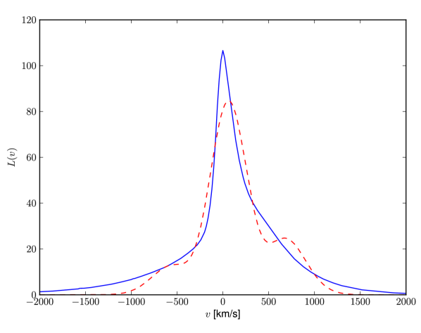
Figure 2: LOSVD of a typical model at offset $R=0\aas@@fstack{\prime\prime}2$ along the STIS slit (solid blue curve) and its 4-th order Gauss–Hermite reconstruction (equ 16, dashed red curve). The best-fit Gaussian to the LOSVD has $(\gamma,V,\sigma)=(0.81,-85{\,\rm km\,s^{-1}},281{\,\rm km\,s^{-1}})$. For comparison, the classical zeroth-, first- and second-order moments of this LOSVD are 1, $V_{0}=-36\,\rm km\,s^{-1}$ and $\sigma_{0}=759\,\rm km\,s^{-1}$, the latter being dominated by the strong high-velocity wings.

We recall some details of Gauss–Hermite expansions. Suppose that we are given an LOSVD $L_{0}(v)$, normalised such that $\int L_{0}(v)\,{\rm d}v=1$. The Gauss–Hermite expansion of this $L_{0}(v)$ is

$$L(v|\gamma,V,\sigma)=\frac{\gamma\alpha(w)}{\sigma}\sum_{j=0}^{\infty}h_{j}H_{j}(w),$$ (13)

where $w\equiv(v-V)/\sigma$, $\alpha(w)={\rm e}^{-w^{2}/2}/\sqrt{2\pi}$ is the standard Gaussian and the $H_{j}(w)$ are Hermite polynomials. We adopt vdMF93’s normalisation for the latter. Using the orthogonality properties of the $H_{j}$, it is easy to show that the Gauss–Hermite coefficients $h_{l}$ are given by

$$h_{l}(\gamma,V,\sigma)=\frac{2\sqrt{\pi}}{\gamma}\int_{-\infty}^{\infty}L_{0}(v)H_{l}(w)\alpha(w){\rm d}v.$$ (14)

That is, there is a different Gauss–Hermite series (13) for each choice of $(\gamma,V,\sigma)$. The “line-strength” parameter $\gamma$ simply scales all the $h_{j}$, but it proves important as we shall now see.

A particularly natural choice of the parameters $(\gamma,V,\sigma)$ are those that minimise

$$\chi_{0}^{2}=\int_{-\infty}^{\infty}\left[L_{0}(v)-\frac{\gamma\alpha(w)}{\sigma}\right]^{2}\,{\rm d}v,$$ (15)

in which case it can be shown that the first few Gauss–Hermite coefficients from (14) become $h_{0}=1$ and $h_{1}=h_{2}=0$. In other words, if we choose $(\gamma,V,\sigma)$ to be the parameters of the best-fit Gaussian to the LOSVD $L(v)$, then the LOSVD can be written as

$$L(v)=\frac{\gamma\alpha(w)}{\sigma}\left[1+\sum_{j=3}^{\infty}h_{j}H_{j}(w)\right],$$ (16)

with $h_{3}$, $h_{4}$, … given by the integral (14). Conversely, if we adopt the parametrization (16) and fit $(\gamma,V,\sigma,h_{3},h_{4},...)$ simultaneously to $L_{0}(v)$, then we get back the same parameters we would obtain by first fitting $(\gamma,V,\sigma)$ by minimising (15) and then using (14) to find the $h_{i}$. For a strongly non-Gaussian $L_{0}(v)$ the parameters $(\gamma,V,\sigma)$ obtained by minimising (15) need not be close to zeroth-, first- and second-order moments of $L_{0}(v)$, as shown on Figure 2. In particular, $\gamma$ need not be close to 1.

Gauss–Hermite fits to the LOSVDs of real galaxies, including B+05’s measurements of M31, adopt the parametrization (16) and fit $(\gamma,V,\sigma,h_{3},h_{4},...)$. Unfortunately, the parameter $\gamma$ is rarely reported, presumably because it is strongly affected by systematic effects in the fitting procedure, such as template mismatch, and because it does not affect the shape or width of the LOSVDs. Nevertheless, we note that it is an essential part of any Gauss–Hermite expansion. For now we assume that $\gamma$ is known. Our iterative scheme for reconstructing it from the models is described in section 4.3 below.

Notice that equation (14) shows that the Gauss–Hermite coefficients $h_{l}$ can be thought of as modified moments: each $h_{l}$ is the integral over velocity space of some linear combination of the classical moments $1,w,w^{2},...,w^{l}$, but weighted by the Gaussian factor $\alpha(w)$. Therefore, given a Gauss–Hermite fit $(\gamma,V,\sigma,h_{3},h_{4})$ to the line-of-sight velocity distribution at projected position $(X,Y)$, we treat $(\gamma,V,\sigma)$ as being known perfectly and take the (luminosity-weighted) modified moments $(\tilde{\mu}^{0}_{\rm obs},...,\tilde{\mu}^{4}_{\rm obs})\equiv I\times(1,0,0,h_{3},h_{4})$ as our observables, where the surface brightness $I(X,Y)$ is obtained by convolving the WFPC2 image by the STIS PSF (1). We use equations (10) of vdMF93 to propagate B+05’s quoted uncertainties $(\Delta V_{i},\Delta\sigma_{i},\Delta h_{3,i},\Delta h_{4,i})$ to our observational errors $(\Delta\tilde{\mu}^{0}_{i,\rm obs},...,\Delta\tilde{\mu}^{4}_{i,\rm obs})$.

Just as for the classical velocity moments, for each ring $j=1,2,...$ we use our Monte Carlo sample of $10^{6}$ positions and velocities to evaluate the expressions

$$\begin{split}\tilde{\mu}_{j}^{k,\rm fine}(X,Y|{\gamma},V_{i},\sigma_{i})&\equiv\frac{\sqrt{2}}{\gamma_{i}}\int{\rm d}Z{\rm d}V_{X}{\rm d}V_{Y}{\rm d}V_{Z}\\ &\quad\times\exp\left[-\frac{1}{2}w^{2}\right]H_{k}(w)\,f_{j}\end{split}$$ (17)

for the modified moments, in which the rescaled velocity

$$w\equiv\frac{(-V_{Z})-V_{i}}{\sigma_{i}}.$$ (18)

Then we convolve each of these distributions with the STIS PSF (1) and read off the values at $(X,Y)=(X_{i},Y_{i})$, giving the contribution of the $j^{\rm th}$ ring to the $k^{\rm th}$ modified moment of the $i^{\rm th}$ STIS data point, $\tilde{\mu}^{k}_{i,\rm obs}$.

3.4 Modelling the effects of the bulge and P3

Our ring system is designed to model only the old red stars of the eccentric disc, but some of the light observed in the central few arcsec of M31 comes from other sources. The two main contaminants are M31’s bulge and the compact young stellar cluster at P3.

We follow Kormendy & Bender (1999) in modelling the surface brightness of the bulge as a Sersic profile $I(R)=I_{0}\exp(-(R/R_{n})^{1/n})$ with index $n=2.19$, scale radius $R_{n}=14\aas@@fstack{\prime\prime}0$ and central $V$-band surface brightness $I_{0}=15.40$ mag. Our kinematic model for the bulge is very simple: it is non rotating and has a constant velocity dispersion $\sigma_{\rm bulge}=120{\,\rm km\,s^{-1}}$. We add the contribution from this simple bulge model to our models’ predictions for the WFPC2 photometry and the OASIS $V$ and $\sigma$ maps. We do not add it to the STIS predictions; we assume that B05 have successfully removed the bulge contribution from their STIS kinematics.

To model the contribution the young stars from P3 make to the $V$-band light we include a another component having surface brightness $\Sigma(X,Y)=\Sigma_{3}\exp(-R/R_{0})$ in which $R^{2}=X^{2}+Y^{2}$ and the scale length $R_{0}=0\aas@@fstack{\prime\prime}075$ (L12). We follow B05 in assuming that the kinematics extracted from the red spectra are unaffected by the young stars; these stars affect only the WFPC2 photometry, not the OASIS or STIS kinematics.

3.5 Fitting the weights

For given BH mass $M_{\bullet}$ and disc orientation $(\theta_{a},\theta_{i},\theta_{l})$, the model’s prediction for any observable $O_{i}$ can be be written as $\sum_{j}P_{ij}w_{j}$, in which $w_{j}$ is the weight given to the $j^{\rm th}$ ring (equ. 7) and the matrix $P_{ij}$ gives the contribution that the $j^{\rm th}$ ring makes to the $i^{\rm th}$ observable, calculated using the method described in §3.3 above. An observable $O_{i}$ can be the light within a “superpixel” (given by WFPC2 photometry), a classical first- or second-order velocity moment (OASIS kinematics) or a $0^{\rm th}$…$4^{\rm th}$-order modified moment (STIS kinematics). We do not include the zeroth-order moments of the OASIS kinematics as these contain no additional information over the WFPC2 photometry.

Having a vector of observables $(O_{1},O_{2},....)$ and associated uncertainties $(\Delta_{1},\Delta_{2},\ldots)$, we use a non-negative linear least squares algorithm (Lawson & Hanson, 1974) to find the vector of non-negative weights ${\bf w}$ that minimises

$$\chi^{2}=\sum_{i}\left[\frac{O_{i}-\sum_{j}P_{ij}w_{j}}{\Delta_{i}}\right]^{2}.$$ (19)

We then take this minimum value of $\chi^{2}$ as a measure of the goodness of fit of the model with parameters $(M_{\bullet},\theta_{l},\theta_{i},\theta_{a})$.

4 Results

Ideally, we would like to include all data sets (WFPC2, STIS, OASIS) in our set of $O_{i}$ and fit simultaneously to them. However, calculating the contribution the $j^{\rm th}$ ring makes to a particular modified moment is computationally intensive and a full study of the parameter space spanned by $M_{\bullet}$, $\theta_{l}$, $\theta_{i}$ and $\theta_{a}$ that includes the STIS and OASIS data sets is not viable. We therefore conduct our modelling in two stages. We first fit models to the WFPC2 photometry and the OASIS velocity distribution in order to find the best set of orientation angles $(\theta_{a},\theta_{i},\theta_{l})$. Then, having these angles, we fit to the WFPC2 photometry and STIS kinematics to obtain our estimates of the BH mass and the structure of the phase-space DF of the nucleus. As a final test of this model, we “observe” it at OASIS resolution and compare it (by eye) to the real M31.

Before embarking on any of this model fitting, however, we first confirm that our models are indeed able to reproduce some of PT03’s results.

4.1 A test: reproducing PT03’s model

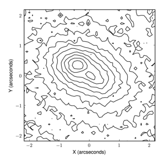
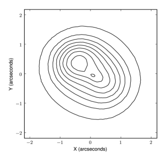
Figure 3: Nuclear V-band surface brightness distribution. The left panel shows the data and the right our reconstruction of Peiris & Tremaine’s (2003) non-aligned model. Contours are at 0.25 mag intervals. Compare to figure 3 of PT03.

An immediate test of our modelling machinery is to reproduce some of PT03’s results by using a sum of rings (8) that approximates one of their DFs. We focus here on their favoured non-aligned model, but we found comparable results with the poorer-fitting model that is forced to be aligned with the main M31 disc. PT03’s non-aligned models have DF

$$f(a,{\bf e},I)=g(a)\exp\left\{-\frac{[{\bf e}-{\bf e}_{m}(a)]^{2}}{2\sigma_{e}^{2}}\right\}\exp\left[-\frac{I^{2}}{2\sigma_{I}(a)^{2}}\right],$$ (20)

where $\sigma_{e}=0.307$. The parametric form for the backbone eccentricities is given by

$${\bf e}_{m}(a)=\alpha(a_{e}-a)\exp\left[-\frac{(a-a_{g})^{2}}{2w^{2}}\right]\hat{\bf x},$$ (21)

with $\alpha=0.197\,\rm pc^{-1}$, $a_{e}=4.45$ pc, $a_{g}=1.71$ pc and $w=1.52$ pc. For the dispersion in inclination the form is

$$\sigma_{I}(a)=\sigma_{I}^{0}\exp(-a/a_{I})$$ (22)

where $\sigma_{I}^{0}=24\aas@@fstack{\circ}6$ and $a_{I}=31.5$ pc. The function $g(a)$ that sets the semi-major axis distribution is

$$g(a)=\Sigma_{0}\frac{a^{2}\exp(-a/a_{0})}{1+\exp[c_{1}(a-c_{2})]}\;\frac{a^{1/2}}{2\pi^{2}(GM_{\bullet})^{3/2}\sigma_{e}^{2}\sigma_{I}^{2}(a)},$$ (23)

with $a_{0}=1.37$ pc, $M_{\bullet}=10.2\times 10^{8}M_{\odot}$, $c_{1}=4$ pc^-1 and $c_{2}=4.24$ pc. We treat the overall normalisation $\Sigma_{0}$ as a free parameter.

We approximate this DF by a sum of 720 rings of the form (8) whose semi-major axes $a_{j}$ are spaced logarithmically in radius from 0.1 pc to 19 pc, with $\sigma_{a,j}=0.8a_{j}\Delta\log a$. We set $\sigma_{e,j}=0.307$ for all rings and set the mean eccentricity ${\bf e}_{j}$ and dispersion in inclination $\sigma_{I,j}$ of the $j^{\rm th}$ ring by evaluating (21) and (22) above at $a=a_{j}$. The weights $w_{j}$ are set proportional to $a_{j}g(a_{j})$, the factor of $a_{j}$ coming from the fact that our rings are equispaced in $\log a$.

Figure 3 shows the resulting model predictions for the WFPC2 photometry when viewed at the same angles as PT03’s best-fit non-aligned model ($\theta_{a}=-34\aas@@fstack{\circ}5$, $\theta_{i}=54\aas@@fstack{\circ}1$, $\theta_{l}=-42.8\aas@@fstack{\circ}2$) and including the contribution of the bulge model from sec. 3.4. Our reconstruction of the projected surface brightness in their model agrees closely with their figure 3: the model produces a nucleus that is broader than the observations and has an overly extended flat profile at P1.

4.2 Determining the orientation of the disc

We conduct an exhaustive scan over the space of orientation angles $(\theta_{a},\theta_{i},\theta_{l})$ and black hole mass to obtain our best guess for the orientation of the disc. We first do this for a model that is forced to be aligned ($\theta_{i}=77\aas@@fstack{\circ}5$) with the larger-scale M31 disc, before letting $\theta_{i}$ vary freely. We include in these fits the 1123 OASIS $V$ data points as well as a broad field spanning $5\aas@@fstack{\prime\prime}824\times 5\aas@@fstack{\prime\prime}824$ from the WFPC2 data: this utilises our varied super-pixel scheme and contains 4096 data points. We do not include the OASIS $\sigma$ maps in the fits, as it is dangerous to assume that the measured $V^{2}+\sigma^{2}$ is a good estimate of the true second moment of the LOSVD (figure 2).

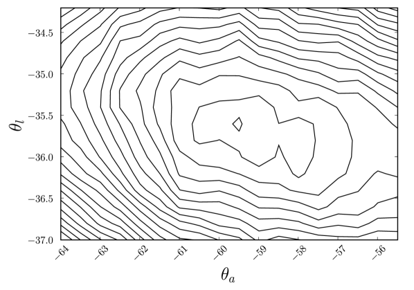
Figure 4: $\chi^{2}$ for $\theta_{l}$ vs. $\theta_{a}$ for the aligned model. Contours are spaced at $\Delta\chi^{2}=4$ intervals.

For the aligned model we fix $\theta_{i}=77\aas@@fstack{\circ}5$ and take $\theta_{a}$ and $\theta_{l}$ in the intervals [$-90^{\circ}$, $0^{\circ}$] and [$-55^{\circ}$, $-25^{\circ}$] with spacing $\Delta\theta=2^{\circ}$. A contour plot depicting the shape of the $\chi^{2}$ goodness of fit for the inner region of this range is shown in figure 4. As expected the aligned model constrains $\theta_{l}$ tightly but there is a weak dependence on $\theta_{a}$, with the best fitting model falling at $\theta_{a}=-60^{\circ}$ and $\theta_{l}=-35^{\circ}$.

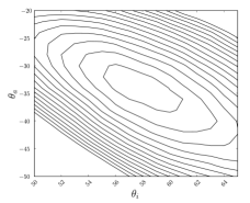
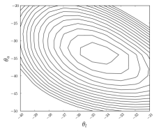
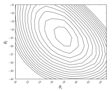
Figure 5: Contour maps of $\chi^{2}$ for the slice through the best fitting model. From left to right: $\theta_{i}$ vs. $\theta_{a}$ for $\theta_{l}=-35^{\circ}$; $\theta_{l}$ vs. $\theta_{a}$ for $\theta_{i}=57^{\circ}$; $\theta_{i}$ vs. $\theta_{l}$ for $\theta_{a}=-34^{\circ}$. Contours are spaced by $\Delta\chi^{2}=25$.

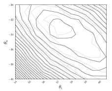
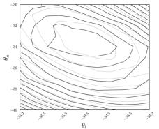
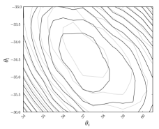
Figure 6: Zoomed in contour maps. From left to right: $\theta_{i}$ vs. $\theta_{a}$; $\theta_{l}$ vs. $\theta_{a}$; $\theta_{i}$ vs. $\theta_{l}$. Contours are spaced by $\Delta\chi^{2}=7.5$. The black contours show the same distribution as figure 5. The grey contours show an alternative realisation of the distribution function to illustrate the effect of shot noise.

The non-aligned model looks at $\theta_{a}$ from $-58^{\circ}$ to $-20^{\circ}$, $\theta_{i}$ from $50^{\circ}$ to $69^{\circ}$ and $\theta_{l}$ from $-39^{\circ}$ to $-29^{\circ}$, with $\Delta\theta_{a}=2^{\circ}$ and $\Delta\theta_{l}=\Delta\theta_{i}=1^{\circ}$. The best fit appears at $\theta_{a}=-34^{\circ}$, $\theta_{i}=57^{\circ}$, $\theta_{l}=-35^{\circ}$ for a black hole mass $M_{\bullet}\simeq 1.25\times 10^{8}M_{\odot}$. The shape of the $\chi^{2}$ goodness of fit for the non-aligned model is shown in figure  5. The presented scan is for a single random distribution of stars projected with different angles: scans using distributions drawn from a different random seed found broadly similar results with slight variations (figure 6). This presents issues with determining a single best fitting set of angles. Using a much larger ($10^{8}$) number of stars per disc in the region around the best fit angles informed our final selection of specific angles, however even then the random seed affected results. While in principle the angles could be determined more accurately, in practice shot noise from the model (and also the finite number of stars in the real nucleus!) limits the accuracy in each angle to the order of $\approx 1^{\circ}$. Our final selection of angles was determined from the projection of the likelihood $\exp(-\frac{1}{2}\chi^{2})$ onto each of the $\theta_{a}$, $\theta_{i}$ and $\theta_{l}$ axes.

We have experimented with allowing the bulge surface brightness $I_{0}$ and the central surface brightness $\Sigma_{3}$ of the young stellar disc described in sec. 3.4 to float our fitting procedure by including them as additional “weights” $w_{j}$ in the model and adding two additional columns to the projection matrix $P_{ij}$, but we find that this makes little difference to our results.

4.3 Fitting WFPC2 photometry and STIS kinematics

Having the orientation angles we now drop the OASIS $V$ maps and focus on using WFPC2 photometry together with the STIS LOSVDs to further constrain the model. The region of the WFPC2 photometry we use is restricted to an ellipse of semi-major axis $1\aas@@fstack{\prime\prime}6$ and axis ratio 0.6 centred on P2. This ellipse is just large enough to encompass all STIS positions. We rebin Lauer et al. (1998)’s dithered image 4 by 4 into “superpixels” of side 0$\aas@@fstack{\prime\prime}$0455. Our vector of observables $O_{i}$ consists of the WFPC2 fluxes in all 2335 such superpixels that lie within the ellipse, together with the 5 modified moments $(\tilde{h}_{i,0},...,\tilde{h}_{i,4})$ obtained from $(\gamma_{i},V_{i},\sigma_{i},h_{3,i},h_{4_{i}})$ for each of the $i=1...22$ LOSVDs measured by Bender et al. (2005) using the procedure described earlier in section 3.3.3.

4.3.1 Reconstruction of the $\gamma(R)$ profile

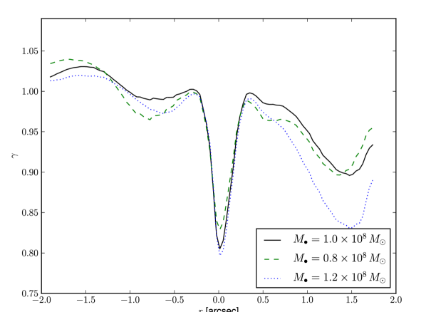
Figure 7: The Gauss–Hermite “line-strength” parameter $\gamma$ reconstructed along the STIS slit using the iterative procedure described in section 4.3 for three different assumed black hole masses, as indicated on the legend.

The only complication in this is that we do not know the line strengths $\gamma$ for any of our LOSVDs. We do, however, expect $\gamma$ to be reasonably close to one and so we first fit a model in which all $\gamma_{i}=1$. Then, having the weights $w_{j}$, we construct a realization of this model and “observe” it convolved with the STIS PSF (1). We fit Gauss–Hermite coefficients $(\gamma,V,\sigma,h_{3},h_{4})$ to the model LOSVDs at each point along the STIS slit, giving us a more informed estimate of how $\gamma$ varies along the slit. We then repeat the whole fitting procedure, replacing our original $\gamma_{i}=1$ guesses with values read off from this reconstructed $\gamma(R)$ distribution. We find that the resulting model converges after only a couple of iterations of this scheme. Figure 7 plots representative $\gamma$ profiles obtained by this procedure for models with black hole masses $M_{\bullet}/10^{8}M_{\odot}=1.0$, 0.8 and 1.2. This shows that $\gamma$ is significantly depressed close to the black hole where the LOSVDs are least well described by simple Gaussians.

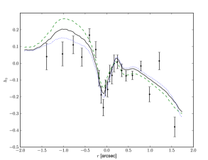
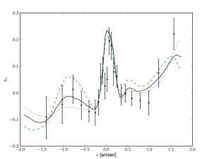
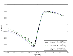
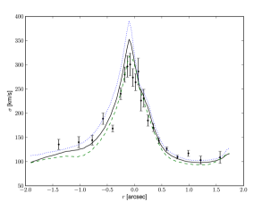
Figure 8: Gauss–Hermite coefficients parametrising the LOSVDs along the STIS slit measured by B05 (points) together with our model fits for three different assumed black hole masses (curves).

4.3.2 Comparison of best-fit model against observations

The formal $\chi^{2}$ of the model with $M_{\bullet}=1.0\times 10^{8}M_{\odot}$ is 782. To put this in perspective, the vector of observables $O_{i}$ that the model fits has 2445 elements: 2335 WFPC2 fluxes plus $5\times 22$ modified moments. For comparison, the model with $M_{\bullet}=0.8\times 10^{8}\,M_{\odot}$ has $\chi^{2}=825$, while the model with $M_{\bullet}=1.2\times 10^{8}\,M_{\odot}$ has $\chi^{2}=859$. Figure 8 shows the Gauss–Hermite coefficients of the reconstructed models along the STIS slit. The agreement with B05’s observed kinematics is good, but there some features the best $M_{\bullet}=1.0\times 10^{8}\,M_{\odot}$ model cannot reproduce: the model does not fit the detailed shape of the $V(R)$ and $h_{3}(R)$ profiles between $R=-0\aas@@fstack{\prime\prime}9$ and $0\aas@@fstack{\prime\prime}3$ well and it predicts a central $\sigma(R)$ that is slightly too high.

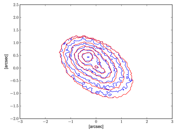
Figure 9: Observed $V$-band WFPC2 image (blue) with the fit from our $M_{\bullet}=1.0\times 10^{8}M_{\odot}$ overlaid on top (red). Contours are spaced at 0.3 magnitude intervals.

Figure 9 shows how well the $M_{\bullet}=1.0\times 10^{8}\,M_{\odot}$ model fits to the WFPC2 photometry. Results for the other two black hole masses are similar. The agreement is good in the central regions, but beyond about 1 arcsec from P2 the model’s surface brightness profile falls off too slowly compared to the observations. One possible explanation for this is that our model is simply too coarse; the thickness of each of the $n_{a}=20$ rings (equ. 8) in these models is $\sigma_{a}=0.23a$, which sets the models’ characteristic radial spatial resolution. Another is that our model for the contribution of the bulge light (sec. 3.4) may be wrong within the innermost couple of arcsec.

Based on these comparisons, we interpret the relatively low values of $\chi^{2}$ of our models not as a indication of the outstanding quality of our model fits, but instead as a sign that the treatment of the observational uncertainties – particularly of the WFPC2 photometry – could be improved. Nevertheless, we believe that the reader will agree that simple “chi-by-eye” tests indicate that our models produce the best fits to date of the M31 eccentric disc system. Of course, this is to be expected given that we have $>700$ free parameters to play with, which is at least an order of magnitude more than most previous models of M31’s nucleus.

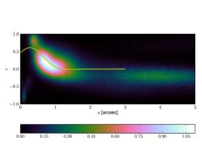
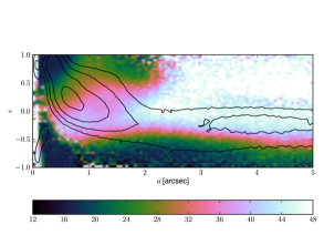
Figure 10: The distribution of orbits in our best-fit model with $M_{\bullet}=1.0\times 10^{8}\,M_{\odot}$. Left panel: the projected DF $f(a,e_{x})$ obtained from the full DF $f(a,e_{x},e_{y},I)$ by averaging over $e_{y}$ and $I$. The yellow curve plots the $a(e_{x})$ profile of PT03’s best-fit model for comparison. Right panel: RMS inclination angle (in degrees) as a function of $(a,e_{x})$ obtained from $f(a,e_{x},e_{y},I)$ by averaging over $e_{y}$. The $f(a,e_{x})$ distribution from the left panel is overlaid as contours.

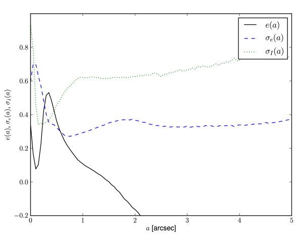
Figure 11: Mean eccentricity $e_{x}(a)$ and dispersions in eccentricity $\sigma_{e,x}(a)$ and inclination $\sigma_{I}(a)$ as a function of semi-major axis $a$. Unlike figure 10 the dispersion $\sigma_{I}$ in this plot is given in radians, not degrees.

4.3.3 DF of best-fitting model

What can we learn from all these free parameters, specifically the orbit weights $w_{j}$? Figure 10 shows two views of the DF $f(a,e_{x},e_{y},I)$ of our best-fit model. This model has a strong negative eccentricity gradient between 0$\aas@@fstack{\prime\prime}$5 and 1$\aas@@fstack{\prime\prime}$2 (corresponding to P1), which is very similar to PT03’s best-fit model; even the dispersion in eccentricity (figure 11) is similar to their value of $0.307$. There are three important differences between our model and theirs, however.

1. Beyond 1$\aas@@fstack{\prime\prime}$2 the mean eccentricity in our models becomes negative, meaning that the rings become mildly antialigned. We find that the strength of this feature depends on the details of our bulge model and so it is hard to judge its significance, but we note that just such a feature was predicted by Statler (1999) in his analysis of thin, self-gravitating discs.

2. Whereas PT03’s parametrised model had an exponentially declining $\sigma_{I}$ profile, our model fits a $\sigma_{I}$ profile that increases with radius for $a>0\aas@@fstack{\prime\prime}15$. This last point is qualitatively consistent with the predictions of collisional models of disc evolution (Stewart & Ida, 2000; Peiris & Tremaine, 2003). The detailed agreement is not so good though: whereas the collisional models predict $\sigma_{I}/\sigma_{e}\simeq 0.5$, our models fit $\sigma_{I}/\sigma_{e}\simeq 2$. It is not immediately clear, however, how far one can apply these calculations that assume almost circular $e=0$ discs to the strongly eccentric disc in M31.

3. $f(a)$ in our model falls steeply towards the centre from $a=0\aas@@fstack{\prime\prime}5$ to $a\simeq 0\aas@@fstack{\prime\prime}15$, inside which there is antialigned ($e_{x}\simeq-0.5$), fat ($\sigma_{I}=48^{\circ}$) distribution of orbits. Recall that the range of $\sigma_{I}$ reproducible by our chosen sample of rings is from $12^{\circ}$ to $48^{\circ}$. This distinctive change in the distribution of the red stars is almost cospatial with the young, A-star population that make up P3.

4.3.4 Other projections of the best-fit model

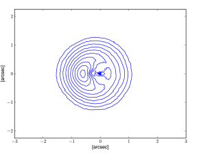
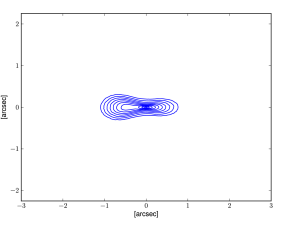
Figure 12: Face-on ($xy$, left) and edge-on ($xz$, right) projected surface brightness distributions of our best-fit model. Contours are spaced at 0.2 magnitudes.

Figure 12 shows the face-on and edge-on projected density distributions of our best-fit model. Our machinery fits a density distribution which, when viewed face on, is broadly similar to the density distribution adopted by Salow & Statler (2004) in their self-gravitating razor-thin models. Apart from our neglect of self gravity, the most significant difference between our models and theirs is that ours have a secondary density peak around P2 and also have significant thickness.

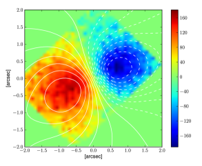
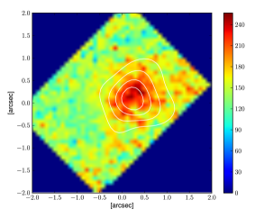
Figure 13: OASIS $V$ (left) and $\sigma$ (right) maps predicted by our models (white contours) compared to the observations from B01. The contours in both panels are spaced $25\,\rm km\,s^{-1}$ apart. The $V$ contours run from 0 to $\pm 175\,\rm km\,s^{-1}$, $\sigma$ from 150 to $225\,\rm km\,s^{-1}$.

Although the models we present in this section are not fit to the OASIS maps, we can nevertheless compare our reconstructed models’ predictions against the real OASIS maps. Figure 13 shows the results for the $M_{\bullet}=1.0\times 10^{8}\,M_{\odot}$ model. The model reproduces the shape and orientation of velocity and dispersion maps very well. This provides an independent test of the orientation angles and the broad-brush features of the DF inferred by our models.

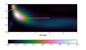
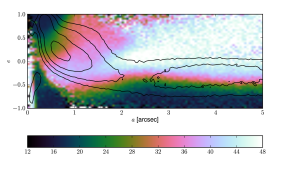
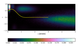
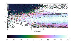
Figure 14: The distribution of orbits in a model that includes both prograde and retrograde orbits. The top two panels show the DF $f(a,e_{x})$ (left) and the rms inclination (right) for the prograde stars. The bottom two panels show the corresponding distributions for the retrograde population.

4.3.5 A brief experiment: retrograde orbits

Finally, we note that one proposed origin of the eccentric disc in M31 is from an $m=1$ instability in an initially circular stellar disc that contains a small counter-rotating population of stars (Touma, 2002; Jog & Combes, 2009; Kazandjian & Touma, 2012). $N$-body simulations of this instability (Kazandjian & Touma, 2012) show that the dominant, prograde population becomes the eccentric disc, while the minor, retrograde population is puffed up into a strongly triaxial distribution. As a quick experiment to test whether this is easily detectable, we have tried doubling up our ring distribution by including in our models the retrograde ring corresponding to each of the 720 prograde rings considered above, giving a total of 1440 rings. This produces a noticeably better fit to the observations, with $\chi^{2}=784$ instead of 812, with the fitting procedure picking out three main counter-rotating components (figure 14) at $(a,e)=(0\aas@@fstack{\prime\prime}2,0.8)$, $(1\aas@@fstack{\prime\prime}2,0.6)$ and $(3,-0.1)$. None of these is easily identifiable with the more diffuse component predicted by Kazandjian & Touma (2012), although we suspect that that might be hard to detect with naive models such as ours. We interpret the innermost retrograde ring as suggesting that our ring-based decomposition fails at radii $r<0\aas@@fstack{\prime\prime}2$, perhaps by not being fine enough. Similarly, we take the presence of the other two rings as a hint that our bulge model could perhaps be improved.

5 Conclusions

We have constructed an eccentric disc models of the nucleus of M31 by modelling it as a linear combination of fattened rings of stars orbiting in a purely Keplerian potential. Our models are an obvious generalisation of those of PT03 and – as expected – are noticeably (albeit perhaps not significantly) more successful at reproducing the features observed in the inner arcsec or so of M31.

One of the most fundamental parameters of any model of this system is its orientation. Like PT03, we assume that the disc has biaxial symmetry, but we find some differences in the Euler angles $(\theta_{a},\theta_{i},\theta_{l})$ that specify the orientation of these symmetry axes. Our values of $\theta_{a}=-34^{\circ}$ and $\theta_{i}=57^{\circ}$ agree reasonably well with their $\theta_{a}=-34\aas@@fstack{\circ}5$ and $\theta_{i}=54\aas@@fstack{\circ}51$, but our value of $\theta_{l}=-35^{\circ}$ (which directly controls the position angle on the sky) differs significantly from their $\theta_{l}=-42\aas@@fstack{\circ}8$, more than can be accounted for by the effects of shot noise in either the models or in the distribution of stars in the real disc.

Our orientation is also consistent with the N-body model of B01 ($\theta_{i}=55^{\circ}\pm 5^{\circ}$ and $\theta_{l}=-36^{\circ}$) and the models of Salow & Statler (2004) ($\theta_{i}=63\aas@@fstack{\circ}51\pm 10\aas@@fstack{\circ}80$ and assumed $\theta_{l}=-33\aas@@fstack{\circ}6$) and Sambhus & Sridhar (2002) ($\theta_{i}=51\aas@@fstack{\circ}54$ and $\theta_{l}=27\aas@@fstack{\circ}34$), though it should be noted all these models are 2d which imposes constraints on their geometry; Sambhus & Sridhar (2002) obtained their orientation by de-projecting the photometry of the disc such that the outer isophotes became circular. We note that these values of $\theta_{i}$ found for the old, red distribution of stars are close to the inclination of the young population in P3 ($\theta_{i}=55^{\circ}\pm 2^{\circ}$) measured by B+05.

The most interesting result of our models is the DF they infer from the data, bearing in mind that they contain no prior “wisdom” about which DFs are dynamically plausible. The models suggest the presence of a distinct, compact disc of red stars within 0$\aas@@fstack{\prime\prime}$15 of the black hole. This disc is anti-aligned (with eccentricity $e<0$) with respect to the larger-scale eccentric disc (which has $e>0$). Outside this compact region the eccentricity distribution of our models is very similar to PT03’s. The main difference between our models and theirs is in the inclination distribution: our models fit an RMS inclination profile $\sigma_{I}(a)$ that closely tracks the dispersion in eccentricity, with $\sigma_{I}(a)/\sigma_{e}(a)\simeq 2$. This is interesting: models of the collisional evolution of (circular) discs predict that this ratio should be $\sim 0.5$.

Another difference between our models and PT03 is that we find evidence for an anti-aligned feature $(e<0)$ at $a>1\aas@@fstack{\prime\prime}5$. However, the details of this feature depend on our assumed bulge model, which merits further investigation.

Our models prefer black hole masses $M_{\bullet}$ of the order of $1.0\times 10^{8}\,M_{\odot}$; masses higher than about $1.2\times 10^{8}\,M_{\odot}$ are weakly ruled out. Although it would be possible to use our machinery to carry out a full scan of black hole masses and orientation angles, followed by a systematic investigation of the degeneracies in the DF, we believe that a more pressing task is to include the self gravity of the disc. The stars contribute a significant fraction ($\sim 20\%$) of the mass of the BH+eccentric disc system, which means that it is dangerous to read too much into our present, purely Keplerian models. Past 2d (Bacon et al., 2001; Sambhus & Sridhar, 2002; Salow & Statler, 2004, e.g.,) models have shown it is possible to get plausibly good fits to the kinematics for large disc masses. The space of 3d disc distributions that project to yield the observed surface brightness profile is degenerate, but our orbital ring system serves as a good starting point for this investigation. Work on self-gravitating self-consistent 3d disc models is now underway, and we hope that such models will provide further insight into the origin of the eccentric disc in M31 and possibly elsewhere (Lauer et al., 2005).

References

- Ajhar et al. (1997) Ajhar, E. A., Lauer, T. R., Tonry, J. L., Blakeslee, J. P., Dressler, A., Holtzman, J. A., Postman, M. 1997, AJ, 114, 626
- Bacon et al. (1994) Bacon, R., Emsellem, E., Monnet, G., & Nieto, J. L. 1994, A&A, 281, 691
- Bacon et al. (2001) Bacon, R.; Emsellem, E.; Combes, F.; Copin, Y.; Monnet, G.; Martin, P. 2001, A&A, 371, 409
- Bender et al. (2005) Bender, R., Kormendy, J., Bower, G., et al. 2005, ApJ, 631, 280
- Brown et al. (1998) Brown, T. M., Ferguson, H. C., Stanford, S. A., & Deharveng, J.-M. 1998, ApJ, 504, 113
- Cretton et al. (1999) Cretton, N., de Zeeuw, P. T., van der Marel, R. P., & Rix, H.-W. 1999, ApJS, 124, 383
- Dressler & Richstone (1988) Dressler, A., & Richstone, D. O. 1988, ApJ, 324, 701
- Jog & Combes (2009) Jog, C. J., & Combes, F. 2009, Phys. Rep., 471, 75
- Kazandjian & Touma (2012) Kazandjian, M. V., & Touma, J. R. 2012, arXiv:1207.1108
- King et al. (1995) King, I. R., Stanford, S. A., & Crane, P. 1995, AJ, 109, 164
- Kormendy (1988) Kormendy, J. 1988, ApJ, 325, 128
- Kormendy & Bender (1999) Kormendy, J., & Bender, R. 1999, ApJ, 522, 772
- Lauer et al. (1993) Lauer, T. R., Faber, S. M., Groth, E. J., et al. 1993, ApJ, 106, 1436
- Lauer et al. (1998) Lauer, T. R., Faber, S. M., Ajhar, E. A., Grillmair, C. J., & Scowen, P. A. 1998, ApJ, 116, 2263
- Lauer et al. (2005) Lauer, T. R., et al., 2005, AJ129 2138
- Lauer et al. (2012) Lauer, T. R., Bender, R., Kormendy, J., Rosenfield, P., & Green, R. F. 2012, ApJ, 745, 121
- Lawson & Hanson (1974) Lawson, C. L., & Hanson, R. J. 1974, Prentice-Hall Series in Automatic Computation, Englewood Cliffs: Prentice-Hall, 1974,
- Light et al. (1974) Light, E. S., Danielson, R. E., & Schwarzschild, M. 1974, ApJ, 194, 257
- Peiris & Tremaine (2003) Peiris, H. V., & Tremaine, S. 2003, ApJ, 599, 237
- Salow & Statler (2001) Salow, R. M., & Statler, T. S. 2001, ApJ, 551, L49
- Salow & Statler (2004) Salow, R. M., & Statler, T. S. 2004, ApJ, 611, 245
- Sambhus & Sridhar (2002) Sambhus, N., & Sridhar, S. 2002, A&A, 388, 766
- Statler (1999) Statler, T. S. 1999, ApJ, 524, L87
- Statler et al. (1999) Statler, T. S., King, I. R., Crane, P., & Jedrzejewski, R. I. 1999, AJ, 117, 894
- Stewart & Ida (2000) Stewart G. R., Ida S., 2000, Icarus, 143, 28
- Touma (2002) Touma, J. R. 2002, MNRAS, 333, 583
- Tremaine (1995) Tremaine, S. 1995, ApJ, 110, 628
- van der Marel & Franx (1993) van der Marel, R. P., & Franx, M. 1993, ApJ, 407, 525
- van der Marel et al. (1994) van der Marel, R. P.; Rix, H. W.; Carter, D.; Franx, M.; White, S. D. M.; de Zeeuw, T. 1994, MNRAS, 268, 521