Low-Complexity Adaptive Set-Membership Reduced-rank LCMV Beamforming

Abstract

This paper proposes a new adaptive algorithm for the implementation of the linearly constrained minimum variance (LCMV) beamformer. The proposed algorithm utilizes the set-membership filtering (SMF) framework and the reduced-rank joint iterative optimization (JIO) scheme. We develop a stochastic gradient (SG) based algorithm for the beamformer design. An effective time-varying bound is employed in the proposed method to adjust the step sizes, avoid the misadjustment and the risk of overbounding or underbounding. Simulations are performed to show the improved performance of the proposed algorithm in comparison with existing full-rank and reduced-rank methods.

I Introduction

Adaptive beamforming technology has received considerable attention for several decades and found widespread applications in radar, sonar and wireless communications [2]. The optimal linearly constrained minimum variance (LCMV) beamformer [3] which minimizes the array output power while maintaining the array response on the direction of the desired signal, is the most well-known beamformer. However, the computation of the inverse of the received data covariance matrix and the requirement of the knowledge of the cross-correlation vector present difficulties for its implementation.

A number of adaptive algorithms have been reported for the implementation of the LCMV beamformer [2], [4]. Among them the stochastic gradient (SG) algorithm [5], [6] is popular due to its simplicity and low complexity. The drawback of the SG algorithm is that the convergence depends on the eigenvalue spread of the received data covariance matrix. This condition could be worse when the number of elements in the filter is large since it requires a large amount of snapshots to reach the steady-state.

Reduced-rank signal processing was introduced to provide a way out of this dilemma [8]-[15]. The reduced-rank schemes project the received vector onto a lower dimensional subspace and perform the filter optimization within this subspace. The advantages are their fast convergence properties and enhanced tracking performance when compared with full-rank schemes operating with a large number of parameters in the filter for the beamformer design. The reduced-rank algorithms range from the auxiliary vector filtering (AVF) [9], the multistage Wiener filter (MSWF) [10], to the joint iterative optimization (JIO) based works reported in [14], [15]. Despite the improved convergence and tracking performance achieved with the existing reduced-rank methods, they have to afford the heavy computational load as a tradeoff.

In this paper, we introduce a new LCMV reduced-rank algorithm based on the JIO scheme. The proposed algorithm employs the set-membership filtering (SMF) technique [17], [18] to reduce the computational complexity significantly without the convergence speed reduction and the performance loss. The SMF specifies a bound on the magnitude of the estimation error (or the array output) and uses the data-selective updates to adjust parameters according to this predetermined bound. It involves two steps: $1)$ information evaluation and $2$) parameters adaptation. If the parameter update does not occur frequently, and the information evaluation does not require much complexity, the overall computational cost can be saved substantially. The current SMF algorithms (see [19] and the reference therein) pay attention to the full-rank parameter estimation. Considering the fact that the reduced-rank algorithms exhibit superior performance over the full-rank methods [10], [15], [16], it motivates the deployment of the SMF mechanism to the reduced-rank scheme to guarantee the good performance with low complexity. We employ the SMF technique with the reduced-rank JIO scheme for the LCMV beamformer design and develop the SG based algorithm for implementation. Compared with the work reported in [17], [19], the devised scheme consists of a bank of full-rank adaptive filters, which constitutes the projection matrix, and an adaptive reduced-rank filter that operates at the output of the bank of full-rank filters. It provides an iterative exchange of information between the projection matrix and the reduced-rank filter and thus leads to improved convergence and tracking performance. Compared with the JIO based method (with the fixed step sizes) in [15], the proposed algorithm uses the SMF technique to adjust the step sizes for the updates of the projection matrix and the reduced-rank weight vector, and thus has an attractive tradeoff between the convergence rate and misadjustment. Furthermore, a time varying bound is incorporated in the proposed algorithm to avoid the risk of overbounding and underbounding in dynamic scenarios [19], and to improve the performance with a small number of update.

The remaining of this paper is organized as follows: we outline a system model for beamforming and present the problem statement in Section 2. Section 3 derives the proposed adaptive reduced-rank algorithm. Simulation results are provided and discussed in Section 4, and conclusions are drawn in Section 5.

II System Model and Problem Statement

II-A System Model

Let us suppose that $q$ narrowband signals impinge on a uniform linear array (ULA) of $m$ ($q\leq m$) sensor elements. The sources are assumed to be in the far field with directions of arrival (DOAs) $\theta_{0}$,…,$\theta_{q-1}$. The received vector $\boldsymbol{x}(i)\in\mathcal{C}^{m\times 1}$ at the $i$th snapshot can be modeled as

$$\centering{\boldsymbol{x}}(i)={\boldsymbol{A}}({\boldsymbol{\theta}}){\boldsymbol{s}}(i)+{\boldsymbol{n}}(i),~{}~{}~{}i=1,\ldots,N\@add@centering$$ (1)

where $\boldsymbol{\theta}=[\theta_{0},\ldots,\theta_{q-1}]^{T}\in\mathcal{R}^{q\times 1}$ is the DOAs, ${\boldsymbol{A}}({\boldsymbol{\theta}})=[{\boldsymbol{a}}(\theta_{0}),\ldots,{\boldsymbol{a}}(\theta_{q-1})]\in\mathcal{C}^{m\times q}$ composes the steering vectors ${\boldsymbol{a}}(\theta_{k})=[1,e^{-2\pi j\frac{d}{\lambda_{c}}cos{\theta_{k}}},\ldots,e^{-2\pi j(m-1)\frac{d}{\lambda_{c}}cos{\theta_{k}}}]^{T}\in\mathcal{C}^{m\times 1},~{}~{}~{}(k=0,\ldots,q-1)$, where $\lambda_{c}$ is the wavelength and $d=\lambda_{c}/2$ is the inter-element distance of the ULA, and to avoid mathematical ambiguities, the steering vectors $\boldsymbol{a}(\theta_{k})$ are considered to be linearly independent. ${\boldsymbol{s}}(i)\in\mathcal{C}^{q\times 1}$ is the source data, ${\boldsymbol{n}}(i)\in\mathcal{C}^{m\times 1}$ is the white Gaussian noise, $N$ is the observation size of snapshots, and $(\cdot)^{T}$ stands for the transpose. The output of a narrowband beamformer is

$$\centering y(i)={\boldsymbol{w}}^{H}{\boldsymbol{x}}(i),\@add@centering$$ (2)

where ${\boldsymbol{w}}=[w_{1},\ldots,w_{m}]^{T}\in\mathcal{C}^{m\times 1}$ is the complex weight vector, and $(\cdot)^{H}$ stands for the Hermitian transpose.

II-B Problem Statement

The optimal LCMV filter for beamforming can be computed by solving the following optimization problem

$$\begin{split}&\textrm{minimize}~{}~{}~{}E[|\boldsymbol{w}^{H}\boldsymbol{x}(i)|^{2}]\\ &\textrm{subject~{}to}~{}~{}~{}{\boldsymbol{w}}^{H}{\boldsymbol{a}}(\theta_{0})=\gamma,\end{split}$$ (3)

where $\boldsymbol{a}(\theta_{0})$ denotes the steering vector of the desired signal and $\gamma$ is a constant with respect to the constraint. The weight solution is

$$\boldsymbol{w}=\frac{\gamma\boldsymbol{R}^{-1}\boldsymbol{a}(\theta_{0})}{\boldsymbol{a}^{H}(\theta_{0})\boldsymbol{R}^{-1}\boldsymbol{a}(\theta_{0})},$$ (4)

where $\boldsymbol{R}=E[\boldsymbol{x}(i)\boldsymbol{x}^{H}(i)]\in\mathcal{C}^{m\times m}$ is the received vector covariance matrix. The complexity of the weight computation is high due to the existence of the covariance matrix inverse in (4). The SG algorithm [5] can be used to estimate $\boldsymbol{w}(i)$ with low complexity but suffers from the slow convergence, especially when the array size is large.

The most important feature of the reduced-rank algorithms is to perform the dimensionality reduction and retain the key information of the original signal in the reduced-rank received vector, which is

$$\bar{\boldsymbol{x}}(i)=\boldsymbol{T}_{r}^{H}\boldsymbol{x}(i),$$ (5)

where $\boldsymbol{T}_{r}\in\mathcal{C}^{m\times r}$ denotes the projection matrix that is structured as a bank of $r$ full-rank filters $\boldsymbol{t}_{j}=[t_{1,j},\ldots,t_{m,j}]^{T}\in\mathcal{C}^{m\times 1}$, ($j=1,\ldots,r$), $r$ is the rank number, and $\bar{\boldsymbol{x}}(i)\in\mathcal{C}^{r\times 1}$ is the reduced-rank received vector. In what follows, all $r$-dimensional quantities are denoted by an over bar. An adaptive reduced-rank filter $\bar{\boldsymbol{w}}=[\bar{w}_{1},\ldots,\bar{w}_{r}]^{T}\in\mathcal{C}^{r\times 1}$ is followed to produce the output

$$y(i)=\bar{\boldsymbol{w}}^{H}\bar{\boldsymbol{x}}(i).$$ (6)

The main concern left to us is how to effectively design and calculate the projection matrix. The popular reduced-rank schemes include AVF [9], MSWF [10], and JIO [19]. The SG type algorithm can be employed in these schemes to estimate $\bar{\boldsymbol{w}}$. However, it is difficult to set the step size for the existing methods to achieve a satisfactory tradeoff between the fast convergence and the misadjustment in dynamic scenarios. Besides, the generation of the projection matrix is still a complicated task that increases the computational cost.

III Proposed Reduced-rank SMF Algorithm

In this section, we introduce a new adaptive reduced-rank algorithm based on the JIO scheme and employ the SMF technique with the time-varying bound to realize the data-selective updates for the beamformer design. It should be remarked that the JIO scheme is selected here due to its improved performance and relatively simple implementation over the AVF and the MSWF ones [15].

III-A Proposed Set-Membership Scheme

In the existing full-rank SMF scheme [18]-[Diniz2], the filter $\boldsymbol{w}$ is designed to achieve a predetermined or time-varying bound on the magnitude of the estimation error (or the array output). This bound can be regarded as a constraint on the filter design, which performs the updates for certain received data, namely, the data-selective updates. For the reduced-rank JIO scheme with the SMF technique, we need to take both the projection matrix $\boldsymbol{T}_{r}$ and the reduced-rank weight vector $\bar{\boldsymbol{w}}$ into consideration due to the feature of their joint iterative exchange of information. Let $\Theta(i)$ represent the set containing all the pairs of $\{\boldsymbol{T}_{r}(i),\bar{\boldsymbol{w}}(i)\}$ for which the corresponding array output at time instant $i$ is upper bounded in magnitude by a time-varying bound $\delta(i)$, yields,

$$\Theta(i)=\bigcap_{\big{(}s_{0}(i),\boldsymbol{x}(i)\big{)}\in\mathcal{\boldsymbol{S}}}\Big{\{}\bar{\boldsymbol{w}}\in\mathcal{C}^{r\times 1},\boldsymbol{T}_{r}\in\mathcal{C}^{m\times r}:|y(i)|^{2}\leq\delta^{2}(i)\Big{\}},$$ (7)

where $s_{0}(i)$ denotes the transmitted data of the desired user from $\theta_{0}$, $\mathcal{\boldsymbol{S}}$ is the set of all possible data pairs ($s_{0}(i),\boldsymbol{x}(i)$), and the set $\Theta(i)$ is referred to as the feasibility set. The pairs of $\{\boldsymbol{T}_{r}(i),\bar{\boldsymbol{w}}(i)\}$ in the set satisfy the constraint $|y(i)|^{2}\leq\delta^{2}(i)$. In practice, $\mathcal{\boldsymbol{S}}$ cannot be traversed allover. A larger space of the data pairs provided by the observations leads to a smaller feasibility set. That is, as the number of data pairs increases, there are fewer pairs of $\{\boldsymbol{T}_{r}(i),\bar{\boldsymbol{w}}(i)\}$ that can be found to satisfy the constraint. Under this condition, we define the exact membership sets $\Psi(i)$ to be the intersection of the constraint sets over the time instants $i=1,\ldots,N$, i.e.,

$$\Psi(i)=\bigcap_{l=1}^{i}\mathcal{H}_{l},$$ (8)

where $\mathcal{H}_{l}=\{\bar{\boldsymbol{w}}\in\mathcal{C}^{r\times 1},\boldsymbol{T}_{r}\in\mathcal{C}^{m\times r}:|y(i)|^{2}\leq\delta^{2}(i)\}$ is the constraint set to provide information for the membership set to construct a set of solutions. It is clear that the feasibility set $\Theta(i)$ is a limiting set of the exact membership set $\Psi(i)$ in practice. The two sets will be equal if the data pairs traverse $\mathcal{\boldsymbol{S}}$ completely.

The proposed SMF scheme introduces the principle of set-membership into reduced-rank signal processing and inherits the advantage of the joint optimization between the projection matrix and the reduced-rank filter. It updates the parameter vectors such that they will always belong to the feasibility set. Note that the time-varying bound $\delta(i)$ has to be chosen appropriately in order to devise an effective algorithm and avoid the risk of overbounding or underbounding. The selection of the bound will be given in the following part.

III-B Proposed Reduced-Rank SMF Algorithm

In this section, we use the data-selective updates of the proposed SMF scheme in the reduced-rank JIO based algorithm. For the LCMV beamformer design, the proposed algorithm can be derived according to the minimization of the following cost function

$$\begin{split}&\textrm{minimize}~{}~{}E\big{[}|\bar{\boldsymbol{w}}^{H}\boldsymbol{T}_{r}^{H}{\boldsymbol{x}}(i)|^{2}\big{]}\\ &\textrm{subject~{}to}~{}~{}\bar{\boldsymbol{w}}^{H}\bar{\boldsymbol{a}}(\theta_{0})=\gamma,~{}~{}\textrm{and}~{}~{}|\bar{\boldsymbol{w}}^{H}\boldsymbol{T}_{r}^{H}{\boldsymbol{x}}(i)|^{2}=g^{2}(i),\end{split}$$ (9)

where $\bar{\boldsymbol{x}}(i)=\boldsymbol{T}_{r}^{H}\boldsymbol{x}(i)$ is the reduced-rank received vector defined in (5), $\bar{\boldsymbol{a}}(\theta_{0})=\boldsymbol{T}_{r}^{H}\boldsymbol{a}(\theta_{0})$ is the reduced-rank steering vector of the desired user, and $g(i)$ is a coefficient that determines a set of estimates within the constraint set $\mathcal{H}_{i}$ and $|g(i)|\leq\delta(i)$. The cost function in (9) depends on the projection matrix $\boldsymbol{T}_{r}$ and the reduced-rank filter $\bar{\boldsymbol{w}}$. The solution of (9) should be encompassed in the feasibility set in (7) and the pairs of $\{\boldsymbol{T}_{r}(i),\bar{\boldsymbol{w}}(i)\}$ should satisfy the constraint set $\mathcal{H}_{i}=\{\bar{\boldsymbol{w}},\boldsymbol{T}_{r}:|y(i)|^{2}\leq\delta^{2}(i)\}$.

In order to solve the optimization problem in (9), using the method of Lagrange multipliers [5] and considering the constraint $\bar{\boldsymbol{w}}^{H}\bar{\boldsymbol{a}}(\theta_{0})=\gamma$, we have

$$J(\bar{\boldsymbol{w}},\boldsymbol{T}_{r})=E\big{[}\bar{\boldsymbol{w}}^{H}\boldsymbol{T}_{r}^{H}{\boldsymbol{x}}(i){\boldsymbol{x}}^{H}(i)\boldsymbol{T}_{r}\bar{\boldsymbol{w}}\big{]}+2\lambda Re\big{[}\bar{\boldsymbol{w}}^{H}\bar{\boldsymbol{a}}(\theta_{0})-\gamma\big{]}$$ (10)

where $\lambda$ is the Lagrange multiplier and $Re[\cdot]$ selects the real part of the quantity. Note that the constraint $|\bar{\boldsymbol{w}}^{H}\boldsymbol{T}_{r}^{H}{\boldsymbol{x}}(i)|^{2}=g^{2}(i)$ is not included in (10). This is because a point estimate can be obtained from (10) whereas the bounded constraint determines a set of $\{\boldsymbol{T}_{r},\bar{\boldsymbol{w}}\}$. We use the constraint with respect to $\boldsymbol{a}(\theta_{0})$ to determine one solution and to expand it to a hyperplane by using the bounded constraint.

We use the SG type algorithm to update the parameter vectors. Specifically, assuming $\bar{\boldsymbol{w}}$ is known, computing the instantaneous gradient of (10) with respect to $\boldsymbol{T}_{r}$, equating it to a zero matrix and solving for $\lambda$, we have

$$\boldsymbol{T}_{r}(i+1)=\boldsymbol{T}_{r}(i)-\mu_{T}y^{\ast}(i)\big{[}\boldsymbol{I}-\boldsymbol{a}(\theta_{0})\boldsymbol{a}^{H}(\theta_{0})\big{]}\boldsymbol{x}(i)\bar{\boldsymbol{w}}^{H}(i),$$ (11)

where $\mu_{T}$ is the step size for the update of the projection matrix and $\boldsymbol{I}$ is the corresponding identity matrix.

Assuming $\boldsymbol{T}_{r}$ is known, taking the instantaneous gradient of (10) with respect to $\bar{\boldsymbol{w}}$, equating it to a null vector and solving for $\lambda$, we get

$$\bar{\boldsymbol{w}}(i+1)=\bar{\boldsymbol{w}}(i)-\mu_{\bar{w}}y^{\ast}(i)\big{[}\boldsymbol{I}-\frac{\bar{\boldsymbol{a}}(\theta_{0})\bar{\boldsymbol{a}}^{H}(\theta_{0})}{\bar{\boldsymbol{a}}^{H}(\theta_{0})\bar{\boldsymbol{a}}(\theta_{0})}\big{]}\bar{\boldsymbol{x}}(i)$$ (12)

where $\mu_{\bar{w}}$ is the step size for the update of the reduced-rank weight vector.

The updates of the projection matrix and the reduced-rank weight vector may spend a long time or terminate suddenly due to the misadjustment if the step sizes cannot be set suitably. The second constraint in (9) can be used to set a bound on the power of the array output for adjusting the step size to avoid these problems. The predetermined bound [17], [18] in the SMF technique makes contributions to this topic. However, we cannot often determine the bound accurately since there is usually insufficient knowledge about the underlying system, especially when the scenario is changing. In such cases, a predetermined bound always has the risk of underbounding or overbounding, both of which result in the performance degradation. It motivates us to introduce a time-varying bound to circumvent the aforementioned problems.

In the proposed algorithm, we use a time-varying bound in the second constraint of (9) to offer a good tradeoff between the convergence rate and the misadjustment by adjusting the step size values automatically following the time instant. Under this condition, the update is performed only if the constraint $|\bar{\boldsymbol{w}}^{H}\bar{\boldsymbol{x}}(i)|^{2}=g^{2}(i)$ cannot be satisfied. This scheme provides data-selective updates (updates with respect to certain snapshots) for the filter design and thus reduces the computational complexity compared with the existing reduced-rank algorithms (updates for all the snapshots). Specifically, by substituting the update equations of (11) and (12) into the constraint on the time-varying bound, respectively, we obtain

$$\mu_{T}(i)=\left\{\begin{array}[]{ccc}\frac{1-\frac{\delta(i)}{|y(i)|}}{\bar{\boldsymbol{w}}^{H}(i)\bar{\boldsymbol{w}}(i)\boldsymbol{x}^{H}(i)[\boldsymbol{I}-\boldsymbol{a}(\theta_{0})\boldsymbol{a}^{H}(\theta_{0})]{\boldsymbol{x}}(i)}&\textrm{if}|y(i)|^{2}\geq\delta^{2}(i)\\ &\\ 0&\textrm{otherwise}\\ \end{array}\right.$$ (13)

and

$$\mu_{\bar{w}}(i)=\left\{\begin{array}[]{ccc}\frac{1-\frac{\delta(i)}{|y(i)|}}{\bar{\boldsymbol{x}}^{H}(i)[\boldsymbol{I}-\frac{\bar{\boldsymbol{a}}(\theta_{0})\bar{\boldsymbol{a}}^{H}(\theta_{0})}{\bar{\boldsymbol{a}}^{H}(\theta_{0})\bar{\boldsymbol{a}}(\theta_{0})}]\bar{\boldsymbol{x}}(i)}&\textrm{if}~{}|y(i)|^{2}\geq\delta^{2}(i)\\ &\\ 0&\textrm{otherwise}.\\ \end{array}\right.$$ (14)

The only challenge left to us now is how to select the time-varying bound $\delta(i)$ in the constraint to make the proposed algorithm work effectively. We introduce a parameter-dependent bound (PDB) that was reported in [20] to update the reduced-rank weight vector for capturing the desired user and suppressing the interference and noise., that is

$$\delta(i)=\beta\delta(i-1)+(1-\beta)\sqrt{\alpha\|\boldsymbol{T}_{r}(i)\bar{\boldsymbol{w}}(i)\|^{2}\hat{\sigma}_{n}^{2}(i)},$$ (15)

where $\beta$ is a forgetting factor that should be set to guarantee an appropriate time-averaged estimate of the evolutions of the weight vector $\boldsymbol{w}(i)$, which is given by $\boldsymbol{w}(i)=\boldsymbol{T}_{r}(i)\bar{\boldsymbol{w}}(i)$, $\|\boldsymbol{T}_{r}(i)\bar{\boldsymbol{w}}(i)\|^{2}\hat{\sigma}_{n}^{2}(i)$ is the variance of the inner product of the weight vector with $\boldsymbol{n}(i)$ that provides information on the evolution of $\boldsymbol{w}(i)$, $\alpha$ is a tuning coefficient with $\alpha>1$ [20], and $\hat{\sigma}_{n}^{2}(i)$ is an estimate of the noise power. This time-varying bound provides a smoother evolution of the weight vector trajectory and thus avoids too high or low values of the squared norm of $\boldsymbol{w}(i)$.

Until now, we finish the derivation of the proposed algorithm, which is called JIO-SM-SG. A summary of the proposed method is given in Table I, where the initialization procedure is important to start the update. From (11) and (12), the projection matrix and the reduced-rank weight vector depend on each other, which provides an iterative exchange of information between each other and thus leads to an improved performance. The SMF technique is employed in the proposed algorithm and the time-varying bound is calculated with the incoming of the received vector. It encompasses the pairs of the filter design $\{\boldsymbol{T}_{r}(i),\bar{\boldsymbol{w}}(i)\}$ in the feasibility set $\Theta(i)$ that satisfies the constraint $|y(i)|^{2}\leq\delta^{2}(i)$. The filter updates are not performed for each time instant $i$ but only when this constraint cannot reach (i.e., data-selective updates). The computational complexity is reduced significantly and the convergence rate is further increased compared with the existing reduced-rank methods. The proposed algorithm combines the positive features of the reduced-rank JIO scheme and time-varying based SMF technique for the implementation of the LCMV beamformer design.

TABLE I: THE PROPOSED JIO-SM-SG ALGORITHM

Initialization:

${\boldsymbol{T}}_{r}(1)=[{\boldsymbol{I}}_{r\times r}~{}\boldsymbol{0}_{r\times(m-r)}]^{T}$;

${\bar{\boldsymbol{w}}}(1)=\boldsymbol{T}_{r}^{H}(1)\boldsymbol{a}(\theta_{0})/(\|\boldsymbol{T}_{r}^{H}(1)\boldsymbol{a}(\theta_{0})\|^{2})$;

$\mu_{T}(1)$ and $\mu_{\bar{w}}(1)=\textrm{small positive values}$.

For each time instant $i=1,\ldots,N$

$\bar{\boldsymbol{x}}(i)=\boldsymbol{T}_{r}^{H}(i)\boldsymbol{x}(i)$;   $y(i)=\bar{\boldsymbol{w}}^{H}(i)\bar{\boldsymbol{x}}(i)$;    $\delta(i)$ in      (15)

if $|y(i)|^{2}\geq\delta^{2}(i)$

$\mu_{T}(i)$ in                                            (13)

$\boldsymbol{T}_{r}(i+1)$ in                                       (11)

$\bar{\boldsymbol{a}}(\theta_{0})=\boldsymbol{T}_{r}^{H}(i)\boldsymbol{a}(\theta_{0})$

$\mu_{\bar{w}}(i)$ in                                            (14)

$\bar{\boldsymbol{w}}(i+1)$ in                                        (12)

else

$\boldsymbol{T}_{r}(i+1)=\boldsymbol{T}_{r}(i)$;   $\bar{\boldsymbol{w}}(i+1)=\bar{\boldsymbol{w}}(i)$

end

IV Simulation Results

We evaluate the performance of the proposed JIO-SM-SG algorithm and compared it with those of the existing methods, i.e., full-rank SG [5], full-rank SG with SMF [19], AVF [9], MSWF-SG [10], and reduced-rank JIO-SG [15]. We assume that the DOA of the desired user is known by the receiver. In each experiment, a total of $K=1000$ runs are carried out to obtain the curves. We use the BPSK and set the input SNR$=10$ dB and INR$=30$ dB. Simulations are performed by an ULA containing $m=64$ sensor elements with half-wavelength interelement spacing.

In Fig. 1, there are $q=25$ users, including one desired user in the system. The step size values are initialized by $\mu_{T}(1)=\mu_{\bar{w}}(1)=0.05$. We set $\alpha=22$, $\beta=0.99$, and the rank $r=5$. This experiment exhibits that the output SINR values of the existing and the proposed algorithms increase to the steady-state as the increase of the snapshots (time index). The proposed algorithm shows faster convergence and better performance over the existing methods. The step size values are adapted to ensure the fast convergence rate without the risk of misadjustment for the proposed algorithm. Due to the data-selective updates, the proposed algorithm could reduce the computational load significantly as it only requires $17.2\%$ updates ($172$ updates for $1000$ snapshots), which is significantly lower than those of the existing reduced-rank methods (normally $1000$ updates for $1000$ snapshots).

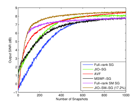
Figure 1: Output SINR versus the number of snapshots

Fig. 2, which includes two experiments, shows the effectiveness of the proposed algorithm with the time-varying bound. The scenario is the same as that in Fig. 1. We compare the full-rank (Fig. 2 (a)) and proposed (Fig. 2 (b)) algorithms with the fixed and time-varying bounds, respectively. In Fig. 2 (a), the one with the fixed bound $\delta=1.0$ shows better performance than that with the time-varying bound but increases the computational cost as a tradeoff ($56.2\%$). The algorithms with higher ($\delta=1.5$) or lower ($\delta=0.7$) bounds exhibit worse convergence and steady-state performance. The same result can be found in Fig. 2 (b) for the proposed algorithm. It indicates that the time-varying bound is capable of improving the performance of the proposed JIO-SM-SG algorithm, while realizing the data-selective updates to reduce the computation complexity.

Figure 2: Output SINR versus the number of snapshots for (a) full-rank SM SG algorithm; (b) JIO-SM-SG algorithm

V Conclusion

In this paper, we employed the time-varying bound SMF technique in the reduced-rank JIO scheme and developed a new adaptive algorithm for the LCMV beamformer. The proposed algorithm retained the positive feature of the iterative exchange of information between the projection matrix and the reduced-rank weight vector, and used data-selective updates to adjust parameters that satisfy the constraints of the LCMV cost function. The variable step sizes in the proposed algorithm provided a way to circumvent the problem between the convergence and misadjustment. It achieved superior performance, especially in large array scenarios, with relatively low complexity.

References

- [1]
- [2] J. Li and P. Stoica, Robust Adaptive Beamforming, Hoboken, NJ: Wiley, 2006.
- [3] O. L. Frost, “An algortihm for linearly constrained adaptive array processing,” IEEE Proc., AP-30, pp. 27-34, 1972.
- [4] H. L. Van Trees, Detection, Estimation, and Modulation, Part IV, Optimum Array Processing,” John Wiley & Sons, 2002.
- [5] S. Haykin, Adaptive Filter Theory, 4rd ed., Englewood Cliffs, NJ: Prentice-Hall, 1996.
- [6] R. C. de Lamare and R. Sampaio-Neto, “Low-complexity variable step-size mechanisms for stochastic gradient algorithms in minimum variance CDMA receivers,” IEEE Trans. Signal Processing, vol. 54, pp. 2302-2317, June 2006.
- [7] L. Wang and R. C. de Lamare, “Constrained adaptive filtering algorithms based on conjugate gradient techniques for beamforming,” IET Signal Processing , vol.4, no.6, pp.686-697, Dec. 2010.
- [8] A. M. Haimovich and Y. Bar-Ness, “An eigenanalysis interference canceler,” IEEE Trans. Signal Processing, vol. 39, pp. 76-84, Jan. 1991.
- [9] D. A. Pados and G. N. Karystinos, “An iterative algorithm for the computation of the MVDR filter,” IEEE Trans. Signal Processing, vol. 49, pp. 290-300, Feb. 2001.
- [10] M. L. Honig and J. S. Goldstein, “Adaptive reduced-rank interference suppression based on the multistage wiener filter,” IEEE Trans. Commun., vol. 50, pp.986-994, Jun. 2002.
- [11] R. C. de Lamare and R. Sampaio-Neto, “Adaptive Reduced-Rank MMSE Filtering with Interpolated FIR Filters and Adaptive Interpolators”, IEEE Sig. Proc. Letters, vol. 12, no. 3, March, 2005.
- [12] R. C. de Lamare and Raimundo Sampaio-Neto, “Reduced-rank Interference Suppression for DS-CDMA based on Interpolated FIR Filters”, IEEE Communications Letters, vol. 9, no. 3, March 2005.
- [13] R. C. de Lamare and R. Sampaio-Neto, “Adaptive Interference Suppression for DS-CDMA Systems based on Interpolated FIR Filters with Adaptive Interpolators in Multipath Channels”, IEEE Transactions on Vehicular Technology, Vol. 56, no. 6, September 2007.
- [14] R. C. de Lamare, “Adaptive reduced-rank LCMV beamforming algorithms based on joint iterative optimisation of filters,” Electronics Letters, vol. 44, pp. 565-566, Apr. 2008.
- [15] R. C. de Lamare, L. Wang, and R. Fa, “Adaptive reduced-rank LCMV beamforming algorithms based on joint iterative optimization of filters: Design and analysis,” Elsevier Signal Processing, vol. 90, pp. 640-652, Feb. 2010.
- [16] W. Chen, U. Mitra, and P. Schniter, “on the equivalence of three reduced rank linear estimators with applications to DS-CDMA,” IEEE Trans. Information Theory, vol. 48, pp. 2609-2614, Sep. 2002.
- [17] P. S. R. Diniz, Adaptive Filtering: Algorithms and Practical Implementations, 3rd ed., Boston, MA: Springer, 2008.
- [18] L. Guo and Y. F. Huang, “Frequency-domain set-membership filtering and its applications,” IEEE Trans. Signal Processing, vol. 55, pp. 1326-1338, Apr. 2007.
- [19] R. C. de Lamare and P. S. R. Diniz, “Set-membership adaptive algorithms based on time-varying error bounds for CDMA interference suppression,” IEEE Trans. Vehicular Technology, vol. 58, pp. 644-654, Feb. 2009.
- [20] L. Guo and Y. F. Huang, “Set-membership adaptive filtering with parameter-dependent error bound tuning,” IEEE Proc. Int. Conf. Acoust. Speech and Sig. Proc., 2005.
- [21] R. C. de Lamare and R. Sampaio-Neto, “Reduced-Rank Adaptive Filtering Based on Joint Iterative Optimization of Adaptive Filters, ” IEEE Signal Processing Letters, Vol. 14 No. 12, December 2007, pp. 980 - 983.
- [22] R. C. de Lamare and R. Sampaio-Neto, “Adaptive Reduced-Rank Processing Based on Joint and Iterative Interpolation, Decimation and Filtering”, IEEE Transactions on Signal Processing, vol. 57, no. 7, July 2009, pp. 2503 - 2514.
- [23] R. Fa, R. C. de Lamare, and L. Wang, “Reduced-Rank STAP Schemes for Airborne Radar Based on Switched Joint Interpolation, Decimation and Filtering Algorithm,” IEEE Transactions on Signal Processing, vol.58, no.8, Aug. 2010, pp.4182-4194.
- [24] R.C. de Lamare, R. Sampaio-Neto, M. Haardt, ”Blind Adaptive Constrained Constant-Modulus Reduced-Rank Interference Suppression Algorithms Based on Interpolation and Switched Decimation,” IEEE Trans. on Signal Processing, vol.59, no.2, pp.681-695, Feb. 2011