On the sphericity test with large-dimensional observations

Abstract

In this paper, we propose corrections to the likelihood ratio test and John’s test for sphericity in large-dimensions. New formulas for the limiting parameters in the CLT for linear spectral statistics of sample covariance matrices with general fourth moments are first established. Using these formulas, we derive the asymptotic distribution of the two proposed test statistics under the null. These asymptotics are valid for general population, i.e. not necessarily Gaussian, provided a finite fourth-moment. Extensive Monte-Carlo experiments are conducted to assess the quality of these tests with a comparison to several existing methods from the literature. Moreover, we also obtain their asymptotic power functions under the alternative of a spiked population model as a specific alternative.

T1Research of this author was partly supported by the National Natural Science Foundation of China (Grant No. 11071213), the Natural Science Foundation of Zhejiang Province (No. R6090034), and the Doctoral Program Fund of Ministry of Education (No. J20110031). t2Research of this author was partly supported by a HKU start-up grant.

and

1 Introduction

Consider a sample $Y_{1},\ldots,Y_{n}$ from a $p$-dimensional multivariate distribution with covariance matrix $\Sigma_{p}$. An important problem in multivariate analysis is to test the sphericity, namely the hypothesis $H_{0}:\Sigma_{p}=\sigma^{2}I_{p}$ where $\sigma^{2}$ is unspecified. If the observations represent a multivariate error with $p$ components, the null hypothesis expresses the fact that the error is cross-sectionally uncorrelated (independent if in addition they are normal) and have a same variance (homoscedasticity).

Much of the existing theory about this test has been exposed first in details in [17] about Gaussian likelihood ratio test and later in [10], [11], [27] and also in textbooks like [18, Chapter 8] and [1, Chapter 10]. Assume for a moment that the sample has a normal distribution with mean zero and covariance matrix $\Sigma_{p}$. Let $S_{n}=n^{-1}\sum_{i}Y_{i}Y_{i}^{*}$ be the sample covariance matrix and denote its eigenvalues by $\{\ell_{i}\}_{1\leq i\leq p}$. Two well established procedures for testing the sphericity are the likelihood ratio test (LRT) and a test devised in [10]. The likelihood ratio statistic is, see e.g. [1, §10.7.2],

$$L_{n}=\left(\frac{(\ell_{1}\cdots\ell_{p})^{1/p}}{\frac{1}{p}(\ell_{1}+\cdots+\ell_{p})}\right)^{\frac{1}{2}pn}\leavevmode\nobreak\ ,$$

which is a power of the ratio of the geometric mean of the sample eigenvalues to the arithmetic mean. It is here noticed that in this formula it is necessary to assume that $p\leq n$ to avoid null eigenvalues in (the numerator of) $L_{n}$. If we let $n\to\infty$ while keeping $p$ fixed, classical asymptotic theory indicates that under the null hypothesis, $-2\log L_{n}\Longrightarrow\chi^{2}_{f}$, a chi-square distribution with degree of freedom $f=\frac{1}{2}p(p+1)-1$. This asymptotic distribution is further refined by the following Box-Bartlett correction (referred as BBLRT):

$$P(-2\rho\log L_{n}\leq x)=P_{f}(x)+\omega_{2}\left\{P_{f+4}(x)-P_{f}(x)\right\}+O(n^{-3})\leavevmode\nobreak\ ,$$ (1.1)

where $P_{k}(x)=P(\chi^{2}_{k}\leq x)$ and

$$\rho=1-\frac{2p^{2}+p+2}{6pn},\qquad\omega_{2}=\frac{(p+2)(p-1)(p-2)(2p^{3}+6p^{2}+3p+2)}{288p^{2}n^{2}\rho^{2}}\leavevmode\nobreak\ .$$

By observing that the asymptotic variance of $-2\log L_{n}$ is proportional to $\mathop{\text{tr}}\{\Sigma(\mathop{\text{tr}}\Sigma)^{-1}-p^{-1}I_{p}\}^{2}$, [10] proposed to use the statistic

$$T_{2}=\frac{p^{2}n}{2}\mathop{\text{tr}}\left\{S_{n}(\mathop{\text{tr}}S_{n})^{-1}-p^{-1}I_{p}\right\}^{2}\leavevmode\nobreak\$$

for testing sphericity. When $p$ is fixed and $n\to\infty$, under the null hypothesis, it also holds that $T_{2}\Longrightarrow\chi^{2}_{f}$, which we referred to as John’s test. It is observed that $T_{2}$ is proportional to the square of the coefficient of variation of the sample eigenvalues, namely

$$T_{2}=\frac{np}{2}\cdot\frac{p^{-1}\sum(\ell_{i}-\overline{\ell})^{2}}{{\overline{\ell}}^{2}}\leavevmode\nobreak\ ,\qquad\text{with\leavevmode\nobreak\ \leavevmode\nobreak\ }\overline{\ell}=\frac{1}{n}\sum_{i}\ell_{i}\leavevmode\nobreak\ .$$

Following the idea of the Box-Bartlett correction, [19] established an expansion for the distribution function of the statistics $T_{2}$ (referred as Nagao’s test),

$$P(T_{2}\leq x) = P_{f}(x)+\frac{1}{n}\left\{a_{p}P_{f+6}(x)+b_{p}P_{f+4}(x)+c_{p}P_{f+2}(x)+d_{p}P_{f}(x)\right\}$$ (1.2)

$$+O(n^{-2}),$$

where

$$a_{p}=\frac{1}{12}(p^{3}+3p^{2}-12-200p^{-1}),\leavevmode\nobreak\ b_{p}=\frac{1}{8}(-2p^{3}-5p^{2}+7p-12-420p^{-1})\leavevmode\nobreak\ ,$$

$$c_{p}=\frac{1}{4}(p^{3}+2p^{2}-p-2-216p^{-1})\leavevmode\nobreak\ ,d_{p}=\frac{1}{24}(-2p^{3}-3p^{2}+p+436p^{-1})\leavevmode\nobreak\ .$$

It has been well known that classical multivariate procedures are in general challenged by large-dimensional data. A small simulation experiment is conducted to explore the performance of the BBLRT and Nagao’s test (two corrections) with growing dimension $p$. The sample size is set to $n=64$ while dimension $p$ increases from 4 to 60 (we have also run other experiments with larger sample sizes $n$ but conclusions are very similar), and the nominal level is set to be $\alpha=0.05$. The samples come from normal vectors with mean zero and identity covariance matrix, and each pair of $(p,n)$ is assessed with 10000 independent replications.

Table 1 gives the empirical sizes of BBLRT and Nagao’s test. It is found here that when the dimension to sample size ratio $p/n$ is below $1/2$, both tests have an empirical size close to the nominal test level $0.05$. Then when the ratio grows up, the BBLRT becomes quickly biased while Nagao’s test still has a correct empirical size. It is striking that although Nagao’s test is derived under classical “$p$ fixed, $n\rightarrow\infty$” regime, it is remarkably robust against dimension inflation.

Table 1: Empirical sizes of BBLRT and Nagao’s test at $5\%$ significance level based on $10000$ independent replications using normal vectors $\mathcal{N}(0,I_{p})$ for $n=64$ and different values of $p$.

$(p,n)$	(4,64)	(8,64)	(16,64)	(32,64)	(48,64)	(56,64)	(60,64)
BBLRT	0.0483	0.0523	0.0491	0.0554	0.1262	0.3989	0.7605
Nagao’s test	0.0485	0.0495	0.0478	0.0518	0.0518	0.0513	0.0495

Therefore, the goal of this paper is to propose novel corrections to both LRT and John’s test to cope with the large-dimensional context. Similar works have already been done in [15], which confirms the robustness of John’s test in large-dimensions; however, these results assume a Gaussian population. In this paper, we remove such a Gaussian restriction, and prove that the robustness of John’s test is in fact general. Following the idea of [15], [9] proposed to use a family of well selected U-statistics to test the sphericity; however, as showed in our simulation study in Section 3, the powers of our corrected John’s test are slightly higher than this test in most cases. More recently, [26] examined the performance of $T_{1}$ (a statistic first put forward in [24]) under non-normality, but with the moment condition $\gamma=3+O(p^{-\epsilon})$, which essentially matches the Gaussian case ($\gamma=3$) asymptotically. We have also removed this moment restriction in our setting. In short, we have unveiled two corrections that have a better performance and removed the Gaussian or nearly Gaussian restriction found in the existing literature.

From the technical point of view, our approach differs from [15] and follows the one devised in [4] and [6]. The central tool is a CLT for linear spectral statistics of sample covariance matrices established in [2] and later refined in [21]. The paper also contains an original contribution on this CLT reported in the Appendix: new formulas for the limiting parameters in the CLT. Since such CLT’s are increasingly important in large-dimensional statistics, we believe that these new formulas will be of independent interest for applications other than those considered in this paper.

The remaining of the paper is organized as follows. Large-dimensional corrections to LRT and John’s test are introduced in Section 2. Section 3 reports a detailed Monte-Carlo study to analyze finite-sample sizes and powers of these two corrections under both normal and non-normal distributed data. Next, Section 4 gives the theoretical analysis of their asymptotic power under the alternative of a spiked population model. Section 5 generalizes our test procedures to populations with an unknown mean. Technical proofs and calculations are relegated to Section 6. The last Section contains some concluding remarks.

2 Large-dimensional corrections

From now on, we assume that the observations $Y_{1},\ldots,Y_{n}$ have the representation $Y_{j}=\Sigma_{p}^{1/2}X_{j}$ where the $p\times n$ table $\{X_{1},\ldots,X_{n}\}=\{x_{ij}\}_{1\leq i\leq p,1\leq j\leq n}$ are made with an array of i.i.d. standardized random variables (mean 0 and variance 1). This setting is motivated by the random matrix theory and it is generic enough for a precise analysis of the sphericity test. Furthermore, under the null hypothesis $H_{0}:\Sigma_{p}=\sigma^{2}I_{p}$ ($\sigma^{2}$ is unspecified), we notice that both LRT and John’s test are independent from the scale parameter $\sigma^{2}$ under the null. Therefore, we can assume w.l.o.g. $\sigma^{2}=1$ when dealing with the null distributions of these test statistics. This will be assumed in all the sections.

Throughout the paper we will use an indicator $\kappa$ set to 2 when $\{x_{ij}\}$ are real and to 1 when they are complex as defined in [3]. Also, we define the kurtosis coefficient $\beta=E|x_{ij}|^{4}-1-\kappa$ for both cases and note that for normal variables, $\beta=0$ (recall that for a standard complex-valued normal random variable, its real and imaginary parts are two iid. $N(0,\frac{1}{2})$ real random variables).

2.1 The corrected likelihood ratio test (CLRT)

For the correction of LRT, let $\mathcal{L}_{n}=-2n^{-1}\log L_{n}\leavevmode\nobreak\$ be the test statistic for $n\geq 1$. Our first main result is the following.

Theorem 2.1.

Assume $\{x_{ij}\}$ are iid, satisfying $Ex_{ij}=0,E|x_{ij}|^{2}=1,E|x_{ij}|^{4}<\infty$. Then under $H_{0}$ and when $\frac{p}{n}=y_{n}\rightarrow y\in(0,1)$,

$$\mathcal{L}_{n}+(p-n)\cdot\log(1-\frac{p}{n})-p$$

$$\Longrightarrow N\{-\frac{\kappa-1}{2}\log(1-y)+\frac{1}{2}\beta y,-\kappa\log(1-y)-\kappa y\}\leavevmode\nobreak\ .$$ (2.1)

The test based on this asymptotic normal distribution will be hereafter referred as the corrected likelihood-ratio test (CLRT). One may observe that the limiting distribution of the test crucially depends on the limiting dimension-to-sample ratio $y$ through the factor $-\log(1-y)$. In particular, the asymptotic variance will blow up quickly when $y$ approaches 1, so it is expected that the power will seriously break down. Monte-Carlo experiments in Section 3 will provide more details on this behavior.

The proof of Theorem 2.1 is based on the following lemma. In all the following, $F^{y}$ denotes the Marčenko-Pastur distribution of index $y$ ($>0$) which is introduced and discussed in the Appendix. And $F^{y}(f(x))=\int f(x)F^{y}(dx)$ denotes the integral of function $f(x)$ with respect to $F^{y}$.

Lemma 2.1.

Let $\{\ell_{i}\}_{1\leq i\leq p}$ be the eigenvalues of the sample covariance matrix $S_{n}=n^{-1}\sum_{i}Y_{i}Y_{i}^{*}$. Then under $H_{0}$ and the conditions of Theorem 2.1, we have

$$\left(\begin{array}[]{cc}\sum_{i=1}^{p}\log\ell_{i}-pF^{y_{n}}(\log x)\\ \sum_{i=1}^{p}\ell_{i}-pF^{y_{n}}(x)\\ \end{array}\right)\Longrightarrow N(\mu_{1},V_{1}),$$

with

$$\mu_{1}=\begin{pmatrix}\frac{\kappa-1}{2}\log(1-y)-\frac{1}{2}\beta y\\ 0\end{pmatrix}\leavevmode\nobreak\ ,$$

and

$$V_{1}=\begin{pmatrix}-\kappa\log(1-y)+\beta y&(\beta+\kappa)y\\ (\beta+\kappa)y&(\beta+\kappa)y\end{pmatrix}\leavevmode\nobreak\ .$$

The proof of this lemma is postponed to Section 6.

Proof.

(of Theorem 2.1).  Let $A_{n}\equiv\sum_{i=1}^{p}\log\ell_{i}-pF^{y_{n}}(\log x)$ and $B_{n}\equiv\sum_{i=1}^{p}\ell_{i}-pF^{y_{n}}(x)$. By Lemma 2.1,

$$\left(\begin{array}[]{cc}A_{n}\\ B_{n}\\ \end{array}\right)\Longrightarrow N(\mu_{1},V_{1}).$$

Consequently, $-A_{n}+B_{n}$ is asymptotically normal with mean $-\frac{\kappa-1}{2}\log(1-y)+\frac{1}{2}\beta y$ and variance

$$V_{1}(1,1)+V_{1}(2,2)-2V_{1}(1,2)=-\kappa\log(1-y)-\kappa y.$$

Besides,

$$\mathcal{L}_{n} = -\Sigma_{i=1}^{p}\log\ell_{i}+p\log(\frac{1}{p}\Sigma_{i=1}^{p}\ell_{i})$$

$$= -(A_{n}+pF^{y_{n}}(\log x))+p\log(\frac{1}{p}(B_{n}+p))$$

$$= -A_{n}-pF^{y_{n}}(\log x)+p\log(1+\frac{B_{n}}{p}).$$

Since $B_{n}\Rightarrow N(0,y(\beta+\kappa))$, $B_{n}=O_{p}(1)$ and $\log(1+{B_{n}}/{p})={B_{n}}/{p}+O_{p}({1}/{p^{2}}).$ Therefore,

$$\mathcal{L}_{n}=-A_{n}-pF^{y_{n}}(\log x)+B_{n}+O_{p}(\frac{1}{p})\leavevmode\nobreak\ .$$

The conclusion follows with the following well-known integrals w.r.t. the Marčenko-Pastur distribution $F^{y}$ ($y<1$) in [2],

$$F^{y}(\log x)=\frac{y-1}{y}\log(1-y)-1\leavevmode\nobreak\ ,\quad F^{y}(x)=1.$$

The proof of Theorem 2.1 is complete. ∎

2.2 The corrected John’s test (CJ)

Earlier than the asymptotic expansion (1.2) given in [19], [10] proved that when the observations are normal, the sphericity test based on $T_{2}$ is a locally most powerful invariant test. It is also established in [11] that under these conditions, the limiting distribution of $T_{2}$ under $H_{0}$ is $\chi^{2}_{f}$ with degree of freedom $f=\frac{1}{2}p(p+1)-1$, or equivalently,

$$nU-p\Longrightarrow\frac{2}{p}\chi^{2}_{f}-p\leavevmode\nobreak\ ,$$

where for convenience, we have let $U=2(np)^{-1}T_{2}$. Clearly, this limit has been established for $n\to\infty$ and a fixed dimension $p$. However, if we now let $p\to\infty$ in the right-hand side of the above result, it is not hard to see that $\frac{2}{p}\chi^{2}_{f}-p$ will tend to the normal distribution $N(1,4)$. It then seems “natural” to conjecture that when both $p$ and $n$ grow to infinity in some “proper” way, it may happen that

$$nU-p\Longrightarrow N(1,4)\leavevmode\nobreak\ .$$ (2.2)

This is indeed the main result of [15] where this asymptotic distribution was established assuming that data are normal-distributed and $p$ and $n$ grow to infinity in a proportional way (i.e. $p/n\to y>0$).

In this section, we provide a more general result using our own approach. In particular, the distribution of the observation is arbitrary provided a finite fourth moment exists.

Theorem 2.2.

Assume $\{x_{ij}\}$ are iid, satisfying $Ex_{ij}=0,E|x_{ij}|^{2}=1,E|x_{ij}|^{4}<\infty$, and let $U=2(np)^{-1}T_{2}$ be the test statistic. Then under $H_{0}$ and when $p\rightarrow\infty,n\rightarrow\infty,\frac{p}{n}=y_{n}\rightarrow y\in(0,\infty)$,

$$nU-p\Longrightarrow N(\kappa+\beta-1,2\kappa)\leavevmode\nobreak\ .$$ (2.3)

The test based on the asymptotic normal distribution given in equation (2.3) will be hereafter referred as the corrected John’s test (CJ).

A striking fact in this theorem is that as in the normal case, the limiting distribution of CJ is independent of the dimension-to-sample ratio $y=\lim p/n$. In particular, the limiting distribution derived under classical scheme ($p$ fixed, $n\rightarrow\infty$), e.g. the distribution $\frac{2}{p}\chi_{f}^{2}-p$ in the normal case, when used for large $p$, stays very close to this limiting distribution derived for large-dimensional scheme ($p\rightarrow\infty,n\rightarrow\infty,p/n\rightarrow y\in(0,\infty)$). In this sense, Theorem 2.2 gives a theoretic explanation to the widely observed robustness of John’s test against the dimension inflation. Moreover, CJ is also valid for the $p$ larger (or much larger) than $n$ case in contrast to the CLRT where this ratio should be kept smaller than 1 to avoid null eigenvalues.

It is also worth noticing that for real normal data, we have $\kappa=2$ and $\beta=0$ so that the theorem above reduces to $nU-p\Rightarrow N(1,4)$. This is exactly the result discussed in [15]. Besides, if the data has a non-normal distribution but has the same first four moments as the normal distribution, we have again $nU-p\Rightarrow N(1,4)$, which turns out to have a universality property.

The proof of Theorem 2.2 is based on the following lemma.

Lemma 2.2.

Let $\{\ell_{i}\}_{1\leq i\leq p}$ be the eigenvalues of the sample covariance matrix $S_{n}=n^{-1}\sum_{i}Y_{i}Y_{i}^{*}$. Then under $H_{0}$ and the conditions of Theorem 2.2, we have

$$\left(\begin{array}[]{cc}\sum_{i=1}^{p}\ell_{i}^{2}-p(1+y_{n})\\ \sum_{i=1}^{p}\ell_{i}-p\\ \end{array}\right)\Longrightarrow N(\mu_{2},V_{2}),$$

with

$$\mu_{2}=\begin{pmatrix}(\kappa-1+\beta)y\\ 0\end{pmatrix}\leavevmode\nobreak\ ,$$

and

$$V_{2}=\begin{pmatrix}2\kappa y^{2}+4(\kappa+\beta)(y+2y^{2}+y^{3})&2(\kappa+\beta)(y+y^{2})\\ 2(\kappa+\beta)(y+y^{2})&(\kappa+\beta)y\end{pmatrix}\leavevmode\nobreak\ .$$

The proof of this lemma is postponed to Section 6.

Proof.

(of Theorem 2.2). The result of Lemma 2.2 can be rewritten as:

$$n\left(\begin{array}[]{cc}p^{-1}\sum_{i=1}^{p}\ell_{i}^{2}-1-\frac{p}{n}-\frac{(\kappa+\beta-1)y}{p}\\ p^{-1}\sum_{i=1}^{p}\ell_{i}-1\end{array}\right)\Longrightarrow N\Bigg{(}\left(\begin{array}[]{cc}0\\ 0\end{array}\right),\ \frac{1}{y^{2}}\cdot V_{2}\Bigg{)}.$$

Define the function $f(x,y)=\frac{x}{y^{2}}-1$, then $U=f(p^{-1}\Sigma_{i=1}^{p}\ell_{i}^{2},\leavevmode\nobreak\ p^{-1}\Sigma_{i=1}^{p}\ell_{i})$.

We have

$$\frac{\partial f}{\partial x}(1+\frac{p}{n}+\frac{(\kappa+\beta-1)y}{p},1)=1\leavevmode\nobreak\ ,$$

$$\frac{\partial f}{\partial y}(1+\frac{p}{n}+\frac{(\kappa+\beta-1)y}{p},1)=-2(1+\frac{p}{n}+\frac{(\kappa+\beta-1)y}{p})\leavevmode\nobreak\ ,$$

$$f(1+\frac{p}{n}+\frac{(\kappa+\beta-1)y}{p},1)=\frac{p}{n}+\frac{(\kappa+\beta-1)y}{p}\leavevmode\nobreak\ .$$

By the delta method,

$$n\Big{(}U-f(1+\frac{p}{n}+\frac{(\kappa+\beta-1)y}{p},1)\Big{)}\Longrightarrow N(0,\lim C),$$

where
$C=$$\left(\begin{array}[]{cc}\frac{\partial f}{\partial x}(1+\frac{p}{n}+\frac{(\kappa+\beta-1)y}{p},1)\\ \frac{\partial f}{\partial y}(1+\frac{p}{n}+\frac{(\kappa+\beta-1)y}{p},1)\\ \end{array}\right)^{T}\$$\cdot\Big{(}\frac{1}{y^{2}}V_{2}\Big{)}\cdot$$\left(\begin{array}[]{cc}\frac{\partial f}{\partial x}(1+\frac{p}{n}+\frac{(\kappa+\beta-1)y}{p},1)\\ \frac{\partial f}{\partial y}(1+\frac{p}{n}+\frac{(\kappa+\beta-1)y}{p},1)\\ \end{array}\right)\$

$\longrightarrow 2\kappa\leavevmode\nobreak\ .$

Therefore,

$$n(U-\frac{p}{n}-\frac{(\kappa+\beta-1)y}{p})\Longrightarrow N(0,2\kappa)\leavevmode\nobreak\ ,$$

that is,

$$nU-p\Longrightarrow N(\kappa+\beta-1,2\kappa)\leavevmode\nobreak\ .$$

The proof of Theorem 2.2 is complete. ∎

Remark 2.1.

Note that in Theorems 2.1 and 2.2 appears the parameter $\beta$, which is in practice unknown with real data. So we may estimate the parameter $\beta$ using the fourth-order sample moment:

$$\widehat{\beta}=\frac{1}{np}\sum_{i=1}^{p}\sum_{j=1}^{n}|Y_{j}(i)|^{4}-\kappa-1\leavevmode\nobreak\ .$$

According to the law of large numbers, $\hat{\beta}=\beta+o_{p}(1)$, so substituting $\hat{\beta}$ for $\beta$ in Theorems 2.1 and 2.2 does not modify the limiting distribution.

3 Monte Carlo study

Monte Carlo simulations are conducted to find empirical sizes and powers of CLRT and CJ. In particular, here we want to examine the following questions: how robust are the tests against non-normal distributed data and what is the range of the dimension to sample ratio $p/n$ where the tests are applicable.

For comparison, we show both the performance of the LW test using the asymptotic $N(1,4)$ distribution in (2.2) (Notice however this is the CJ test under normal distribution) and the Chen’s test (denoted as C for short) using the asymptotic $N(0,4)$ distribution derived in [9]. The nominal test level is set to be $\alpha=0.05$, and for each pair of $(p,n)$, we run 10000 independent replications.

We consider two scenarios with respect to the random vectors $Y_{i}$ :

1. $Y_{i}$ is $p$-dimensional real random vector from the multivariate normal population ${\mathcal{N}}(0,I_{p})$. In this case, $\kappa=2$ and $\beta=0$.

2. $Y_{i}$ consists of iid real random variables with distribution $Gamma(4,2)-2$ so that $y_{ij}$ satisfies $Ey_{ij}=0,Ey_{ij}^{4}=4.5$. In this case, $\kappa=2$ and $\beta=1.5$.

Table 2: Empirical sizes of LW, CJ, CLRT and C test at $5\%$ significance level based on 10000 independent applications with real $N(0,1)$ random variables and with real Gamma(4,2)-2 random variables.

$(p,n)$		$N(0,1)$					Gamma(4,2)-2
		LW/CJ	CLRT	C			LW	CLRT	CJ	C
(4,64)		0.0498	0.0553	0.0523			0.1396	0.074	0.0698	0.0717
(8,64)		0.0545	0.061	0.0572			0.1757	0.0721	0.0804	0.078
(16,64)		0.0539	0.0547	0.0577			0.1854	0.0614	0.078	0.0756
(32,64)		0.0558	0.0531	0.0612			0.1943	0.0564	0.0703	0.0682
(48,64)		0.0551	0.0522	0.0602			0.1956	0.0568	0.0685	0.0652
(56,64)		0.0547	0.0505	0.0596			0.1942	0.0549	0.0615	0.0603
(60,64)		0.0523	0.0587	0.0585			0.194	0.0582	0.0615	0.0603
(8,128)		0.0539	0.0546	0.0569			0.1732	0.0701	0.075	0.0754
(16,128)		0.0523	0.0534	0.0548			0.1859	0.0673	0.0724	0.0694
(32,128)		0.051	0.0545	0.0523			0.1951	0.0615	0.0695	0.0693
(64,128)		0.0538	0.0528	0.0552			0.1867	0.0485	0.0603	0.0597
(96,128)		0.055	0.0568	0.0581			0.1892	0.0539	0.0577	0.0579
(112,128)		0.0543	0.0522	0.0591			0.1875	0.0534	0.0591	0.0593
(120,128)		0.0545	0.0541	0.0561			0.1849	0.051	0.0598	0.0596
(16,256)		0.0544	0.055	0.0574			0.1898	0.0694	0.0719	0.0716
(32,256)		0.0534	0.0515	0.0553			0.1865	0.0574	0.0634	0.0614
(64,256)		0.0519	0.0537	0.0522			0.1869	0.0534	0.0598	0.0608
(128,256)		0.0507	0.0505	0.0498			0.1858	0.051	0.0555	0.0552
(192,256)		0.0507	0.054	0.0518			0.1862	0.0464	0.052	0.0535
(224,256)		0.0503	0.0541	0.0516			0.1837	0.0469	0.0541	0.0538
(240,256)		0.0494	0.053	0.0521			0.1831	0.049	0.0533	0.0559
(32,512)		0.0542	0.0543	0.0554			0.1884	0.0571	0.0606	0.059
(64,512)		0.0512	0.0497	0.0513			0.1816	0.0567	0.0579	0.0557
(128,512)		0.0519	0.0567	0.0533			0.1832	0.0491	0.0507	0.0504
(256,512)		0.0491	0.0503	0.0501			0.1801	0.0504	0.0495	0.0492
(384,512)		0.0487	0.0505	0.0499			0.1826	0.051	0.0502	0.0507
(448,512)		0.0496	0.0495	0.0503			0.1881	0.0526	0.0482	0.0485
(480,512)		0.0488	0.0511	0.0505			0.1801	0.0523	0.053	0.0516

Table 2 reports the sizes of the four tests in these two scenarios for different values of $(p,n)$. We see that when $\{y_{ij}\}$ are normal, LW (=CJ), CLRT and C all have similar empirical sizes tending to the nominal level 0.05 as either $p$ or $n$ increases. But when $\{y_{ij}\}$ are Gamma-distributed, the sizes of LW are higher than 0.1 no matter how large the values of $p$ and $n$ are while the sizes of CLRT and CJ all converge to the nominal level 0.05 as either $p$ or $n$ gets larger. This empirically confirms that normal assumptions are needed for the result of [15] while our corrected statistics CLRT and CJ (also the C test) have no such distributional restriction.

As for empirical powers, we consider two alternatives (here, the limiting spectral distributions of $\Sigma_{p}$ under these two alternatives differs from that under $H_{0}$):

1. $\Sigma_{p}$ is diagonal with half of its diagonal elements 0.5 and half 1. We denote its power by Power 1 ;

2. $\Sigma_{p}$ is diagonal with 1/4 of the elements equal 0.5 and 3/4 equal 1. We denote its power by Power 2 .

Table 3 reports the powers of LW(=CJ), CLRT and C when $\{y_{ij}\}$ are distributed as $N(0,1)$, and of CJ, CLRT and C when $\{y_{ij}\}$ are distributed as Gamma(4,2)-2, for the situation when $n$ equals $64$ or $128$, with varying values of $p$ and under the above mentioned two alternatives. For $n=256$ and $p$ varying from 16 to 240, all the tests have powers around 1 under both alternatives so that these values are omitted. And in order to find the trend of these powers, we also present the results when $n=128$ in Figure 1 and Figure 2.

Table 3: Empirical powers of LW, CJ, CLRT and C test at $5\%$ significance level based on 10000 independent applications with real $N(0,1)$ random variables and with real Gamma(4,2)-2 random variables under two alternatives Power 1 and 2 (see the text for details).

$N(0,1)$
$(p,n)$		Power 1					Power 2
		LW/CJ	CLRT	C			LW/CJ	CLRT	C
(4,64)		0.7754	0.7919	0.772			0.4694	0.6052	0.4716
(8,64)		0.8662	0.8729	0.8582			0.5313	0.6756	0.5308
(16,64)		0.912	0.9075	0.9029			0.5732	0.6889	0.5671
(32,64)		0.9384	0.8791	0.931			0.5868	0.6238	0.5775
(48,64)		0.9471	0.7767	0.9389			0.6035	0.5036	0.5982
(56,64)		0.949	0.6663	0.9411			0.6025	0.4055	0.5982
(60,64)		0.9501	0.5575	0.941			0.6048	0.3328	0.5989
(8,128)		0.9984	0.9989	0.9986			0.9424	0.9776	0.9391
(16,128)		0.9998	1	0.9998			0.9698	0.9926	0.9676
(32,128)		1	1	1			0.9781	0.9956	0.9747
(64,128)		1	1	1			0.9823	0.9897	0.9788
(96,128)		1	0.9996	1			0.9824	0.9532	0.9804
(112,128)		1	0.9943	1			0.9841	0.881	0.9808
(120,128)		1	0.9746	1			0.9844	0.7953	0.9817
$Gamma(4,2)-2$
$(p,n)$		Power 1					Power 2
		CJ	CLRT	C			CJ	CLRT	C
(4,64)		0.6517	0.6826	0.6628			0.3998	0.5188	0.4204
(8,64)		0.7693	0.7916	0.781			0.4757	0.5927	0.4889
(16,64)		0.8464	0.8439	0.846			0.5327	0.633	0.5318
(32,64)		0.9041	0.848	0.9032			0.5805	0.5966	0.5667
(48,64)		0.9245	0.7606	0.924			0.5817	0.4914	0.5804
(56,64)		0.9267	0.6516	0.9247			0.5882	0.4078	0.583
(60,64)		0.9288	0.5547	0.9257			0.5919	0.3372	0.5848
(8,128)		0.9859	0.9875	0.9873			0.8704	0.9294	0.8748
(16,128)		0.999	0.999	0.9987			0.9276	0.9699	0.9311
(32,128)		0.9999	1	0.9999			0.9582	0.9873	0.9587
(64,128)		1	0.9998	1			0.9729	0.984	0.9727
(96,128)		1	0.999	1			0.9771	0.9482	0.9763
(112,128)		1	0.9924	1			0.9781	0.8747	0.9763
(120,128)		1	0.9728	1			0.9786	0.7864	0.977

The behavior of Power 1 and Power 2 in each figure related to the three statistics are similar, except that Power 1 is much higher compared with Power 2 for a given dimension design $(p,n)$ and any given test for the reason that the first alternative differs more from the null than the second one. The powers of LW (in the normal case), CJ (in the Gamma case) and C are all monotonically increasing in $p$ for a fixed value of $n$. But for CLRT, when $n$ is fixed, the powers first increase in $p$ and then become decreasing when $p$ is getting close to $n$. This can be explained by the fact that when $p$ is close to $n$, some of the eigenvalues of $S_{n}$ are getting close to zero, causing the CLRT nearly degenerate and losing power.

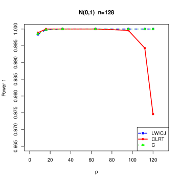
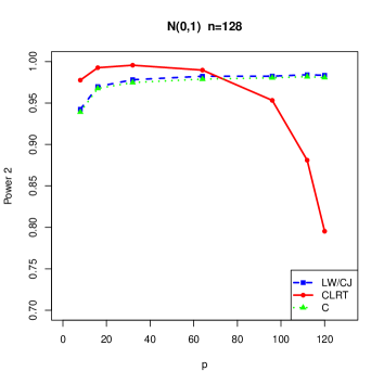
Figure 1: Empirical powers of LW/CJ, CLRT and C test at $5\%$ significance level based on 10000 independent applications with real N(0,1) random variables for fixed $n=128$ under two alternatives Power 1 and 2 (see the text for details).

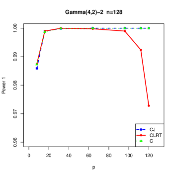
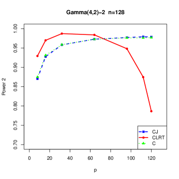
Figure 2: Empirical powers of CJ, CLRT and C test at $5\%$ significance level based on 10000 independent applications with real Gamma(4,2)-2 random variables for fixed $n=128$ under two alternatives Power 1 and 2 (see the text for details).

Besides, we find that in the normal case the trend of C’s power is very much alike of those of LW while in the Gamma case it is similar with those of CJ under both alternatives. And in most of the cases (especially in large $p$ case), the power of C test is slightly lower than LW (in the normal case) and CJ (in the Gamma case).

Lastly, we examine the performance of CJ and C when $p$ is larger than $n$. Empirical sizes and powers are presented in Table 4. We choose the variables to be distributed as Gamma(4,2)-2 since CJ reduces to LW in the normal case, and [15] has already reported the performance of LW when $p$ is larger than $n$. From the table, we see that when $p$ is larger than $n$, the size of CJ is still correct and it is always around the nominal level 0.05 as the dimension $p$ increases and the same phenomenon exists for C test.

Table 4: Empirical sizes and powers (Power 1 and 2) of CJ test and C test at $5\%$ significance level based on 10000 independent applications with real Gamma(4,2)-2 random variables when $p\geq n$.

$(p,n)$		CJ					C
		Size	Power 1	Power 2			Size	Power 1	Power 2
(64,64)		0.0624	0.9282	0.5897			0.0624	0.9257	0.5821
(320,64)		0.0577	0.9526	0.612			0.0576	0.9472	0.6059
(640,64)		0.0558	0.959	0.6273			0.0562	0.9541	0.6105
(960,64)		0.0543	0.9631	0.6259			0.0551	0.955	0.6153
(1280,64)		0.0555	0.9607	0.6192			0.0577	0.9544	0.6067

When we evaluate the power, the same two alternatives Power 1 and Power 2 as above are considered. The sample size is fixed to $n=64$ and the ratio $p/n$ varies from 1 to 20. We see that Power 1 are much higher than Power 2 for the same reason that the first alternative is easier to be distinguished from $H_{0}$. Besides, the powers under both alternatives all increase monotonically for $1\leq\frac{p}{n}\leq 15$. However, when $p/n$ is getting larger, say $p/n=20$, we can observe that its size is a little larger and powers a little drop (compared with $p/n=15$) but overall, it still behaves well, which can be considered as free from the assumption constraint “$p/n\rightarrow y$”. Besides, the powers of CJ are always slightly higher than those of C in this “large $p$ small $n$” setting.

Since the asymptotic distribution for the CLRT and CJ are both derived under the “Marcenko-Pasture scheme” (i.e $p/n\rightarrow y\in(0,\infty)$), if $p/n$ is getting too large ($p\gg n$), it seems that the limiting results provided in this paper will loose accuracy. It is worth noticing that [7] has extended the LW test to such a scheme ($p\gg n$) for multivariate normal distribution.

Summarizing all these findings from this Monte-Carlo study, the overall figure is the following: when the ratio $p/n$ is much lower than 1 (say smaller than 1/2), it is preferable to employ CLRT (than CJ, LW or C); while this ratio is higher, CJ (or LW for normal data) becomes more powerful (slightly more powerful than C).

4 Asymptotic powers: under the spiked population alternative

In this section, we give an analysis of the powers of the two corrections: CLRT and CJ. To this end, we consider an alternative model that has attracted lots of attention since its introduction by [13], namely, the spiked population model. This model can be described as follows: the eigenvalues of $\Sigma_{p}$ are all one except for a few fixed number of them. Thus, we restrict our sphericity testing problem to the following:

$$H_{0}:\Sigma_{p}=I_{p}\leavevmode\nobreak\ \leavevmode\nobreak\ \leavevmode\nobreak\ vs\leavevmode\nobreak\ \leavevmode\nobreak\ \leavevmode\nobreak\ H_{1}^{*}:\Sigma_{p}=diag(\underbrace{a_{1},\cdots,a_{1}}_{n_{1}},\cdots,\underbrace{a_{k},\cdots,a_{k}}_{n_{k}},\underbrace{1,\cdots,1}_{p-M}),$$

where the multiplicity numbers $n_{i}$’s are fixed and satisfying $n_{1}+\cdots+n_{k}=M$. We derive the explicit expressions of the power functions of CLRT and CJ in this section.

Under $H_{1}^{*}$, the empirical spectral distribution of $\Sigma_{p}$ is

$$H_{n}=\frac{1}{p}\sum_{i=1}^{k}n_{i}\delta_{a_{i}}+\frac{p-M}{p}\delta_{1}\leavevmode\nobreak\ ,$$ (4.1)

and it will converge to $\delta_{1}$, a Dirac mass at 1, which is the same as the limit under the null hypothesis $H_{0}:\Sigma_{p}=I_{p}$. From this point of view, anything related to the limiting spectral distribution remains the same whenever under $H_{0}$ or $H_{1}^{*}$. Then recall the CLT for LSS of the sample covariance matrix, as provided in [2], is of the form:

$$p\int f(x)d(F^{S_{n}}(x)-F^{y_{n}}(x))\Longrightarrow N(\mu,\sigma^{2})\leavevmode\nobreak\ ,$$

where the right side of this equation is determined only by the limiting spectral distribution. So we can conclude that the limiting parameters $\mu$ and $\sigma^{2}$ remain the same under $H_{0}$ and $H_{1}^{*}$, only the centering term $p\int f(x)dF^{y_{n}}(x)$ possibly makes a difference. Since there’s a $p$ in front of $\int f(x)dF^{y_{n}}(x)$, which tends to infinity as assumed, so knowing the convergence $H_{n}\rightarrow\delta_{1}$ is not enough and more details about the convergence are needed. In [28], we have established an asymptotic expansion for the centering parameter when the population has a spiked structure. We will use these formulas like equations (4.2), (4.3) and (4.6) in the following to derive the powers of the CLRT and CJ.

Lemma 2.1 remains the same under $H_{1}^{*}$, except that this time the centering terms become (see formulas (4.11) and (4.12) in [28]):

$$F^{y_{n}}(\log x)=\frac{1}{p}\sum_{i=1}^{k}n_{i}\log a_{i}-1+(1-\frac{1}{y_{n}})\log(1-y_{n})+O(\frac{1}{p^{2}})\leavevmode\nobreak\ ,$$ (4.2)

$$F^{y_{n}}(x)=1+\frac{1}{p}\sum_{i=1}^{k}n_{i}a_{i}-\frac{M}{p}+O(\frac{1}{p^{2}})\leavevmode\nobreak\ .$$ (4.3)

Repeating the proof of Theorem 2.1, we can get:

$$\mathcal{L}_{n}-p+(p-n)\log(1-\frac{p}{n})+\sum_{i=1}^{k}n_{i}\big{(}\log a_{i}-a_{i}+1\big{)}$$

$$\Longrightarrow N\Big{(}-\frac{\kappa-1}{2}\log(1-y)+\frac{1}{2}\beta y\leavevmode\nobreak\ ,\leavevmode\nobreak\ -\kappa\log(1-y)-\kappa y\Big{)}$$ (4.4)

under $H_{1}^{*}$. As a result, the power of CLRT for testing $H_{0}$ against $H_{1}^{*}$ can be expressed as:

$$\beta_{1}(\alpha)=1-\Phi\bigg{(}\Phi^{-1}(1-\alpha)-\frac{\sum_{i=1}^{k}n_{i}\big{(}a_{i}-\log a_{i}-1\big{)}}{\sqrt{-\kappa\log(1-y)-\kappa y}}\bigg{)}\leavevmode\nobreak\$$ (4.5)

for a pre-given significance level $\alpha$.

It is worth noticing here that if the alternative has only one simple spike, i.e. $k=1,\leavevmode\nobreak\ n_{k}=1$, and assuming the real Gaussian variable case, i.e. $\kappa=2$, (4.5) reduces to a result provided in [20]. However, our formula is valid for a general number of spikes with eventual multiplicities. Besides, these authors use some more sophisticated tools of asymptotic contiguity and Le Cam’s first and third lemmas, which are totally different from ours.

In order to calculate the power function of CJ, we restated Lemma 2.2 as follows:

$$\left(\begin{array}[]{cc}\sum_{i=1}^{p}l_{i}^{2}-pF^{y_{n}}(x^{2})\\ \sum_{i=1}^{p}l_{i}-pF^{y_{n}}(x)\\ \end{array}\right)\Longrightarrow N(\mu_{2},V_{2})\leavevmode\nobreak\ ,$$

where

$$F^{y_{n}}(x^{2})=\frac{2}{n}\sum_{i=1}^{k}n_{i}a_{i}-\frac{2}{n}M+1+y_{n}-\frac{M}{p}+\frac{1}{p}\sum_{i=1}^{k}n_{i}a_{i}^{2}+O(\frac{1}{p^{2}}),$$ (4.6)

$$F^{y_{n}}(x)=1+\frac{1}{p}\sum_{i=1}^{k}n_{i}a_{i}-\frac{M}{p}+O(\frac{1}{p^{2}})\leavevmode\nobreak\ .$$

Using the delta method as in the proof of Theorem 2.2, this time, we have

$$nU-p-\frac{n}{p}\sum_{i=1}^{k}n_{i}(a_{i}-1)^{2}\Longrightarrow N(\kappa+\beta-1,2\kappa)$$ (4.7)

under $H_{1}^{*}$.

Power function of CJ can be expressed as

$$\beta_{2}(\alpha)=1-\Phi\bigg{(}\Phi^{-1}(1-\alpha)-\frac{n}{p}\cdot\frac{\sum_{i=1}^{k}n_{i}(a_{i}-1)^{2}}{\sqrt{2\kappa}}\bigg{)}\leavevmode\nobreak\$$ (4.8)

for a pre-given significance level $\alpha$.

Now consider the functions $a_{i}-\log a_{i}-1$ and $(a_{i}-1)^{2}$ appearing in the expressions (4.5) and (4.8), they will achieve their minimum value $0$ at $a_{i}=1$, which is to say, once $a_{i}$’s going away from 1, the powers $\beta_{1}(\alpha)$ and $\beta_{2}(\alpha)$ will both increase. This phenomenon agrees with our intuition, since the more $a_{i}$’s deviate away from 1, the easier to distinguish $H_{0}$ from $H_{1}^{*}$. Therefore, the powers should naturally grow higher.

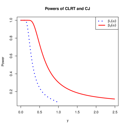
Figure 3: Theoretical powers of CLRT ($\beta_{1}(\alpha)$) and CJ ($\beta_{2}(\alpha)$) under the spiked population alternative.

Then, we consider the power functions $\beta_{1}(\alpha)$ and $\beta_{2}(\alpha)$ as functions of $y$, and see how they are going along with $y^{\prime}s$ changing. we see that in expression (4.5), $\sqrt{-\log(1-y)-y}$ is increasing when $y\in(0,1)$, so $\beta_{1}(\alpha)$ is decreasing as the function of $y$, which attains its maximum value $1$ when $y\rightarrow 0_{+}$ and minimum value $\alpha$ when $y\rightarrow 1_{-}$. Also, expression (4.8) is obviously a decreasing function of $y$, attaining its maximum value $1$ when $y\rightarrow 0_{+}$ and minimum value $\alpha$ when $y\rightarrow+\infty$. We present the trends of $\beta_{1}(\alpha)$ and $\beta_{2}(\alpha)$ (corresponding to the power of CLRT and CJ) in Figure 3 when only one spike $a=2.5$ exists. It is however a little different from the non-spiked case as showed in the simulation in Section 3 (both Figure 1 and Figure 2), where the power of CLRT first increases then decreases while the power of CJ is always increasing along with the increase of the value of $p$. These power drops are due to the fact that when $p$ increases, since only one spike eigenvalue is considered, it becomes harder to distinguish both hypotheses. Besides, an interesting finding here is that these power functions give a new confirmation of the fact that CLRT behaves quite badly when $y\rightarrow 1_{-}$, while CJ test has a reasonable power for a significant range of $y>1$.

5 Generalization to the case when the population mean is unknown

So far, we have assumed the observation $(Y_{i})$ are centered. However, this is hardly true in practical situations when $\mu=EY_{i}$ is usually unknown. Therefore, the sample covariance matrix should be taken as

$$S_{n}^{*}=\frac{1}{n-1}\sum_{i=1}^{n}(Y_{i}-\overline{Y})(Y_{i}-\overline{Y})^{*}\leavevmode\nobreak\ ,$$

where $\overline{Y}=\frac{1}{n}\sum_{i=1}^{n}Y_{i}$ is the sample mean. Because $\overline{Y}\overline{Y}^{*}$ is a rank one matrix, substituting $S_{n}$ for $S_{n}^{*}$ when $\mu$ is unknown will not affect the limiting distribution in the CLT for LSS; while it is not the case for the centering parameter, for it has a $p$ in front.

Recently, [22] shows that if we use $S_{n}^{*}$ in the CLT for LSS when $\mu$ is unknown, the limiting variance remains the same as we use $S_{n}$; while the limiting mean has a shift which can be expressed as a complex contour integral. Later, [30] looks into this shift and finally derives a concise conclusion on the CLT corresponding to $S_{n}^{*}$: the random vector $\big{(}X_{n}^{*}(f_{1}),\cdots,X_{n}^{*}(f_{k})\big{)}$ converges weakly to a Gaussian vector with the same mean and covariance function as given in Theorem A.1, where this time, $X_{n}^{*}(f)=p\int f(x)d(F^{S_{n}^{*}}-F^{y_{n-1}})$. It is here important to pay attention that the only difference is in the centering term, where we use the new ratio $y_{n-1}=\frac{p}{n-1}$ instead of the previous $y_{n}=\frac{p}{n}$, while leaving all the other terms unchanged.

Using this result, we can modify our Theorems 2.1 and 2.2 to get the CLT of CLRT and CJ under $H_{0}$ when $\mu$ is unknown only by considering the eigenvalues of $S_{n}^{*}$ and substituting $n-1$ for $n$ in the centering terms. More precisely, now equations (2.1) and (2.3) in Theorems 2.1 and 2.2 become

$$\mathcal{L}_{n}+(p-n+1)\cdot\log(1-\frac{p}{n-1})-p$$

$$\Longrightarrow N\{-\frac{\kappa-1}{2}\log(1-y)+\frac{1}{2}\beta y,-\kappa\log(1-y)-\kappa y\}\leavevmode\nobreak\$$

and

$$nU-\frac{np}{n-1}\Longrightarrow N(\kappa+\beta-1,2\kappa)\leavevmode\nobreak\ .$$

The same procedures can be applied to get the CLT of CLRT and CJ under $H_{1}^{*}$ when $\mu$ is unknown. This time, equations (4) and (4.7) become

$$\mathcal{L}_{n}-p+(p-n+1)\log(1-\frac{p}{n-1})+\sum_{i=1}^{k}n_{i}\big{(}\log a_{i}-a_{i}+1\big{)}$$

$$\Longrightarrow N\Big{(}-\frac{\kappa-1}{2}\log(1-y)+\frac{1}{2}\beta y\leavevmode\nobreak\ ,\leavevmode\nobreak\ -\kappa\log(1-y)-\kappa y\Big{)}$$

and

$$nU-\frac{np}{n-1}-\frac{n}{p}\sum_{i=1}^{k}n_{i}(a_{i}-1)^{2}\Longrightarrow N(\kappa+\beta-1,2\kappa)\leavevmode\nobreak\ ,$$

and therefore the powers of CLRT and CJ under the spiked alternative remain unchanged as expressed in (4.5) and (4.8).

.

6 Additional proofs

We recall these two important formulas which appear in the Appendix as (A.2) and (A.3) here for the convenience of reading:

$$\mathbb{E}[X_{f}] = (\kappa-1)I_{1}(f)+\beta I_{2}(f)\leavevmode\nobreak\ ,$$

$$\mathop{\text{Cov}}(X_{f},X_{g}) = \kappa J_{1}(f,g)+\beta J_{2}(f,g)\leavevmode\nobreak\ .$$

6.1 Proof of Lemma 2.1

Let for $x>0$, $f(x)=\log x$ and $g(x)=x$. Define $A_{n}$ and $B_{n}$ by the decompositions

$$\sum_{i=1}^{p}\log\ell_{i} = p\int f(x)d(F_{n}(x)-F^{y_{n}}(x))+pF^{y_{n}}(f)=A_{n}+pF^{y_{n}}(f)\leavevmode\nobreak\ ,$$

$$\sum_{i=1}^{p}\ell_{i} = p\int g(x)d(F_{n}(x)-F^{y_{n}}(x))+pF^{y_{n}}(g)=B_{n}+pF^{y_{n}}(g)\leavevmode\nobreak\ .$$

Applying Theorem A.1 given in the Appendix to the pair $(f,g)$, we have

$$\left(\begin{array}[]{cc}A_{n}\\ B_{n}\end{array}\right)\Longrightarrow N\Bigg{(}\left(\begin{array}[]{cc}EX_{f}\\ EX_{g}\end{array}\right),\ \left(\begin{array}[]{cc}\mathop{\text{Cov}}(X_{f},X_{f})&\mathop{\text{Cov}}(X_{f},X_{g})\\ \mathop{\text{Cov}}(X_{g},X_{f})&\mathop{\text{Cov}}(X_{g},X_{g})\end{array}\right)\ \Bigg{)}.$$

It remains to evaluate the limiting parameters and this results from the following calculations where $h$ is denoted as $\sqrt{y}$:

$$I_{1}(f,r) = \frac{1}{2}\log\left(1-h^{2}/r^{2}\right)\leavevmode\nobreak\ ,$$ (6.1)

$$I_{1}(g,r) = 0\leavevmode\nobreak\ ,$$ (6.2)

$$I_{2}(f) = -\frac{1}{2}h^{2}\leavevmode\nobreak\ ,$$ (6.3)

$$I_{2}(g) = 0\leavevmode\nobreak\ ,$$ (6.4)

$$J_{1}(f,g,r) = \frac{h^{2}}{r^{2}}\leavevmode\nobreak\ ,$$ (6.5)

$$J_{1}(f,f,r) = -\frac{1}{r}\log(1-h^{2}/r)\leavevmode\nobreak\ ,$$ (6.6)

$$J_{1}(g,g,r) = \frac{h^{2}}{r^{2}}\leavevmode\nobreak\ ,$$ (6.7)

$$J_{2}(f,g) = {h^{2}}\leavevmode\nobreak\ ,$$ (6.8)

$$J_{2}(f,f) = {h^{2}}\leavevmode\nobreak\ ,$$ (6.9)

$$J_{2}(g,g) = {h^{2}}\leavevmode\nobreak\ .$$ (6.10)

We now detail these calculations to complete the proof. They are all based on the formula given in Proposition A.1 in the Appendix and repeated use of the residue theorem.

Proof of (6.1): We have

$$I_{1}(f,r) = \frac{1}{2\pi i}\oint_{|\xi|=1}f(|1+h\xi|^{2})\Big{[}\frac{\xi}{\xi^{2}-r^{-2}}-\frac{1}{\xi}\Big{]}d\xi$$

$$= \frac{1}{2\pi i}\oint_{|\xi|=1}\log(|1+h\xi|^{2})\Big{[}\frac{\xi}{\xi^{2}-r^{-2}}-\frac{1}{\xi}\Big{]}d\xi$$

$$= \frac{1}{2\pi i}\oint_{|\xi|=1}(\frac{1}{2}\log((1+h\xi)^{2})+\frac{1}{2}\log((1+h\xi^{-1})^{2})\Big{[}\frac{\xi}{\xi^{2}-r^{-2}}-\frac{1}{\xi}\Big{]}d\xi$$

$$= \frac{1}{2\pi i}\Big{[}\oint_{|\xi|=1}\log(1+h\xi)\frac{\xi}{\xi^{2}-r^{-2}}d\xi-\oint_{|\xi|=1}\log(1+h\xi)\frac{1}{\xi}d\xi$$

$$+\oint_{|\xi|=1}\log(1+h\xi^{-1})\frac{\xi}{\xi^{2}-r^{-2}}d\xi-\oint_{|\xi|=1}\log(1+h\xi^{-1})\frac{1}{\xi}d\xi\Big{]}$$

For the first integral, note that as $r>1$, the poles are $\pm\frac{1}{r}$ and we have by the residue theorem,

$${\frac{1}{2\pi i}}\oint_{|\xi|=1}\log(1+h\xi)\frac{\xi}{\xi^{2}-r^{-2}}d\xi$$

$$= \frac{\log(1+h\xi)\cdot\xi}{\xi-r^{-1}}\Bigg{|}_{\xi=-r^{-1}}+\frac{\log(1+h\xi)\cdot\xi}{\xi+r^{-1}}\Bigg{|}_{\xi=r^{-1}}$$

$$= \frac{1}{2}\log(1-\frac{h^{2}}{r^{2}})\leavevmode\nobreak\ .$$

For the second integral,

$${\frac{1}{2\pi i}}\oint_{|\xi|=1}\log(1+h\xi)\frac{1}{\xi}d\xi=\log(1+h\xi)\big{|}_{\xi=0}=0\leavevmode\nobreak\ .$$

The third one is

$${{\frac{1}{2\pi i}}\oint_{|\xi|=1}\log(1+h\xi^{-1})\frac{\xi}{\xi^{2}-r^{-2}}d\xi}$$

$$=-{\frac{1}{2\pi i}}\oint_{|z|=1}\log(1+hz)\frac{z^{-1}}{z^{-2}-r^{-2}}\cdot\frac{-1}{z^{2}}dz$$

$$={\frac{1}{2\pi i}}\oint_{|z|=1}\frac{\log(1+hz)r^{2}}{z(z+r)(z-r)}dz=\frac{\log(1+hz)r^{2}}{(z+r)(z-r)}\Bigg{|}_{z=0}=0\leavevmode\nobreak\ ,$$

where the first equality results from the change of variable $z=\frac{1}{\xi}$, and the third equality holds because $r>1$, so the only pole is $z=0$.
The fourth one equals

$${\frac{1}{2\pi i}}\oint_{|\xi|=1}\log(1+h\xi^{-1})\frac{1}{\xi}d\xi=-{\frac{1}{2\pi i}}\oint_{|z|=1}\log(1+hz)\frac{-z}{z^{2}}dz$$

$$=\log(1+hz)\big{|}_{z=0}=0\leavevmode\nobreak\ .$$

Collecting the four integrals leads to the desired formula for $I_{1}(f,r)$.

Proof of (6.2): We have

$$I_{1}(g,r) = \frac{1}{2\pi i}\oint_{|\xi|=1}g(|1+h\xi|^{2})\cdot[\frac{\xi}{\xi^{2}-r^{-2}}-\frac{1}{\xi}]d\xi$$

$$= \frac{1}{2\pi i}\oint_{|\xi|=1}|1+h\xi|^{2}\cdot\Big{[}\frac{\xi}{\xi^{2}-r^{-2}}-\frac{1}{\xi}\Big{]}d\xi$$

$$= \frac{1}{2\pi i}\oint_{|\xi|=1}\frac{\xi+h+h\xi^{2}+h^{2}\xi}{\xi}\cdot\Big{[}\frac{\xi}{\xi^{2}-r^{-2}}-\frac{1}{\xi}\Big{]}d\xi$$

$$= \frac{1}{2\pi i}\oint_{|\xi|=1}\frac{\xi+h+h\xi^{2}+h^{2}\xi}{\xi^{2}-r^{-2}}d\xi$$

$$-\frac{1}{2\pi i}\oint_{|\xi|=1}\frac{\xi+h+h\xi^{2}+h^{2}\xi}{\xi^{2}}d\xi\leavevmode\nobreak\ .$$

These two integrals are calculated as follows:

$$\frac{1}{2\pi i}\oint_{|\xi|=1}\frac{\xi+h+h\xi^{2}+h^{2}\xi}{\xi^{2}-r^{-2}}d\xi$$

$$= \frac{\xi+h+h\xi^{2}+h^{2}\xi}{\xi-r^{-1}}\Big{|}_{\xi=-r^{-1}}+\frac{\xi+h+h\xi^{2}+h^{2}\xi}{\xi+r^{-1}}\Big{|}_{\xi=r^{-1}}$$

$$= 1+h^{2}\leavevmode\nobreak\ ;$$

$$\frac{1}{2\pi i}\oint_{|\xi|=1}\frac{\xi+h+h\xi^{2}+h^{2}\xi}{\xi^{2}}d\xi=\frac{\partial}{\partial\xi}(\xi+h+h\xi^{2}+h^{2}\xi)\Big{|}_{\xi=0}$$

$$=1+h^{2}\leavevmode\nobreak\ .$$

Collecting the two terms leads to $I_{1}(g,r)=0$.

Proof of (6.3):

$$I_{2}(f) = \frac{1}{2\pi i}\oint_{|\xi|=1}\log(|1+h\xi|^{2})\frac{1}{\xi^{3}}d\xi$$

$$= \frac{1}{2\pi i}\Bigg{[}\oint_{|\xi|=1}\frac{\log(1+h\xi)}{\xi^{3}}d\xi+\oint_{|\xi|=1}\frac{\log(1+h\xi^{-1})}{\xi^{3}}d\xi\Bigg{]}\leavevmode\nobreak\ .$$

We have

$${\frac{1}{2\pi i}}\oint_{|\xi|=1}\frac{\log(1+h\xi)}{\xi^{3}}d\xi=\frac{1}{2}\frac{\partial^{2}}{\partial\xi^{2}}\log(1+h\xi)\Big{|}_{\xi=0}=-\frac{1}{2}h^{2}\leavevmode\nobreak\ ;$$

$${\frac{1}{2\pi i}}\oint_{|\xi|=1}\frac{\log(1+h\xi^{-1})}{\xi^{3}}d\xi=-{\frac{1}{2\pi i}}\oint_{|z|=1}\frac{\log(1+hz)}{\frac{1}{z^{3}}}\cdot\frac{-1}{z^{2}}dz=0\leavevmode\nobreak\ .$$

Combining the two leads to $I_{2}(f)=-\frac{1}{2}h^{2}$.

Proof of (6.4):

$$I_{2}(g)=\frac{1}{2\pi i}\oint_{|\xi|=1}\frac{(1+h\overline{\xi})(1+h\xi)}{\xi^{3}}d\xi=\frac{1}{2\pi i}\oint_{|\xi|=1}\frac{\xi+h\xi^{2}+h+h^{2}\xi}{\xi^{4}}d\xi=0\leavevmode\nobreak\ .$$

Proof of (6.5):

$$J_{1}(f,g,r) = \frac{1}{2\pi i}\oint_{|\xi_{2}|=1}|1+h\xi_{2}|^{2}\cdot{\frac{1}{2\pi i}}\oint_{|\xi_{1}|=1}\frac{\log(|1+h\xi_{1}|^{2})}{(\xi_{1}-r\xi_{2})^{2}}d\xi_{1}d\xi_{2}\leavevmode\nobreak\ .$$

We have,

$${\frac{1}{2\pi i}}\oint_{|\xi_{1}|=1}\frac{\log(|1+h\xi_{1}|^{2})}{(\xi_{1}-r\xi_{2})^{2}}d\xi_{1}$$

$$= {\frac{1}{2\pi i}}\oint_{|\xi_{1}|=1}\frac{\log(1+h\xi_{1})}{(\xi_{1}-r\xi_{2})^{2}}d\xi_{1}+{\frac{1}{2\pi i}}\oint_{|\xi_{1}|=1}\frac{\log(1+h\xi_{1}^{-1})}{(\xi_{1}-r\xi_{2})^{2}}d\xi_{1}\leavevmode\nobreak\ .$$

The first term

$${\frac{1}{2\pi i}}\oint_{|\xi_{1}|=1}\frac{\log(1+h\xi_{1})}{(\xi_{1}-r\xi_{2})^{2}}d\xi_{1}=0,$$

because for fixed $|\xi_{2}|=1$, $|r\xi_{2}|=|r|>1$, so $r\xi_{2}$ is not a pole.
The second term is

$${\frac{1}{2\pi i}}\oint_{|\xi_{1}|=1}\frac{\log(1+h\xi_{1}^{-1})}{(\xi_{1}-r\xi_{2})^{2}}d\xi_{1}=-{\frac{1}{2\pi i}}\oint_{|z|=1}\frac{\log(1+hz)}{(\frac{1}{z}-r\xi_{2})^{2}}\cdot\frac{-1}{z^{2}}dz$$

$$={\frac{1}{2\pi i}}\cdot\frac{1}{(r\xi_{2})^{2}}\oint_{|z|=1}\frac{\log(1+hz)}{(z-\frac{1}{r\xi_{2}})^{2}}dz=\frac{1}{(r\xi_{2})^{2}}\cdot\frac{\partial}{\partial z}\log(1+hz)\Big{|}_{z=\frac{1}{r\xi_{2}}}$$

$$=\frac{h}{r\xi_{2}(r\xi_{2}+h)}\leavevmode\nobreak\ ,$$

where the first equality results from the change of variable $z=\frac{1}{\xi_{1}}$, and the third equality holds because for fixed $|\xi_{2}|=1$, $|\frac{1}{r\xi_{2}}|=\frac{1}{|r|}<1$, so $\frac{1}{r\xi_{2}}$ is a pole of second order.
Therefore,

$$J_{1}(f,g,r)$$

$$= \frac{h}{2\pi ir^{2}}\oint_{|\xi_{2}|=1}\frac{(1+h\xi_{2})(1+h\overline{\xi_{2}})}{\xi_{2}(\xi_{2}+\frac{h}{r})}d\xi_{2}$$

$$= \frac{h}{2\pi ir^{2}}\oint_{|\xi_{2}|=1}\frac{\xi_{2}+h\xi_{2}^{2}+h+h^{2}\xi_{2}}{\xi_{2}^{2}(\xi_{2}+\frac{h}{r})}d\xi_{2}$$

$$= \frac{h}{2\pi ir^{2}}\Bigg{[}\oint_{|\xi_{2}|=1}\frac{1+h^{2}}{\xi_{2}(\xi_{2}+\frac{h}{r})}d\xi_{2}+\oint_{|\xi_{2}|=1}\frac{h}{\xi_{2}+\frac{h}{r}}d\xi_{2}+\oint_{|\xi_{2}|=1}\frac{h}{\xi_{2}^{2}(\xi_{2}+\frac{h}{r})}d\xi_{2}\Bigg{]}\leavevmode\nobreak\ .$$

Finally we find $J_{1}(f,g,r)=\frac{h^{2}}{r^{2}}$ since

$$\frac{h}{2\pi ir^{2}}\oint_{|\xi_{2}|=1}\frac{1+h^{2}}{\xi_{2}(\xi_{2}+\frac{h}{r})}d\xi_{2}=0\leavevmode\nobreak\ ,\quad\frac{h}{2\pi ir^{2}}\oint_{|\xi_{2}|=1}\frac{h}{\xi_{2}+\frac{h}{r}}d\xi_{2}=\frac{h^{2}}{r^{2}}\leavevmode\nobreak\ ,$$

$$\frac{h}{2\pi ir^{2}}\oint_{|\xi_{2}|=1}\frac{h}{\xi_{2}^{2}(\xi_{2}+\frac{h}{r})}d\xi_{2}=0\leavevmode\nobreak\ .$$

Proof of (6.6):

$$J_{1}(f,f,r) = {\frac{1}{2\pi i}}\oint_{|\xi_{2}|=1}f(|1+h\xi_{2}|^{2})\cdot{\frac{1}{2\pi i}}\oint_{|\xi_{1}|=1}\frac{f(|1+h\xi_{1}|^{2})}{(\xi_{1}-r\xi_{2})^{2}}d\xi_{1}d\xi_{2}$$

$$= {\frac{1}{2\pi i}}\oint_{|\xi_{2}|=1}f(|1+h\xi_{2}|^{2})\frac{h}{r\xi_{2}(r\xi_{2}+h)}d\xi_{2}$$

$$= \frac{h}{2\pi ir^{2}}\oint_{|\xi_{2}|=1}\frac{\log(1+h\xi_{2})}{\xi_{2}(\frac{h}{r}+\xi_{2})}d\xi_{2}+\frac{h}{2\pi ir^{2}}\oint_{|\xi_{2}|=1}\frac{\log(1+h\xi_{2}^{-1})}{\xi_{2}(\frac{h}{r}+\xi_{2})}d\xi_{2}\leavevmode\nobreak\ .$$

We have

$$\frac{h}{2\pi ir^{2}}\oint_{|\xi_{2}|=1}\frac{\log(1+h\xi_{2})}{\xi_{2}(\frac{h}{r}+\xi_{2})}d\xi_{2}$$

$$= \frac{h}{r^{2}}\Bigg{[}\frac{\log(1+h\xi_{2})}{\frac{h}{r}+\xi_{2}}\Bigg{|}_{\xi_{2}=0}+\frac{\log(1+h\xi_{2})}{\xi_{2}}\Bigg{|}_{\xi_{2}=-\frac{h}{r}}\Bigg{]}$$

$$= -\frac{1}{r}\log(1-\frac{h^{2}}{r})\leavevmode\nobreak\ ,\$$

and

$$\frac{h}{2\pi ir^{2}}\oint_{|\xi_{2}|=1}\frac{\log(1+h\xi_{2}^{-1})}{\xi_{2}(\frac{h}{r}+\xi_{2})}d\xi_{2}=\frac{-h}{2\pi ir^{2}}\oint_{|z|=1}\frac{\log(1+hz)}{\frac{1}{z}(\frac{h}{r}+\frac{1}{z})}\cdot\frac{-1}{z^{2}}dz$$

$$=\frac{1}{2\pi ir}\oint_{|z|=1}\frac{\log(1+hz)}{z+\frac{r}{h}}dz=0\leavevmode\nobreak\ ,$$

where the first equality results from the change of variable $z=\frac{1}{\xi_{2}}$, and the third equality holds because $|\frac{r}{h}|>1$, so $\frac{r}{h}$ is not a pole.

Finally, we find $J_{1}(f,f,r)=-\frac{1}{r}\log(1-\frac{h^{2}}{r})$ .

Proof of (6.7):

$$J_{1}(g,g,r) = {\frac{1}{2\pi i}}\oint_{|\xi_{2}|=1}|1+h\xi_{2}|^{2}\cdot{\frac{1}{2\pi i}}\oint_{|\xi_{1}|=1}\frac{|1+h\xi_{1}|^{2}}{(\xi_{1}-r\xi_{2})^{2}}d\xi_{1}d\xi_{2}\leavevmode\nobreak\ .$$

We have

$${\frac{1}{2\pi i}}\oint_{|\xi_{1}|=1}\frac{|1+h\xi_{1}|^{2}}{(\xi_{1}-r\xi_{2})^{2}}d\xi_{1}={\frac{1}{2\pi i}}\oint_{|\xi_{1}|=1}\frac{\xi_{1}+h\xi_{1}^{2}+h+h^{2}\xi_{1}}{\xi_{1}(\xi_{1}-r\xi_{2})^{2}}d\xi_{1}$$

$$={\frac{1}{2\pi i}}\Bigg{[}\oint_{|\xi_{1}|=1}\frac{1+h^{2}}{(\xi_{1}-r\xi_{2})^{2}}d\xi_{1}+\oint_{|\xi_{1}|=1}\frac{h\xi_{1}}{(\xi_{1}-r\xi_{2})^{2}}d\xi_{1}$$

$$+\oint_{|\xi_{1}|=1}\frac{h}{\xi_{1}(\xi_{1}-r\xi_{2})^{2}}d\xi_{1}\Bigg{]}$$

$$=\frac{h}{r^{2}\xi_{2}^{2}}\leavevmode\nobreak\ ,$$

since

$${\frac{1}{2\pi i}}\oint_{|\xi_{1}|=1}\frac{1+h^{2}}{(\xi_{1}-r\xi_{2})^{2}}d\xi_{1}=0\leavevmode\nobreak\ ,\quad{\frac{1}{2\pi i}}\oint_{|\xi_{1}|=1}\frac{h\xi_{1}}{(\xi_{1}-r\xi_{2})^{2}}d\xi_{1}=0\leavevmode\nobreak\ ,$$

$${\frac{1}{2\pi i}}\oint_{|\xi_{1}|=1}\frac{h}{\xi_{1}(\xi_{1}-r\xi_{2})^{2}}d\xi_{1}=\frac{h}{(\xi_{1}-r\xi_{2})^{2}}\Bigg{|}_{\xi_{1}=0}=\frac{h}{r^{2}\xi_{2}^{2}}\leavevmode\nobreak\ ,$$

where the equality above holds because for fixed $|\xi_{2}|=1$, $|r\xi_{2}|=|r|>1$, so $r\xi_{2}$ is not a pole. Therefore,

$$J_{1}(g,g,r) = \frac{h}{2\pi ir^{2}}\oint_{|\xi_{2}|=1}\frac{\xi_{2}+h\xi_{2}^{2}+h+h^{2}\xi_{2}}{\xi_{2}^{3}}d\xi_{2}$$

$$= \frac{h}{2\pi ir^{2}}\Bigg{[}\oint_{|\xi_{2}|=1}\frac{1+h^{2}}{\xi_{2}^{2}}d\xi_{2}+\oint_{|\xi_{2}|=1}\frac{h}{\xi_{2}}d\xi_{2}+\oint_{|\xi_{2}|=1}\frac{h}{\xi_{2}^{3}}d\xi_{2}\Bigg{]}\leavevmode\nobreak\ ,$$

$$= \frac{h^{2}}{r^{2}}\leavevmode\nobreak\ .$$

Proof of (6.8) (6.9) (6.10): We have

$${\frac{1}{2\pi i}}\oint_{|\xi_{1}|=1}\frac{f(|1+h\xi_{1}|^{2})}{\xi_{1}^{2}}d\xi_{1}={\frac{1}{2\pi i}}\oint_{|\xi_{1}|=1}\frac{\log(|1+h\xi_{1}|^{2})}{\xi_{1}^{2}}d\xi_{1}$$

$$={\frac{1}{2\pi i}}\oint_{|\xi_{1}|=1}\frac{\log(1+h\xi_{1})+\log(1+h\xi_{1}^{-1})}{\xi_{1}^{2}}d\xi_{1}\leavevmode\nobreak\ =h\leavevmode\nobreak\ ,$$

since

$${\frac{1}{2\pi i}}\oint_{|\xi_{1}|=1}\frac{\log(1+h\xi_{1})}{\xi_{1}^{2}}d\xi_{1}=\frac{\partial}{\partial\xi_{1}}\Big{(}\log(1+h\xi_{1})\Big{)}\Bigg{|}_{\xi_{1}=0}=h\leavevmode\nobreak\ ,$$

$${\frac{1}{2\pi i}}\oint_{|\xi_{1}|=1}\frac{\log(1+h\xi_{1}^{-1})}{\xi_{1}^{2}}d\xi_{1}=-{\frac{1}{2\pi i}}\oint_{|z|=1}\frac{\log(1+hz)}{\frac{1}{z^{2}}}\cdot(-\frac{1}{z^{2}}dz)$$

$$={\frac{1}{2\pi i}}\oint_{|z|=1}\log(1+hz)dz=0\leavevmode\nobreak\ .$$

Similarly,

$${\frac{1}{2\pi i}}\oint_{|\xi_{2}|=1}\frac{g(|1+h\xi_{2}|^{2})}{\xi_{2}^{2}}d\xi_{2}={\frac{1}{2\pi i}}\oint_{|\xi_{2}|=1}\frac{\xi_{2}+h\xi_{2}^{2}+h+h^{2}\xi_{2}}{\xi_{2}^{3}}d\xi_{2}=h.$$

Therefore,

$$J_{2}(f,g)={\frac{1}{2\pi i}}\oint_{|\xi_{1}|=1}\frac{f(|1+h\xi_{1}|^{2})}{\xi_{1}^{2}}d\xi_{1}\cdot{\frac{1}{2\pi i}}\oint_{|\xi_{2}|=1}\frac{g(|1+h\xi_{2}|^{2})}{\xi_{2}^{2}}d\xi_{2}=h^{2}\leavevmode\nobreak\ ,$$

$$J_{2}(f,f)={\frac{1}{2\pi i}}\oint_{|\xi_{1}|=1}\frac{f(|1+h\xi_{1}|^{2})}{\xi_{1}^{2}}d\xi_{1}\cdot{\frac{1}{2\pi i}}\oint_{|\xi_{2}|=1}\frac{f(|1+h\xi_{2}|^{2})}{\xi_{2}^{2}}d\xi_{2}=h^{2}\leavevmode\nobreak\ ,$$

$$J_{2}(g,g)={\frac{1}{2\pi i}}\oint_{|\xi_{1}|=1}\frac{g(|1+h\xi_{1}|^{2})}{\xi_{1}^{2}}d\xi_{1}\cdot{\frac{1}{2\pi i}}\oint_{|\xi_{2}|=1}\frac{g(|1+h\xi_{2}|^{2})}{\xi_{2}^{2}}d\xi_{2}=h^{2}\leavevmode\nobreak\ .$$

The proof of Lemma 2.1 is complete.

6.2 Proof of Lemma 2.2

Let $f(x)=x^{2}$ and $g(x)=x$. Define $C_{n}$ and $B_{n}$ by the decompositions

$$\sum_{i=1}^{p}\ell_{i}^{2} = p\int f(x)d(F_{n}(x)-F^{y_{n}}(x))+pF^{y_{n}}(f)=C_{n}+pF^{y_{n}}(f)\leavevmode\nobreak\ ,$$

$$\sum_{i=1}^{p}\ell_{i} = p\int g(x)d(F_{n}(x)-F^{y_{n}}(x))+pF^{y_{n}}(g)=B_{n}+pF^{y_{n}}(g)\leavevmode\nobreak\ .$$

Applying Theorem A.1 given in the Appendix to the pair $(f,g)$, we have

$$\left(\begin{array}[]{cc}C_{n}\\ B_{n}\end{array}\right)\Longrightarrow N\Bigg{(}\left(\begin{array}[]{cc}EX_{f}\\ EX_{g}\end{array}\right),\ \left(\begin{array}[]{cc}\mathop{\text{Cov}}(X_{f},X_{f})&\mathop{\text{Cov}}(X_{f},X_{g})\\ \mathop{\text{Cov}}(X_{g},X_{f})&\mathop{\text{Cov}}(X_{g},X_{g})\end{array}\right)\ \Bigg{)}.$$

It remains to evaluate the limiting parameters and this results from the following calculations:

$$I_{1}(f,r) = \frac{h^{2}}{r^{2}}\leavevmode\nobreak\ ,$$ (6.11)

$$I_{1}(g,r) = 0\leavevmode\nobreak\ ,$$ (6.12)

$$I_{2}(f) = h^{2}\leavevmode\nobreak\ ,$$ (6.13)

$$I_{2}(g) = 0\leavevmode\nobreak\ ,$$ (6.14)

$$J_{1}(f,g,r) = \frac{2h^{2}+2h^{4}}{r^{2}}\leavevmode\nobreak\ ,$$ (6.15)

$$J_{1}(f,f,r) = \frac{2h^{4}+(2h+2h^{3})^{2}r}{r^{3}}\leavevmode\nobreak\ ,$$ (6.16)

$$J_{1}(g,g,r) = \frac{h^{2}}{r^{2}}\leavevmode\nobreak\ ,$$ (6.17)

$$J_{2}(f,g) = {2h^{2}+2h^{4}}\leavevmode\nobreak\ ,$$ (6.18)

$$J_{2}(f,f) = {(2h+2h^{3})^{2}}\leavevmode\nobreak\ ,$$ (6.19)

$$J_{2}(g,g) = {h^{2}}\leavevmode\nobreak\ .$$ (6.20)

The results (6.12), (6.14), (6.17) and (6.20) are exactly the same as those found in (6.2), (6.4), (6.7) and (6.10) in the proof of Lemma 2.1. The remaining results are found by similar calculations using Proposition A.1 in the Appendix and their details are omitted.

7 Concluding remarks

Using recent central limit theorems for eigenvalues of large sample covariance matrices, we are able to find new asymptotic distributions for two major procedures to test the sphericity of a large-dimensional distribution. Although the theory is developed under the scheme $p\rightarrow\infty$, $n\rightarrow\infty$ and $p/n\rightarrow y>0$, our Monte-Carlo study has proved that: on the one hand, both CLRT and CJ are already very efficient for middle dimension such as $(p,n)=(96,128)$ both in size and power, see Table 2 and Table 3; and on the other hand, CJ also behaves very well in most of “large $p$, small $n$” situation, see Table 4.

Three characteristic features emerge from our findings:

1. These asymptotic distributions are universal in the sense that they depend on the distribution of the observations only through its first four moments;

2. The new test procedures improve quickly when either the dimension $p$ or the sample size $n$ gets large. In particular, for a given sample size $n$, within a wide range of values of $p/n$, higher dimensions $p$ lead to better performance of these corrected test statistics.

3. CJ is particularly robust against the dimension inflation. Our Monte-Carlo study shows that for a small sample size $n=64$, the test is effective for $0<p/n\leq 20$.

In a sense, these new procedures have benefited from the “blessings of dimensionality”.

Appendix A Formula for limiting parameters in the CLT for eigenvalues of a sample covariance matrix with general fourth moments

Given a sample covariance matrix $S_{n}$ of dimension $p$ with eigenvalues $\lambda_{1},\ldots,\lambda_{p}$, linear spectral statistics of the form $F_{n}(g)=p^{-1}\sum_{i=1}^{p}g(\lambda_{j})$ for suitable functions $g$ are of central importance in multivariate analysis. Such CLT’s have been successively developed since the pioneering work of [12], see [2] and [16] for a recent account on the subject.

The CLT in [2] (see also an improved version in [5]) has been widely used in applications as this CLT also provides, for the first time, explicit formula for the mean and covariance parameters of the normal limiting distribution. In the special case with an array $\{x_{ij}\}$ of independent variables, this CLT assumes the following moment conditions:

1. For each $n$, $x_{ij}=x_{ij}^{n},i\leqslant p,j\leqslant n$ are independent.

2. $Ex_{ij}=0,E|x_{ij}|^{2}=1,\max_{i,j,n}E|x_{ij}|^{4}<\infty$.

3. If $\{x_{ij}\}$’s are real, then $Ex_{ij}^{4}=3$; otherwise (complex variables), $Ex^{2}_{ij}=0$ and $E|x_{ij}|^{4}=2$.

In Condition (c), the fourth moments of the entries are set to the values 3 or 2 matching the normal case. This is indeed a quite demanding and restrictive condition since in the real case for example, it is incredibly hard to find a non-normal distribution with mean 0, variance 1 and fourth moment equaling 3. As a consequence, most of if not all applications published in the literature using this CLT assumes a normal distribution for the observations. Recently, effort have been made in [21], [16] and [29] to overcome these moment restrictions. We present below such a CLT with general forth moments that will be used for the sphericity test.

In all the following, we use an indicator $\kappa$ set to 2 when $\{x_{ij}\}$ are real and to 1 when they are complex. Define $\beta=E|x_{ij}|^{4}-1-\kappa$ for both cases and $h=\sqrt{y}$.

For the presentation of the results, let be the sample covariance matrix $S_{n}=\frac{1}{n}\sum_{i=1}^{n}X_{i}X_{i}^{*}$ where $X_{i}=(x_{ki})_{1\leq k\leq p}$ is the $i$-th observed vector. It is then well-known that when $p\to\infty$, $n\to\infty$ and $p/n\to y>0\leavevmode\nobreak\ ,$ the distribution of its eigenvalues converges to a nonrandom distribution, namely the Marčenko-Pastur distribution $F^{y}$ with support $[a,b]=[(1\pm\sqrt{y})^{2}]$ (an additional mass at the origin when $y>1$). Moreover, the Stieltjes transform $\underline{m}$ of a companion distribution defined by $\underline{F}^{y}=(1-y)\delta_{0}+yF_{c}$ satisfies an inverse equation for $z\in\mathbb{C}^{+}$,

$$z=-\frac{1}{\underline{m}}+\frac{y}{1+\underline{m}}.$$ (A.1)

The following CLT is a particular instance of Theorem 1.4 in [21].

Theorem A.1.

[[21]]  Assume that for each $n$, the variables $x_{ij}=x_{ij}^{n},i\leqslant p,j\leqslant n$ are independent and identically distributed satisfying $Ex_{ij}=0$, $E|x_{ij}|^{2}=1$, $E|x_{ij}|^{4}=\beta+1+\kappa<\infty$ and in case of they are complex, $Ex^{2}_{ij}=0$. Assume moreover,

$$p\to\infty,\leavevmode\nobreak\ \leavevmode\nobreak\ n\to\infty,\leavevmode\nobreak\ \leavevmode\nobreak\ p/n\to y>0\leavevmode\nobreak\ .$$

Let $f_{1},\cdots f_{k}$ be functions analytic on an open region containing the support of $F^{y}$. The random vector $\{X_{n}(f_{1}),\cdots X_{n}(f_{k})\}$ where

$$X_{n}(f)=p\left\{F_{n}(f)-F^{y_{n}}(f)\right\}$$

converges weakly to a normal vector $(X_{f_{1}},\cdots X_{f_{k}})$ with mean function and covariance function:

$$\mathbb{E}[X_{f}] = (\kappa-1)I_{1}(f)+\beta I_{2}(f)\leavevmode\nobreak\ ,$$ (A.2)

$$\mathop{\text{Cov}}(X_{f},X_{g}) = \kappa J_{1}(f,g)+\beta J_{2}(f,g)\leavevmode\nobreak\ ,$$ (A.3)

where

$$I_{1}(f) = -{\frac{1}{2\pi i}}\oint\frac{y\left\{\underline{m}/(1+\underline{m})\right\}^{3}(z)f(z)}{\left[1-y\left\{\underline{m}/(1+\underline{m})\right\}^{2}\right]^{2}}dz\leavevmode\nobreak\ ,$$

$$I_{2}(f) = -\frac{1}{2\pi i}\oint\frac{y\left\{\underline{m}/(1+\underline{m})\right\}^{3}(z)f(z)}{1-y\left\{\underline{m}/(1+\underline{m})\right\}^{2}}dz\leavevmode\nobreak\ ,$$

$$J_{1}(f,g) = -\frac{1}{4\pi^{2}}\oint\oint\frac{f(z_{1})g(z_{2})}{(\underline{m}(z_{1})-\underline{m}(z_{2}))^{2}}\underline{m}^{\prime}(z_{1})\underline{m}^{\prime}(z_{2})dz_{1}dz_{2}\leavevmode\nobreak\ ,$$

$$J_{2}(f,g) = \frac{-y}{4\pi^{2}}\oint f(z_{1})\frac{\partial}{\partial z_{1}}\left\{\frac{\underline{m}}{1+\underline{m}}(z_{1})\right\}dz_{1}\cdot\oint g(z_{2})\frac{\partial}{\partial z_{2}}\left\{\frac{\underline{m}}{1+\underline{m}}(z_{2})\right\}dz_{2}\leavevmode\nobreak\ ,$$

where the integrals are along contours (non overlapping in $J_{1}$) enclosing the support of $F^{y}$.

However, concrete applications of this CLT are not easy since the limiting parameters are given through those integrals on contours that are only vaguely defined. The purpose of this appendix is to go a step further by providing alternative formula for these limiting parameters. These new formulas, presented in the following Proposition convert all these integral along the unit circle; they are much easier to use for concrete applications, see for instance the proofs of Lemma 2.1 and 2.2 in the paper. Furthermore, these formulas will be of independent interest for applications other than those developed in this paper.

Proposition A.1.

The limiting parameters in Theorem A.1 can be expressed as following:

$$I_{1}(f) = \lim_{r\downarrow 1}I_{1}(f,r)\leavevmode\nobreak\ ,$$ (A.4)

$$I_{2}(f) = \frac{1}{2\pi i}\oint_{|\xi|=1}f(|1+h\xi|^{2})\frac{1}{\xi^{3}}d\xi\leavevmode\nobreak\ ,$$ (A.5)

$$J_{1}(f,g) = \lim_{r\downarrow 1}J_{1}(f,g,r)\leavevmode\nobreak\ ,$$ (A.6)

$$J_{2}(f,g) = -\frac{1}{4\pi^{2}}\oint_{|\xi_{1}|=1}\frac{f(|1+h\xi_{1}|^{2})}{\xi_{1}^{2}}d\xi_{1}\oint_{|\xi_{2}|=1}\frac{g(|1+h\xi_{2}|^{2})}{\xi_{2}^{2}}d\xi_{2}\leavevmode\nobreak\ ,$$ (A.7)

with

$$I_{1}(f,r) = \frac{1}{2\pi i}\oint_{|\xi|=1}f(|1+h\xi|^{2})[\frac{\xi}{\xi^{2}-r^{-2}}-\frac{1}{\xi}]d\xi\leavevmode\nobreak\ ,$$

$$J_{1}(f,g,r) = -\frac{1}{4\pi^{2}}\oint_{|\xi_{1}|=1}\oint_{|\xi_{2}|=1}\frac{f(|1+h\xi_{1}|^{2})g(|1+h\xi_{2}|^{2})}{(\xi_{1}-r\xi_{2})^{2}}d\xi_{1}d\xi_{2}\leavevmode\nobreak\ .$$

Proof.

We start with the simplest formula $I_{2}(f)$ to explain the main argument and indeed, the other formula are obtained similarly. The idea is to introduce the change of the variable $z=1+hr\xi+hr^{-1}\overline{\xi}+h^{2}$ with $r>1$ but close to 1 and $|\xi|=1$ (recall $h=\sqrt{y}$). Note that this idea has been employed in [29]. It can be readily checked that when $\xi$ runs counterclockwisely the unit circle, $z$ will run a contour $\cal C$ that encloses closely the support interval $[a,b]=[(1\pm h)^{2}]$ (recall $h=\sqrt{y}$). Moreover, by the Eq. (A.1), we have on $\cal C$

$$\underline{m}=-\frac{1}{1+hr\xi},\quad\text{and\leavevmode\nobreak\ \leavevmode\nobreak\ }dz=h(r-r^{-1}\xi^{-2})d\xi\leavevmode\nobreak\ .$$

Applying this variable change to the formula of $I_{2}(f)$ given in Theorem A.1, we have

$$I_{2}(f) = \lim_{r\downarrow 1}{\frac{1}{2\pi i}}\oint_{|\xi|=1}f(z)\frac{1}{\xi^{3}}\frac{r\xi^{2}-r^{-1}}{r(r^{2}\xi^{2}-1)}d\xi$$

$$= {\frac{1}{2\pi i}}\oint_{|\xi|=1}f(|1+h\xi|^{2})\frac{1}{\xi^{3}}d\xi\leavevmode\nobreak\ .$$

This proves the formula (A.5). For (A.4), we have similarly

$$I_{1}(f) = \lim_{r\downarrow 1}{\frac{1}{2\pi i}}\oint_{|\xi|=1}f(z)\frac{1}{\xi^{3}}\frac{r\xi^{2}-r^{-1}}{r(r^{2}\xi^{2}-1)}\frac{1}{1-r^{-2}\xi^{-2}}d\xi$$

$$= \lim_{r\downarrow 1}{\frac{1}{2\pi i}}\oint_{|\xi|=1}f(|1+h\xi|^{2})\frac{1}{\xi(\xi^{2}-r^{-2})}$$

$$= \lim_{r\downarrow 1}I_{1}(f,r)\leavevmode\nobreak\ .$$

Formula (A.7) for $J_{2}(f,g)$ is calculated in a same fashion by observing that we have

$$\frac{\partial}{\partial z}\left\{\frac{\underline{m}}{1+\underline{m}}(z)\right\}dz=\frac{\partial}{\partial\xi}\left\{\frac{\underline{m}}{1+\underline{m}}(\xi)\right\}d\xi=\frac{\partial}{\partial\xi}\left\{\frac{1}{-hr\xi}\right\}d\xi=\frac{1}{hr\xi^{2}}d\xi\leavevmode\nobreak\ .$$

Finally for (A.6), we use two non-overlapping contours defined by $z_{j}=1+hr_{j}\xi_{j}+hr_{j}^{-1}\overline{\xi}_{j}+h^{2}$, $j=1,2$ where $r_{2}>r_{1}>1$. By observing that

$$\underline{m}^{\prime}(z_{j})dz_{j}=\left(\frac{\partial}{\partial\xi_{j}}\underline{m}\right)d\xi_{j}=\frac{hr_{j}}{(1+hr_{j}\xi_{j})^{2}}d\xi_{j}\leavevmode\nobreak\ ,$$

we find

$$J_{1}(f,g) = \lim_{{\footnotesize\begin{array}[]{c}r_{2}>r_{1}>1\\[-4.2679pt] r_{2}\downarrow 1\end{array}}}-\frac{1}{4\pi^{2}}\oint_{|\xi_{1}|=1}\!\oint_{|\xi_{2}|=1}\frac{f(z_{1})g(z_{2})}{\left\{\underline{m}(z_{1})-\underline{m}(z_{2})\right\}^{2}}$$

$$\cdot\frac{hr_{1}}{(1+hr_{1}\xi_{1})^{2}}\cdot\frac{hr_{2}}{(1+hr_{2}\xi_{2})^{2}}d\xi_{1}d\xi_{2}$$

$$= \lim_{{\footnotesize\begin{array}[]{c}r_{2}>r_{1}>1,\\[-4.2679pt] r_{2}\downarrow 1\end{array}}}-\frac{1}{4\pi^{2}}\oint_{|\xi_{1}|=1}\!\oint_{|\xi_{2}|=1}\frac{f(z_{1})g(z_{2})}{\left\{r_{1}\xi_{1}-r_{2}\xi_{2}\right\}^{2}}d\xi_{1}d\xi_{2}$$

$$= \lim_{r\downarrow 1}-\frac{1}{4\pi^{2}}\oint_{|\xi_{1}|=1}\!\oint_{|\xi_{2}|=1}\frac{f(|1+h\xi_{1}|^{2})g(|1+h\xi_{2}|^{2})}{\left\{\xi_{1}-r\xi_{2}\right\}^{2}}d\xi_{1}d\xi_{2}\leavevmode\nobreak\ .$$

The proof is complete. ∎

References

• [1] Anderson, T.W. (1984). An introduction to Multivariate Statistical Analysis (2nd edition). Wiley, New York.
• [2] Bai, Z.D. and Silverstein, J.W. (2004). CLT for linear spectral statistics of large-dimensional sample covariance matrices. Ann. Probab., 32, 553–605.
• [3] Bai, Z.D. and Yao, J.F. (2005). On the convergence of the spectral empirical process of Wigner matrices. Bernoulli, 11(6), 1059–1092.
• [4] Bai, Z.D., Jiang, D.D., Yao, J.F. and Zheng, S.R. (2009). Corrections to LRT on large-dimensional covariance matrix by RMT. Ann. Statist., 37, 3822–3840.
• [5] Bai, Z.D. and Silverstein, J.W. (2010). Spectral Analysis of Large Dimensional Random Matrices (2nd edition). Springer, 20.
• [6] Bai, Z.D., Jiang, D.D., Yao, J.F. and Zheng, S.R. (2012). Testing linear hypotheses in high-dimensional regressions. Statistics, doi:10.1080/02331888.2012.708031.
• [7] Birke, M. and Dette, H. (2005). A note on testing the covariance matrix for large dimension. Statistics and Probability Letters, 74, 281–289.
• [8] Chen, S.X. and Qin, Y.L. (2010). A two-sample test for high-dimensional data with applications to gene-set testing. Ann. Statist., 38, 808–835.
• [9] Chen, S.X., Zhang, L.X. and Zhong, P.S. (2010). Tests for high-dimensional covariance matrices. J. Amer. Statist. Assoc., 105, 810–819.
• [10] John, S. (1971). Some optimal multivariate tests. Biometrika, 58, 123–127.
• [11] John, S. (1972). The distribution of a statistic used for testing sphericity of normal distributions. Biometrika, 59, 169–173.
• [12] Jonsson, D. (1982). Some limit theorems for the eigenvalues of a sample covariance matrix. J. Multivariate Anal., 12(1), 1–38.
• [13] Johnstone, I.M. (2001). On the distribution of the largest eigenvalue in principal components analysis. Ann. Statist., 29(2), 295–327.
• [14] Johnstone, I.M. and Titterington, D.M. (2009). Statistical challenges of high-dimensional data. Philos. Trans. R. Soc. Lond. Ser. A Math. Phys. Eng. Sci., 367, 4237–4253.
• [15] Ledoit, O. and Wolf, M. (2002). Some hypothesis tests for the covariance matrix when the dimension is large compared to the sample size. Ann. Statist., 30, 1081–1102.
• [16] Lytova, A. and Pastur, L. (2009). Central limit theorem for linear eigenvalue statistics of the Wigner and the sample covariance random matrices. Metrika, 69, 153–172.
• [17] Mauchly, J.W. (1940). Test for sphericity of a normal n-variate distribution. Ann. Mathe. Statist., 11, 204–209.
• [18] Muirhead, R.J. (1982). Aspects of Multivariate Statistical Theory. Wiley, New York.
• [19] Nagao, H. (1973). On some test criteria for covariance matrix. Ann. Statist., 1, 700–709.
• [20] Onatski, A., Moreira, M.J. and Hallin, M. (2013). Asymptotic power of sphericity tests for high-dimensional data. Ann. Statist., 41(3), 1204–1231.
• [21] Pan, G.M. and Zhou, W. (2008). Central limit theorem for signal-to-interference ratio of reduced rank linear receiver. Ann. Appl. Probab., 18, 1232-1270.
• [22] Pan, G.M. (2012). Comparision between two types of large sample covariance matrices. To appear in Ann. Institut Henri Poincaré.
• [23] Schott, J.R. (2007). Some high-dimensional tests for a one-way MANOVA. J. Multivariate Anal., 98, 1825–1839.
• [24] Srivastava, M.S. (2005). Some tests concerning the covariance matrix in high dimensional data. J. Japan Statist. Soc., 35, 251–272.
• [25] Srivastava, M.S. and Fujikoshi, Y. (2006). Multivariate analysis of variance with fewer observations than the dimension. J. Multiv. Anal., 97, 1927–1940.
• [26] Srivastava, M.S., Kollo, T. and Rosen, D. (2011). Some tests for the covariance matrix with fewer observations than the dimension under non-normality. J. Multiv. Anal., 102, 1090–1103.
• [27] Sugiura, N. (1972). Locally best invariant test for sphericity and the limiting distributions. Ann. Mathe. Statist., 43, 1312-1316.
• [28] Wang, Q.W., Silverstein, J.W. and Yao, J.F. (2013). A note on the CLT of the LSS for sample covariance matrix from a spiked population model. Preprint, available at arXiv:1304.6164.
• [29] Zheng, S.R. (2012). Central limit theorem for linear spectral statistics of large dimensional $F$ matrix. Ann. Institut Henri Poincaré Probab. Statist., 48, 444–476.
• [30] Zheng, S.R. and Bai, Z.D. (2013). A note on central limit theorems for linear spectral statistics of large dimensional $F$ Matrix. Preprint, available at arXiv:1305.0339.