Some nonrenormalizable theories are finite

Abstract

Some nonrenormalizable theories are less singular than all renormalizable theories, and one can use lattice simulations to extract physical information from them. This paper discusses four nonrenormalizable theories that have finite euclidian and minkowskian Green’s functions. Two of them have finite euclidian action densities and describe scalar bosons of finite mass. The space of nonsingular nonrenormalizable theories is vast.

I Introduction

Euclidian Green’s functions are ratios of path integrals

$$G_{e}(x_{1},\dots,x_{n})\equiv\langle 0|\mathcal{T}\left[\phi_{e}(x_{1})\dots\phi_{e}(x_{n})\right]|0\rangle=\frac{\bigintsss\!\phi(x_{1})\dots\phi(x_{n})\,e^{{}-S[\phi]}D\phi}{\bigintsss\!e^{{}-S[\phi]}D\phi}$$ (1)

weighted by a negative exponential $e^{{}-S[\phi]}$ of the euclidian action

$$S[\phi]=\int\!L(\phi)\,d^{4}x.$$ (2)

They are mean values of fields

$$\langle 0|\mathcal{T}\left[\phi_{e}(x_{1})\dots\phi_{e}(x_{n})\right]|0\rangle=\int\!\phi(x_{1})\dots\phi(x_{n})\,P[\phi]\,D\phi$$ (3)

in a probability distribution

$$P[\phi]=e^{{}-S[\phi]}/N$$ (4)

normalized by

$$N=\int e^{{}-S_{e}[\phi]}D\phi.$$ (5)

The weight that the probability distribution $P[\phi]$ gives to large values of the field determines how singular the Green’s functions are. They become less singular as the probability of large field values decreases.

Many nonrenormalizable theories are less singular than all renormalizable theories. In fact, theories must be singular in order to be renormalizable. A theory of a scalar field in 4-dimensions, for instance, is renormalizable only if the highest power of the field is $\phi^{4}$, and so the probability $P[\phi]$ for the field to assume a large value $|\phi(x)|$ within a hypercube of edge $a$ is something like $\exp({}-a^{4}\,|\phi(x)|^{4})$. This exponential is small only if $|\phi(x)|>1/a$, and so the Green’s function $\langle 0|\phi(0)\phi(a\hat{x})|0\rangle$ diverges as $1/a^{2}$ as $a\to 0$. In a theory with $\phi^{n}(x)$ in its action density, the 2-point function diverges as $1/a^{8/n}$ as $a\to 0$, becoming less singular as $n$ exceeds 4 where the theory becomes nonrenormalizable Cahill (2013a).

One can’t apply ordinary perturbation theory to these nonrenormalizable theories, but one can use lattice methods, expansions in powers of $\hbar$, and functional integration to extract physical information from them.

In a theory with a euclidian action density $L(x)$ that is infinite when the modulus of the field exceeds $M$, the probability $P[\phi]$ of fields with $|\phi(x)|>M$ vanishes, and the Green’s functions are finite, a possibility first suggested by Boettcher and Bender Boettcher and Bender (1990). A theory of a scalar boson field with euclidian action density

$$L_{1}=\frac{1}{2}\,(\partial_{\mu}\phi(x))^{2}+\frac{1}{2}\,m^{2}M^{2}\,\left(\frac{1}{1-\phi^{2}(x)/M^{2}}-1\right)\equiv\frac{1}{2}\,(\partial_{\mu}\phi(x))^{2}+\frac{1}{2}\,m^{2}M^{2}\,\sum_{n=1}^{\infty}\frac{\phi^{2n}(x)}{M^{2n}}$$ (6)

has finite Green’s functions in euclidian and Minkowski space Cahill (2013a). This theory is not renormalizable, but it is less singular than those that are.

I use lattice methods in section II to discuss this theory (6) and a similar one

$$L_{s}=\frac{1}{2}\,(\partial_{\mu}\phi(x))^{2}+m^{2}M^{2}\,\left(\frac{1}{\sqrt{1-\phi^{2}(x)/M^{2}}}-1\right)\equiv\frac{1}{2}\,(\partial_{\mu}\phi(x))^{2}+V_{s}(x)$$ (7)

both of which have finite Green’s functions. We will see that in these theories the mean value in the vacuum of the (dimensionless) euclidian action density diverges quadratically as $4/3(aM)^{2}$ as the dimensionless lattice spacing $aM\to 0$, while that of the free theory diverges quarticly as $1/2(aM)^{4}$. By doing the relevant nongaussian functional integrals, I show that at any point $x$ the $2n$-point function $\langle 0|\phi^{2n}(x)|0\rangle$ in these theories is given by the simple formula Cahill (2013a)

$$\langle 0|\phi^{2n}(x)|0\rangle=\frac{M^{2n}}{2n+1}$$ (8)

and that the mean value of the potential energy $V_{s}(x)$ in the ground state of the theory $L_{s}$ is

$$\langle 0|V_{s}(x)|0\rangle=\frac{1}{2}\,m^{2}M\int_{-M}^{M}\left(\frac{1}{\sqrt{1-\phi^{2}(x)/M^{2}}}-1\right)\,d\phi(x)\\ =\frac{1}{2}(\pi-2)\,m^{2}M^{2}.$$ (9)

In section LABEL:Theories_with_finite_ground-state_energies, I use lattice methods to show that in the theory with euclidian action density

$$L_{f}=M^{4}\,\left(\frac{1}{\sqrt{1-M^{-4}\left[(\partial_{\mu}\phi(x))^{2}+m^{2}\phi^{2}(x)\right]}}-1\right)$$ (10)

and in the closely related theory

$$L_{f,s}=M^{4}\left(\frac{1}{\sqrt{1-\partial_{\mu}\phi^{2}/M^{4}}}-1\right)+m^{2}M^{2}\left(\frac{1}{\sqrt{1-\phi^{2}/M^{2}}}-1\right),$$ (11)

the mean value of the euclidian action density in the vacuum is is finite and equal to $0.7120\,M^{4}$ for the case $m=M$. In section IV, I use lattice methods to estimate the physical masses of the bosons of the four theories of sections II and LABEL:Theories_with_finite_ground-state_energies. The theories $L_{1}$ and $L_{s}$ are unacceptable because the physical masses of their scalar bosons are infinite. But the physical masses of the scalar bosons of the theories $L_{f}$ and $L_{f,s}$ are finite and are approximately $m_{f}\approx M$ and $m_{f,s}\approx M/20$ for the case $m=M$. In Section V, I propose some nonsingular nonrenormalizable theories of higher-spin fields. The suggested $SU(3)$ gauge theories are much closer to Wilson’s compact version of that theory and may justify his compactification of the gauge fields. I also propose two theories of gravity that are less singular than ordinary quantum gravity and two ways to handle fermions.

II Theories with finite Green’s functions

The existence of quantum field theories with finite Green’s functions was first suggested by Boettcher and Bender Boettcher and Bender (1990). On a lattice of spacing $a$, the euclidian action of the theory (6) with finite Green’s functions is a sum over all $N^{4}$ vertices $v$ of the vertex action

$$\begin{split}S_{1}(v)={}&a^{4}\left[\frac{1}{4}\sum_{j=1}^{4}\left(\frac{\phi(v)-\phi(v\pm\hat{j})}{a}\right)^{2}+\frac{1}{2}m^{2}M^{2}\left(\frac{1}{1-\phi^{2}(v)/M^{2}}-1\right)\right]\\ ={}&a^{4}M^{4}\left[\frac{1}{4}\sum_{j=1}^{4}\left(\frac{\varphi(v)-\varphi(v\pm\hat{j})}{aM}\right)^{2}+\frac{1}{2}\frac{m^{2}}{M^{2}}\left(\frac{1}{1-\varphi^{2}(v)}-1\right)\right]\end{split}$$ (12)

in which the field $\varphi=\phi/M$ and the product $aM$ are dimensionless. The $\pm$ signs mean that we average the forward and backward derivatives. We get the functional integrals of the continuum theory by sending the lattice spacing $a\to 0$ and the size of the lattice $N\to\infty$. In the limit $M\to\infty$, the action $L_{1}$ of the theory with finite Green’s functions (6) and its lattice action (12) respectively reduce to those of the free theory

$$L_{0}=\frac{1}{2}\,(\partial_{\mu}\phi(x))^{2}+\frac{1}{2}\,m^{2}\,\phi^{2}(x)$$ (13)

and

$$\begin{split}S_{0}(v)={}&a^{4}\left[\frac{1}{4}\sum_{j=1}^{4}\left(\frac{\phi(v)-\phi(v\pm\hat{j})}{a}\right)^{2}+\frac{1}{2}\,m^{2}\,\phi^{2}(v)\right]\\ ={}&\frac{1}{2}\,a^{4}m^{4}\left[\frac{1}{2}\sum_{j=1}^{4}\left(\frac{\varphi(v)-\varphi(v\pm\hat{j})}{a\,m}\right)^{2}+\,\varphi^{2}(v)\right].\end{split}$$ (14)

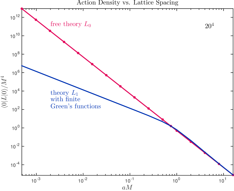
Figure 1: The dimensionless ground-state euclidian action density $\langle 0|L_{1}|0\rangle/M^{4}$ of the theory $L_{1}$ with finite Green’s functions (6, solid blue line) and that of the free theory $L_{0}$ (13, solid dotted red line) are plotted against the dimensionless lattice spacing $aM$ from $aM=2^{-11}$ to $aM=2^{4}$ for $m=M$. The two curves agree for $aM>2$, but as $aM\to 0$, the action density of the theory $L_{1}$ diverges quadratically as $4/(3a^{2})$ while that of the free theory $L_{0}$ diverges quarticly as $1/(2a^{4})$.

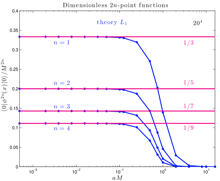
Figure 2: In the theory (6) with finite Green’s functions, the mean values $\langle 0|\phi^{2n}(x)|0\rangle/M^{2n}$ (solid dotted blue lines) approach the fractions $1/(2n+1)$ (solid red lines) as the dimensionless lattice spacing $aM\to 0$ as predicted Cahill (2013a).

I have run Monte Carlo simulations Creutz (1983); *Cahill14.4 with the action $S_{1}$ (12) and $S_{0}$ (14) on a $20^{4}$ lattice with periodic boundary conditions. In all the simulations of this paper, I allowed the fields to thermalize for a million sweeps and then took data in several runs of $2\times 10^{6}$ sweeps for each set of parameters. I restricted all the simulations to the equal-mass case, $m=M$, because my computer resources were limited.

Figure 1 plots the dimensionless ground-state action density $\langle 0|L_{1}|0\rangle/M^{4}$ of the theory $L_{1}$ with finite Green’s functions (6, solid blue line) and that $\langle 0|L_{0}|0\rangle/M^{4}$ of the free theory (13, solid dotted red line) against the dimensionless lattice spacing $aM$ from $aM=2^{-11}$ to $aM=2^{4}$ for $m=M$. The two curves agree for $aM>2$, but as $aM\to 0$, the action density of the theory $L_{1}$ diverges quadratically as $4/(3a^{2})$ while that of the free theory $L_{0}$ diverges quarticly as $1/(2a^{4})$. The theory $L_{1}$ is less singular than the free theory $L_{0}$.

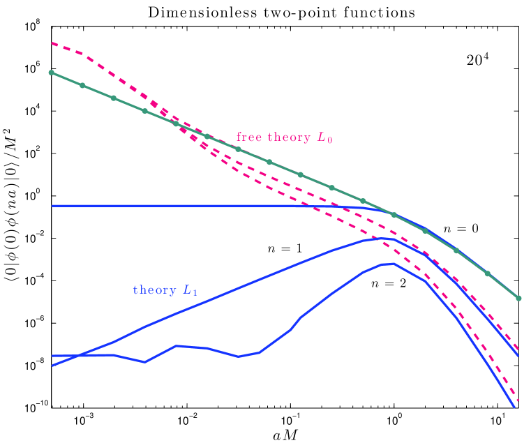
Figure 3: The dimensionless 2-point function $\langle 0|T\{\phi(x)\phi(x+na\hat{j})\}|0\rangle/M^{2}$ (16) of the theory $L_{1}$ with finite Green’s functions (6, solid blue lines) and of the free theory $L_{0}$ (13, dashed red lines), both on a $20^{4}$ lattice, are plotted for $n=0$, $n=1$, and $n=2$ against the dimensionless lattice spacing $am$ from $am=2^{-11}$ to $am=2^{4}$ for the case $m=M$. Also plotted (for $n=0$) is the exact 2-point function of the free theory $L_{0}$ (13) on an infinite lattice (18, solid dotted green line).

The lattice action density (12) vanishes in the limit $a\to 0$, unless $|\phi(x)|\geq M$, in which case it’s infinite. Thus, the field is limited to $|\phi(x)|<M$, and in the ratio (15) of path integrals that gives the mean value $\langle 0|\phi^{2n}(x)|0\rangle/M^{2n}$, the integrations over the field at $x^{\prime}\neq x$ all cancel. This mean value is therefore a ratio of one-dimensional integrals Cahill (2013a)

$$\langle 0|\phi^{2n}(x)|0\rangle=\frac{\bigintsss\!\phi^{2n}(x)\,e^{{}-S[\phi]}D\phi}{\bigintsss\!e^{{}-S[\phi]}D\phi}=\frac{\bigintsss_{-M}^{M}\!\phi^{2n}(x)\,d\phi(x)}{\bigintsss_{-M}^{M}\!d\phi(x)}=\frac{M^{2n}}{2n+1}.$$ (15)

The mean value of an odd power vanishes by symmetry. The lattice simulations for $m=M$ shown in Fig. 2 verify these formulas. The solid red horizontal lines are the fractions $1/(2n+1)$ for $n=1$, 2, 3, and 4; the lattice estimates of the dimensionless ground-state 2n-point functions $\langle 0|\phi^{2n}(x)|0\rangle/M^{2n}$ (solid dotted blue lines) rapidly converge to these lines as the dimensionless lattice spacing $aM$ falls below 1 and approaches 0.

In these simulations, the dimensionless 2-point function is the average of $N$ measurements of products of fields

$$\begin{split}\frac{1}{M^{2}}\,\langle 0|T\{\phi(x)\phi(x+na\hat{j})\}|0\rangle={}&\frac{1}{NM^{2}}\sum_{k=1}^{N}\,\phi_{k}(v)\,\phi_{k}(v+n\hat{j})\\ ={}&\frac{1}{N}\sum_{k=1}^{N}\,\varphi_{k}(v)\,\varphi_{k}(v+n\hat{j}).\end{split}$$ (16)

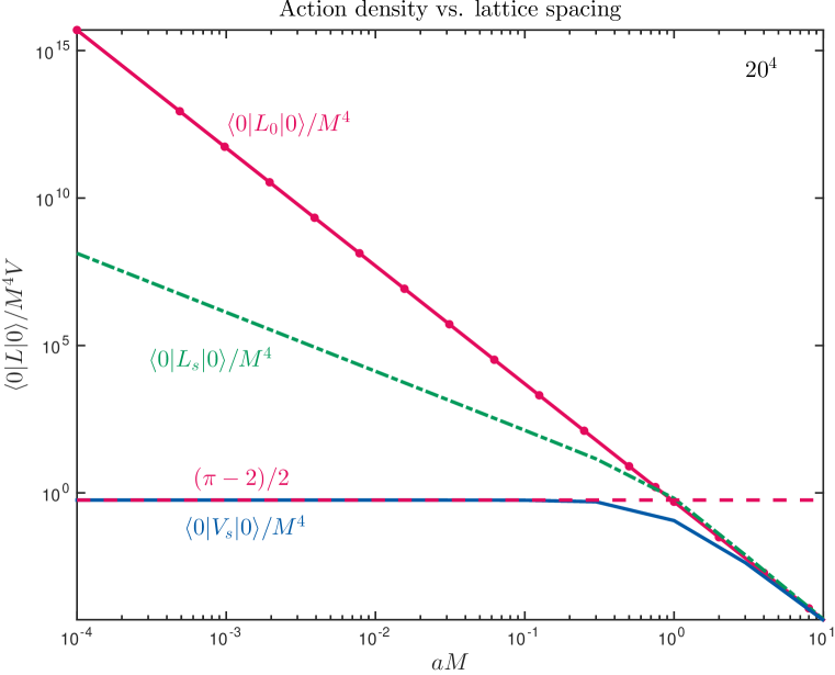
Figure 4: The dimensionless, ground-state action density $\langle 0|L_{s}|0\rangle/M^{4}$ (19, dot-dash green line) and potential-energy density $\langle 0|V_{s}|0\rangle/M^{4}$ of the theory $L_{s}$ (20, solid blue line) and that $\langle 0|L_{0}|0\rangle/M^{4}$ of the free theory [(13), solid dotted red line] are plotted against the dimensionless lattice spacing $aM$ from $aM=10^{-4}$ to $aM=10$ for $m=M$. As $aM\to 0$, the potential-energy density $\langle 0|V_{s}|0\rangle/M^{4}$ converges to the theoretical value $(\pi-2)/2$ [(20), dashed red line]. The action densities agree for $aM>2$, but as $aM\to 0$, the action density of the theory $L_{s}$ diverges quadratically as $4/(3a^{2})$ while that of the free theory $L_{0}$ diverges quarticly as $1/(2a^{4})$.

The exact dimensionless 2-point function of the free theory $L_{0}$ in the continuum is

$$\begin{split}\frac{1}{M^{2}}\,\langle 0|T\{\phi(x)\phi(x+na\hat{j})\}|0\rangle={}&\frac{1}{4\pi^{2}n^{2}a^{2}M^{2}}\,naM\,K_{1}(naM)\\ \approx{}&\frac{1-\frac{1}{4}\left(1-2\gamma+2\ln(2/naM)\right)(naM)^{2}}{4\pi^{2}n^{2}a^{2}M^{2}}\\ \approx{}&\frac{1}{(2\pi naM)^{3/2}}\,e^{-naM}\end{split}$$ (17)

in which the approximation of the second line holds for $naM<<1$ and that of the third for $naM>>1$. The exact dimensionless 2-point function of the free theory $L_{0}$ on an infinite lattice is

$$\begin{split}\frac{1}{M^{2}}\,\langle 0|T\{\phi(x)\phi(x+na\hat{j})\}|0\rangle={}&\frac{1}{a^{2}M^{2}}\int_{-\pi/a}^{\pi/a}\frac{a^{4}d^{4}q}{(2\pi)^{4}}\frac{\exp(inaq_{j})}{a^{2}M^{2}+2\sum_{k}(1-\cos aq_{k})}\\ ={}&\frac{1}{a^{2}M^{2}}\int_{-\pi/a}^{\pi/a}\frac{a^{4}d^{4}q}{(2\pi)^{4}}\frac{\exp(inaq_{j})}{a^{2}M^{2}+4\sum_{k}\sin^{2}(aq_{k}/2)}\\ ={}&\frac{1}{a^{2}M^{2}}\int_{-\pi}^{\pi}\frac{d^{4}p}{(2\pi)^{4}}\frac{\exp(inp_{j})}{a^{2}M^{2}+4\sum_{k}\sin^{2}(p_{k}/2)}\\ ={}&\frac{1}{\pi^{4}a^{2}M^{2}}\int_{0}^{\pi}\frac{\cos(np_{j})}{a^{2}M^{2}+4\sum_{k}\sin^{2}(p_{k}/2)}\,d^{4}p.\end{split}$$ (18)

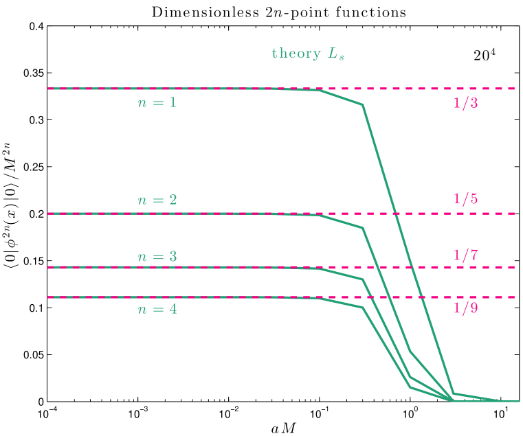
Figure 5: In the theory (19), which also has finite Green’s functions, the mean values $\langle 0|\phi^{2n}(x)|0\rangle/M^{2n}$ approach the fractions $1/(2n+1)$ as the dimensionless lattice spacing $aM\to 0$.

For fields separated by $n=0$, 1, and 2 lattice spacings on a $20^{4}$ lattice, Fig. 3 plots the dimensionless lattice 2-point function $\langle 0|T\{\phi(x)\phi(x+na\hat{j})\}|0\rangle/M^{2}$ (16) for the theory with finite Green’s functions [(6), solid blue lines] and for the free theory [(13), dashed red lines] against the dimensionless lattice spacing $aM$ from $aM=2^{-7}$ to $aM=2^{4}$ for the case $m=M$. The two theories agree for $aM\geq 2$. For separations of $n=0$ lattice spacings, Fig. 3 also plots the exact dimensionless 2-point function of the free theory $L_{0}$ (13) on an infinite lattice [(18), solid dotted green line] which reveals lattice artifacts for $aM\leq 2^{{}-5}$. For $aM<0.03$, the wobble in $\langle 0|T\{\phi(x)\phi(x+2a\hat{j})\}|0\rangle/M^{2}$ of the theory $L_{1}$ is due to insufficient statistics.

We turn now to the theory (7) with euclidian action density

$$L_{s}=\frac{1}{2}\,(\partial_{\mu}\phi(x))^{2}+m^{2}M^{2}\,\left(\frac{1}{\sqrt{1-\phi^{2}(x)/M^{2}}}-1\right)\equiv\frac{1}{2}\,(\partial_{\mu}\phi(x))^{2}+V_{s}(x).$$ (19)

This theory also has finite Green’s functions. Arguments similar to the ones that gave us the mean-value formulas (15) show that the mean value the potential-energy density $V_{s}$ in the ground state is

$$\langle 0|V_{s}(x)|0\rangle=(2M)^{-1}m^{2}M^{2}\int_{-M}^{M}\left(\frac{1}{\sqrt{1-\phi^{2}(x)/M^{2}}}-1\right)\,d\phi(x)\\ =\frac{1}{2}(\pi-2)\,m^{2}M^{2},$$ (20)

that the mean value of the $2n$th power of the field at a given point $x$ is

$$\langle 0|\phi^{2n}(x)|0\rangle=\frac{M^{2n}}{2n+1},$$ (21)

while those of the odd powers vanish by symmetry, and that the dimensionless action density in the ground state $\langle 0|L_{s}|0\rangle/M^{4}$ diverges as $4/(3a^{2})$. These predictions are verified for $m=M$ by the lattice simulations displayed in Figs. 4, 5, and 6. The dimensionless 2-point function $\langle 0|T\{\phi(x)\phi(x+na\hat{j})\}|0\rangle/M^{2}$ (16) of the theory $L_{s}$ with finite Green’s functions [(19), solid blue lines] and of the free theory $L_{0}$ [(13), dashed red lines], both on a $20^{4}$ lattice, are plotted in Fig. 6 for $n=0$, $n=1$, and $n=2$ against the dimensionless lattice spacing $am$ from $am=2^{-11}$ to $am=2^{4}$ for the case $m=M$. Also plotted (for $n=1$) is the exact 2-point function of the free theory $L_{0}$ (13) on an infinite lattice [(18), solid dotted green line].

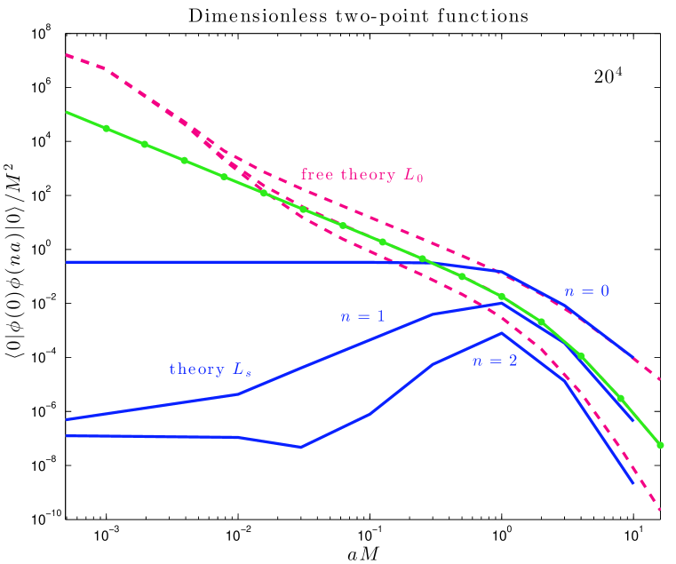
Figure 6: The dimensionless 2-point function $\langle 0|T\{\phi(x)\phi(x+na\hat{j})\}|0\rangle/M^{2}$ (16) of the theory $L_{s}$ with finite Green’s functions [(19), solid blue lines] and of the free theory $L_{0}$ [(13), dashed red lines], both on a $20^{4}$ lattice, are plotted for $n=0$, $n=1$, and $n=2$ against the dimensionless lattice spacing $am$ from $am=2^{-11}$ to $am=2^{4}$ for the case $m=M$. Also plotted (for $n=1$) is the exact 2-point function of the free theory $L_{0}$ (13) on an infinite lattice [(18), solid dotted green line].

III Theories with finite ground-state action densities

The euclidian action densities of the theories $L_{1}$ and $L_{s}$ (6 and 7) diverge because their derivatives contribute only quadratically to their action densities. We can make the mean value of the ground-state euclidian action density finite by using as the euclidian action density (10)

$$L_{f}=M^{4}\,\left(\frac{1}{\sqrt{1-M^{-4}\left[(\partial_{\mu}\phi(x))^{2}+m^{2}\phi^{2}(x)\right]}}-1\right)$$ (22)

or

$$L_{f,s}=M^{4}\left(\frac{1}{\sqrt{1-\partial_{\mu}\phi^{2}/M^{4}}}-1\right)+m^{2}M^{2}\left(\frac{1}{\sqrt{1-\phi^{2}/M^{2}}}-1\right).$$ (23)

The euclidian action on a lattice of spacing $a$ of the theory (22) is a sum over all $N^{4}$ vertices $v$ of the vertex action

$$\begin{split}S_{f}(v)={}&a^{4}M^{4}\left\{1-M^{-4}\left[\frac{1}{2}\sum_{j=1}^{4}\left(\frac{\phi(v)-\phi(v\pm\hat{j})}{a}\right)^{2}+m^{2}\phi^{2}(v)\right]\right\}^{-1/2}-a^{4}M^{4}\\ ={}&a^{4}M^{4}\left\{1-\left[\frac{1}{2}\sum_{j=1}^{4}\left(\frac{\varphi(v)-\varphi(v\pm\hat{j})}{aM}\right)^{2}+\frac{m^{2}}{M^{2}}\varphi^{2}(v)\right]\right\}^{-1/2}-a^{4}M^{4}\end{split}$$ (24)

in which the field $\varphi=\phi/M$ and the product $aM$ are dimensionless. The $\pm$ signs mean that we average the forward and backward derivatives.

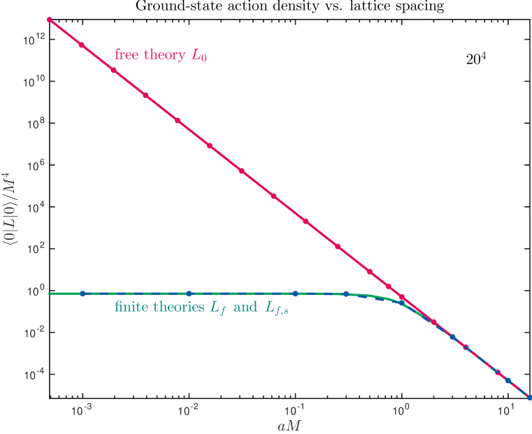
Figure 7: The ground-state dimensionless action densities $\langle 0|L_{f}|0\rangle/M^{4}$ and $\langle 0|L_{f,s}|0\rangle/M^{4}$ of the finite theories [(10), solid green line] and [(23), dashed-and-dotted blue line] and of the free theory $\langle 0|L_{0}|0\rangle/M^{4}$ [(13)–(14), solid dotted red line] on a $20^{4}$ lattice are plotted against the dimensionless lattice spacing $aM$ for $m=M$. As $aM\to 0$, the action densities of the finite theories approach $0.7120\,M^{4}$, while that of the free theory $L_{0}$ diverges quarticly as $1/(2a^{4})$.

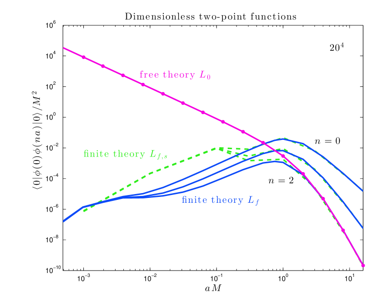
Figure 8: The dimensionless 2-point functions $\langle 0|T\{\phi(x)\phi(x+na\hat{j})\}|0\rangle/M^{2}$ (16) of the finite theories $L_{f}$ [(10), solid blue lines] and $L_{f,s}$ [(23), dashed green lines] on a $20^{4}$ lattice are plotted for $n=0$, $n=1$, and $n=2$ against the dimensionless lattice spacing $aM$ from $aM=2^{-11}$ to $aM=2^{4}$ for the case $m=M$. Also plotted (for $n=2$) is the exact 2-point function of the free theory $L_{0}$ (13) on an infinite lattice [(18), solid dotted red line].

We recover functional integrals like

$$\langle 0|L_{f}|0\rangle=\frac{\displaystyle{\int}L_{f}\,\exp\left[-\int\!L_{f}(\phi)\,d^{4}x\right]D\phi}{\displaystyle{\int}\exp\left[-\int\!L_{f}(\phi)\,d^{4}x\right]D\phi}.$$ (25)

by taking the twin limits $a\to 0$ and $N\to\infty$.

I have run Monte Carlo simulations with the lattice action (24) of the finite theory $L_{f}$ and with the lattice action of the closely related theory $L_{f,s}$ (23) on a $20^{4}$ lattice with periodic boundary conditions for the equal-mass case, $m=M$. Figure 7 plots the mean values (25) in the ground state of the dimensionless action densities $\langle 0|L_{f}|0\rangle/M^{4}$ [(10), solid green line] and $\langle 0|L_{f,s}|0\rangle/M^{4}$ (dashed-and-dotted blue line) as well as that of the free theory $L_{0}$ [(13), solid dotted red line] for values of the lattice spacing running from $a=2^{-11}/M$ to $a=2^{4}/M$. The three curves agree for $a>2/M$. But as $aM\to 0$, the action densities $\langle 0|L_{f}|0\rangle$ and $\langle 0|L_{f,s}|0\rangle$ approach $0.7120\,M^{4}$, while $\langle 0|L_{0}|0\rangle$ diverges quarticly as $1/(2a^{4})$. Incidentally, the ground-state action density $0.7120\,M^{4}$ of $L_{f}$ and $L_{f,s}$ would fit the experimental value $(0.00224\,\,\mbox{eV})^{4}$ of the dark-energy density Ade and others (Planck Collaboration); *Cahillpop-ph13 if we set $m=M=2.44$ meV.

For fields separated by $n=0$, 1, and 2 lattice spacings on a $20^{4}$ lattice, Fig. 8 plots the dimensionless lattice 2-point function $\langle 0|T\{\phi(x)\phi(x+na\hat{j})\}|0\rangle/M^{2}$ (16) for the finite theory $L_{f}$ [(10), solid blue lines] and for the similar theory $L_{f,s}$ [(23), dashed green lines] against the dimensionless lattice spacing $aM$ from $aM=2^{-11}$ to $aM=2^{4}$ for the case $m=M$. The two theories agree with each other and with the free theory $L_{0}$ for $aM\geq 1$, but as the dimensionless lattice spacing $aM\to 0$, the (bare) Green’s functions of $L_{f}$ and $L_{f,s}$ approach zero. Figure 8 also plots for separations of $n=2$ lattice spacings the exact dimensionless 2-point function of the free theory $L_{0}$ (13) on an infinite lattice [(18), solid dotted red line].

IV Masses

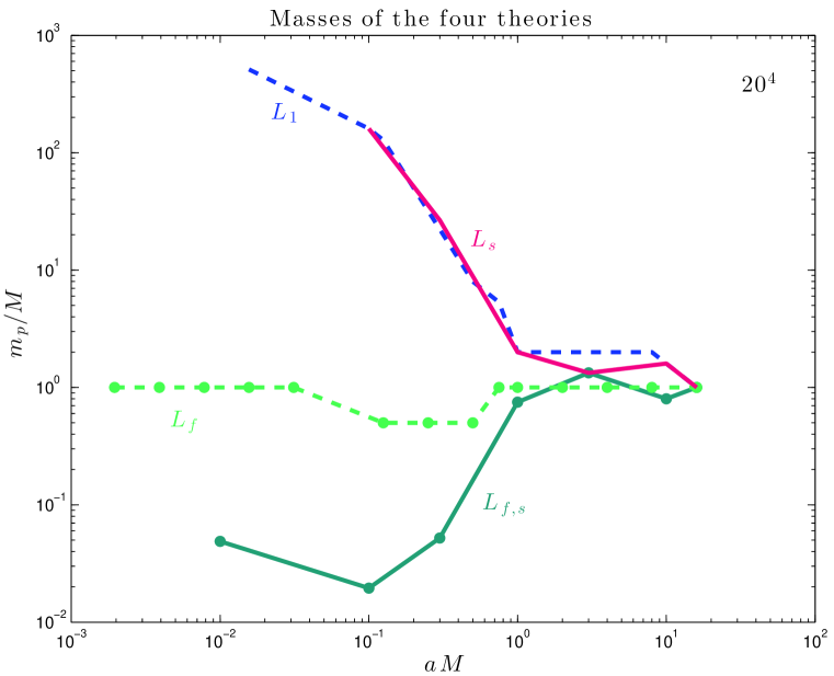
Figure 9: At various values of the dimensionless lattice spacing $aM$, the ratio of the physical mass $m_{p}$ (34) to the mass parameter $M$ is plotted for the theories $L_{1}$ [(6), dashed blue line], $L_{s}$ [(19), solid red line], $L_{f}$ [(10), dashed-and-dotted green line], and $L_{f,s}$ [(23), solid dotted blue-green line] for the case $m=M$ .

One may use analytic and lattice methods to estimate the physical masses of the bosons of the four theories described in sections II and  LABEL:Theories_with_finite_ground-state_energies.

Although the theories $L_{1}$ and $L_{s}$ have finite Green’s functions, they describe bosons of infinite mass. We can see why the mass of the theory $L_{1}$ diverges by considering the equation of motion of its field $\phi(x)$ in Minkowski spacetime

$$\ddot{\phi}(x)-\triangle\phi(x)=-m^{2}\phi(x)\left[1-\phi^{2}(x)/M^{2}\right]^{-2}.$$ (26)

I will approximate the nonlinear term $(1-\phi^{2}/M^{2})^{-2}$ by its mean value in the vacuum

$$\ddot{\phi}(x)-\triangle\phi(x)=-m^{2}\phi(x)\,\langle 0|\left[1-\phi^{2}(x)/M^{2}\right]^{-2}|0\rangle.$$ (27)

An argument similar to the one that gave us the mean-value formulas (15) shows that this mean value diverges

$$\begin{split}\langle 0|\left[1-\phi^{2}(x)/M^{2}\right]^{-2}|0\rangle={}&(2M)^{-1}\int_{-M}^{M}\left[1-\phi^{2}/M^{2}\right]^{-2}\,d\phi\\ ={}&(2M)^{-1}\int_{-M}^{M}\frac{1}{(1-\phi/M)^{2}(1+\phi/M)^{2}}\,d\phi=\infty.\end{split}$$ (28)

So the physical mass of the boson is infinite.

Similarly, the equation of motion of the field of the second theory $L_{s}$ in Minkowski space is

$$\ddot{\phi}(x)-\triangle\phi(x)=-m^{2}\phi(x)\left[1-\phi^{2}(x)/M^{2}\right]^{-3/2}.$$ (29)

I again use the approximation

$$\ddot{\phi}(x)-\triangle\phi(x)=-m^{2}\phi(x)\,\langle 0|\left[1-\phi^{2}(x)/M^{2}\right]^{-3/2}|0\rangle.$$ (30)

The mean value is infinite

$$\begin{split}\langle 0|\left[1-\phi^{2}(x)/M^{2}\right]^{-3/2}|0\rangle={}&(2M)^{-1}\int_{-M}^{M}\left[1-\phi^{2}/M^{2}\right]^{-3/2}\,d\phi=\infty,\end{split}$$ (31)

and so is the mass of the boson. Figure 9 verifies these estimates of the masses bosons of theories $L_{1}$ and $L_{s}$.

The theories $L_{f}$ and $L_{f,s}$ are much more complicated than $L_{1}$ and $L_{s}$, and I don’t have a good analytic argument that shows that their masses are finite. But these theories bound the derivatives $(\partial_{\mu}\phi)^{2}$ as well as the fields $\phi^{2}$, and the lattice action (24) shows that if the derivatives are to be bounded in the limit $aM\to 0$, then the mean values of the fields $\langle 0|\phi^{2n}(x)|0\rangle$ must become tiny in that limit as a glance at Fig. 8 reveals. Thus, we expect the masses of the bosons of the second pair of theories $L_{f}$ and $L_{f,s}$ to be finite.

I used the 2-point functions displayed in Figs. 3, 6, and 8 to estimate the masses of the bosons of the four theories as follows. Let

$$f(naM)\equiv\frac{\langle 0|T\{\phi(x)\,\phi(x+na\hat{j})\}|0\rangle}{M^{2}}$$ (32)

be the dimensionless 2-point function for one of the four theories simulated on a $20^{4}$ lattice, and let $f_{0}(naM)$ be the same thing for the free theory $L_{0}$. For each theory, and each value of the dimensionless lattice spacing $aM$, I minimized the sum

$$\sum_{n=0}^{1}\left(\frac{f((n+1)aM)}{f(naM)}-\frac{f_{0}((n+1)(aM)^{\prime})}{f_{0}(n(aM)^{\prime})}\right)^{2}$$ (33)

over values of $(aM)^{\prime}$ from $(aM)^{\prime}=2^{-11}$ to $(aM)^{\prime}=2^{4}$ at which I had measured the 2-point function of the free theory on a $20^{4}$ lattice. I took the upper limit on the sum over $n$ to be unity rather than 2 or more in order to stay within a range in which my statistical errors were small. I then estimated the physical mass of the boson to be the limit

$$\lim_{aM\to 0}m(aM)\equiv\left(\lim_{aM\to 0}\frac{(aM)^{\prime}}{aM}\right)\,M.$$ (34)

The values of the mass ratios from my simulations of the four theories are displayed in Fig. 9. This figure shows that the masses of the bosons of the first two theories $L_{1}$ and $L_{s}$ diverge as $aM\to 0$, but that those of the bosons of the third and fourth theories are finite with $m_{f}\approx M$ and $m_{f,s}\approx M/20$.

V Speculations about confinement, gravity, and fermions

Many nonrenormalizable theories are less singular than that of a free field. The space of such theories is vast. We can make a typical theory of scalar and vector bosons less singular by replacing its euclidian action density $L$ by Cahill (2013d)

$$L^{\prime}=\frac{L}{1-L/M^{4}}\qquad\mbox{or by}\qquad L^{\prime\prime}=M^{4}\left[\exp(L/M^{4})-1\right]$$ (35)

or by any expression that grows dramatically for large $L$.

V.1 Confinement

The euclidian action density of $SU(3)$ gauge theory (without fermions and $\theta$-vacua) is the trace

$$L_{3}=\frac{1}{2g^{2}}\,{\rm Tr}\left(F^{2}_{\mu\nu}\right)$$ (36)

in which the Faraday matrix is $F_{\mu\nu}=g\,t^{a}\,F^{a}_{\mu\nu}$, the generators $t^{a}$ of $SU(3)$ are half the Gell-Mann matrices, and $F^{a}_{\mu\nu}=\partial_{\mu}A^{a}_{\nu}-\partial_{\nu}A^{a}_{\mu}-gf_{abc}A^{b}_{\mu}A^{c}_{\nu}$. The theory described by

$$L^{\prime}_{3}=m^{4}\left(\frac{1}{\sqrt{1-L_{3}/m^{4}}}-1\right)\quad\mbox{or by}\quad L^{\prime\prime}_{4}=M^{4}\left(e^{L_{3}/M^{4}}-1\right)$$ (37)

has Green’s functions that are less singular than those of the $L_{3}$ theory (36).

To simulate such a theory on a lattice while preserving gauge invariance, one may represent the matrix elements $A_{\mu\>bc}$ of the gauge field matrix $A_{\mu}=i\,t^{a}A_{\mu}^{a}$ in terms of three orthonormal vectors, $e^{\dagger}_{b}\cdot e_{c}=\delta_{bc}$, as inner products of a vector $e^{\dagger}_{b}$ with the derivative $\partial_{\mu}e_{c}$ of another vector Narasimhan and Ramanan (1961); *Ramanan1963; *Cahill11.51

$$A_{\mu\>bc}=i\,t^{a}_{bc}A_{\mu}^{a}=e^{\dagger}_{b}\cdot e_{c,\mu}\equiv e^{\dagger}_{b}\cdot\partial_{\mu}e_{c}.$$ (38)

In this notation, in which commas denote derivatives, the elements $F_{\mu\nu\>ab}$ of the Faraday matrix are

$$F_{\mu\nu\>ab}=\bm{[}D_{\mu},D_{\nu}\bm{]}_{ab}=e^{\dagger}_{a,\mu}\cdot e_{b,\nu}-e^{\dagger}_{a,\mu}\cdot e_{c}\,\,e^{\dagger}_{c}\cdot e_{b,\nu}-e^{\dagger}_{a,\nu}\cdot e_{b,\mu}+e^{\dagger}_{a,\nu}\cdot e_{c}\,\,e^{\dagger}_{c}\cdot e_{b,\mu}.$$ (39)

This matrix vanishes unless the vectors have $n>3$ components.

Wilson Wilson (1974), Creutz Creutz (1979); *PhysRevLett.45.313, and others have demonstrated quark confinement on the lattice by replacing the euclidian action of pure continuum QCD

$$S_{QCD}=\frac{1}{2g^{2}}\int{\rm Tr}\left(F^{2}_{\mu\nu}\right)\,d^{4}x=\int L_{3}\,d^{4}x$$ (40)

by a sum over the plaquettes $\Box$ of a lattice

$$S_{W}=\sum_{\Box}S_{\Box}$$ (41)

of Wilson’s action $S_{\Box}$ which is the trace of the product of elements $U$ of $SU(3)$ on the links that form the plaquette

$$S_{\Box}=\beta\,\left[1-(1/3)\mathrm{Re}\,{\rm Tr}\left(U_{ij}U_{jk}U_{k\ell}U_{\ell i}\right)\right].$$ (42)

Yet there is a big difference between the continuum action density ${\rm Tr}(F^{2}_{\mu\nu})/2g^{2}$ which can be arbitrarily large and Wilson’s action $S_{\Box}$ which is bounded by $\beta$. This gap is bridged if one uses the action density $L^{\prime}_{3}$ which keeps ${\rm Tr}(F^{2}_{\mu\nu})/2g^{2}$ bounded like Wilson’s $S_{\Box}$. The action density $L^{\prime\prime}_{3}$ has a similar effect. Simulations guided by $L^{\prime}_{3}$ or $L^{\prime\prime}_{3}$ may exhibit ground-state mean values of the squares of the gauge fields that are tiny enough to justify Wilson’s compactification of the gauge fields. Thus, the ideas of this subsection may make possible a demonstration of quark confinement without the need to assume that compactification is justified.

V.2 Gravity

The euclidian action density of general relativity is not bounded below, and so the recipes (35) don’t work for it. Instead, we can use, for instance,

$$L^{\prime}_{E}=\frac{1}{16\pi\alpha G^{2}_{N}}\left[\cosh^{2}\theta\left(\frac{1}{(1-G_{N}\,R_{e})^{\alpha}}-1\right)+\sinh^{2}\theta\left(\frac{1}{(1+G_{N}\,R_{e})^{\alpha}}-1\right)\right]\sqrt{|g|}$$ (43)

in which $\alpha>0$, $R_{e}$ is the euclidian Ricci scalar, and $|g|$ is the absolute value of the determinant of the euclidian metric tensor. We also could use

$$L^{\prime\prime}_{E}=\frac{1}{16\pi G^{2}_{N}}\left[\cosh^{2}\theta\left(e^{G_{N}R_{e}}-1\right)+\sinh^{2}\theta\left(e^{-G_{N}R_{e}}-1\right)\right]\sqrt{|g|}.$$ (44)

The resulting theories are less singular than conventional quantum gravity.

V.3 Fermions

The energy density of the ground state of a free Fermi field is negative and quarticly divergent, while that of its excited states can be arbitrarily high. So it may make sense to use a construction similar to (43 ) and (44). Instead of the usual fermionic action density

$$L_{F}=\bar{\psi}(x)(\gamma_{\mu}D_{\mu}+m)\psi(x),$$ (45)

one could use

$$L^{\prime}_{F}=\frac{M^{4}}{\alpha}\left[\cosh^{2}\theta\left(\frac{1}{(1-L_{F}/M^{4})^{\alpha}}-1\right)+\sinh^{2}\theta\left(\frac{1}{(1+L_{F}/M^{4})^{\alpha}}-1\right)\right]$$ (46)

in which $\alpha>0$ or

$$L^{\prime\prime}_{F}=M^{4}\left[\cosh^{2}\theta\left(e^{L_{F}/M^{4}}-1\right)+\sinh^{2}\theta\left(e^{-L_{F}/M^{4}}-1\right)\right].$$ (47)

These theories are less singular than the usual theories of fermions.

VI Summary

Some nonrenormalizable theories are less singular than every renormalizable theory. The space of such less-singular nonrenormalizable theories is vast. Whether any of them is realistic or true is unknown. Two of them, $L_{1}$ (6) and $L_{s}$ (19), discussed in section II, have finite Green’s functions and quadratically divergent ground-state action densities and describe infinitely massive particles. Two others, $L_{f}$ (10) and $L_{f,s}$ (23) of section III, have finite ground-state action densities and describe particles of finite mass. Their bare Green’s functions are finite and vanish in the continuum limit. Section IV is about how I estimated the masses of the particles of these four theories. Section V suggests ways of extending the present work to theories of gauge fields, gravity, and fermions. Each theory of this paper reduces to its renormalizable counterpart in the appropriate limit; for the theories $L_{1}$, $L_{s}$, $L_{f}$, and $L_{f,s}$, that limit is $M\to\infty$. The ways of coping with infinities outlined above apply to theories in any number of space-time dimensions.