We demonstrate using the classical density functional theory (DFT) model that an intermediate degree of mass localization in the amorphous state is essential for producing the boson peak. The localization length $\ell$ is identified from the width of the gaussian density profile in terms of which the inhomogeneous density $n({\bf x})$ of the solid is expressed in DFT. At a fixed average density, there exists a limiting value $\ell_{0}$ of $\ell$ signifying a minimum mass localization in the amorphous state. For more delocalized states ($\ell>\ell_{0}$) occurrence of boson peak is unfeasible .

Localization, disorder and boson peak in an amorphous solid

Studies of inelastic scattering of light and neutron from amorphous solids show that the disordered systems are characterized by an excess density of vibrational modes over that predicted by the standard Debye distribution. This excess in the density of states (DOS) $g(\omega)$ for a disordered system typically occurs at the THz frequency ($\omega$) range and is identified as the so called boson peak in the $g(\omega)/\omega^{2}$ vs. $\omega$ plot. The boson peak height decreases and its location shifts towards the higher frequencies with the increase of pressure or density zeller -AM . A number of different theoretical models have been developed to explain the anomalous low-energy excitations schober -dove . It is now generally believed that the boson peak is a manifestation of disorder and is key to the understanding of the vibrational states of glassy materials. The origin of boson peak in the disordered solid has been often linked to transverse sound modes for the systemspd_bpk . It has been argued that the boson peak results from a band of random transverse acoustic vibrational states schirmacher . Extensive computer simulations of several glass forming systems tanaka also indicated subsequently that the origin of the boson peak is the transverse vibrational modes associated with defective soft structures in the disordered state. In a recent work, Chumakov et al. chumakov explain the boson peak in terms of (predominantly) transverse sound waves.

A common aspect of a class of the boson peak models mentioned above is that they are based on the existence of localized modes in the amorphous solid zorn . Longitudinal acoustic phonon modes are observed in a liquid by ultrasonic, optical, or inelastic scattering experiments. These hydrodynamic modes occur due to the conservation laws for the system. For the crystalline state the isotropic symmetry of the liquid is broken and the constituent particles vibrate around the sites of a lattice with long range order. This symmetry breaking leads to the development of the Goldstone modes goldstone or the transverse sound modes in the crystal in addition to the longitudinal sound modes. For the amorphous solid the symmetry is not broken over long length scales like that in a crystal. When the atomic vibration wavelength in a liquid approaches the atomic nearest neighbor distance, i.e., in the tera hertz frequency region, there is a solid like cage formation giving rise to a restoring force for the acoustic transverse modes.

A typical choice of the order parameter for the crystalline as well as the amorphous state is the inhomogeneous density $n({\bf r})$ with smooth spatial dependence. The density for the solid state is expressed in terms of gaussian profiles of width $\ell$ and centered on the sites of a chosen lattice $\{{\bf R}_{i}\}$ PT .

$$n({\bf r})={\left(\frac{\alpha}{\pi}\right)}^{\frac{3}{2}}\sum_{{\bf R}_{i}}e^{-\alpha{({\bf r}-{\bf R_{i}})}^{2}},$$ (1)

with $1/\sqrt{\alpha}=\ell$. The coarse grained picture for the solid presented above involves two inherent length scales. First, the microscopic length scale $\sigma$ (say) associated with the interaction potential between the constituent particles. For a hard sphere potential, $\sigma$ corresponds to the hard sphere diameter. Second, the length $\ell$ which represents the degree of localization of mass in the system. The homogeneous liquid state is characterized by the limit $\alpha{\sigma^{2}}\rightarrow{0}$ or $\ell>>\sigma$. The sharply localized density profiles of the crystalline state correspond to the limit $\alpha\sigma^{2}>>1$ or $\ell<<\sigma$. The ratio $\ell/\sigma$ is generally referred to as the Lindeman parameter for the crystalline. In the present work we compare the free energy contribution due to the vibrational modes in the amorphous state to the corresponding density functional result for the ideal gas part $f_{\mathrm{id}}[n]$spd_book of the free energy for an inhomogeneous density $n({\bf r})$. We show that for a a chosen average density, the characteristic gaussian profile of $n({\bf r})$ signifies a minimum localization length $\ell_{0}$ below which the appearance of boson peak in the reduced density of states is unfeasible.

The equilibrium state of the fluid is identified by minimizing a proper thermodynamic potential or free energy with respect to the density $n({\bf x})$. The free energy is expressed as a sum of two parts which are respectively the free energy of the non-interacting system $F_{\mathrm{id}}$ and the contribution $F_{\mathrm{ex}}$ due to interactions between the particles. $F_{\mathrm{id}}$ is obtained from the logarithm of the partition function ${(V/\wedge^{3})}^{N}/N!$ for the noninteracting system of $N$ particle, where $\wedge=\hbar/\sqrt{2\pi{m}k_{B}T}$ denotes the thermal wave length at temperature $T$. Thus ${\beta}F_{\mathrm{id}}=Vn_{0}(\ln({n_{0}}\wedge^{3})-1)$ for the uniform density fluid $n_{0}$. For the inhomogeneous density $n({\bf x})$, the expression for the free energy is easily generalized to $\beta{F}_{\mathrm{id}}[n]=\int d{\bf r}n({\bf r})[\ln\{n({\bf r})\wedge^{3}\}-1]$. For the uniform density $n_{0}$ changing to a nonuniform one $n({\bf x})$, the ideal gas contribution for the $N$ particles system changes by an amount $n_{0}\int d{\bf r}\tilde{n}({\bf r})[\ln\tilde{n}({\bf r})]$, where $\tilde{n}({\bf r})=n({\bf r})/n_{0}$. Since by definition $\tilde{n}({\bf r})$ is always positive, using the Gibbs inequality $\{x\ln{x}-x+1\}\geq 0$ for positive $x$, it follows that entropy drops upon localization of the particles. This is a result of the restriction of available phase space. If $\alpha$ is larger than a limiting value $\alpha_{0}$ (say) the density $n({\bf r})$ is well approximated in terms of the gaussian profile centered at the nearest lattice site. The free energy per particle $f_{\mathrm{id}}$ for large $\alpha\sigma^{2}$ is obtained as,

$$f_{\mathrm{id}}[\alpha]\approx-\frac{5}{2}+3\ln\left(\sqrt{\frac{\alpha}{\pi}}\wedge\right).$$ (2)

In a microscopic approach, vibrational modes with localized density profiles contribute to the free energy and the latter is obtained in terms of the density of vibrational states $g(\omega)$ of the system. The free energy of the non-interacting system is obtained as $F_{\mathrm{id}}=-k_{B}T\ln Z_{N}~{}$ where $Z_{N}$ is the partition function for 3N harmonic oscillators in constant NVT ensemble. Going from discrete to continuum in the frequency spectrum, we obtain the ideal gas free energy per particle in units of $\beta^{-1}$ as ${\beta}F_{\mathrm{id}}/N=\int_{0}^{1}\kappa(x_{m}x)\bar{g}(x)dx~{}~{}\equiv f_{0}[\bar{g},x_{m}(\alpha)]$, where $\kappa(x)=-\frac{1}{4}\{x+\ln[1-e^{-x}]-2x/(e^{x}-1)\}$. $\omega_{m}$ is the upper cutoff of frequency up to which $g(\omega)$ is nonzero and it is expressed in terms of the dimensionless quantity $\beta\hbar{\omega}_{m}=x_{m}{\equiv}x_{m}(\alpha)$. The scaled density of states $\bar{g}(x)$ is obtained from $g(\omega)$ as $\bar{g}(x)={(3n_{0})}^{-1}\omega_{m}g(\omega)$ where $x=\omega/\omega_{m}$ is the reduced frequency. The expression for $\kappa(x)$ indicates the functional dependence of the integral $f_{0}$ on the scaled density of states $\bar{g}$. There are $3n_{0}$ vibrational modes for an average $n_{0}$ number of particles in a unit volume giving rise to the normalization condition $\int_{0}^{\omega_{m}}g(\omega){d\omega}=3n_{0}$ for $g(\omega)$. The cutoff frequency $\omega_{m}$ is a characteristic property of the material and sets the shortest length scale for the vibrational modes. For the Debye distribution, $g(\omega)=g_{D}(\omega)\equiv(9n_{0}/\omega_{D}^{3})\omega^{2}$ is nonzero in the range $0\leq{\omega}\leq{\omega}_{D}$. The Debye frequency $\omega_{D}$ is obtained as $\omega_{D}={(6\pi{n_{0}})}^{1/3}c$, with $c$ being the speed of sound. The scaled (Debye) distribution $\bar{g}_{D}$ as $\bar{g}_{D}(x)=3x^{2}$ where $x=\omega/\omega_{D}$. Considering the case $x_{m}{\equiv}x_{D}=\beta\hbar\omega_{D}<<1$, analysis of the integral $f_{0}[\bar{g},x_{m}(\alpha)]$ for $\bar{g}(x)\equiv{\bar{g}_{D}(x)}$ obtains the following result to leading orders in $x_{D}$:

$$f_{0}[\bar{g}_{D},x_{D}]=-\frac{5}{2}+3\ln x_{D}+O(x_{D}^{2}).$$ (3)

This mapping identifies the Debye cutoff frequency $\omega_{D}$ in terms of the corresponding width parameter $\alpha$ of density functional description as $\beta\hbar\omega_{D}{\equiv}x_{D}(\alpha)=\sqrt{{\alpha}/{\pi}}\wedge$. For a given $\wedge$, a corresponding $\alpha_{0}$ is identified such that for all $\alpha\geq{\alpha}_{0}$ the asymptotic form (2) will represent the ideal gas free energy. The value of $\wedge/\sigma$ should be such that $x_{D}(\alpha_{0})\leq{x_{L}}$ where the asymptotic form (3) for $f_{0}(x)$ holds for $x<{x_{L}}$.

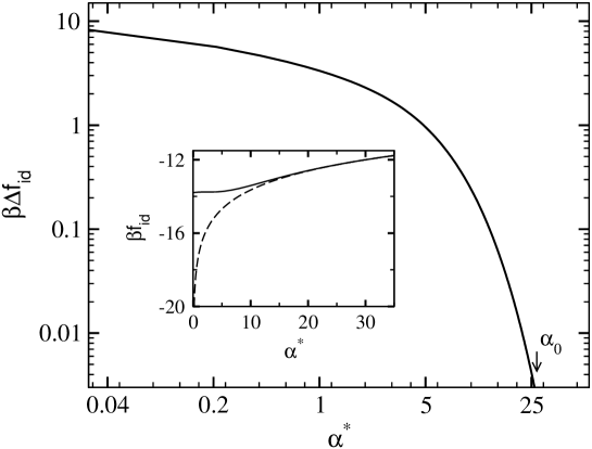
Figure 1: Inset : ideal gas part of free energy $f_{\mathrm{id}}$ per particle from numerical evaluation of the density functional expression (solid line) and from the asymptotic formula (2) (dashed line). The difference between the the asymptotic formula and the numerical result for $f_{\mathrm{id}}$ is shown in an enlarged form in the main figure for the $0<\alpha<\alpha_{0}$ region.

In DFT the free energy $f_{\mathrm{id}}(\alpha)$ for the amorphous state is evaluated numerically using the $n({\bf r})$ corresponding to the parameter value $\alpha$. The centers for the gaussian density profiles $\{{\bf R}_{i}\}$ are distributed on a random lattice and the corresponding site-site correlation function $g(R)$ is obtained from the Bernal’s Bernel random structure generated through the Bennett algorithm Benett . We approximate the $g(R)$ through the following relation $g(R)=g_{B}[R{(\eta/\eta_{0})}^{1/3}]$ where $\eta$ denotes the average packing fraction and $\eta_{0}$ is used as a scaling parameter for the structure lowen such that at $\eta=\eta_{0}$ Bernal’s structure is obtained. Smaller the parameter $\alpha$ in $n({\bf x})$, larger number of sites are needed to be included for an accurate evaluation of the $f_{\mathrm{id}}$. The free energy evaluated numerically agrees with the corresponding asymptotic expression (2) for $\alpha\geq\alpha_{0}$. This is shown in the inset of Fig. 1. The difference $\Delta{f}_{\mathrm{id}}$ between the two evaluations of $f_{\mathrm{id}}$ is shown in Fig. 1 for $\alpha<\alpha_{0}$ range. This result corresponds to hard sphere system with the fixed average density $n_{0}\sigma^{3}=1.1$ or packing fraction $\varphi=\pi{n_{0}}\sigma^{3}/6=.576$. The thermal wavelength is kept constant at $\wedge/\sigma=0.0137$. The free energy obtained from the DFT expression $f_{\mathrm{id}}[n({\bf r})]$ corresponding to $n({\bf r})$ in the range $\alpha<\alpha_{0}$, deviates completely from the asymptotic result (2). It extends to the correct $\alpha{\rightarrow}0$ limit $(\ln\{n_{0}\wedge^{3}\}-1)$ for the uniform liquid state. A key observation here is that the free energy curve for small $\alpha<\alpha_{0}$ matches with the corresponding result obtained from the microscopic expression $f_{0}[\bar{g},x_{m}(\alpha)]$ with a modified density of states which is different from the Debye distribution. The normalization condition for $g(\omega)$ is maintained with a corresponding $\omega_{m}(\alpha)$ or equivalently $x_{m}(\alpha)$ different from that for the Debye case ($=\sqrt{{\alpha}/{\pi}}\wedge$). Therefore we require that the function $x_{m}(\alpha)$ $\rightarrow$ $x_{D}(\alpha)$ as $\alpha\rightarrow{\alpha_{0}}$. The correction part in this functional relation is denoted by $C(\alpha)$, such that $x_{m}(\alpha)=x_{D}(\alpha_{0})+C(\alpha)$ with $C(\alpha){\rightarrow}0$ as $\alpha{\rightarrow}\alpha_{0}$. Similarly, for the scaled distribution function $\bar{g}(x)$ we use a correction over the corresponding Debye form $\bar{g}_{D}(x)=3x^{2}$ in terms of the function $\Delta$, such that $\bar{g}(x,x_{m}(\alpha))=3x^{2}(1+\Delta(x,\alpha))$. Since for all frequencies $x$, we must have $g\rightarrow{\bar{g}_{D}}$ as $\alpha{\rightarrow}\alpha_{0}$, we express $\Delta$ with the separation of variables. Thus $\Delta(x,\alpha)=B(\alpha)\tilde{\Delta}(x)$ where $B(\alpha){\rightarrow}0$ as $\alpha{\rightarrow}\alpha_{0}$. Furthermore in order to maintain the normalization condition of $g(\omega)$, the function $\tilde{\Delta}(x)$ for all $\alpha$ must satisfy $\int_{0}^{1}x^{2}\tilde{\Delta}(x)dx=0$. The two functions $C(\alpha)$ and $B(\alpha)$ are parameterized in terms of two respective polynomials of the separation parameter $\epsilon=1-\alpha/\alpha_{0}$. These functions are determined by requiring that the $f_{0}[\bar{g},x_{m}(\alpha)]$ obtained with the corresponding $\bar{g}$ and $x_{m}$ agree with that of the DFT expression for $f_{\mathrm{id}}$ in the range $\alpha{\leq}\alpha_{0}$. We choose the $x$ dependence of the $\tilde{\Delta}(x)$ so as to have an intermediate peak over the whole frequency range. The relative frequency $x$ at the peak of $\tilde{\Delta}(x)$ is a parameter which is kept fixed through out this work. In order to maintain the positivity of the density of states the function $\tilde{\Delta}(x)$ is also kept confined in the range $\pm{1}$. In Fig. 2 we show the results obtained for the appropriate density of states $\bar{g}(x)$ which satisfy the above constraints of density functional theory. The reduced density of states $g(\omega)/\omega^{2}$ vs. $\omega/\omega_{D}$ is shown in Fig. 2 for three different values of the localization parameter $\ell=1/\sqrt{\alpha}$. The height $h_{B}$ of the boson peak increases as $\ell$ grows and is shown in the inset of Fig. 2. Larger $\ell$ or smaller $\alpha$ corresponds to increased spreading of the density profiles and hence decreased localization.

As the density profiles get increasingly spread out, i.e., as $\alpha$ decreases, the intensity or height of the boson peak continues to grow while upper cutoff $\omega_{m}$ of the frequency keeps decreasing. However, this trend does not continue indefinitely towards $\alpha{\rightarrow}0$. To understand this behavior we note that the upper cutoff $\omega_{m}$ sets the shortest wavelength $\lambda_{\mathrm{min}}$ for the sound waves. In a valid continuum description of the solid, $\lambda_{\mathrm{min}}$ cannot get smaller than the average mean square displacement of the individual particles. In the density functional theory formulated in terms of gaussian density profiles, the average particle displacement is $\ell=1/\sqrt{\alpha}$ and this is a reasonable estimate for $\lambda_{\mathrm{min}}$. The corresponding upper limit in the frequency of the sound wave is obtained from the relation ${\Omega^{L}}/(2\pi{c})=\sqrt{\alpha}$ where $c$ is the speed of sound. In Fig. 3, for $n_{0}\sigma^{3}=1.1$ this limiting value for the upper limit vs. cutoff $\sqrt{\alpha}$ is shown as a dashed line. The corresponding upper cutoff of the frequency $\omega_{m}(\alpha)$ obtained by matching microscopic expression for the free energy with the density functional expression (as described with respect to Fig. 2) is shown as a solid line. We mark with an arrow in Fig. 3, the point $\alpha=\alpha_{\mathrm{min}}$ where the two lines cross. This point depicts the maximum delocalized state for which the boson peak in $g(\omega)$ is observed in the vibrational density of states. For more delocalized states the description in terms of sound waves breaks down. In the inset of Fig. 3, we show how the point of maximum delocalization obtained in the main figure changes with the density of a hard sphere system.

Metastable states of strongly heterogeneous density distribution has been obtained spd_kaur ; kim-munakata ; chandan-sood with free energy minimum intermediate between the uniform liquid and crystals with long range order. We regulate the parameter $\eta_{0}$ to define specific sets of random structures. The low $\alpha$ or partially delocalized state exists only if total free energy is computed with the $n({\bf x})$ for lattice points $\{{\bf R}_{i}\}$ on a random structure. Thus disorder is essential for locating the metastable minimum of the free energy in the delocalized region ($\alpha\leq{\alpha}_{0}$). This is due to the interaction contribution to the free energy. However the corresponding $F_{\mathrm{id}}$ in the small $\alpha$ region remains the same with $\{{\bf R}_{i}\}$ representing a regular crystalline lattice with long range order instead of the Bernel structure. With $m_{i}=\exp[-K_{i}^{2}/(4\alpha)]$ the definition (1) for the density $n({\bf r})$ reduces to the form $n({\bf r})=n_{0}+\sum_{i}m_{i}e^{i{\bf K}_{i}.{\bf r}}$ in terms of an expansionshenoxtoby involving reciprocal lattice vector (RLV) $\{{\bf K}_{i}\}$ . It is useful to note at this point that the boson peak in disordered system has been studied in terms of a geometrically perfect crystal having random interactions between the neighbors schirmacher ; Elliott .

For the hard sphere system with $n_{0}\sigma^{3}=1.1$ we obtain the interaction contribution to the free energy in terms of standard Ramakrishnan-Yussouff functional RY using the solution of the Percus-Yevick equation with Verlet-WeissHG . For the heterogeneous glassy state, the free energy barrier $f_{B}$ is obtained as the height of the maximum in the corresponding free energy curve from the metastable minimum at small nonzero $\alpha$ (inset (a) of Fig. 4). For the optimum value of $\alpha$ signifying a metastable state, $g(\omega)$ is obtained. In Fig. 4 we show the variation of $f_{B}$ for the parameter range $.62<\eta_{0}<.68$, with the corresponding boson peak height $h_{B}$. As the free energy barrier $f_{B}$ becoming weaker, the height of the boson peak $h_{B}$ goes down. In the inset (b) of Fig. 4 is shown the $f_{B}$ vs. $\ell=1/\sqrt{\alpha}$ curve. As the mass localization gets weaker, i.e. with decreasing(increasing) of $\alpha$($\ell$) the barrier height $f_{B}$ gets smaller. A lower barrier height implies that the structural degradation is less hindered in the corresponding system, i.e., represents a glassy material of higher fragility. The dependence of the peak height $h_{B}$ and the peak frequency $\omega_{p}$ on the pressure are respectively shown in Fig. 5 and its inset and conforms to experimental findings.

An important characteristic of the boson peak is that it gets weaker, more fragile the system is. This link between the long-time relaxation behavior (fragility) of the glass forming material and the vibrational modes in the THz region, follows in a natural manner in the present model. Since less fragile or stronger liquids tend to form network structures, the density profiles are more localized for them. Therefore increase of fragility is synonymous with decrease of $\alpha$, i.e., less localized density profiles and lower barriers. Since as discussed above the boson peak height decreases with decreasing $\alpha$, it also implies weaker boson peak for more fragile systems sokolov ; angell . Our present approach of DFT is similar to the models of disordered solids in terms of springs. For large values of $\alpha$, the sharply localized density profiles are interpreted in terms of harmonic oscillators with spring constant $\kappa$ which is proportional to the width parameter $\alpha$ kirkwolynes . A natural extension of the present model will be to include fluctuations of the widths $\alpha$ at different sites on the amorphous structure as an appropriate description of the heterogeneous glassy state. PK acknowledges CSIR, India for financial support. SPD acknowledges BRNS, India for financial support under 2011/37P/47/BRNS.

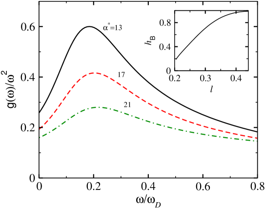
Figure 2: The reduced density of states $g(\omega)/\omega^{2}$ in units of $c^{3}$ ( $c$ is the sound speed) vs. $\omega/\omega_{D}$ corresponding to $\alpha\sigma^{2}$: 13 (solid), 17(dashed), 21(dot-dashed), for a hard sphere system at density of $\rho_{0}\sigma^{3}=1.1$. Inset shows corresponding boson peak height $h_{B}$ vs. localization length $\ell$ ($=1/\sqrt{\alpha}$).

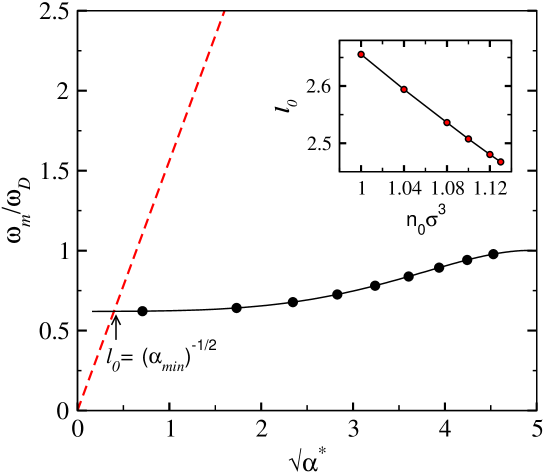
Figure 3: For a hard sphere system at density $\rho_{0}\sigma^{3}=1.1$, the ratio $\omega_{m}/\omega_{D}$ (see text) vs. $\sqrt{\alpha}\sigma$ (filled dots). Dashed line shows the upper limit of the frequency of the sound waves for localized the vibrational modes (see text). $\alpha_{\mathrm{min}}$ shown with an arrow is the minimum possible value of $\omega_{m}/\omega_{D}$ for the boson peak. Inset shows variation of $\ell_{0}$ ($=1/\sqrt{\alpha_{\mathrm{min}}}$ in units of $\sigma$ ) with density $\rho_{0}\sigma^{3}$ for the hard sphere system.

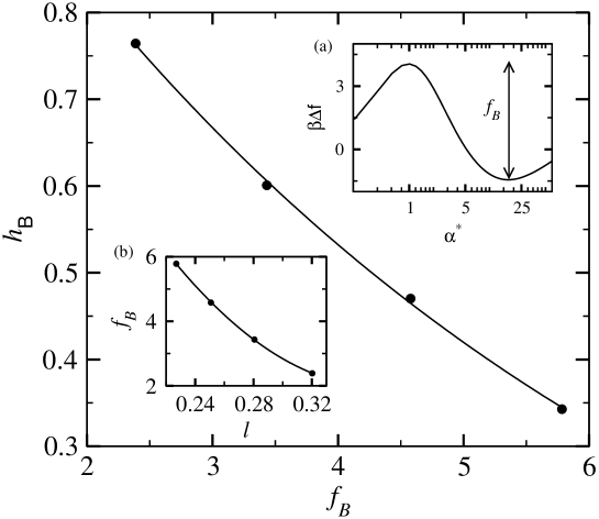
Figure 4: Boson peak height $h_{B}$ vs. the free energy barrier $f_{B}$ for the heterogeneous metastable states obtained in the $\alpha_{0}>\alpha$ region corresponding to different structures of a hard sphere system of $\rho_{0}\sigma^{3}=1.1$. Inset a) definition of $f_{B}$ and b) $f_{B}$ vs. the width $\ell$ of the gaussian density profiles.

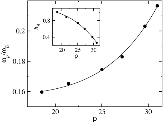
Figure 5: Ratio of frequency $\omega_{p}$ at the boson peak to the Debye frequency $\omega_{D}$ vs. pressure $P$ of the system ( in units of ${(\beta\sigma^{3})}^{-1}$). Inset shows height $h_{B}$ of the peak vs. pressure $P$.

References

- (1) R. C. Zeller, and R. O. Pohl, Phys. Rev. B 4, 2029 (1971).
- (2) A. Monaco et.al., Phys. Rev. Lett. 97, 135501 (2006).
- (3) D. A. Parshin, H. R. Schober, and V. L. Gurevich, Phys. Rev. B 76, 064206 (2007).
- (4) T. S. Grigera, V. Martin-Mayor, G. Parisi, and P. Verrocchio, Nature 422, 289 (2003).
- (5) E. Duval, A. Boukenter, and T. Achibat, J. Phys. Cond. Matt. 2, 0227 (1990)
- (6) V. Lubchenko and P. G.Wolynes, Proc. Natl. Acad. Sci. U.S.A. 100, 1515 (2003)
- (7) W. Schirmacher, G. Diezemann, and C. Ganter, Phys. Rev. Lett. 81, 136 (1998).
- (8) A. P. Sokolov, J. Phys.: Condens. Matter 11, A213 (1999).
- (9) W. Schirmacher, G. Ruocco, and T. Scopigno, Phys. Rev. Lett. 98, 025501 (2007)
- (10) M. T. Dove, M. J. Harris, A. C. Hannon, J. M. Parker, I. P. Swainson, and M. Gambhir, Phys. Rev. Lett. 78, 1070 (1997).
- (11) S. P. Das, Phys. Rev. E 59, 3870 (1999).
- (12) H. Shintani, H. Tanaka, Nat. Mater. 7, 870 (2008).
- (13) A. I. Chumakov et al. Phys. Rev. Lett. 106, 225501 (2011).
- (14) Reiner Zorn, Phys. Rev. B 81, 054208 (2010).
- (15) J. Goldstone, Nuovo Cim. 19, 15 (1961).
- (16) S. P. Das, Statistical Physics of Liquids at Freezing and Beyond, Cambridge University Press, NewYork, 2011.
- (17) P. Tarazona, Mol. Phys. 52, 871 (1984).
- (18) J. D. Bernal, Proc. R. Soc. London, Ser. A 280, 299 (1964).
- (19) Charles Bennett, J. Appl. Phys. 43, 2727 (1972).
- (20) Hartmut L wen, J. Phys. C 2, 8477 (1990).
- (21) C. Kaur, and S. P. Das, Phys. Rev. Lett. 86, 2062 (2001).
- (22) K. Kim, and T. Munakata, Phys. Rev. E, 68, 021502 (2003).
- (23) P. Chaudhary, S. Karmakar, C. Dasgupta, H.R. Krishnamurthy, A.K. Sood, Phys. Rev. Lett. 95, 248301 (2005).
- (24) Y. C. Shen and D. W. Oxtoby, J. Chem. Phys. 105, 6517 (1996).
- (25) S. N. Taraskin, Y. L. Loh, G. Natarajan, S. R. Elliott, Phys. Rev. Lett. 86, 1255 (2001).
- (26) T.V. Ramakrishnan, and M. Yussouff, 1979, Phys. Rev. B 19, 2775.
- (27) Henderson, D. and E. W. Grundke, J. Chem. Phys. 63, 601 (1975).
- (28) A. P. Sokolov, R. Calemczuk, B. Salce, A. Kisliuk, D. Quitmann, and E. Duval, Phys. Rev. Lett. 78, 2405 (1997).
- (29) C. A. Angell, Science 267, 1924 (1995)
- (30) T.R. Kirkpatrick, and P.G Wolynes, Phys. Rev. A 35, 3072 (1987).