Microscopic theory to quantify the competing kinetic processes in photoexcited surface-coupled quantum dots

Abstract

We present a self-contained theoretical and computational framework for dynamics following photoexcitation in quantum dots near planar interfaces. A microscopic Hamiltonian parameterized by first principles calculations is merged with a reduced density matrix formalism that allows for the prediction of time-dependent charge and energy transfer processes between the quantum dot and the electrode. While treating charge and energy transfer processes on an equal footing, the non-perturbative effects of sudden charge transitions on the Fermi sea of the electrode are included. We illustrate the formalism with calculations of an InAs quantum dot coupled to the Shockley state on an Au[111] surface, and use it to concretely discuss the wide range of kinetics possible in these systems and their implications for photovoltaic systems and tunnel junction devices. We discuss the utility of this framework for the analysis of recent experiments.

I Introduction

Nanostructured materials represent one of the most promising routes for the creation of novel energy harvesting and optoelectronic devices. One of the key challenges in this field is navigating the vast design space to search for an appropriate combination of material properties for a specific application. At present, the solution to this fundamental problem can at best be constructed for specific classes of systems. In the present paper, we tackle this problem for one of the key configurations that has emerged in the fields of photovoltaics and nanoelectronics: quantum dots acting as chromophores in the vicinity of semiconductor and metallic surfaces (Tisdale et al., 2010; Choi et al., 2010; Kleemans et al., 2010).

We focus on charge kinetics in these systems and construct a microscopic dynamical theory that is capable of both describing the observable experimental phenomena, and of making quantitative predictions for future research. The key challenge addressed in the paper is the construction of a framework in which a strong connection is maintained between the microscopic parameterization of the Hamiltonian, and the description of dynamics within a restricted set of excited states. Thus key insights from an efficient navigation of the parameter space can be related to specific physical properties of the underlying materials in these systems.

Theories based on model Hamiltonians (Fainberg et al., 2011; Galperin et al., 2009; May and Kühn, 2008; Fainberg et al., 2007; Galperin and Nitzan, 2005) allow one to construct a picture of the possible regimes of dynamics, but the connection to realistic modeling of specific materials may be hard to establish. On the other hand, parameter free ab-initio studies (Kanai et al., 2010; Prezhdo et al., 2009) can only address relatively small systems and the key physical features of quantum dot systems can not be treated. The work presented in this paper may be viewed as a compromise between these two extremes. Starting from the fundamental many-body Hamiltonian for the light-matter interaction, we derive a low energy effective Hamiltonian in which all matrix elements are calculated from the single particle wavefunctions of the subsystems, each represented by a well-established model. The wavefunctions and other characteristics of the surface are obtained from an ab-initio Density Functional Theory based calculation. The frontier states in the semiconductor quantum dot are obtained from established effective mass models. In the region of overlap between these subsystems, these wavefunctions can be treated on equal footing. In this way, our low energy effective Hamiltonian is fully derived, with the addition of no parameters. This Hamiltonian is then used to develop a master equation for the reduced dynamics of the quantum dot. Simulations based on the master equation provide quantitative analysis of the range of possible charge kinetics in these systems with a clear connection to the constituent surface and quantum dot materials.

By constructing the Hamiltonian in this way, a meaningful analysis of charge and energy transfer channels in isolation and in competition with each other emerges. Thus one can pursue important questions about charge kinetics such as: How does the extinction of optical power by the quantum dot change in the presence of a surface? How is cooling of hot carriers affected by the presence of energy transfer to the surface? How does electrostatic coupling of the quantum dot to a surface affect the lifetime of exciton, bi-exciton, and other multi-electron states? How does non-radiative recombination of excitons in these systems affect current extraction and photoluminescence? Our framework is capable of answering these questions concretely. We illustrate this within a specific system of InAs quantum dot on a gold surface.

In recent years, several studies of kinetic processes in models for single molecule junctions under the influence of both applied electrical bias and optical fields have been published Kanai et al. (2010); Galperin and Nitzan (2005); Galperin et al. (2009); van der Molen et al. (2009); Petrov et al. (2011); Prezhdo et al. (2009); Fainberg et al. (2011, 2007); May and Kühn (2008); Bergfield and Stafford (2009). The studies of asymmetric dipole coupling in the steady state conductance Galperin and Nitzan (2005); Galperin et al. (2009) have revealed photo-induced current generation, and current induced photo-emission. This scenario, however, is inapplicable to single interface systems in which only a photo-generated current can can exist, and interfacial polarization plays a different role, as described below. Electron dynamics in molecular chromophores at semiconductor interfaces has been studied in depth for a small number of systems and ideal situations fully ab-initioPrezhdo et al. (2009). While these studies are invaluable for quantitatively settling many questions about the microscopic processes and their dynamical interplay, they do not capture the aspects arising from the relatively large sizes of quantum dots. Furthermore, the treatment of image potential at the interface remains an external input to any computation based purely on density functional theoryChulkov et al. (1999); Neaton et al. (2006); Garcia-Lastra et al. (2009).

The highly polarizable surfaces of the planar electrode and the quantum dot lead to electrostatic interactions that significantly affect the quasiparticle and optical bandgaps, tunneling rates, as well as energy transfer. For a spherical quantum dot, an important fundamental effect of the presence of a planar surface is the formation of a dipole moment and strong corrections to multipole moments of its exciton states. Thus, the polarizability of electrode surface becomes a mechanism for non-radiative recombination of excitons via energy transfer to the electrode. In our numerical results, we show the effects of this polarizability and quantify the significance of high order multipole moments of charge distribution on the non-radiative exciton recombination in the narrow gap InAs quantum dot. Having a microscopic Hamiltonian in hand further allows us to compare this exciton decay with the dissociation across the junction. This type of analysis, for example, is fundamental to optimization of current extraction in photovoltaic applications of these systems.

Furthermore, the size of a quantum dot also yields many closely spaced energy levels, which lead to dynamical effects that often do not arise in single molecules, especially if a simplified treatment is limited to just the highest occupied and lowest unoccupied molecular orbital. The spacing and the number of energy levels qualitatively affects the dynamics of charge injection, energy exchange, and the recoil of a hole (electron) in response to the tunneling of an electron (hole) to the electrode. Understanding the time for build-up of these transitions in relation to the magnitude of these transition rates is fundamental to determining the regimes where a Markovian description of charge and energy transfer breaks down. In experimental terms, it allows us to understand when to expect deviations from Lorentzian lineshapes in both linear absorption and non-linear optical spectroscopy of these systems. The non-Markovian effects originate physically from the coupling of quantum dot states to the electrode, as has also been discussed by Fainberg et al. Fainberg et al. (2011) in the case of molecular junctions. However, it can be affected significantly by the spacing of energy levels in the quantum dot, which is a complementary aspect that exists naturally in our work. Furthermore, the levels also couple significantly, via the Coulomb interaction, to the incoherent particle-hole excitations in the Fermi sea of the electrode, which opens additional channels of energy transfer beyond those discussed in studies of molecular systems.

With a few notable exceptionsFainberg et al. (2011); Sukharev and Galperin (2010); Elste et al. (2011), studies in molecular transport generally treat the electrodes as passive Fermionic reservoirs, thus ignoring the scattering of electrons in the leads as a result of the excitation dependent Coulomb potential of the molecule. Under certain conditions, discussed in this paper, this potential can significantly alter the transport and relaxation in tunneling junctions Matveev and Larkin (1992); Abanin and Levitov (2004, 2005); Segal et al. (2007), as well as the optical absorptionDespoja et al. (2008). For example, tunneling of an electron out of the quantum dot yields sudden transition of its charge, and can cause significant dynamical fluctuations in the surface charge density in the electrode. Studies of the effects of this kind have a long history in X-ray emission and absorption in bulk metals, and optical absorption in doped quantum wellsHawrylak (1991a); Skolnick et al. (1987); Schmitt-Rink et al. (1989) They are well-known to be composed of two competing contributions: the Mahan exciton (ME)Mahan (1967, 1980, 2000); Ohtaka and Tanabe (1990) arising from the attraction of the electron in the Fermi sea to the hole, and the Anderson orthogonality catastrophe (AOC)Anderson (1967); Ohtaka and Tanabe (1990) arising from the vanishing overlap between the initial and the final many-body state. Together they define the phenomenon of the Fermi edge singularity (FES). A highly relevant example to the systems considered in this paper is the recent observation of ME in InGaAs/GaAs quantum dot heterostructuresKleemans et al. (2010).

The theory formulated in this paper fully accounts for FES phenomenon self-consistently alongside charge and energy transfer processes. A novel aspect of the geometry considered in this paper is that it is ideal for exploring FES within the hole bands of a p-doped electrode. This has remained unexplored in FES studies in bulk metals and quantum wells because the core charge in this case is the much lighter electron, the motion of which diminishes the FES signature. On the other hand, the electron localized inside the dot presents no such problem and new effects arising from scattering in non-parabolic bands and the much larger sub-band mixing in hole states can be explored. In addition, identifying systems in which these effects yield important signatures in optical response and tunneling current is important for the correct interpretation of experimental data as well as device engineering.

The FES has also been studied in resonant tunneling devicesMatveev and Larkin (1992), and was first predicted in these systems by Matveev and Larkin Matveev and Larkin (1992). Abanin et al. emphasized the tunability of the FES effect by engineering the geometric aspects of the system, and elucidated the novel effects arising within a non-equilibrium electron gasAbanin and Levitov (2005). The optical response we formulate here naturally leads to an extension of this idea within the interfacial quantum dot systems where tuning the relative effect of the ME against the AOC can be achieved by controlling whether the final state of the optical excitation lies in the Fermi sea or in the capping layer of the heterostructure.

In a study by Despoja et alDespoja et al. (2008) on the ab-initio calculations of the core-hole spectrum of jellium surfaces the FES was found to be very weak for a core-hole residing outside the surface. This is due to very strong screening by the free electron gas in the metal. While this may be expected for the small overlap between the sharply screened potential inside the metal, and the extended states of the slab, our numerical calculations show it to be true even for the sea of Shockley surface states on Au[111]. On the other hand, we expect the effect to increase dramatically for thin films supported on an insulating substrate with low dielectric constant.

Our paper is organized as follows: in Sec. II we derive the microscopic Hamiltonian. The detailed expressions for all the required Hamiltonian matrix elements are provided in Appendix A. In Sec. III, we develop our model for the dynamics, specifically a time-convolutionless master equation for the density matrix of the quantum dot. From this equation, we obtain the dynamical rates of charge and energy transfer, as well as the optical response including the effects of the FES. In Sec. IV we apply our model to calculations of charge and energy transfer for an InAs quantum dot on Au[111] surface, and study the effect of the FES as well as the competition between tunneling, cooling, and non-radiative exciton decay on the dynamics. In Sec. V we discuss the application of our theory to the modeling and analysis of experiments, and the possible extension of the theory developed here to that of a quantum dot array supporting inter-dot charge and energy transport. We also discuss in this section how the vibrational modes of the quantum dot, neglected in the explicit analysis, can be described within the framework presented. In Sec. VI we conclude. Details not found in the text may be found in Appendices A and B.

II Microscopic Hamiltonian

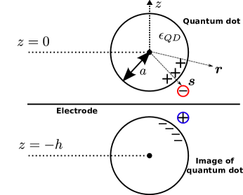
(a)

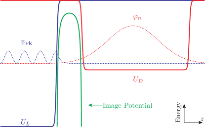
(b)

Figure 1: (a) The geometry of the system studied in this paper showing the important parameters for determining the electrostatic potentials. (b) Schematic profile of potentials and wavefunctions of the electrode and the quantum dot in a plane perpendicular to the electrode surface and passing through the center of the dot.

We start with the Hamiltonian,

$$H(t) = \int d\boldsymbol{r}\,\Psi^{\dagger}(\boldsymbol{r})\left[\frac{1}{2m}\left(\frac{\hbar}{i}\nabla+e\mathbf{A}(\boldsymbol{r},t)\right)^{2}\right]\Psi(\boldsymbol{r})$$

$$+\int d\boldsymbol{r}\,\Psi^{\dagger}(\boldsymbol{r})\left[U_{D}(\boldsymbol{r})+U_{L}(\boldsymbol{r})\right]\Psi(\boldsymbol{r})$$

$$+\frac{1}{2}\int d\boldsymbol{r}\int d\boldsymbol{r}^{\prime}\,\Psi^{\dagger}(\boldsymbol{r})\,\Psi^{\dagger}(\boldsymbol{r}^{\prime})V(\boldsymbol{r}-\boldsymbol{r}^{\prime})\Psi(\boldsymbol{r}^{\prime})\Psi(\boldsymbol{r}),$$

where $\Psi(\boldsymbol{r})$ is the fermionic annihilation field operator. The interaction of electrons with light occurs through the vector potential $\mathbf{A}(\boldsymbol{r},t)$ associated with the optical field. We treat the field as a classical external force in this work. Therefore we do not include energy stored in this field in the above Hamiltonian. The potentials associated with the QD and the electrode are given by the functions $U_{D}(\boldsymbol{r})$ and $U_{L}(\boldsymbol{r})$ respectively (see also Fig. 1). In the last term of (II) $V(\boldsymbol{r}-\boldsymbol{r}^{\prime})$ is the Coulomb interaction among all fermions. We have neglected the phonons and electron-phonon interaction in the present model for brevity, but it can be incorporated straightforwardly in our formalism, and we comment in Section IV on how this can be accomplished.

Our approach is akin to the Bardeen approach to tunneling Bardeen (1961). We make a physically reasonable distinction between states of the QD and the electrode, and then develop a theory for the charge and energy exchange between the two sets of states. It is then convenient to first write the field operator as a sum of field operators that create/annihilate particles confined to the QD and the electrode,

$$\Psi(\boldsymbol{r})=\Psi_{D}(\boldsymbol{r})+\Psi_{L}(\boldsymbol{r}).$$ (2)

With the choice of the single particle basis below, how the states within the two subsystems can be identified will be detailed. It is implicit in the formalism of the reduced dynamics of the QD (see Sec. III) that the electrode states, which are traced over, are orthogonal to the QD states included in the dynamics. Any distinction based on exact vanishing of the states within appropriately defined volumes of the two subsystems would not yield an orthogonal basis in general Prange (1963). However, with the barrier potential equal to several electron volts, the low energy states of the QD and those near the Fermi level of the electrode, even when calculated in isolation of each other, decay exponentially within the barrier with a characteristic length of about 1-2 Å. The QD and electrode states most relevant to the dynamics are then orthogonal to a good approximation. We exploit this property in the calculations, but note that the approximation lies in the choice of basis and not in the formalism.

We substitute (2) into the Hamiltonian (II) above, and group the terms as follows,

$$H_{D} = \int d\boldsymbol{r}\Psi_{D}^{\dagger}(\boldsymbol{r})\left[\frac{1}{2m}\left(\frac{\hbar}{i}\nabla+e\mathbf{A}(\boldsymbol{r},t)\right)^{2}+U_{D}(\boldsymbol{r})+U_{L}(\boldsymbol{r})\right.+\left.\int d\boldsymbol{r}^{\prime}V(\boldsymbol{r}-\boldsymbol{r}^{\prime})\left\{\Psi_{D}^{\dagger}(\boldsymbol{r}^{\prime})\Psi_{D}(\boldsymbol{r}^{\prime})+\rho_{img}(\boldsymbol{r}^{\prime})\right\}\right]\Psi_{D}(\boldsymbol{r}),$$ (3)

$$H_{L} = \int d\boldsymbol{r}\Psi_{L}^{\dagger}(\boldsymbol{r})\left[\frac{1}{2m}\left(\frac{\hbar}{i}\nabla+e\mathbf{A}(\boldsymbol{r},t)\right)^{2}+U_{D}(\boldsymbol{r})+U_{L}(\boldsymbol{r})+\int d\boldsymbol{r}^{\prime}V(\boldsymbol{r}-\boldsymbol{r}^{\prime})\Psi_{L}^{\dagger}(\boldsymbol{r}^{\prime})\Psi_{L}(\boldsymbol{r}^{\prime})\right]\Psi_{L}(\boldsymbol{r}),$$ (4)

$$H_{DL} = \int d\boldsymbol{r}\Psi_{D}^{\dagger}(\boldsymbol{r})\left[\frac{1}{2m}\left(\frac{\hbar}{i}\nabla+e\mathbf{A}(\boldsymbol{r},t)\right)^{2}+U_{D}(\boldsymbol{r})+U_{L}(\boldsymbol{r})\right]\Psi_{L}(\boldsymbol{r}),$$ (5)

$$V_{DL} = \int d\boldsymbol{r}\int d\boldsymbol{r}^{\prime}\Psi_{D}^{\dagger}(\boldsymbol{r})\Psi_{D}(\boldsymbol{r})V(\boldsymbol{r}-\boldsymbol{r}^{\prime})\left[\Psi^{\dagger}_{L}(\boldsymbol{r}^{\prime})\Psi_{L}(\boldsymbol{r}^{\prime})-\rho_{img}(\boldsymbol{r}^{\prime})\right].$$ (6)

The term $H_{D}$ given by (3) describes the QD states in the presence of the electrode potential, the Coulomb interaction among carriers, and the classical electrostatic interaction with the electrode in the form of an image potential. The latter is included via the induced density (a real-valued function) $\rho_{img}(\boldsymbol{r})$, which is later subtracted in (6). We call the basis states of $H_{D}$ for $\mathbf{A}=0$ the QD states, and the matrix elements of $-im^{-1}\hbar\mathbf{A}(\boldsymbol{r})\cdot\nabla$ between these states defines the optical excitation of the QD in the presence of an electrode.

Similarly, $H_{L}$ in (4) defines electrode states and their optical interaction in the presence of the lattice potential $U_{L}$ and the Coulomb interaction among carriers. The single particle states of $H_{L}$ are calculated with full atomic scale detail, after setting $\mathbf{A}=0$. Then the Coulomb interaction appearing in Eq. (4) is incorporated into the treatment of the states at the level captured by Density Functional Theory. In the particular example we use for illustration, only the surface bound states play a direct role in calculations, while the remaining states are kept formally for completeness. In the final reduced dynamics of the QD, the sum of the interaction matrix elements over these states yields well-defined single and two-particle response functions. The actual problem of treating the electrode is then reduced to the calculation of these response functions in the presence of a surface. The surface bound states are calculated by constructing the surface Green functions from the Kohn-Sham density functional theory, as discussed at length in Section IV.

Next, the term $H_{DL}$ given by (5) describes hybridization, including the optically driven excitations in which an electron or a hole is excited directly into a final state in the electrode. This term thus describes charge transfer. The last term, $V_{DL}$, given by (6), describes energy transfer mediated by the Coulomb interaction between the QD and the electrode. The advantage of adding and subtracting $\rho_{img}(\boldsymbol{r})$ in the above expressions is two fold: the QD states include the image potential non-perturbatively, and the dynamical interaction of these states with the electrode reduces to fluctuations around this density. As we will see in Section III.3, this naturally leads to describing the energy transfer in terms of a dynamical longitudinal susceptibility of the electrode.

In the above expansion we neglect the term $\Psi^{\dagger}_{L}(\boldsymbol{r})U_{D}(\boldsymbol{r})\Psi_{L}(\boldsymbol{r})$ that appears in $H_{L}$, which would result in additional renormalization of the electrode states in response to the presence of the neutral QD. We disregard this term because the exponential decay of the electrode wavefunctions in the barrier, combined with the extended nature of these wavefunctions inside the electrode, makes the effect of this perturbation very small. On the other hand, the changes induced by the presence of the electrode has a significant effect on the boundary conditions for the states localized to the QD, and thus the analogous term $\Psi_{D}^{\dagger}(\boldsymbol{r})U_{L}(\boldsymbol{r})\Psi_{D}(\boldsymbol{r})$ is included in the $H_{D}$ term. We remark that the neglected term may be included by calculating the scattering states starting from the eigenstates of $H_{L}$ Mahan (2000). This would perhaps be necessary for some mesoscopic electrodes lying at a very small distance from the QD, or in cases with small barrier heights such that the electrode wavefunctions significantly probe $U_{D}(\boldsymbol{r})$.

We have also neglected the particular exchange interaction where one carrier lies in the QD state, and the other in the electrode state. This interaction should also be exponentially suppressed for the low energy and well confined states of relevance to this work. Related to this exchange is the Coulomb-driven tunneling process which is also neglected in comparison to the contribution by single particle kinetic and potential energies as well as optical interactions, $H_{DL}$. The exchange interaction among carriers within each subsystem is implicit in the above expressions.

Let us now turn to specification of the states comprising $\Psi_{D}$ and $\Psi_{L}$, and begin with a set of single particle basis states. Let $\left|g\right\rangle$ be the ground state of the QD, and $\varphi_{n}(\boldsymbol{r})=\left\langle\boldsymbol{r}\left|\right.n\right\rangle$ be the single particle excited states satisfying,

$$\left[-\frac{\hbar^{2}}{2m_{0}}\nabla^{2}+U_{Deff}(\boldsymbol{r})+\Sigma(\boldsymbol{r})-\varepsilon_{n}\right]\varphi_{n}(\boldsymbol{r})=0.$$ (7)

Here $U_{Deff}$ represents the pseudopotential for a single electron or a hole added to the neutral ground state of the QD, and we have introduced the electrostatic self energy of a point charge in the vicinity of polarizable surfaces such as that of the QD and the electrode. The electrode contribution is given by Virk et al. (2012)

$$\Sigma_{L}(\boldsymbol{r})=\int d\boldsymbol{r}^{\prime}V(\boldsymbol{r}-\boldsymbol{r}^{\prime})\rho_{img}(\boldsymbol{r}^{\prime}).$$ (8)

This is a well-known formulation of an exact one-body potential representing the electrostatic energy stored in the polarization reaction field that is induced by a unit charge on dielectric surfaces Bányai et al. (1992); Böttcher and van Belle (1973); Brus (1984).

We label the solutions to the eigenvalue equation (7) as electron states, $\varphi_{e}(\boldsymbol{r})$, for the addition of a single electron to the QD state $e$ above the quasi-particle energy gap, and hole states, $\varphi_{h}^{*}(\boldsymbol{r})$, for the removal of an electron from a valence state, $h$. While the solutions at higher energies significantly violate the boundary conditions at the electrode surface, they are nonetheless useful in forming a convenient basis set for expanding the multi-particle states. The present paper discusses only the exciton as the multi-particle excitation, and we express its wavefunction as,

$$\Phi_{x}(\boldsymbol{r}_{e},\boldsymbol{r}_{h})=\sum_{eh}\varphi_{e}(\boldsymbol{r}_{e})\varphi_{h}^{*}(\boldsymbol{r}_{h})\Phi_{eh;x},$$ (9)

where the coefficients $\Phi_{eh;x}$ are determined from a variational calculation including the Coulomb interaction between the electron, hole, and their induced surface polarizations (see (3) and Sec. IV). This approach has been employed widely in semiconductor opticsHu et al. (1990); Chuang et al. (1991).

The electrode states diagonalize $H_{L}$ in  (4) for $\mathbf{A}=0$, and we write them as $\psi_{\nu\boldsymbol{k}}=u_{\nu\boldsymbol{k}}(\boldsymbol{r})e^{i\boldsymbol{k}\cdot\boldsymbol{r}}$. While it is not essential for the theory presented, we have parameterized these states by a two-dimensional quasi-momentum $\boldsymbol{k}$, thus assuming that the electrode has a planar surface. In a semi-infinite electrode, $\nu$ may also take continuous values within regions of the bulk excitations in the projected density of states. In terms of the (non-orthogonal) basis set above, (2) can now be written more precisely as,

$$\Psi(\boldsymbol{r}) = \sum_{n}\varphi_{n}(\boldsymbol{r})c_{n}+\sum_{\nu\boldsymbol{k}}u_{\nu\boldsymbol{k}}(\boldsymbol{r})e^{i\boldsymbol{k}\cdot\boldsymbol{r}}c_{\nu\boldsymbol{k}},$$ (10)

where the first term on the right hand side corresponds to $\Psi_{D}$ and the second to $\Psi_{L}$. The operators $c_{n}$ and $c_{\nu\boldsymbol{k}}$ annihilate particles in states $\varphi_{n}$ and $\varphi_{\nu\boldsymbol{k}}$ respectively. The sum over $n$ is truncated to states that are well localized on the QD in the sense that their weight in the electrode region is negligible. The remaining states, which are high in energy and have a significant fraction of their wavefunction inside the electrode, are then all viewed formally as part of the states to be traced over in the reduced dynamics.

Separating the optical interaction from the $\mathbf{A}=0$ form of the terms in (3)-(6), we now write the Hamiltonian as

$$H=H_{D}+H_{L}+H_{T}+V_{C}+H_{D}^{(r)}+H_{L}^{(r)}+H_{T}^{(r)},$$ (11)

in which the first two terms are the Hamiltonians for the quantum dot and the electrode states in the absence of radiation,

$$H_{D} = \sum_{n}\left|n\right\rangle\varepsilon_{n}\left\langle n\right|,$$ (12)

$$H_{L} = \sum_{\nu\boldsymbol{k}}\varepsilon_{\nu\boldsymbol{k}}c_{\nu\boldsymbol{k}}^{\dagger}c_{\nu\boldsymbol{k}}.$$ (13)

Here the $\varepsilon_{n}$ are the energies of the QD states, including the ground state of the neutral QD, single electron and hole states, and the neutral exciton states. The $\varepsilon_{\nu\boldsymbol{k}}$ are the dispersion of electrode energies with band index $\nu$. The third term in (11), which arises from (5) represents the hybridization between the QD and the electrode, and we write it as,

$$H_{T} = \left|e\right\rangle\left\langle g\right|\mathcal{T}^{eg}+\left|h\right\rangle\left\langle g\right|\mathcal{T}^{hg}$$ (14)

$$+\left|h\right\rangle\left\langle x\right|\mathcal{T}^{hx}+\left|e\right\rangle\left\langle x\right|\mathcal{T}^{ex}+c.c.$$

Here we have introduced the electron transfer operators, $\mathcal{T}^{ab}$, corresponding to the tunneling induced change in the charge state of the quantum dot. These formal operators are introduced to simplify the dynamical model in Sec. III below, and are defined as,

$$\mathcal{T}^{eg} = \sum_{\nu\boldsymbol{k}}T^{eg}_{\nu\boldsymbol{k}}c_{\nu\boldsymbol{k}},$$ (15)

$$\mathcal{T}^{hg} = \sum_{\nu\boldsymbol{k}}T^{hg}_{\nu\boldsymbol{k}}c_{\nu\boldsymbol{k}}^{\dagger},$$ (16)

$$\mathcal{T}^{hx} = \sum_{\nu\boldsymbol{k}}T^{hx}_{\nu\boldsymbol{k}}c^{\dagger}_{\nu,\boldsymbol{k}},$$ (17)

$$\mathcal{T}^{ex} = \sum_{\nu\boldsymbol{k}}T^{ex}_{\nu\boldsymbol{k}}c_{\nu\boldsymbol{k}}.$$ (18)

The matrix elements $T^{aa^{\prime}}_{\nu\boldsymbol{k}}$ represent tunneling amplitudes, and can be computed from the electronic states $\varphi_{n}$ and $\psi_{\nu\boldsymbol{k}}$ as described in detail in Appendix A. Recall that $\varphi_{h}$ represents a single electron orbital in the valence band , such that $\varphi_{h}^{*}$ is the state of the corresponding hole. Thus the matrix element $T^{hg}_{\nu\boldsymbol{k}}$ describes the transfer of an electron from state $h$ in the valence band of the QD to the electrode. We have now defined all the electron transfer operators needed for the formalism below to describe addition or removal of electrons from the QD.

Returning to (11), the fourth term represents the Coulomb interaction in (6), which we expand in QD basis states,

$$V_{C} = \sum_{nm}\left|n\right\rangle\left\langle m\right|\hat{V}_{nm},$$ (19)

where the operator $\hat{V}_{nm}$ acts on the electrode states, and is defined as

$$\hat{V}_{nn^{\prime}} = \sum_{\nu,\nu^{\prime}}\sum_{\boldsymbol{k},\boldsymbol{k}^{\prime}}V_{n,\nu\boldsymbol{k};n^{\prime},\nu^{\prime}\boldsymbol{k}^{\prime}}c_{\nu\boldsymbol{k}}^{\dagger}c_{\nu^{\prime}\boldsymbol{k}^{\prime}}.$$ (20)

The matrix elements in this expression follow directly from (6), and are defined in full form in (A.2). For $n\neq m$, the $\hat{V}_{nm}$ represent quantum fluctuations around the classically induced density of the electron gas and lead to energy and polarization transfer between the QD and the electrode. On the other hand, the diagonal terms, $\hat{V}_{nn}$, cause random fluctuations in the energy level of the QD. This may be thought of as a back-action from the excitations in the electrode induced by the QD potential. As was discussed in the Introduction, this coupling results in the FES and AOC phenomena.

At this stage we let $\hat{V}_{nm}$ represent all electronic excitations of the system so that the matrix elements may be taken to be the bare Coulomb interaction. In actual calculations, however, it is more convenient to identify a set of elementary excitations of the electrode strongly coupled to the QD, and then renormalize this coupling by the interactions among these excitations, and their interactions with the weakly coupled excitations. We will see in Sec. III that this can be achieved essentially by defining a frequency dependent dielectric function for the electrode surface, in which the relevant interactions are included by construction.

We now turn to the last three terms of (11), which describe the interaction of the entire system with the external electromagnetic (EM) field. We first write the matrix elements of the velocity operator in the standard form as,

$$\mathbf{v}_{nn^{\prime}}(t) = \frac{e}{2m}\mathbf{A}(t)\delta_{nn^{\prime}}$$

$$+\frac{\hbar}{2mi}\int d\boldsymbol{r}\left[\phi_{n}^{*}(\boldsymbol{r})\nabla\phi_{n^{\prime}}(\boldsymbol{r})-\phi_{n^{\prime}}(\boldsymbol{r})\nabla\phi_{n}^{*}(\boldsymbol{r})\right],$$

where $\phi_{n}$ may be set to a QD state $\varphi_{n}$ or an electrode state $\psi_{\nu}$. The fundamental optical transition is the exciton, and we define its matrix element as,

$$\mathbf{v}_{xg}(t) = \sum_{e,h}\mathbf{v}_{eh}(t)\Phi_{eh;x},$$ (22)

and write the interaction between the EM field and the QD as,

$$H_{D}^{(r)}(t) = e\sum_{x}\mathbf{A}(t)\cdot\mathbf{v}_{xg}(t)\left|x\right\rangle\left\langle g\right|+\mbox{c.c}.$$ (23)

Similarly the interaction between the electrodes and the EM field is given by

$$H_{L}^{(r)}(t) = e\sum_{\nu,\nu^{\prime}}\sum_{\boldsymbol{k},\boldsymbol{k}^{\prime}}\mathbf{A}(t)\cdot\mathbf{v}_{\nu\boldsymbol{k},\nu^{\prime}\boldsymbol{k}^{\prime}}(t)c_{\nu\boldsymbol{k}}^{\dagger}c_{\nu^{\prime}\boldsymbol{k}^{\prime}}+\mbox{c.c.}\;\;$$ (24)

An additional light-matter coupling that we do not consider in much detail here, $H_{T}^{(r)}$, describes the radiation driven charge transfer between the QD and the electrode. This term introduces an externally controllable exciton dissociation between the QD and the electrode, and takes the form,

$$H_{T}^{(r)}(t) = e\sum_{e}\left|e\right\rangle\left\langle g\right|\sum_{\nu\boldsymbol{k}}\mathbf{A}(t)\cdot\mathbf{v}_{e;\nu\boldsymbol{k}}(t)c_{\nu\boldsymbol{k}}$$

$$-e\sum_{h}\left|h\right\rangle\left\langle g\right|\sum_{\nu\boldsymbol{k}}\mathbf{A}(t)\cdot\mathbf{v}_{h;\nu\boldsymbol{k}}(t)c_{\nu\boldsymbol{k}}^{\dagger}+\mbox{c.c.}$$

This completes our construction of the microscopic Hamiltonian, and we now turn to the description of the charge dynamics of an electrode coupled quantum dot.

III Dynamics following photo-excitation

We study dynamics within the restricted Hilbert space of four classes of states: the ground state $\left|g\right\rangle$, single electron states, $\left|e\right\rangle$, single hole states $\left|h\right\rangle$, and the exciton states $\left|x\right\rangle$. This restriction is only for convenience, and may be lifted by expanding the set to include bi-exciton states and even larger multi-electron complexes. Within each class, however, we do allow for an arbitrary number of states to exist. Since this system is coupled to the electrodes, the unitary evolution governed by the Schrödinger equation applies to the full density matrix, which we denote as $\xi(t)$, and it obeys the equation,

$$\frac{d}{dt}\xi(t) = \frac{-i}{\hbar}\left[H(t),\xi(t)\right],$$ (26)

where $H(t)$ is the Hamiltonian (11) discussed in the previous section. Fundamentally, the equation describes optical excitations acting as the external force driving the system out of equilibrium (the last three terms in (11)), and the dynamical couplings between QD and electrodes returning the two subsystems towards a state of mutual equilibrium (via both $H_{T}$ and $V$). Assuming that the electrode stays in equilibrium, we now reduce this equation to the description of excitation, dephasing, and relaxation of the QD alone.

III.1 Reduced density matrix dynamics

Recent experiments have pinpointed subtle FES effects in optical spectra of quantum dots coupled to quantum wells Latta et al. (2011); Kleemans et al. (2010); Türeci et al. (2011). Thus it is crucial to include the effects of FES in our theory. In order to achieve this, a special interaction picture must be constructed to fully account for the non-perturbative scattering of the electrode states in response to the electrostatic potential of the QD. Our approach is motivated by the one body formulation of the X-ray spectra by MahanMahan (1980), Nozieres and De DominicisNozières and De Dominics (1969), and the analysis of orthogonality catastrophe by AndersonAnderson (1967). In the original FES papers, the authors captured how the sudden shift in the Hamiltonian of electrons forming a Fermi sea affects the photoemission and absorption spectra in metallic systemsMahan (1967). Following this work, investigations into the FES in the photo-excitation of doped semiconductors were also carried outHawrylak (1991a). We also note the studies of the FES within the context of pump-probe experiments sensitive to the coherent non-linear optical response of doped semiconductorsPrimozich et al. (2000); Perakis and Shahbazyan (2000). All these works focus on changes in the lineshape of the optical spectrum of a Fermi sea.

Here we explore the consequences of these fundamental effects in the exciton dissociation across a QD-electrode interface. We formulate a master equation for an electrode coupled QD, and show how the effects of FES can be introduced in this theory, and how they can be re-captured naturally in the time-dependent couplings defining the resulting equation. Thus the FES becomes an integral part of the dynamical map that propagates the state of the QD towards equilibrium. The couplings in which the FES appears take the form of correlation functions bearing many similarities to the results of Nozieres and De DominicisNozières and De Dominics (1969). However, our equations address a very different physical scenario, and they are applied without making any simplifying assumptions on the spatial profiles of the different electrostatic potentials created by QD states. We also develop one-body formulas for calculating and interpreting these correlation functions. We will first discuss the derivation of the equation of motion for a general electrode, and then specialize to the case of a Fermionic reservoir.

III.1.1 Derivation of the general form

From the full Hamiltonian defined in (11) in which the Coulomb interaction is given by (19), we take three contributions to construct the interaction picture by defining a Hamiltonian,

$$H_{0} \equiv H_{D}+H_{L}+\sum_{n}\hat{V}_{nn}\left|n\right\rangle\left\langle n\right|,$$ (27)

where $n$ is a label for the QD states. The last term in the expression above scatters electrode states via a potential that is conditioned upon the QD state. This term is also the key to capturing the FES effects, but it complicates the interaction picture by yielding a non-perturbative coupling between the system and the bath.

An analogue of this way of partitioning the Hamiltonian has been used in the chemical physics literature in the pastZhang et al. (1998); Yang and Fleming (2002); Golosov and Reichman (2001). Such a reference system leads to the so called “modified Redfield” approaches Zhang et al. (1998); Yang and Fleming (2002). The crucial difference here is that our bath is composed of fermionic excitations, which alter both the physics and the formalism compared to the bosonic vibrational degrees of freedom at play in the previous work.

To proceed with our analysis, we define the full density matrix within our interaction picture as,

$$\tilde{\xi}(t)=e^{iH_{0}t/\hbar}\xi(t)e^{-iH_{0}t/\hbar}.$$ (28)

In the Schrödinger picture, the reduced density matrix defined only over the QD states can be obtained by tracing $\xi(t)$ over the electrode degrees of freedom. However, we begin with a slightly different version of this procedure and relate the reduced density matrix in the Schrödinger picture to the $\tilde{\xi}(t)$ via the equation,

$$\rho(t)=\mbox{Tr}_{L}\left[e^{-iH_{0}t/\hbar}\tilde{\xi}(t)e^{iH_{0}t/\hbar}\right].$$ (29)

The FES arises when many body states are subjected to unitary rotation by two (or more) different Hamiltonians. The exponentials in the above formula accomplish this exactly, and allow us to expand the remaining interactions between QD and the electrode perturbatively. From the chemical physics perspective, the exponentials take into account the bath-induced random fluctuations of the QD energy levels, which cause the phenomenon of pure dephasing (decoherence without population relaxation)Golosov and Reichman (2001); Hsu and Skinner (1985).

Returning to the general derivation, we write the Schrödinger equation within the interaction picture as

$$\frac{d}{dt}\tilde{\xi}(t) = -\frac{i}{\hbar}\left[H_{T}(t),\tilde{\xi}(t)\right]-\frac{i}{\hbar}\left[V_{C}(t),\tilde{\xi}(t)\right]$$

$$-\frac{i}{\hbar}\left[H_{D}^{(r)}(t),\tilde{\xi}(t)\right]-\frac{i}{\hbar}\left[H_{L}^{(r)}(t),\tilde{\xi}(t)\right]$$

$$-\frac{i}{\hbar}\left[H_{T}^{(r)}(t),\tilde{\xi}(t)\right].$$

The formal solution of this equation in the absence of an external electromagnetic field may be written as,

$$\tilde{\xi}(t)=T_{+}\exp\left(-i\int_{0}^{t}dt^{\prime}\mathcal{J}_{I}(t^{\prime})\right)\xi(0).$$ (31)

The symbol $T_{+}$ enforces time ordering such that

$$T_{+}\exp\left(-i\int_{0}^{t}dt^{\prime}\mathcal{J}_{I}(t^{\prime})\right) = 1-i\int_{0}^{t}dt^{\prime}\mathcal{J}_{I}(t^{\prime})$$

$$-\int_{0}^{t}dt^{\prime}\int_{0}^{t^{\prime\prime}}dt^{\prime}\mathcal{J}_{I}(t^{\prime})\mathcal{J}_{I}(t^{\prime\prime})+\ldots.$$

The superoperator $\mathcal{J}_{I}(t)$ in (31) acts on an arbitrary operator $\hat{O}$ as,

$$\mathcal{J}_{I}(t)\hat{O} = \frac{1}{\hbar}\left[H(t)-H_{0},\hat{O}\right].$$

For our discussion below we also define superoperators for the radiative and Coulomb perturbations,

$$\mathcal{J}_{T}(t)\hat{O} = \frac{1}{\hbar}\left[H_{T}(t),\hat{O}\right],$$

$$\mathcal{J}_{C}(t)\hat{O} = \frac{1}{\hbar}\left[V_{C}(t),\hat{O}\right].$$

To proceed, we assume that $\xi(0)=\rho(0)\otimes\mathfrak{R}$, return to the Schrödinger picture and take the trace of (31) over the electrode states,

$$\rho(t)=G(t,0)\rho(0),$$ (32)

where $G(t,0)$ is a propagator for the reduced density matrix,

$$G(t,0) = \left\langle e^{-i\mathcal{L}_{0}t}T_{+}\exp\left(-i\int_{0}^{t}dt^{\prime}\mathcal{J}_{I}(t^{\prime})\right)\right\rangle_{L}.$$ (33)

We have introduced $\left\langle\cdot\right\rangle_{L}$ as the trace over electrodes, including $\mathfrak{R}$. The superoperator $e^{-i\mathcal{L}_{0}t}$ is defined by its action on $\hat{O}$ as,

$$e^{-i\mathcal{L}_{0}t}\hat{O} = e^{-iH_{0}t}\hat{O}e^{iH_{0}t}.$$

To manage the subtleties of present choice of interaction picture, we explicitly find its matrix representation in the vector space of pairs of QD states by arranging the density matrix elements in a column vector with some arbitrary but fixed order. We define $G$ as a matrix acting over vectors in this space with the matrix elements,

$$G_{ac;a^{\prime}c^{\prime}}(t)=\mbox{Tr}\left[(\left|a\right\rangle\left\langle c\right|)^{\dagger}e^{-i\mathcal{L}_{0}t}\vphantom{\int_{0}^{t}}\right.$$

$$\left.T_{+}\exp\left(-i\int_{0}^{t}dt^{\prime}\mathcal{J}_{I}(t^{\prime})\right)\mathfrak{R}\otimes\left|a^{\prime}\right\rangle\left\langle c^{\prime}\right|\right]$$

We obtain the matrix elements $G_{ac;a^{\prime}c^{\prime}}(t)$ by expanding the evolution operator on the right hand side to second order. Then, denoting its matrix form as $\mathbf{G}(t)$, we obtain

$$\mathbf{G}(t)$$

$$= \mathbf{D}(t)\left[1-i\mathbf{D}^{-1}(t)\int_{0}^{t}dt^{\prime}\left\langle e^{-i\mathcal{L}_{0}t}\mathcal{J}_{I}(t^{\prime})\right\rangle_{L}\right.$$

$$-\mathbf{D}^{-1}(t)\left\langle e^{-i\mathcal{L}_{0}t}\int_{0}^{t}dt^{\prime}\int_{0}^{t^{\prime}}dt^{\prime\prime}\mathcal{J}_{I}(t^{\prime})\mathcal{J}_{I}(t^{\prime\prime})\right\rangle_{L}$$

$$\left.+\vphantom{-\mathbf{D}^{-1}(t-t_{0})\left\langle e^{-i\mathcal{L}_{0}(t-t_{0})}\int_{t_{0}}^{t}dt^{\prime}\int_{t_{0}}^{t^{\prime}}dt^{\prime\prime}\mathcal{J}_{I}(t^{\prime})\mathcal{J}_{I}(t^{\prime\prime})\right\rangle_{L}}\ldots\right].$$

Here $\mathbf{D}(t)$ is defined to be a diagonal matrix over the same space as that of $\mathbf{G}$, and its elements are given by,

$$D_{ab;a^{\prime}b^{\prime}}(t) = R_{ab}(t)e^{-i\omega_{ab}t}\delta_{aa^{\prime}}\delta_{bb^{\prime}},$$ (35)

$$R_{ab}(t) = \mbox{Tr}_{L}\left[e^{iK_{b}t}e^{-iK_{a}t}\mathfrak{R}\right].$$ (36)

Here we have defined operators $K_{a}$ that act only on the electrode degrees of freedom, but are conditioned on the QD state,

$$K_{a}=\frac{1}{\hbar}(H_{L}+\hat{V}_{aa}).$$ (37)

The general expression (III.1.1) for the propagator has also been derived earlier by Golosov et. al.Golosov and Reichman (2001) for a two-state system of electronic degrees of freedom coupled to bosonic nuclear motion. Below, we will specialize this propagator to a bath of fermions, and provide mathematical details for the important distinctions with respect to a bosonic reservoir.

To arrive at the equation of motion, we differentiate (32) with respect to $t$, set $\rho(0)=\mathbf{G}^{-1}(t,0)\rho(t)$, and use (III.1.1) expanded to the order shown there. We thus obtain an initial value problem with the dynamics governed by a time-convolutionless master equation, which we write in the following form,

$$\frac{d}{dt}\boldsymbol{\rho}(t) = \mathbf{M}(t)\boldsymbol{\rho}(t),$$ (38)

$$\boldsymbol{\rho}(0) = \boldsymbol{\rho}_{0},$$

where $\boldsymbol{\rho}$ is now a vector obtained by re-arranging the matrix elements of $\rho(t)$ as mentioned above. We express the time-dependent mapping in (38) as,

$$\mathbf{M}(t) = \dot{\mathbf{D}}(t)\mathbf{D}^{-1}(t)$$

$$+\mathbf{D}(t)\frac{d}{dt}\left\{\mathbf{P}(t)+\mathbf{B}(t)+\mathbf{C}(t)-\frac{1}{2}\mathbf{P}^{2}(t)\right\}\mathbf{D}^{-1}(t).$$

where $\mathbf{P}=\mathbf{P}_{C}+\mathbf{P}_{T}$, and $\dot{X}$ signifies the derivative with respect to time. The form of this expression is motivated by the separate physical processes that are described by each of its terms, and the general expressions for these terms in the superoperator form are as follows (see (35) above for definition of $\mathbf{D}$)

$$\mathbf{P}_{j}(t) = -i\mathbf{D}^{-1}(t)\int_{0}^{t}dt^{\prime}\left\langle e^{-i\mathcal{L}_{0}t}\mathcal{J}_{j}(t^{\prime})\right\rangle_{L},\;\;j=C,T$$ (40)

$$\mathbf{B}(t) = -\mathbf{D}^{-1}(t)\int_{0}^{t}dt^{\prime}\int_{0}^{t^{\prime}}dt^{\prime\prime}\left\langle e^{-i\mathcal{L}_{0}t}\mathcal{J}_{T}(t^{\prime})\mathcal{J}_{T}(t^{\prime\prime})\right\rangle_{L}$$ (41)

$$\mathbf{C}(t) = -\mathbf{D}^{-1}(t)\int_{0}^{t}dt^{\prime}\int_{0}^{t^{\prime}}dt^{\prime\prime}\left\langle e^{-i\mathcal{L}_{0}t}\mathcal{J}_{C}(t^{\prime})\mathcal{J}_{C}(t^{\prime\prime})\right\rangle_{L}$$

Returning to (III.1.1), the first term of $\mathbf{M}(t)$ describes the decoherence caused by sudden switching of the QD potential, the general trends of which will be discussed in the following paragraphs. Note that $\mathbf{D}(t)$ is a diagonal matrix by definition in (35). The second term in (III.1.1), arises from the first and second order contributions to the propagator, systematically included in (38) to second order. The first order contribution $\mathbf{P}(t)$ includes both hybridization and Coulomb interaction terms, although for the case of a Fermionic reservoir, only the latter will be non-zero. The second order contributions $\mathbf{B}(t)$ and $\mathbf{C}(t)$ respectively capture the hybridization and Coulomb interaction terms.

III.1.2 Discussion and specialization to a Fermionic reservoir

Let us now turn to the special interaction picture transformation defined by (28) and discuss its subtleties. We begin by taking the matrix elements of this equation between two QD states, $\left|a\right\rangle$ and $\left|b\right\rangle$. Due to the fact that $e^{iH_{0}t/\hbar}\left|a\right\rangle=e^{i\omega_{a}t+iK_{a}t}\left|a\right\rangle$, and similarly for $\left|b\right\rangle$, we find

$$\rho_{ab}(t) = \mbox{Tr}_{L}\left[e^{-iK_{a}t}\left\langle a\right|\tilde{\xi}(t)\left|b\right\rangle e^{iK_{b}t}\right]e^{-i\left(\omega_{a}-\omega_{b}\right)t}.$$

Therefore, unless $\tilde{\xi}(t)$ is in the form of a product of the density matrices of the two sub-systems, a simple relation does not exist between the reduced density matrices of the QD in the two pictures. In the derivation above, we have developed the dynamical equations under the assumption of a direct product form at $t=0$. Therefore, it is instructive to analyze the consequences of Eq. (29) with the product form, i.e.,

$$\tilde{\xi}(t)=\tilde{\rho}(t)\otimes\mathfrak{R},$$ (43)

where $\mathfrak{R}$ is any admissible density operator within the Hilbert space of the electrode states. The relationship between the two pictures is more complex than it is conventionally,

$$\rho_{ab}(t) = R_{ab}(t)\tilde{\rho}_{ab}(t)e^{-i\left(\omega_{a}-\omega_{b}\right)t}.$$

Here, by $\tilde{\rho}$ we mean the QD density matrix in the interaction picture. Thus, in addition to the coherent oscillatory factors arising from the QD states alone, there is an additional complex-valued multiplicative factor, $R_{ab}(t)$ (see (36)), in the transformation from interaction to Schrödinger picture. The function $R_{ab}(t)$ is a manifestation of the Anderson orthogonality catastrophe (AOC), which together with the Mahan exciton describes the Fermi edge singularity effects Ohtaka and Tanabe (1990). To make the link with AOC more explicit, we pick a basis set $\{\left|\psi_{\alpha}\right\rangle\}$ for the electrode states in which the operator $\mathfrak{R}$ is represented by a diagonal matrix with elements $\mathfrak{R}_{\alpha}$. Let$\left|\psi^{a}_{\alpha}(t)\right\rangle=e^{iK_{a}t}\left|\psi_{\alpha}\right\rangle$, and write the function $R_{ab}(t)$ as

$$R_{ab}(t) = \sum_{\alpha}\mathfrak{R}_{\alpha}\left\langle\left.\psi_{\alpha}^{b}(t)\right|\psi_{\alpha}^{a}(t)\right\rangle.$$ (44)

As pointed out by AndersonAnderson (1967), owing to the macroscopic size of the electrode, the overlap of the two states rapidly decays for a finite scattering of single particle states. We may also view the function $R_{ab}(t)$ as the average decoherence caused by the electrode states, where the latter act effectively as a measurement distinguishing between the coherently superimposed states $\left|a\right\rangle$ and $\left|b\right\rangle$ of the QD.

The solution to the equations of motion beyond the point at which $R_{ab}(t)$ vanishes, or crosses zero, can be an extremely poor approximation to the correct solution. To understand whether this presents a difficulty in our theory, we note that the leading contribution to AOC arises from differences in monopole moments of the initial and final potentials. Thus we expect the decoherence due to this mechanism to be very weak between QD states of the same net charge, so that $R_{ab}(t)\approx 1$ within each class of states introduced above. When there is a charge transition, the AOC function decays as a power law at low temperature, or as an exponential at high temperatures. In either case, the function does not vanish exactly within finite time except in the case of strong coupling (Breuer and Petruccione, 2002). To exclude strong coupling from the present scenario, we note that the coupling in our Hamiltonian is the Coulomb interaction, which is always screened by the electrode. For situations like those considered here the magnitude of the coupling is far from that of the strong coupling regime. In fact, we have verified this by explicit calculations of $R_{ab}(t)$ for typical values of matrix elements in our Hamiltonian. Thus we proceed assuming that the functions $R_{ab}(t)$ decay but do not vanish exactly within the relevant temporal window of the dynamics.

We now consider the consequences of specializing the above general formulation to the case of a Fermionic reservoir, which is the focus of the present work. We assume that the state of the fermionic bath representing the electrode is that of a normal metal, and described by a mixture of states $\Phi_{\alpha}(N)$ where $\alpha$ is a state index for $N$-particle many body states. Under this assumption, the annihilation operators entering $H_{0}$ in (27) possess the property,

$$c_{\nu\boldsymbol{k}}\left|\Phi_{\alpha}(N)\right\rangle=\left|\Phi^{\prime}(N-1)\right\rangle,$$ (45)

for the single particle state $\left|\nu\boldsymbol{k}\right\rangle$ having a finite occupation in the many body state $\left|\Phi_{\alpha}(N)\right\rangle$, and $\left|\Phi^{\prime}(N-1)\right\rangle$ being (an un-normalized) $N-1$ particle state. For such a state, the first order term in (III.1.1) vanishes whenever it corresponds to hybridization coupling. To see this, write the trace as a sum over the many-body bases $\left|\Phi_{\alpha}(N)\right\rangle$ and consider the matrix element between QD states $\left|a\right\rangle$ and $\left|b\right\rangle$, such that $\left|b\right\rangle$ has one extra electron relative to $\left|a\right\rangle$. Then the expectation value, $\langle e^{-i\mathcal{L}_{0}t}\mathcal{J}_{I}(t^{\prime})\rangle$, in the first order term consists of two terms. One of these is proportional to the following sum,

$$\sum_{N,\alpha}\mathfrak{R}_{\alpha}(N)\left\langle\Phi_{\alpha}(N)\right|e^{-iK_{a}(t-t^{\prime})}c^{\dagger}_{\nu\boldsymbol{k}}e^{iK_{b}(t-t^{\prime})}\left|\Phi_{\alpha}(N)\right\rangle,$$

and the other is obtained by $c^{\dagger}_{\nu\boldsymbol{k}}\rightarrow c_{\nu\boldsymbol{k}}$. In the equation above, $\mathfrak{R}_{\alpha}(N)$ is the probability of state $\Phi_{\alpha}(N)$ in a grand canonical ensemble. Since, the operators $K_{a}$ and $K_{b}$ do not change the total number of particles, the result of the above formula is an overlap between $N$-particle and $N+1$-particle Fock states. Therefore it vanishes, and so do all odd order terms in (III.1.1).

In the language of our formalism, this implies that $\mathbf{P}_{T}=0$. We remark that this is a consequence of (45), and the fact that hybridization involves an odd number of creation annihilation operators for electrons. If the electrode were, for example, in a BCS state then the previous sum over states would also involve states in coherent superposition of different $N$, resulting in a non-vanishing expectation value of $c_{\nu\boldsymbol{k}}^{\dagger}$ in general.

Furthermore, when considering the contribution of Coulomb coupling via $\mathcal{J}_{C}$, the first order term, $\mathbf{P}_{C}$ in (III.1.1) does not vanish. However, since Coulomb coupling does not change the charge state of the QD, this term can be understood as a Hartree energy correcting for the fact that electrode states are defined in the presence of a neutral QD. Thus for a Fermionic reservoir, $\mathbf{P}_{C}(t)$ in (III.1.1) is the off-diagonal Coulomb potential matrix. It is discussed below in Sec. III.3 with its definition given by (59). We also note that this term does not affect populations, but describes only the dynamical re-organization energy within the electrode during coherent oscillations between different charge states of the QD.

For an electrode at equilibrium, the charge and energy transfer processes may couple at third order. This coupling would affect the rates of charge transfer such that an excited electron or a hole in a state with low escape rate may exchange energy with the electrode and jump to a state with larger escape rate. This modification of the charge lifetime of the QD may be expected for closely lying hole levels. However, since the Coulomb interaction is small due to screening, and tunneling is exponentially suppressed by increase in junction width, this regime may be an exception rather than a rule. Thus we do not pursue it in the analysis below.

We now stay within the confines of a Fermionic reservoir, construct the expressions for $\mathbf{B}$, $\mathbf{P}_{j}$, and $\mathbf{C}$ matrices, and discuss their physics. From the physical insight gained into these matrices, we are also able to obtain useful approximations that simplify their numerical evaluation.

III.2 Charge transfer rates

We first write the matrix elements of $\mathbf{B}(t)$ in terms of the hybridization operators to facilitate the connection with electrode correlations, and then evaluate the matrix elements as shown below. The matrix elements $B_{ac;a^{\prime}c^{\prime}}(t)$ follow from the general expression (41) specialized to a Fermionic reservoir, in which the term $\mathbf{P}_{T}=0$ as discussed above. Thus we obtain,

$$B_{ac;a^{\prime}c^{\prime}}(t)$$

$$= -D_{ac}^{-1}(t)e^{-i\omega_{ac}t}\left[\frac{1}{\hbar^{2}}\int_{0}^{t}dt_{1}\int_{0}^{t_{1}}dt_{2}\right.$$

$$\sum_{b}\left\{\delta_{cc^{\prime}}\left\langle\mathcal{T}_{0}^{ca}(t)\,\,\mathcal{T}^{ab}(t_{1})\mathcal{T}^{ba^{\prime}}(t_{2})\mathfrak{R}\right\rangle e^{i(\omega_{ab}t_{1}+\omega_{ba^{\prime}}t_{2})}\right.$$

$$\left.+\delta_{aa^{\prime}}\left\langle\mathcal{T}^{c^{\prime}b}(t_{2})\mathcal{T}^{bc}(t_{1})\,\,\mathcal{T}_{0}^{ca}(t)\mathfrak{R}\right\rangle e^{i(\omega_{c^{\prime}b}t_{2}+\omega_{bc}t_{1})}\right\}$$

$$-\frac{1}{\hbar^{2}}\int_{0}^{t}dt_{1}\int_{0}^{t}dt_{2}$$

$$\left.\left\langle\mathcal{T}^{c^{\prime}c}(t_{2})\,\,\mathcal{T}_{0}^{ca}(t)\,\,\mathcal{T}^{aa^{\prime}}(t_{1})\mathfrak{R}\right\rangle e^{i(\omega_{aa^{\prime}}t_{1}+\omega_{c^{\prime}c}t_{2})}\right],$$

where $\omega_{ac}=\omega_{a}-\omega_{c}$. The matrix element $B_{ac;a^{\prime}c^{\prime}}(t)$ describes scattering from the “initial state” $\rho_{a^{\prime}c^{\prime}}$ to the “final state” $\rho_{ac}$. Here the phase factors due to the QD energy levels are shown explicitly and the time dependent hybridization operators reflect the action of $K_{a}$ in (37). In addition, we have introduced what we call the pure dephasing operator,

$$\mathcal{T}_{0}^{ca}(t)=e^{iK_{c}t}e^{-iK_{a}t},$$ (47)

which does not generate any charge transfer, and only affects coherences by accounting for the FES effects for oscillations between states of the QD with different effective Coulomb potentials. We remark that it is straightforward to verify that the matrix elements, $B_{ac;a^{\prime}c^{\prime}}(t)$ obey the sum rule,

$$B_{mm;mm}(t) = -\sum_{n\neq m}B_{nn;mm}(t),$$ (48)

which is quite general, and in turn ensures that the sum of all the rates for the population to relax from a state $\left|m\right\rangle$ equals the total decay rate of this state.

Returning to (III.2), we note that since there are no hybridization operators of the form $\mathcal{T}^{cc}(t)$ in the entire Hamiltonian, a given density matrix element is acted upon by either the first two terms of that equation or the third but not both. However, the three terms are not independent, and satisfy sum rules due to the conservation of total particle number by the underlying Hamiltonian. These terms may also be interpreted as generalized scattering “in” and “out” rates for populations and coherences. We depict the effect of these rates on the density matrix in Fig. 2 using double sided Feynman diagrams. As shown there graphically, the first two terms couple only coherences to populations, while the third term provides an additional pathway for coupling populations that differ by one electron. The same effect would occur at a higher order in the form of the third diagram. Note that $\mathcal{T}_{0}(t)$ does not have a representation in terms of these double sided Feynman diagrams because it does not change the state of the QD.

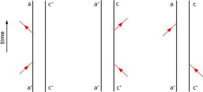
Figure 2: Double sided Feynman diagrams showing the effect of the three terms in the dynamical hybridization couplings. The red arrows represent the addition and removal of electrons from the QD respectively, and the two vertical lines represent the “ket” on the left and “bra”on the right.

From the definition (15)-(18) of the hybridization operators, and for an electrode consisting of an electron reservoir in equilibrium, we find

$$B_{ac;a^{\prime}c^{\prime}}(t)$$

$$= -D_{ac}^{-1}(t)e^{-i\omega_{ac}t}e^{i(\omega_{aa^{\prime}}-\omega_{cc^{\prime}})t}\frac{1}{\hbar^{2}}\int_{0}^{t}dt^{\prime}\int_{-\infty}^{+\infty}\frac{d\omega}{2\pi}\left[\right.$$

$$\phantom{+}\gamma_{c^{\prime}c;aa^{\prime}}(\omega,t^{\prime};t)S(\omega-\omega_{a^{\prime}a},t^{\prime})$$

$$+\gamma_{a^{\prime}a;cc^{\prime}}(\omega,t^{\prime};t)S(\omega-\omega_{c^{\prime}c},t^{\prime})$$

$$-\delta_{a^{\prime}a}\sum_{b}\lambda^{ac}_{cb;bc^{\prime}}(\omega,t^{\prime};t)S(\omega-\omega_{cb},t^{\prime})$$

$$-\delta_{c^{\prime}c}\sum_{b}\lambda^{ca}_{ab;ba^{\prime}}(\omega,t^{\prime};t)S(\omega-\omega_{ab},t^{\prime})\left.\right]$$

The derivation of this formula is provided in Appendix B, and we have defined here a function,

$$S(\omega,t) = -\frac{\sin(\omega t)}{\omega}+\frac{2i\sin^{2}[\omega\frac{t}{2}]}{\omega},$$

which accounts for the initial condition defined at a finite time, and allows us to work with Fourier transforms with respect to the initial time at $-\infty$ (see Appendix (B)). The functions $\gamma_{c^{\prime}c;aa^{\prime}}(\omega,t^{\prime};t)$ and $\lambda^{ca}_{ab;ba^{\prime}}(\omega,t^{\prime};t)$ are a generalization of the spectral functions and defined as Fourier transforms of causal response functions,

$$\gamma_{c^{\prime}c;aa^{\prime}}(\omega,t^{\prime};t) = -2\mbox{Im}\int_{-\infty}^{+\infty}dt^{\prime\prime}\Gamma_{c^{\prime}c;aa^{\prime}}(t^{\prime\prime},t^{\prime};t)e^{i\omega t^{\prime\prime}},$$

$$\lambda^{ca}_{ab;ba^{\prime}}(\omega,t^{\prime};t) = -2\mbox{Im}\int_{-\infty}^{+\infty}dt^{\prime\prime}\Lambda^{ca}_{ab;ba^{\prime}}(t^{\prime\prime},t^{\prime};t)e^{i\omega t^{\prime\prime}},$$

so that the Fourier transform integrals can extend over the entire real axis. The integrands in the previous expressions are the correlation functions appearing in (III.2); the superscript in $\Lambda$ identifies the indices on the pure dephasing operator (47), while these indices are implied by subscripts in the function $\Gamma$. The function $\Lambda$ captures the first two correlation functions in (III.2), while $\Gamma$ captures the last one, and they are defined as,

$$\Lambda^{ca}_{ab;ba^{\prime}}(t^{\prime\prime},t^{\prime};t) = -i\Theta(t^{\prime}-t^{\prime\prime})\left\langle\mathcal{T}_{0}^{ca}(t)\mathcal{T}^{ab}(t^{\prime})\mathcal{T}^{ba^{\prime}}(t^{\prime\prime})\mathfrak{R}\right\rangle,$$

$$\Gamma_{c^{\prime}c;aa^{\prime}}(t^{\prime\prime},t^{\prime};t) = -i\Theta(t^{\prime}-t^{\prime\prime})\left\langle\mathcal{T}^{c^{\prime}c}(t^{\prime})\mathcal{T}_{0}^{ca}(t)\mathcal{T}^{aa^{\prime}}(t^{\prime\prime})\mathfrak{R}\right\rangle.$$

In contrast to conventional correlation functions for a single particle propagation, these two correlation functions contain three time arguments. Their dependence on the third argument arises from the operator $\mathcal{T}^{ca}_{0}(t)$, which differs from unity only when $a\neq c$ in general. Furthermore, physically, it is only significantly different from unity when the difference between the potentials of the two states is large enough to cause significant AOC. Thus the third argument describes the shakeup of the final electrode states when the QD oscillates between two different charge states. This is fundamentally different than the processes described by the first two arguments. Specifically, the time difference $t^{\prime\prime}-t^{\prime}$ relates to the particle absorption/emission spectrum of the electrode in the presence of a QD. The average time $(t^{\prime\prime}+t^{\prime})/2$ relates to the memory of the initial state potential of the QD. In our notation, we use a semi-colon to set apart the two different kinds of time arguments.

The full mathematical analysis of correlation functions Eq. (50) is outlined in Appendix B. To gain physical insight into the results therein, we focus on the process of electron transfer from the QD to the electrodes. Then the pertinent correlation function is denoted by the superscript “>” and defined as,

$$\Gamma_{c^{\prime}c;aa^{\prime}}^{>}(t^{\prime\prime},t^{\prime};t) = \frac{-i}{Z}\Theta(t^{\prime}-t^{\prime\prime})\sum_{\nu\nu^{\prime}\boldsymbol{k}\boldsymbol{k}^{\prime}}T^{c^{\prime}c}_{\nu\boldsymbol{k}}T^{aa^{\prime}}_{\nu^{\prime}\boldsymbol{k}^{\prime}}\left\langle e^{iK_{c^{\prime}}t^{\prime}}c_{\nu\boldsymbol{k}}e^{-iK_{c}(t^{\prime}-t)}e^{iK_{a}(t^{\prime\prime}-t)}c_{\nu^{\prime}\boldsymbol{k}^{\prime}}^{\dagger}e^{-iK_{a^{\prime}}t^{\prime\prime}}e^{-\beta H_{L}}\right\rangle,$$ (51)

where we have made the physical assumption that $\mathfrak{R}=\exp(-\beta H_{L})/Z$ with the usual partition function $Z=\left<\exp(-\beta H_{L})\right>$.

The correlation function under the sum on the right hand side of (51) may be interpreted as a thermal average of overlaps between two electrode states evolving under different potentials. To see this, take a many body electrode state with $N$ electrons, $\left|\Phi(N)\right\rangle$, which would appear as a ket when computing the expectation values in (51). First consider the case where $\mathcal{T}_{0}^{ca}(t)\approx 1$, which occurs when the states $\left|a\right\rangle$ and $\left|c\right\rangle$ have the same charge. Then all the correlation functions above reduce to functions with two essential time arguments. The state $\left|\Phi(N)\right>$ initially evolves under the potential $\hat{V}_{a^{\prime}a^{\prime}}$ until time $t^{\prime\prime}$, and at this time an electron is injected from the QD into a single particle state of the electrode with in-plane momentum $\boldsymbol{k}^{\prime}$. Within this scenario, the QD can either be in a negatively charged state or in an exciton state immediately before $t^{\prime\prime}$; it cannot be in the ground state. After tunneling, the QD potential switches to $\hat{V}_{aa}$ and the state is evolved back to the initial time ($t=0$). Let us call this state $\left|\Phi^{\prime\prime}(N+1)\right\rangle$ to denote the fact that the state corresponds to time $t^{\prime\prime}$. Similarly, the bra form of $\left|\Phi(N)\right\rangle$ evolves under $\hat{V}_{c^{\prime}c^{\prime}}$ until time $t^{\prime}$, when an electron is added to it in the single particle level $\boldsymbol{k}$, and the resulting $N+1$ electron state is evolved back to the initial time under the influence of the QD potential $\hat{V}_{cc}$. We label the resulting state $\left|\Phi^{\prime}(N+1)\right\rangle$.

With these definitions, we see that the correlation function in (52) is equal to the overlap $\left\langle\Phi^{\prime}(N+1)\left|\right.\Phi^{\prime\prime}(N+1)\right\rangle$, the trace in that expression being a thermal average over all the many body states, and the summation over $\boldsymbol{k}$ and $\boldsymbol{k}^{\prime}$ is a summation over all possible in-plane momenta into which the electron can be injected. The weights for the latter summation are the tunneling amplitudes, which give the probability of such an injection to occur. We may interpret in the same way the correlation functions in which $c_{\boldsymbol{k}^{\prime}}^{\dagger}$ is to the left of $c_{\boldsymbol{k}}$. As they describe the evolution with an electron removed from the initial state, the overlap is $\left\langle\Phi^{\prime}(N-1)\left|\right.\Phi^{\prime\prime}(N-1)\right\rangle$.

It is now clear that if $\hat{V}_{c^{\prime}c^{\prime}}$ and $\hat{V}_{a^{\prime}a^{\prime}}$ are weak (for example, if their source has a vanishing charge), the propagation of $\left|\Phi(N)\right\rangle$ until the time of adding the electron is identical in both $\left|\Phi^{\prime}(N+1)\right\rangle$ and $\left|\Phi^{\prime\prime}(N+1)\right\rangle$. Therefore, the origin of time loses significance and the resulting correlation becomes a function only of the time difference $t^{\prime}-t^{\prime\prime}$. It thus reduces to a correlation function for a system in equilibrium or in a steady state, where the effects of initial conditions have decayed. Therefore, the dependence of the generalized spectral functions on $t^{\prime}$ in (III.2) is in proportion to the memory of the QD potential in the initial state. Similarly, it follows from (LABEL:eq:Lambda-Gamma) that the dependence on $t$ is in proportion to the difference between potentials of the superimposed final states at time $t$.

It follows from above that if only the monopole contribution is significant, the correlation function would depend only on the time difference, $t^{\prime}-t^{\prime\prime}$ so long as the initial and final state of the QD have the same charge. The Fourier transform of the correlation function with respect to this time difference then defines a conventional spectral function describing single particle absorption or emission as a function of energy. When coupling to the dipole and higher order potentials is strong enough, coherent oscillation between the states of different multipoles would, in general, lead to this spectral function evolving as a function of the average time $(t^{\prime}+t^{\prime\prime})/2$, thus exhibiting non-Markovian behavior.

We now summarize the mathematical expressions that can be evaluated with our physical model. In particular, we specialize to the case of quadratic Hamiltonians, and follow Blankenbecler et al (Blankenbecler et al., 1981) and Hirsch (Hirsch, 1985) to develop explicit expressions for these correlation functions in terms of a matrix inverse and matrix multiplication in the single particle basis for the electrode states. Thus for the correlation function in which an electron tunnels from the QD to the electrode, the analysis presented in Appendix B yields,

$$\Gamma_{c^{\prime}c;aa^{\prime}}^{>}(t^{\prime\prime},t^{\prime};t)=$$ (52)

$$-i\Theta(t^{\prime}-t^{\prime\prime})r_{c^{\prime}c;aa^{\prime}}(t^{\prime\prime},t^{\prime},t)\sum_{\nu,\nu^{\prime}\boldsymbol{k}\boldsymbol{k}^{\prime}}T^{c^{\prime}c}_{\nu\boldsymbol{k}}T^{aa^{\prime}}_{\nu^{\prime}\boldsymbol{k}^{\prime}}$$

$$\left\langle\nu\boldsymbol{k}\right|\mathbf{\bar{N}}_{c^{\prime}c^{\prime}}(-t^{\prime},0)\left[\mathbf{I}+\boldsymbol{\Sigma}^{(1)ca}_{c^{\prime}c;aa^{\prime}}(t^{\prime},t^{\prime\prime};t)\mathbf{\bar{N}}_{c^{\prime}c^{\prime}}(-t^{\prime},0)\right]^{-1}$$

$$\left[e^{-iK_{c^{\prime}}t^{\prime}}e^{iK_{a^{\prime}}t^{\prime\prime}}\right]\left|\nu^{\prime}\boldsymbol{k}^{\prime}\right\rangle,$$

and

$$\Lambda^{>ca}_{ab;ba^{\prime}}(t^{\prime\prime},t^{\prime};t)=$$ (53)

$$-i\Theta(t^{\prime}-t^{\prime\prime})r_{ca;ba^{\prime}}(t,t^{\prime\prime},t^{\prime})\sum_{\nu,\nu^{\prime}\boldsymbol{k}\boldsymbol{k}^{\prime}}T^{ab}_{\nu\boldsymbol{k}}T^{ba^{\prime}}_{\nu^{\prime}\boldsymbol{k}^{\prime}}$$

$$\left\langle\nu\boldsymbol{k}\right|\mathbf{\bar{N}}_{ac}(t-t^{\prime},-t)\left[\mathbf{I}+\boldsymbol{\Sigma}^{(2)ac}_{ab;ba^{\prime}}(t^{\prime},t^{\prime\prime};t)\mathbf{\bar{N}}_{ac}(t-t^{\prime},-t)\right]^{-1}$$

$$\left[e^{-iK_{c^{\prime}}t^{\prime}}e^{iK_{a^{\prime}}t^{\prime\prime}}\right]\left|\nu^{\prime}\boldsymbol{k}^{\prime}\right\rangle.$$

The superscript “>” in these definitions indicates that the correlation functions correspond to the propagation of a state in which an electron is added to the electrode (see Appendix B). The pairs of indices on the correlation function are constrained by the type of correlation function, “lesser” and “greater”, in accordance with (90).

In these expressions, the evaluation of the correlation functions has been divided into two parts. First, we have defined a more general function to capture the AOC effects for four potentials,

$$r_{c^{\prime}c;aa^{\prime}}(t^{\prime\prime},t^{\prime};t)$$

$$= \frac{1}{Z}\left\langle e^{iK_{c^{\prime}}t^{\prime}}e^{-iK_{c}(t^{\prime}-t)}e^{iK_{a}(t^{\prime\prime}-t)}e^{-iK_{a^{\prime}}t^{\prime\prime}}e^{-\beta H_{L}}\right\rangle.$$

Second, the part that explicitly depends on the hybridization functions is now reduced to the proper combination of matrices that represent each indicated operator in the natural single particle basis for the electrodes, $\left|\nu\boldsymbol{k}\right>$. The matrix $\mathbf{\bar{N}}_{ac}(t,\tau)$ is defined to be,

$$\mathbf{\bar{N}}_{ac}(t,\tau)\equiv e^{-iK_{a}t}e^{-iK_{c}\tau}\left[1+e^{-\beta H_{L}}\right]^{-1}e^{iK_{c}\tau}e^{iK_{a}t},$$ (55)

In the $\left|\nu\boldsymbol{k}\right>$ basis, the central term is simply the statistical weight for empty states

$$\frac{\delta_{\nu\boldsymbol{k},\nu^{\prime}\boldsymbol{k}^{\prime}}}{1+\exp\left\{-\left(E_{\nu\boldsymbol{k}}-\mu\right)/k_{B}T\right\}}.$$ (56)

Thus, the process for electron transfer into the electrode is proportional to the empty states available. However, the $\mathbf{\bar{N}}_{ac}(t,\tau)$ includes the time-dependent shake-up processes induced by the potential of the QD states $\left|a\right\rangle$ and $\left|c\right\rangle$. In turn, this influences the distribution of states available to receive the electron, opening additional states below or blocking states above the Fermi level.

The matrices $\boldsymbol{\Sigma}^{(j)}$, $j=1,2$, in (52) and (53) are common to both emission and absorption, and are defined as,

$$\boldsymbol{\Sigma}^{(1)bb^{\prime}}_{c^{\prime}c;aa^{\prime}}(t^{\prime},t^{\prime\prime};t) = e^{-iK_{c^{\prime}}t^{\prime}}e^{iK_{a^{\prime}}t^{\prime\prime}}e^{-iK_{a}t^{\prime\prime}}\mathcal{T}_{0}^{bb^{\prime}}(t)e^{iK_{c}t^{\prime}}-\mathbf{I},$$

$$\boldsymbol{\Sigma}^{(2)bb^{\prime}}_{c^{\prime}c;aa^{\prime}}(t^{\prime},t^{\prime\prime};t) = e^{-iK_{c^{\prime}}t^{\prime}}\mathcal{T}_{0}^{bb^{\prime}}(t)e^{iK_{a^{\prime}}t^{\prime\prime}}e^{-iK_{a}t^{\prime\prime}}e^{iK_{c}t^{\prime}}-\mathbf{I}.$$

For the correlation corresponding to an electron tunneling from the electrode to the QD, expressions similar to (52) and (53) exist (see Eqs. 95 and 97). In those correlation functions, $\mathbf{\bar{N}}$ is replaced by the compliment, $\mathbf{N}=\mathbf{I}-\mathbf{\bar{N}}$.

III.3 Energy transfer rates

We now turn to the expression for the matrices $\mathbf{P}(t)$ and $\mathbf{C}(t)$, which are the first and the second order terms, respectively, that enter in the cumulant expansion of the propagator (III.1.1). The first order term deriving from the Coulomb interaction, Eq. (40), and specialized to the Fermionic reservoir, reads

$$P_{ac;a^{\prime}c^{\prime}}(t)=-iD_{ac}^{-1}(t)\frac{e^{-i\omega_{ac}t}}{\hbar}\int_{0}^{t}dt^{\prime}$$

$$\left[\delta_{cc^{\prime}}\left\langle\mathcal{T}_{0}^{ca}(t)\hat{V}_{aa^{\prime}}(t^{\prime})\mathfrak{R}\right\rangle e^{-i\omega_{aa^{\prime}}t^{\prime}}\right.$$

$$\left.-\delta_{aa^{\prime}}\left\langle\hat{V}_{c^{\prime}c}(t^{\prime})\mathcal{T}_{0}^{ca}(t)\mathfrak{R}\right\rangle e^{-i\omega_{c^{\prime}c}t^{\prime}}\right].$$ (59)

Recall that the diagonal terms (e.g. $\hat{V}_{aa}$) do not appear in the $\hat{V}_{C}$ operator, having been put in $H_{0}$. As shown in (98) the above expression for $P_{ac;a^{\prime}c^{\prime}}$ may be expressed in terms of a Hartree energy matrix,

$$\Delta_{aa^{\prime}}(\tau)=(1-\delta_{aa^{\prime}})\langle\hat{V}_{aa^{\prime}}\mathfrak{R}^{(aa^{\prime})}(\tau)\rangle,$$ (60)

the time-dependence of which arises from the evolution of the electrode state under the influence of the average of the potentials of the QD states $\left|a\right\rangle$ and $\left|a^{\prime}\right\rangle$, which we write as

$$\mathfrak{R}^{(aa^{\prime})}(t)\equiv e^{i\frac{t}{2}(K_{a}+K_{a^{\prime}})}\mathfrak{R}e^{-i\frac{t}{2}(K_{a}+K_{a^{\prime}})}.$$

By writing the time-dependence in this manner, we fully capture the monopole contributions to pure dephasing (see Appendix B.2). The effects of first and higher moments of this density can be ignored due to the Friedel sum rule(Mahan, 2000), and have been verified by our calculations to be small. We remark that this approximation is a direct consequence of the charge conservation implied by the off-diagonal components of the Coulomb matrix in (19). Furthermore, the Hartree correction arises only in the coupling of coherences to each other and to populations due to the fact that it is of first order and that the diagonal elements of its underlying Coulomb potential matrix have been removed.

We now turn to the second order term, denoted by the matrix $\mathbf{C}(t)$, which generates energy transfer between the electrode and the QD. The full expression for $\mathbf{C}(t)$ is identical in form to that for $\mathbf{B}$, except for the appearance of the Coulomb interaction operators $\hat{V}_{ac}(t)$ instead of the hybridization operators $\mathcal{T}_{ac}(t)$. However, instead of starting with the full form, we derive the expression for $\mathbf{C}$ by neglecting the effects of AOC altogether . These effects can occur only at third order in the Coulomb interaction between the QD and the electrode. Furthermore, retaining these effects amounts to calculating the dielectric function of an electrode driven out of equilibrium by the fluctuations in the QD potential. We expect this to be a very weak effect due to the screening of this potential, and the macroscopic size of the electrode. Furthermore, since the Coulomb interaction does not change the charge of the QD states, changes in the potential induced by Coulomb processes are much weaker than hybridization. The neglect of AOC in energy transfer simplifies the expression for $\mathbf{P}_{C}(t)$ by reducing it to $\dot{\mathbf{P}}_{C}(t)=\left\langle\mathcal{J}_{C}(t)\right\rangle_{L}$. This also allows us to write the combination $\mathbf{C}-\mathbf{P}^{2}/2$ in (III.1.1) in terms of the fluctuation of potentials around their average values, with (LABEL:eq:C_gen) giving the general expression for $\mathbf{C}(t)$

Thus for states $\left|a\right\rangle$ and $\left|a^{\prime}\right\rangle$ carrying an equal charge, and $\left|c^{\prime}\right\rangle$ and $\left|c\right\rangle$ carrying an equal but not necessarily the same charge as $\left|a\right\rangle$, we obtain,

$$C_{ac;a^{\prime}c^{\prime}}(t)$$

$$= -\frac{1}{\hbar^{2}}e^{-i\omega_{ac}t}\int_{0}^{t}dt_{1}\int_{0}^{t_{1}}dt_{2}\left[\sum_{b}\right.$$

$$\phantom{+}\delta_{c^{\prime}c}\left\langle\Delta\hat{V}_{ab}(t_{1})\Delta\hat{V}_{ba^{\prime}}(t_{2})\mathfrak{R}\right\rangle e^{i(\omega_{ab}t_{1}+\omega_{ba^{\prime}}t_{2})}$$

$$\left.+\delta_{aa^{\prime}}\left\langle\Delta\hat{V}_{c^{\prime}b}(t_{2})\Delta\hat{V}_{bc}(t_{1})\mathfrak{R}\right\rangle e^{i(\omega_{bc}t_{1}+\omega_{c^{\prime}b}t_{2})}\right]$$

$$-\frac{1}{\hbar^{2}}\int_{0}^{t}dt_{1}\int_{0}^{t}dt_{2}$$

$$\left\langle\Delta\hat{V}_{c^{\prime}c}(t_{2})\Delta\hat{V}_{aa^{\prime}}(t_{1})\mathfrak{R}\right\rangle e^{i(\omega_{aa^{\prime}}t_{1}+\omega_{c^{\prime}c}t_{2})}.$$

The three terms in this expression act on the density matrix in a way similar to the corresponding three terms of the tunneling process. Here we have defined the operator for the fluctuation of $\hat{V}_{ab}$ around its mean value as,

$$\Delta\hat{V}_{ab}(t) = e^{iH_{L}t/\hbar}\hat{V}_{ab}e^{-iH_{L}t/\hbar}-\left\langle\hat{V}_{ab}\mathfrak{R}\right\rangle.$$

Note that we have neglected the effects of AOC due to the QD potential already in this definition; the subscripts on these operators only identify the matrix elements when (20) is substituted for performing calculations. We remark that the matrix elements $C_{ac;a^{\prime}c^{\prime}}(t)$ also obey the sum rule analogous to (48)

$$C_{mm;mm}(t) = -\sum_{n\neq m}C_{nn;mm}(t).$$ (62)

Following the derivation of $\gamma_{c^{\prime}c;aa^{\prime}}(\omega,t^{\prime};t)$ above, we now define the functions

$$\chi_{c^{\prime}c;aa^{\prime}}(\omega) = -2\mbox{Im}\left(1-\delta_{c^{\prime}c}\right)\left(1-\delta_{a^{\prime}a}\right)\sum_{\boldsymbol{q}}$$

$$V_{c^{\prime},\nu;c,\nu^{\prime}}(-\boldsymbol{q})X_{\nu\nu^{\prime};\mu\mu^{\prime}}(\boldsymbol{q},\omega)V_{a,\mu;a^{\prime},\mu^{\prime}}(\boldsymbol{q}),$$

where $X_{\nu\nu^{\prime};\mu\mu^{\prime}}(\boldsymbol{q},\omega)$ is the renormalized density-density correlation function, which is generalized to include inter-subband transitions. By renormalization, we mean that a summation over an infinite series of particle-hole excitations is performed between the times of the two interactions. Thus if $X_{\nu\nu^{\prime};\mu\mu^{\prime}}^{0}(\boldsymbol{q},\omega)$ is the response function of a non-interacting gas, and corresponds to a single particle-hole excitation, then

$$X_{\nu\nu^{\prime};\mu\mu^{\prime}}(\boldsymbol{q},\omega) = X_{\nu\nu^{\prime};\alpha\alpha^{\prime}}^{0}(\boldsymbol{q},\omega)$$

$$- X_{\nu\nu^{\prime};\alpha\alpha^{\prime}}^{0}(\boldsymbol{q},\omega)\mathcal{V}_{\alpha\alpha^{\prime};\beta\beta^{\prime}}(\boldsymbol{q})X_{\beta\beta^{\prime};\alpha\alpha^{\prime}}(\boldsymbol{q},\omega),$$

where $\mathcal{V}_{\alpha\alpha^{\prime};\beta\beta^{\prime}}(\boldsymbol{q})$ is the effective Coulomb interaction describing the momentum exchange $\boldsymbol{q}$ between particles scattering from bands $\alpha^{\prime},\beta^{\prime}$ and into the bands $\alpha,\beta$. This matrix is an effective interaction because it accounts for the static screening by the bulk substrate beneath the surface. When this substrate is a metal, the large plasmon frequency ensures that the bulk response may be considered instantaneous, which creates a static screening of the Coulomb potential of a surface electron, and the result defines the two-particle interaction for the surface modes. Similarly, the effective bulk dielectric function is also static for insulators or wide-gap semiconductors. The dynamical screening by the bulk may be important only for narrow-gap materials.

Following the mathematical steps outlined in Appendix B we obtain,

$$\frac{d}{dt}C_{ac;a^{\prime}c^{\prime}}(t)$$

$$= \frac{1}{2\hbar^{2}}e^{-i\omega_{ac}t}e^{i(\omega_{aa^{\prime}}-\omega_{cc^{\prime}})t}\int_{-\infty}^{+\infty}d\omega$$

$$\phantom{+}\chi_{c^{\prime}c;aa^{\prime}}(\omega)S(\omega-\omega_{cc^{\prime}},t)$$

$$+\chi_{a^{\prime}a;cc^{\prime}}(\omega)S(\omega-\omega_{aa^{\prime}},t)$$

$$-\delta_{a^{\prime}a}\sum_{b}\chi_{c^{\prime}b;bc}(\omega)S(\omega-\omega_{bc^{\prime}},t)$$

$$-\delta_{c^{\prime}c}\sum_{b}\chi_{a^{\prime}b;ba}(\omega)S(\omega-\omega_{ba^{\prime}},t).$$

This expression forms the basis of our calculations of energy transfer driven by Coulomb interaction between the QD and the electrode. We remark that the electron susceptibility in this expression may be calculated to any level of sophistication within the computational constraints. Note that we did not include electron-electron interaction within the electrode explicitly in the Hamiltonian (11). These interactions enter our theory via the correlation functions, which depend on elementary excitations that transfer energy between the electrode and the QD. Thus they can instead be taken into account fully by constructing appropriate dynamical dielectric functions and single particle Green functions.

The analysis presented so far applies only to the intrinsic couplings in the system, which lead the sub-systems to mutual equilibrium. The radiative interactions that drive these sub-systems out of equilibrium can be considered with the additional light-matter coupling shown in (23)-(II). The full development of optical response of these systems can be developed based on the above formalism. By computing the linear and non-linear optical response of surface coupled quantum dots in this way, one can develop ways in which advanced spectroscopic techniques can yield experimental measurements of the sub-system couplings. However, this is beyond the scope of the present paper.

IV Application

We now apply our model to the system shown schematically in Fig. 1 in the beginning of the paper. The goal of this section is to illustrate the calculations of the main quantitites in the formalism in the order it has been presented above. We first calculate the microscopic Hamiltonian from a model of InAs QD, and an ab-initio model of a Au[111] electrode. We use the electronic states computed from these models to obtain couplings between the subsystems. We then illustrate the use of the results of these calculations as input to our dynamical theory. In particular, we calculate the charge and energy transfer rates, and the non-radiative exciton recombination rates. In these calculations, we show the impact of FES and image effects on the dynamical charge and energy transfer couplings.

IV.1 Quantum Dot states

The QD is modeled as a dielectric sphere of InAs with radius, $a=2.0$ nm, and dielectric constant $\epsilon_{QD}=15.0$. We set the distance between the QD center and the image plane of the electrode as $h/2=2.625\;$nm. Following Chulkovet al.(Chulkov et al., 1999) we set the location of the image plane plane to be 2 Å above the top atomic layer of the electrode. To model the QD states, we use the effective mass approximation, in which we include only the lowest conduction and heavy-hole bands of bulk InAs. Thus we use (7) in the form

$$\left[-\frac{\hbar^{2}}{2m_{0}}\nabla\cdot\frac{1}{m_{j}(\boldsymbol{r})}\nabla+V(\boldsymbol{r})+\Sigma(\boldsymbol{r})-\varepsilon_{n}\right]\varphi_{n}(\boldsymbol{r})=0,$$ (66)

where $m_{j}$ is piecewise continuous with $m_{j}=1$ in the space between the QD and the electrode. Inside the geometric boundary of the QD, it is equal to the effective mass of the conduction band or a heavy-hole band for electron ($j=e$), or hole ($j=h$) states respectively. Inside the QD, we set $m_{e}=0.03$, and account for the anisotropy of the InAs heavy hole bands by setting $m_{h}=0.52$ parallel to the electrode surface and $m_{h}=0.33$ perpendicular to it. Note that this type of modeling implicitly sets the smallest spatial scale to be the lattice spacing of the QD such that its boundary is a shell of zero thickness.

The potential $V(\boldsymbol{r})$ is a square well potential of a spherical QD with $V=0$ outside the QD and $V=-5.0$ eV inside. The value inside is typical of the workfunctions of semiconductor materials, and in our discussion of dynamics below, we explore how the charge transfer rates depend on the alignment of the square well potential with the Fermi level of the electrode. The self energy, $\Sigma$, describes the electrostatic reaction field due to the polarization of the electrode and the QD surfaces, thus taking into account the image effects of both surfaces. An exact calculation of this electrostatic potential is used, the details of which can be found in our recent publication Virk et al. (2012). Since our smallest spatial scale is larger than the lattice constant, we interpolate the electrostatic image potential of the QD across this width. Another essential assumption of this electrostatics calculation is the uniform dielectric constant inside the QD, which is well-justified by several ab-initio calculations published in recent years (Wang and Zunger, 1996; Moreels et al., 2010).

Using cylindrical symmetry, we reduce the problem to two spatial dimensions, normal and parallel to the electrode surface, and solve (66) numerically over a two-dimensional grid of $(r,z)$ points using the method of finite differences. We use the the so-called ghost fluid method Liu et al. (2000) to subsume the mass discontinuity Virk et al. (2012).

Our calculated total potential for the electron in the geometry described above is shown in Fig. 3. We see from this figure that the image attraction by both the QD and the electrode lowers the potential significantly in the narrow tunnel junction around the surface normal passing through the QD center. This plays an important role in increasing the rate of electron tunneling. On the other hand tunneling is affected little for the states whose symmetry places a node in the wavefunction within this junction.

We calculate the exciton state by employing our exact solution for the electrostatic polarization to determine the matrix elements of the effective two-particle interaction potential, $V(\boldsymbol{r}_{e};\boldsymbol{r}_{h})$, in which a full account is taken of the interaction of a hole with the volume density of the electron, and the surface charge it induces Virk et al. (2012). We then expand $V(\boldsymbol{r}_{e};\boldsymbol{r}_{h})$ in the basis of product states lying below an energy cutoff, and increase this cutoff till the binding energy of the lowest exciton state converges to within 1 meV. The effect of electron-hole correlation on the resulting state is subtle but important. While the lowest exciton wavefunction is dominated by the product of the lowest electron and hole states, the mixing of states introduces corrections that can have noticeable effects on decay rates, as discussed below.

The right hand side panel in Fig.  3 shows the energy levels obtained after the exact diagonalization just described. The exciton level indicated on the figure is shown relative to the hole level of the QD. One may view this as representing the electron level correlated to a hole in the top valence level.

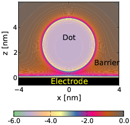
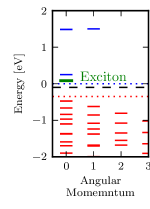
Figure 3: Left: Potential energy of an electron in the equatorial plane outside the electrode. Right: Energy levels of electron, hole and exciton states. The exciton levels is placed such that the hole of the exciton resides in the top hole level. The dashed dotted lines refer to conduction (top) and valence (bottom) band edges. The thick dashed line is the Fermi level of the electrode.

IV.2 Surface states of the electrode

To compute the electrode wavefunctions at the surface, we first perform an ab-initio calculation (using the SIESTA program Soler et al. (2002)) for bulk Au, followed by a supercell calculation with 24 mono-layers of Au oriented along the [111] direction separated by the equivalent of 36 layers of vacuum. The surface unit cell is 1x1, with no reconstruction. The TRANSIESTA Stokbro et al. (2003) code is then used to generate the Green functions for the surface Au layers via recursive decoupling Williams et al. (1982); Datta (1995) from the bulk layers. From these Green functions, we determine the projected density of states (PDOS) in which the Shockley band Shockley (1939) is identified as shown in Fig.4(a).

From the localized basis orbitals generated by SIESTA, and the eigenvectors at the poles of the surface Green function, we calculate the wavefunctions for the surface states along this band. The eigenvectors are taken along the peak of the PDOS of the surface band. Fig.4(b) shows the state at the bottom of the band superimposed on the atomic layer positions of Au[111]. Since the dispersion of this state is predominantly parabolic, its exponential decay remains essentially constant along the band. This is because the rise in total energy of a parabolic band is cancelled by the rise in its kinetic energy parallel to the surface, thereby leaving the wavenumber along the surface normal fixed to its value at the bottom of the band.

(a)

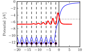
(b)

Figure 4: (a) Density of states of Au[111] surface close to the $\Gamma$ point (a). (b) The averaged potential along the surface normal. The superimposed red curve is the Shockley state. The atomic planes are indicated as dashed lines, while the image plane is shown as the solid line.

IV.3 Couplings

From these wavefunctions, and those of the QD, we determine the hybridization matrix elements $H_{T}$ from a direct application of (78). To calculate the Coulomb interaction matrix elements, we employ the procedure described by Eqs.(83-A.2). The main input to this procedure is the effective potential in which corrections due to the surface dielectric function of the electrode are applied. In order to do that, we follow Pitarke et al. Pitarke et al. (2004) and divide the surface into two linear response systems. The first is the semi-infinite bulk, and the second is the two-dimensional electron gas formed within the Shockley band. We let $\chi_{b}$ and $\chi_{s}$ be the susceptibilities of the two systems.

We define $\varepsilon^{-1}_{b}$ to be the dielectric function of the bulk, and follow Newns’ work (Newns, 1970) in calculating it. Newns’ calculation is based on the random phase approximation (RPA) within a jellium model of the electron gas, and the potential we calculate thus represents screening by the semi-infinite bulk only. Due to the large plasmon frequency of the bulk, we replace $\varepsilon_{b}$ by its static limit. We include the effects of the surface states based on the work by Pitarke et al Pitarke et al. (2004) and Silkin et al Silkin et al. (2005). In their simplified model, the surface states comprise a 2D electron gas lying in a plane a small distance $|z_{p}|$ above the interface of the semi-infinite jellium representing the bulk substrate Pitarke et al. (2004). This separation ensures charge neutrality in the interior of the jellium medium, Newns (1970) and in the present case we place the 2D plane at $z=0$, and set $z_{p}=-3\pi/8k_{F}\approx 2$Å Silkin et al. (2005).

Given $V_{0}(q,z)$ as the planar Fourier transform of a bare potential, the potential screened by the jellium plane is given by Newns (1970),

$$W(q,z) = \left[V_{0}(q,z)-V_{0}(q,z)\frac{1-\varepsilon^{-1}_{b}(q)}{1+\varepsilon^{-1}_{b}(q)}\right]\Theta(z-z_{p})$$ (67)

$$+ V_{0}(q,z_{p})\frac{2\varepsilon^{-1}(q,z-z_{p})}{\varepsilon_{b}^{-1}(q)+1}\Theta(z_{p}-z),$$

where $\varepsilon^{-1}(q,z-z_{p})$ is obtained by multiplying the pre-factor in formula (62) of Newns’ paper Newns (1970) by $-q$, and $z_{p}$ is the coordinate of the receded plane. When $V_{0}(q,z)$ corresponds to the potential of the charged QD, $W(q,z)$ enters the Hamiltonian matrix via (20) and accounts for the substrate response. The response of the surface gas appears explicitly in the dynamical rate expressions, and this asymmetry in our treatment arises because the dynamics depends only on frequencies that are much smaller than the bulk plasmon frequency. This allows us to use only the static response of the substrate, but since the surface acoustic plasmon branch extends to zero frequency, the full dynamical response of the 2D surface gas must be included. Furthermore, the coupling of the QD potential is also much larger to the electron hole excitations in the surface gas than it is in the bulk, since the potential is screened fully within a few atomic layers below the surface. The dominant coupling to surface states is also verified by the ab-initio calculation of electrode states as described above.

Thus, having made the choice to let $W(q,z)$ represent the entire bulk response, we now turn to the susceptibility $\chi_{s}$ of the 2D surface electron gas. In the present implementation approximating the general picture developed in Sec. III.3, the energy transfer rates originate from the response of the 2D electron gas. We calculate the non-interacting $\chi^{0}_{s}$ using Newns’ approach Newns (1970), and use RPA to construct the interacting response $\chi_{s}$ as in (LABEL:eq:chi-2d). In the RPA calculation, the electron-electron interaction within the 2D gas is screened by the substrate, but since the screening is only partial, collective excitations in the 2D electron gas can exist in the form of surface acoustic plasmons Pitarke et al. (2004). We find the effective screened interaction using Newns’ work,

$$v_{\mbox{\scriptsize eff}}(q)=v(q)-v(q)e^{-2q|z_{p}|}\frac{1-\varepsilon_{b}^{-1}(q)}{1+\varepsilon_{b}^{-1}(q)}.$$ (68)

Here the first term is the Fourier transform of the bare interaction within the 2D plane representing the surface electrons, and the second term is the interaction with the image charge in the substrate located in the plane a distance $2|z_{p}|$ below the surface electron plane. Substituting $v_{\mbox{\scriptsize eff}}(q)$ into the RPA summation for the 2D response, we obtain the screened susceptibility, $\chi_{s}(q,\omega)$, as

$$\chi_{s}(q,\omega)=\frac{\chi_{s}^{0}(q,\omega)}{1-v_{\mbox{{\scriptsize eff}}}(q)\chi_{s}^{0}(q,\omega)}.$$

In the left panel of Fig. 5, we have plotted a two-dimensional color map of the function $\mbox{Im}\chi_{s}(q,\omega)$ in which the bulk screening is neglected. We have verified that the acoustic plasmon branch in the absence of bulk substrate follows the expected trend, $\sqrt{e^{2}nq/(2M\varepsilon_{0})}$, which holds at low energies for a 2D gas of quasi-electrons of mass $M$ and density $n$. By including the screening due to the bulk substrate, we obtain the plot shown in the right panel. The plasmon branch in the result is significantly different as it has now acquired a linear profile that straddles along the incoherent pair continuum. Thus the bulk substrate shifts the spectral weight of the plasmon branch to a lower frequency and spreads it into the pair continuum.

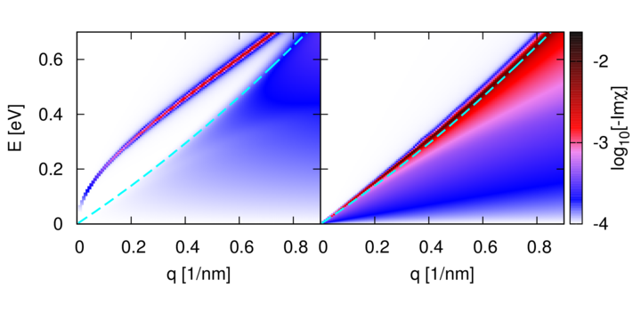
Figure 5: $\log_{10}\left[-\mbox{Im}\chi\right]$ in the absence of the semi-infinite bulk (left), and in the presence of static screening by the bulk (right). Note the qualitative change in the dispersion of the acoustic plasmon branch, which in the presence of the bulk lies close to the incoherent electron-hole continuum, the upper boundary of which is marked by the thin dashed line. Thus the spectral weight of the plasmon contributes to the pair continuum.

Let us briefly comment on when this shift can become important. Consider the processes in which a state $n$ relaxes to a lower energy state $m$ via the Coulomb interaction, in which the coupling potential is formed by the transition density $\varphi_{m}^{*}(\boldsymbol{r})\varphi_{n}(\boldsymbol{r})$. From (III.3) and energy conservation, we expect that the region in the $(q,E)$ plane that couples to this process must lie within the Fourier-Bessel transform of this potential along the $q$ axis, and in the range of energy differences $E_{n}-E_{m}$ along the $E$ axis. Wavefunctions inside a QD of radius 2 nm would generally yield the peak of the Fourier-Bessel transform to be around $q\approx 0.5\mbox{nm}^{-1}$. The plot in Fig. 5 then implies that $E_{n}-E_{m}$ must be 0.4-0.5 eV apart for the states $n$ and $m$ to experience qualitative change in their coupled dynamics. As shown by our calculations below, this energy difference is much higher than the inverse rates implied by the energy transfer matrix $\mathbf{C}(t)$ when the bulk substrate included. On the other hand, in the absence of the substrate, it is possible to approach the regime where these changes may significantly modify the time-dependence of energy transport between the QD and the electrode. We now turn to the effects of charge and energy transfer on the exciton and hole populations with the initial state in which the QD is prepared in the exciton state by photo-excitation.

IV.4 Exciton dissociation and Fermi edge singularity

In this subsection, we discuss the charge transfer of the electron to the electrode, which leaves a positively charged QD containing one hole. Since the charge state of the QD changes from neutral to positive, we expect to see the effects of the FES in the tunneling rate. With reference to the full rate expression in (III.1.1), we focus on $M_{hh;xx}$ so $D_{hh}$ and $D_{xx}$ enter, both of which are simply unity, and the rate is simply,

$$b_{x}(t)\equiv\sum_{h}\dot{B}_{hh;xx}(t).$$

A brief description of the calculation strategy is as follows. From  (III.2), we obtain

$$\dot{B}_{hh;xx}(t)=-\frac{2}{\hbar^{2}}\int_{-\infty}^{+\infty}\frac{d\omega}{2\pi}\gamma_{xh;hx}(\omega)S(\omega-\omega_{xh},t).$$ (69)

The controlling energy scale is the excess energy of the tunneling electron relative to the electrode Fermi energy, expressed by $\omega_{xh}$. We evaluate the above expression using (52), (III.2)-(LABEL:eq:sigma2). Since the dipole field of an exciton is weak and it does not affect the edge singularity by the Friedel sum rule Mahan (2000), we set $[K_{x},H_{L}]\approx 0$, which also sets $\mathbf{\bar{N}}_{xx}(t,0)\approx\mathbf{\bar{N}}$. The definition of $\gamma_{xh;hx}(\omega,t^{\prime};t)$ and this approximation together imply that it is independent of the time arguments $t^{\prime},t$, which we reflect in the equation above by omitting the time arguments (see also the discussion at the end of Sec. III.2). Taking only the surface states as the final states in the charge transfer, we obtain

$$\gamma_{xh;hx}(\omega)=-i\sum_{\boldsymbol{k}\boldsymbol{k}^{\prime}}T^{xh}_{s\boldsymbol{k}}T^{hx}_{s\boldsymbol{k}^{\prime}}\times$$ (70)

$$\int_{0}^{+\infty}d\tau e^{-i\omega\tau}r_{xh;hx}(\tau)\times$$

$$\left\langle s\boldsymbol{k}\right|\mathbf{\bar{N}}\left[\mathbf{I}+\mathbf{\Sigma}^{(1)xx}_{xh;hx}(\tau)\mathbf{\bar{N}}\right]^{-1}e^{-iK_{x}\tau}\left|s\boldsymbol{k}^{\prime}\right\rangle,$$

where $s$ denotes the surface states, and

$$r_{xh;hx}(\tau) = \frac{1}{Z}\left\langle e^{iK_{h}\tau}e^{-iK_{x}\tau}e^{-\beta H_{L}}\right\rangle,$$

$$\mathbf{\Sigma}^{(1)xx}_{xh;hx}(\tau) = e^{-iK_{x}\tau}e^{iK_{h}\tau}-\mathbf{I}.$$

Note that (70) is different from the Fermi golden rule result in that it includes the effects of sudden switching of potential to all orders in perturbation theory, and therefore includes the effects of FES exactly. This results in dressing of all operators by the Coulomb potential of the QD. The above result is a perturbation expansion with the dressed hybridization as the small parameter. Eliminating the FES effects is equivalent to setting $r_{xh;hx}(\tau)=1$, and $\mathbf{\Sigma}^{(1)xx}_{xh;hx}(\tau)=0$. Substituting these two values into (70), and performing the integral over $\tau$, the Fermi golden rule expression without the FES effects emerges in the imaginary part of $\gamma_{xh;hx}$ representing the particle loss rate from the QD.

To compute the integrand in (70), we represent $K_{a}$ in the plane-wave basis over the two-dimensional quasi-momentum within the surface band. The circular symmetry of this band reduces the problem significantly as the plane wave basis decomposes into a product of angular momentum eigenfunctions, $e^{il\theta}$, and Bessel functions $J_{l}(kr)$ for the total momentum $k$. In this basis, $K_{a}$ can be represented as a block-diagonal matrix with each block corresponding to an angular momentum eigenvalue $l$, and given by

$$\hbar K^{l}_{a;kk^{\prime}} = \frac{\hbar^{2}k^{2}}{2m_{L}}\delta_{kk^{\prime}}$$

$$+ \int_{0}^{R}dr\;r\hat{J}_{l}(kr)\hat{J}_{l}(k^{\prime}r)\int dz|\psi_{L;s}(z)|^{2}V_{aa}(r,z),$$

where $m_{L}$ is the effective mass of the surface band, $V_{aa}(r,z)$ is the potential due to the QD in state $a$ (see (37)), $|\psi_{L;s}(z)|^{2}$ is the planar averaged probability density of the surface state with negligible $k$-dependence (see Fig. 4, and Sec. IV.2), $\hat{J}_{l}(kr)$ are Bessel functions normalized to unity over $[0,R]$ such that $\hat{J}_{l}(kR)=0$, and $R$ is a cutoff radius set by discretization of $k$ and is much larger than the screening length within the two-dimensional surface electron gas. In addition, $V_{aa}(r,z)$ is constructed in accordance with the discussion in the previous section where the potential outside and inside the electrode is given by (67) respectively, and followed by Fourier transform back to real space.

We compute the resulting matrices $K^{l}_{a;kk^{\prime}}$ over a discrete set of $k$, and diagonalize them to compute their exponentials in (70), numerically exactly. Multiplying by $T^{xh}_{sk}T^{hx}_{sk^{\prime}}$ and summing over all $k,k^{\prime}$ in the discrete set, we numerically compute the integrand for a discrete set of $\tau$. By experimenting with the discretization of $k$ and the total number of angular momenta $l$, we obtained well-converged results by using $800$ $k$ points over the surface band shown in Fig. 4, and setting maximum $l$ to 24.

The resulting integrand as a function of $\tau$ generally has a slowly decaying tail that prevents a direct application of Fourier transform to obtain $\gamma(\omega)$. We follow the well-established methods to handle this numerical technicality Hawrylak (1991b, a); Mahan (1980), and then Fourier transform the resulting expression to obtain $\gamma(\omega)$. The remaining procedure to obtain $\dot{B}_{hh;xx}$ is straightforward.

In Fig. 6(a-d) we show $b_{x}(t)$ for two different alignments between the energy level of the lowest electron state and the Fermi level of the electrode. Results are also shown for two different temperatures, and plots in each figure correspond to the absence and presence of the Coulomb interaction between the QD and the electrode. We see from the figure that the tunneling rate in the presence of the interaction is always smaller than in the absence of this coupling. This effect is the result of the FES, which in turn is mainly dominated by the AOC function rather than the Mahan exciton contribution. We verified this by comparing these results with calculations in which the AOC is excluded. Decrease in the rate also results from removal of the substrate because it eliminates screening of the QD potential.

We observe in Fig. 6 that the suppression in the tunneling rate increases with temperature. This trend follows from the Anderson-Yuval mapping (Ohtaka and Tanabe, 1990), from which we expect the AOC function to exponentially decaying for time $t>\hbar/k_{B}T$ and at temperatures much smaller than the Fermi temperature of the electron gas. Since the present calculation is precisely within this regime, the suppression of rate increases with temperature. At temperatures exceeding the Fermi temperature, the orthogonality catastrophe would itself become exponentially suppressed. This regime could be reached with an electrode made of lightly doped semiconductor in which the Fermi energy can be an order of magnitude smaller. This is also the kind of system studied in an experiment by Kleemans et. al. Kleemans et al. (2010).

In addition, note from Fig. 6(b-c) that the time for $b_{x}(t)$ to reach its asymptotic value is much smaller than the inverse rate implied by its magnitude. Thus the tunneling process may be modeled accurately as Markovian with a constant rate given by $b_{x}(t)$ for $t>1\mbox{ps}$. At temperature of 10K and below, as shown in Fig. 6(a), non-Markov behavior may be expected. The longer time for the approach to asymptotic value in this regime is the result of sharp increase in the density of vacant states.

We conclude that for a semi-infinite metallic electrode, the edge singularity effect is small and quantitative, which is also in agreement with recent ab-initio work on the topic (Despoja et al., 2008). On the other hand, since the effect is proportional to the ratio of the scattering potential to the bandwidth of the Fermi sea, a lightly doped semiconductor would be a better system for its observation.

Let us briefly comment on how this crossover from the Markov to non-Markov regime may be accessible for observation. Since it occurs within the sub-picosecond timescale, the photoluminescence in this regime is completely quenched. The crossover is therefore relevant mainly to non-linear optical response of the system. A possible route to accessing this in nonlinear optics is the reduction in bleaching of exciton absorption line due to dissociation. This bleaching can be studied as a function of delay between pump pulses tuned to the absorption frequency. The rise in absorption as a function of the delay would then change from an exponential to a non-exponential function as the temperature is lowered across the crossover, which occurs at approximately 10K in the present model.

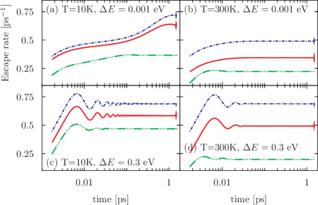
Figure 6: The escape rate of the electron in the presence of a hole with (solid red line) and without (dashed-dotted line) Coulomb coupling to the electrode. The triple-dotted green line corresponds to the rate in the absence of the bulk substrate, but with interaction with the 2D surface gas retained. Note the suppression of tunneling due to the FES. Only the lowest electron level and all the hole levels correlated to it are included. The effective junction width is 6.25 Å. Plots are shown for two different temperatures for the Fermi sea of surface states, and $\Delta E$ is the energy difference between the Fermi level and the lowest electron level. The oscillations at the rightmost end of each plot are due to the onset of aliasing as the time increases beyond the inverse of the largest energy differences imposed by the 2D momentum discretization of plane wave surface states.

IV.5 Non-radiative exciton recombination

In addition to dissociation, photoluminescence may also be quenched by non-radiative recombination (NRR) in which the energy is transferred to the electron-hole pair excitations in the electrode, rather than being converted to a photon. In the present geometry, this process is also faster than the typical radiative recombination of excitons in InAs, as we now discuss.

We first quantify the NRR of an exciton and its sensitivity to various physical properties of the system. With reference to the full rate expression in (III.1.1), we focus on $M_{gg:xx}$ so $D_{gg}$ and $D_{xx}$ enter, both of which are simply unity. Thus our theory describes this process by the matrix element $\dot{C}_{gg;xx}(t)$, which depends on $\mathbf{d}_{cv}\cdot\mathbf{E}(\boldsymbol{r})$, where $\mathbf{d}_{cv}$ is the conduction-valence band dipole matrix element at the band edge. We set its value to 2.15 Å Williamson and Zunger (1999). The vector $\mathbf{E}$ is the total electric field of the transition density of the exciton (see Appendix A),

$$\mathbf{E}(\boldsymbol{r})=-\nabla\int d\boldsymbol{s}V(\boldsymbol{r};\boldsymbol{s})\varphi_{n}(\boldsymbol{s})\varphi_{n^{\prime}}(\boldsymbol{s}),$$

where the potential $V$ also includes the electronic surface polarization response of the QD.

$$\dot{C}_{gg;xx}(t)=\frac{1}{\hbar^{2}}\sum_{\boldsymbol{q}}|V_{xg}(q)|^{2}\int_{-\infty}^{+\infty}d\omega X(q,\omega)\dot{S}(\omega-\omega_{gx},t),$$ (71)

where $X(\omega)$ is the susceptibility the computation of which we described above in Sec. IV.3, and

$$V_{xg}(q)=\mathbf{d}_{cv}\cdot\int d^{3}\boldsymbol{r}e^{-i\boldsymbol{q}\cdot\boldsymbol{r}}\mathbf{E}(\boldsymbol{r}).$$ (72)

We compute the integrand over a discrete set of $(q,\omega)$ over the range shown in Figs. 5, and sum over this range to compute $\dot{C}_{gg;xx}(t)$ at a discrete set of points $t$. The range in $q$ is sufficient due to the fact that the transition density of the exciton has a real space spread of approximately 4 nm. The range in $\omega$ is justified from the exponentially suppressed $X(q,\omega)$ above the acoustic plasmon line in Fig. 5.

In Fig. 7, we plot $\dot{C}_{gg;xx}(t)$ for various values of $l$ at which the multipole expansion of $\mathbf{E}$ is truncated. Each $l>0$ plot is therefore a correction to the often used point dipole model, in which only the $l=0$ term of the transition densities is employed. We see from the figure that the converged solution is almost twice as large as $l=0$ case, and that convergence occurs only beyond $l=3$.

As in the case of charge transfer, we may also model NRR as a Markov process with a constant rate equal to the asymptotic value of $\dot{C}_{gg;xx}(t)$. This is verified by plots of $\dot{C}_{gg;xx}(t)$ in Fig. 7, which show that after the initial appearance of an exciton state, the Fermi sea responds at the ultrafast timescale of 10 fs, within which $\dot{C}_{gg;xx}(t)$ settles to a constant value. This is much faster than the rate implied by the asymptotic value.

We remark that while NRR is almost 100 times smaller than electron tunneling rate in the figures shown, we expect from the exponential suppression of tunneling with distance, as opposed to a power law dependence of the NRR, that the non-radiative decay of an excited QD would cross over from a dissociative to a non-dissociative channel as its distance from the electrode is increased. In the present model, the tunneling rate is reduced by a factor of 10 for every extra 1.1Å of separation so that both regimes may be accessed for systems with only sub-nanometer differences in the tunnel junction. Thus the efficiency of current extraction in a photovoltaic device may be heavily impacted by NRR, and a point dipole model with uncorrelated electron-hole density suffices to estimate this impact within a factor of 2 as can be seen from Fig. 8. The correlation between the electron and the hole slightly increases the decay rate by shifting the transition density towards the metallic surface (see Fig. 9)

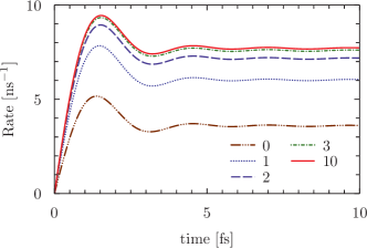
Figure 7: Forster rate calculated for increasing order $l$ (values indicated in legend) of the multipole expansion of the transition density of the exciton, including the electrostatic reaction field of the quantum dot. The oscillations result from the acoustic plasmon branch in the renormalized susceptibility of the surface electron gas.

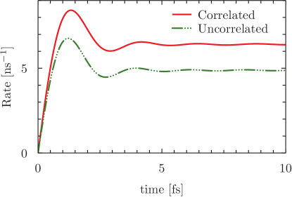
Figure 8: The Forster decay rate calculated for a product state and the fully correlated state for $l_{z}=0$. The slight increase in the Forster rate for the correlated state is the result of shift in the transition density as shown in Fig. 9.

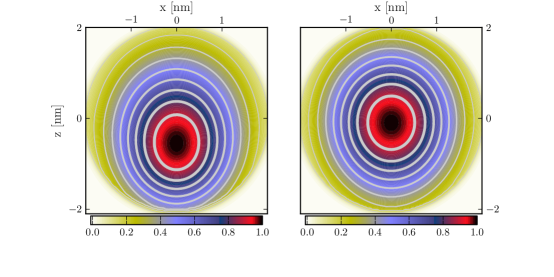
Figure 9: Contours of transition density of the fully correlated exciton state (left) compared to the charge density of the product of lowest energy electron and hole wavefunctions (right). The thickness gray contour lines represents the contour level, ranging from 1 (maximum) to 0 (minimum).

IV.6 Hole cooling and tunneling

Let us now turn to hole tunneling as well as cooling via Coulomb driven energy transfer to pair excitations. The crossover between charge and energy transfer as the dominant decay channel is also relevant here. To show this we calculate the matrix elements $\dot{B}_{gg;hh}(t)$ for tunneling, and $C_{hh;h^{\prime}h^{\prime}}(t)$ for Coulomb-driven cooling. There is a symmetry restriction in the latter so that transitions conserve the angular momentum along the surface normal of the electrode. Furthermore, due to our approximation $[K_{x},H_{L}]\approx 0$ in Sec. III.2, the computation of $\dot{B}_{gg;hh}(t)$ is obtained by replacing $x$ by $g$ in $\dot{B}_{xx;hh}(t)$. Similarly, the computation of $C_{hh;h^{\prime}h^{\prime}}(t)$ closely parallels that of $C_{gg;xx}(t)$ described in Sec. III.3. Therefore, we have omitted a discussion of computational details in this sub-section.

We plot the results of our calculations for energy transfer in the presence of a semi-infinite bulk electrode in Fig. 10. To understand the dynamical effects of bulk screening, we repeated this calculation by keeping the static image potential of the QD, but removed the screening of electron-electron interaction within the 2D gas. Thus we capture only the dynamical effects of the changes in the plasmon branch, and plot the resulting rates in Fig. 11 (the underlying loss function for this calculation is shown in left panel of Fig. 5). The reduction in the rates compared to the screened case can be understood by observing that only the points in proximity of $q\approx 0.5/nm$ and $E=0.2$ eV couple to the QD potential. This region, which lies entirely inside the incoherent pair excitation regime is farther from the plasmon branch in the absence than in the presence of the substrate screening. The resulting loss function is therefore smaller in the unscreened than in screened case. Thus the dynamical effect of screening is to enhance the rate.

However, we emphasize that the largest quantitative effect of bulk screening is to suppress this rate via the instantaneous image potential within the plane of the surface electron gas. In Fig. 12 we plot the rates when the image potential is completely removed, which corresponds to the lack of any substrate. Due to the fact that the coupling is proportional to the square of the QD potential, we see a substantial increase, by approximately a factor of 250, in the cooling rate.

We now consider these results in light of the tunneling rates of holes, plotted in Fig. 13. In the presence of the substrate, tunneling is much faster for $s$ ($l=0$) hole states, but approaches the energy transfer rates for $p$ ($l=1$) states. The much smaller tunneling rate for the $p$ state is expected from its spatial profile which contains a node in the tunnel junction. In the absence of the bulk, the energy and charge transfer rates for all states lie within factors of two to four and the two processes can thus compete. We expect this to hold true even when we account for the effect of substrate removal on tunneling.

To see why, we note that the 2D gas also generates an image potential away from its own plane, which would have the same effect on the junction potential as the image potential of a metallic substrate. The formation of this image charge may be treated as instantaneous for the purpose of tunneling, because as we have seen in the results above, the plasmon oscillations are in the regime of 10-20 fs, and the dynamical rates settle to constant values beyond this timescale. Thus the required charge re-arrangement in the 2D gas is still much faster than the tunneling rates. Also, as shown in Fig 6, the substrate removal reduces tunneling rates due to the FES, but this is still within a factor of 2. The reduced dimensionality of the electrode thus only lowers the screening of the external field within the plane of the 2D gas, and has only a small effect on the charge transfer. We conclude that tuning the substrate allows energy transfer to be controlled almost independently of charge transfer.

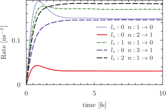
Figure 10: Cooling rates of hot holes in which energy is transferred to the electrode via the Coulomb coupling to its dynamical dielectric function. By symmetry the transfer conserves $l_{z}$, as indicated along each curve where the change in the principal quantum number $n$ is also indicated. The static screening by bulk substrate is included both in the response of the surface electron gas, and as an image correction to the field of the quantum dot.

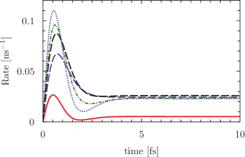
Figure 11: Cooling rates for the same states as in Fig. 10 but without the substrate induced screening of the electron-electron interaction in the surface electron gas. The reduction in the cooling rate is almost by a factor of 8, and is mainly due to the shifting of the plasmon branch up in energy or farther away from the part of loss function that couples to the transition densities. Line styles are as in Fig. 10.

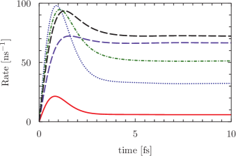
Figure 12: Cooling rates for the same states as in Fig. 10 but after completely excluding the effects of the bulk substrate. The almost 200-fold increase in the rate is due to the removal of image cancellation due to the static substrate response. A low dielectric substrate supporting a conducting thin film, such as metal-on-oxide, would correspond to this case. Line styles are as in Fig. 10.

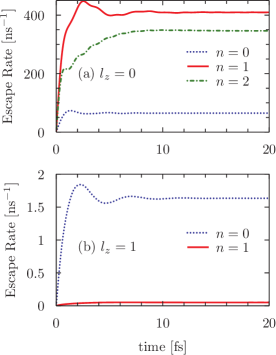
Figure 13: Rate of tunneling into a hole level of the QD with a single hole. Plots are shown for lowest energy states (principal quantum number $n$) at two different values of $l_{z}$. The charge distribution of the $l_{z}=1$ hole state is minimal near the tunnel junction, and therefore, it has a much smaller escape rate than the $l_{z}=0$ state.

V Discussion

In the previous sections, we have derived a microscopic theory and an effective model of dynamics to obtain a self-contained framework for studying surface coupled quantum dots. In this section, we discuss how the model can be applied to analyze a realistic experimental scenario, and also to analyze the experimental data. We also discuss how various physical processes, neglected here for brevity, can be described within our framework without any further modifications of the theory.

As an experiment would generally involve a collection of quantum dots spread over a region possibly much larger than their size, the charge and energy transfer rates must be averaged across the collection, and the spatial dependence of the electrode density of states. Thus both types of rates must be computed for a distribution of tunnel junction widths and changes in density of surface states across the collection of QDs. Similarly, while the optical wavelength is much larger than the size of the QD, the total optical response must also account for spatial changes in the phase of the waves across the region containing the QDs. This could be taken into account by including the factor $e^{i\boldsymbol{k}\cdot\boldsymbol{r}_{j}}$ in the optical field, where $\boldsymbol{k}$ is the wave-vector of the field and $\boldsymbol{r}_{j}$ points to the center of of the $j^{th}$ dot.

Quantum dot arrays may be designed to exploit the vast range of timescale of tunneling and the qualitative changes in exciton decay pathways, which we have demonstrated above, in order to control the transport of energy and charge across these arrays. Our theory can be extended straightforwardly to address these systems. The Hilbert space of QD states may be expanded to include electronic states of the entire array, with appropriate expansion in the size of the “system density matrix” used in our dynamical model. The Hamiltonian, $H_{D}$ would then involve both the intra-dot energy levels and inter-dot couplings, for example in a tight-binding form. The coupling to electrodes may then acquire additional dependence on QD locations, but they could still be calculated using the same methodology as outlined in this paper. Population dynamics of the density matrix of this dot array, computed in the same manner as for a single QD above, would then provide the information necessary for energy and charge transport studies.

In a similar vein, the QD density matrix may also be extended to include bi-exciton, tri-excitons, and even higher order charge complexes. The fundamental structure of our theory is a set of levels for the QD, and their dynamical coupling to the electrode. From our semi-analytical model of the surface polarization in the surface coupled QD system, the correlation energy of all higher-particle states may be determined by expanding them in product of single particle basis (though it could be impractical beyond the biexcitons). The calculation of hybridization and Coulomb interaction with the electrode then follows the same path as was used for excitons. The implications of inter-particle correlations on their Coulomb coupling to the electrode surface, and the energy transfer rates may be studied within this as was done above for exciton decay by NRR. We recall that the correlations become important when the monopole moment of the charge distribution of a state vanishes, and therefore does not set the energy scale for Coulomb coupling far above all the multipole contributions.

We have neglected vibrational levels of the QD in formulating the present theory. At the simplest level, the electron-phonon coupling within the QD provides an extra energy transfer channel for the electronic system. The discretization of vibrational levels would generally result in a non-Markovian time-dependent rate of energy exchange, which may be accounted for via a model spectral density of phonons in the QD. This would result in an extra energy transfer matrix defined in the same way as $C_{ac;a^{\prime}c^{\prime}}(t)$ in (III.3) above, the spectral function of the susceptibility in that formula replaced by the model spectral density of phonons. However, this treatment would still neglect the coherent dynamics of the electronic and the lattice system. The most extensive model would be a coupled system of electronic, photonic, and vibronic density matrices. This would allow a full study of phonons, excitons, polaritons, and photoluminescence.

VI Conclusion

In summary, we have presented a theoretical and computational framework to model the charge kinetics of optically excited quantum dots on surfaces. We have started from a microscopic construction of the eigenstates of the sub-systems, and the couplings between them, and employ them in an effective model of dynamics restricted to a small subset of these states. The model is ideally suited to explore various questions regarding the effect of the surface on charge extraction, exciton lifetime, and photoluminescence quenching in these systems. We have also developed a the dynamical theory taking into account the effects of the FES in the electrode response.

We illustrated the use of our theory by applying it to an InAs quantum dot above an Au[111] surface to which it is coupled via the Shockley surface states. Both the charge and energy transfer processes are essentially Markovian in this system, but complex dynamics may result from their interplay. We found that the FES can lower the exciton dissociation, but does so only by a factor of 2 for a Fermi sea that has a bandwidth much larger than the screened Coulomb coupling.

We also discussed the effects of multipole moments of excitons on the rate of energy transfer to the electron-hole pair excitations in the surface electron gas. The electron-hole correlation and its interplay with the image potential of the electrode has significant quantitative effects on the oscillator strength for energy loss to the plasma excitations of the electron gas. This non-radiative decay of excitons was found to be about 100 times slower than the dissociative rate for the material and geometry used in the calculations. However, with exponential scaling of the dissociative rate with the barrier width and height, and for larger QDs exhibiting greater correlation effects, competition between the two decay pathways can be expected. This would also yield rich dynamics.

Such a Coulomb driven process can also act as a cooling mechanism for a charged QD, and we have discussed in particular the cooling of holes. The energy transfer is very sensitive to the excitation spectrum at the electrode surface, and in particular the coupling of the QD to the acoustic surface plasmons. The size of the QD, and the energy level spacing, control the strength of its dynamical coupling via this mechanism, and we find that the shifting and broadening of the plasmon mode due to screening by the bulk yields a large (approximately 200-fold) reduction in the cooling rate. By arguing that this screening does not affect the formation of image potentials in the junction, we claim that screening properties of the substrate can sensitively tune this system between energy transfer and charge transfer modes of operations.

Our work can be applied to model and analyze experiments on colloidal quantum dots near semiconductor and metallic surfaces, and epitaxial quantum dots in multiple quantum wells. We have emphasized the vast range of timescales that can exist in the dynamics of these systems, and point to the various cross-overs in the dominant decay pathways for exciton states as well as the charge kinetics. In a subsequent paper, we will develop the theory of linear and non-linear optical response of these systems. Thus the excitation process itself will be studied dynamically in the presence of charge kinetics described here.

Another interesting application of this model that we have briefly discussed is the exploration of spatially dependent coupling between a quantum dot array and an electrode to control transport physics in these systems. Finally, extensions of the present theory are necessary to describe coupling to the driven vibrational modes of the quantum dot, and dynamics of photon degrees of freedom for exploring the competition between charge and energy exchange with photoluminescence and phonons. These extensions will be considered in future publications.

Appendix A Matrix elements

A.1 Hybridization

For QD states that are exponentially suppressed at the electrode surface, the hybridization may be defined by adding and subtracting $H_{L}$ to the total Hamiltonian. The decomposition has the advantage of ease of evaluation in terms of potential energy differences outside the electrode. Thus for the single electron or hole QD state we write

$$T^{ge}_{\nu\boldsymbol{k}} = \int d\boldsymbol{r}u^{*}_{\boldsymbol{k}\nu}(\boldsymbol{r})e^{-i\boldsymbol{k}\cdot\boldsymbol{r}}\left[H(\boldsymbol{r})-H_{L}(\boldsymbol{r})\right]\varphi_{e}(\boldsymbol{r}),$$ (73)

$$T^{hg}_{\nu\boldsymbol{k}} = \int d\boldsymbol{r}u^{*}_{\boldsymbol{k}\nu}(\boldsymbol{r})e^{-i\boldsymbol{k}\cdot\boldsymbol{r}}\left[H(\boldsymbol{r})-H_{L}(\boldsymbol{r})\right]\varphi_{h}(\boldsymbol{r}),$$ (74)

$$T^{eg}_{\nu\boldsymbol{k}} = T^{ge*}_{\nu\boldsymbol{k}}$$ (75)

$$T^{gh}_{\nu\boldsymbol{k}} = T^{hg*}_{\nu\boldsymbol{k}}$$ (76)

Since $\varphi_{h}$ represents a single electron orbital in the valence band, such that $\varphi_{h}^{*}$ is the state of the hole, all of the above matrix elements are defined with respect to an electron transfer. Here we have shifted the origin so that $z=0$ lies at the image plane of the electrode. The integrand vanishes on the electrode side ($z<0$), and we simplify the above formula within the effective mass approximation with a uniform mass, $m$ inside the QD. Since the kinetic energy operator acting on $\phi_{a}$ yields $E_{a}$, and the function $u_{\nu\boldsymbol{k}}(\boldsymbol{r})$ varies on a much faster scale than the rest of the functions under the integral, we obtain

$$T^{ga}_{\nu\boldsymbol{k}}=\int d\boldsymbol{r}\langle u^{*}_{\boldsymbol{k}\nu}(z)\rangle e^{-i\boldsymbol{k}\cdot\boldsymbol{r}}U_{a}(\boldsymbol{r})\varphi_{a}(\boldsymbol{r}).$$ (77)

Here we have replaced $u_{\nu\boldsymbol{k}}(\boldsymbol{r})$ by its average, $\langle u^{*}_{\boldsymbol{k}\nu}(z)\rangle$, over the planar [111] unit cell of Au lattice. Outside the electrode, $\langle u^{*}_{\boldsymbol{k}\nu}(z)\rangle$ decays exponentially, but may have additional dependence on $z$ depending on the pseudopotential in the DFT calculation. The potential energy $U_{a}$ in (77), which depends on the QD state, is defined as,

$$U_{a}(\boldsymbol{r}) = V(\boldsymbol{r})-U_{L}(\boldsymbol{r})+\left(1-\frac{m}{m_{0}}\right)\left[E_{\alpha}-V(\boldsymbol{r})\right]\Theta(\boldsymbol{r}\in\Omega_{D}).$$

Here the pseudopotential $U_{L}$ for the electrode can be extracted from the DFT calculation, the planar average of which in our calculations is shown in Fig. 4. The function $\Theta(\boldsymbol{r}\in\Omega_{D})$ is unity inside the QD and zero outside. In the presence of cylindrical symmetry, we may write the above integral in terms of a Bessel transform of order equal to the angular momentum quantum number, $l$, of the QD state,

$$T^{ag}_{\nu\boldsymbol{k}}(z) = (-1)^{l/2}\int drrU_{\alpha}(r,z)\varphi_{a}(r,z)J_{l}(kr),$$

and write,

$$T^{ag}_{\nu\boldsymbol{k}} = \int dz\left\langle u^{*}_{\boldsymbol{k}\nu}(z)\right\rangle T^{ag}_{\nu\boldsymbol{k}}(z).$$ (78)

Finally, we introduce matrix elements defining the charge transfer processes that form or dissociate an exciton state. Using the coefficients, $\Phi_{eh;x}$, for the expansion of the exciton state in terms of the electron-hole product states, we write the matrix elements for charge transfer involving an exciton state in terms of the above matrix elements connecting the ground and single particle states,

$$T^{hx}_{\nu\boldsymbol{k}} = \sum_{e}\Phi_{he;x}T^{ge}_{\nu\boldsymbol{k}},$$ (79)

$$T^{ex}_{\nu\boldsymbol{k}} = \sum_{h}\Phi_{he;x}T^{gh}_{\nu\boldsymbol{k}},$$ (80)

$$T^{xh}_{\nu\boldsymbol{k}} = T^{hx*}_{\nu\boldsymbol{k}},$$ (81)

$$T^{xe}_{\nu\boldsymbol{k}} = T^{ex*}_{\nu\boldsymbol{k}}.$$ (82)

A.2 Coulomb interaction

We write the matrix elements in (20) by separating the classical contribution,

$$V_{n,\nu\boldsymbol{k};n^{\prime},\nu^{\prime}\boldsymbol{k}^{\prime}} = W_{n,\nu\boldsymbol{k};n^{\prime},\nu^{\prime}\boldsymbol{k}^{\prime}}-\delta_{\nu\nu^{\prime}}\delta_{\boldsymbol{k},\boldsymbol{k}^{\prime}}W_{nn^{\prime}}^{(img)}.$$ (83)

In any expectation value, the subtracted term multiplies the sum over occupied states, and therefore produces $W_{nn^{\prime}}^{(img)}$ so long as the trace of the statistical matrix for the electrode is normalized to unity. The matrix elements in (83) are given by,

$$W_{n,\nu\boldsymbol{k};n^{\prime},\nu^{\prime}\boldsymbol{k}^{\prime}} = \frac{1}{2}\int d\boldsymbol{r}W_{nn^{\prime}}(\boldsymbol{r})e^{-i(\boldsymbol{k}-\boldsymbol{k}^{\prime})\cdot\boldsymbol{r}}$$

$$\times u_{\nu\boldsymbol{k}}^{*}(\boldsymbol{r})u_{\nu\boldsymbol{k}^{\prime}}(\boldsymbol{r}),$$

and

$$W_{nn^{\prime}}^{(img)} = \frac{1}{2}\int d\boldsymbol{s}\int d\boldsymbol{r}W_{nn^{\prime}}(\boldsymbol{r})\varrho_{img}(\boldsymbol{r};\boldsymbol{s}),$$

where $\varrho_{img}(\boldsymbol{r};\boldsymbol{s})$ is the charge distribution producing an image potential due to a point charge located at $\boldsymbol{s}$ outside the surface. In the above equations, $W_{nn^{\prime}}$ is the potential due of the "transitions density" of the two QD states, $\varphi_{n}(\boldsymbol{r})\varphi_{n^{\prime}}(\boldsymbol{r})$. We determine this potential from our semi-analytical solution (Virk et al., 2012) for the electrostatic potential, which yields the coefficients of multipole moments, $Q_{lm}(\boldsymbol{s})$ as a function of $\boldsymbol{s}$. Following the calculation of $Q_{lm}$ we calculate the potential of the transition density as follows. When $n$ and $n^{\prime}$ refer to the same bulk band, we exploit the fast scale of Bloch envelope functions and set their overlap to unity, and obtain

$$W_{nn^{\prime}}(\boldsymbol{r})=\sum_{l,m}\frac{1}{2\varepsilon_{0}a}\int d\boldsymbol{s}\frac{Q_{lm}(\boldsymbol{s})}{2l+1}\frac{a^{l}}{r^{l+1}}Y_{lm}(\hat{\mathbf{r}})\varphi_{n}^{*}(\boldsymbol{s})\varphi_{n^{\prime}}(\boldsymbol{s}),$$

When $n$ and $n^{\prime}$ belong to different bulk bands, the underlying Bloch envelope functions become orthogonal. In this case, we must expand the Coulomb potential over the bulk unit cell of the QD. Let $\boldsymbol{x}$ vary over the unit cell,

$$V(\boldsymbol{r}-\boldsymbol{s}-\boldsymbol{x})=V(\boldsymbol{r}-\boldsymbol{s})-\boldsymbol{x}\cdot\nabla V(\boldsymbol{r}-\boldsymbol{s}).$$

When this is averaged over the macroscopic envelope functions $\varphi_{n}(\boldsymbol{s})$, we replace $W_{nn^{\prime}}(\boldsymbol{r})$ by

$$W_{nn^{\prime}}(\boldsymbol{r})+\mathbf{d}_{nn^{\prime}}\cdot\nabla W_{nn^{\prime}}(\boldsymbol{r}),$$

where $\mathbf{d}_{nn^{\prime}}$ is the dipole moment between the Bloch states between bands $n$ and $n^{\prime}$. This is used in calculating energy transfer for exciton states in which case the zeroth order term in the field vanishes. When $\mathbf{d}_{nn^{\prime}}$ also vanishes, higher order derivatives of the potential must be coupled to the multiple moments of the microscopic Bloch functions. Replacing the overlap of Bloch envelope functions by their planar average,

$$O_{\nu\boldsymbol{k},\nu\boldsymbol{k}^{\prime}}(z)=\int d\boldsymbol{r}_{\parallel}u^{*}_{\nu\boldsymbol{k}}(\boldsymbol{r})u_{\nu\boldsymbol{k}^{\prime}}(\boldsymbol{r}),$$

we obtain,

$$W_{n,\nu\boldsymbol{k};n^{\prime},\nu^{\prime}\boldsymbol{k}^{\prime}}$$

$$= \frac{1}{2}\int dzO_{\nu\boldsymbol{k},\nu\boldsymbol{k}^{\prime}}(z)\int d\boldsymbol{r}_{\parallel}e^{i(\boldsymbol{k}^{\prime}-\boldsymbol{k})\cdot\boldsymbol{r}_{\parallel}}W_{nn^{\prime}}(\boldsymbol{r}).$$

Appendix B Charge and energy transfer rates

In this appendix, we collect the necessary mathematical steps to derive the energy and charge transfer rates as defined in (III.2) and (III.3). We make use of the equivalence of the following two expressions. Let,

$$f(t) = -i\int_{0}^{t}d\tau X(\tau)e^{i\omega_{0}\tau},$$ (86)

where $X(\tau)$ is a causal function, and the factor $i$ is for later convenience. The Fourier transform of $X(\tau)$, which is complex,

$$X(\omega)=X_{R}(\omega)+iX_{I}(\omega),$$

satisfies the Kramers-Kronig relations (Mahan, 2000). Then, we may write $f(t)$ entirely in terms of $X_{I}(\omega)$ as,

$$f(t) = \frac{1}{2}\int d\omega\mbox{Spec}\left[X(\omega)\right]S(\omega,t),$$ (87)

where we have defined the spectral function $\mbox{Spec}\left[X(\omega)\right]=-2X_{I}(\omega)$, and

$$S(\omega,t) = -\frac{\sin[(\omega-\omega_{0})t]}{\omega-\omega_{0}}+\frac{2i\sin^{2}[(\omega-\omega_{0})\frac{t}{2}]}{\omega-\omega_{0}}.$$

It is useful to note that the limiting behavior of the function $S$ is,

$$\lim_{t\rightarrow\infty}S(\omega,t) = -\pi\delta(\omega)t,$$

$$\lim_{t\rightarrow 0}S(\omega,t) = -t+i\frac{\omega t^{2}}{2}.$$

B.1 Charge transfer

The charge transfer matrix can be described by the functions defined in (LABEL:eq:Lambda-Gamma), which are explicitly equal to two of the four correlation functions in the definition of $B_{ac;a^{\prime}c^{\prime}}(t)$ in (III.2). To handle all these correlations, and to derive this reduction to two functions explicitly, we define here two additional functions,

$$\Lambda^{-ca}_{c^{\prime}b;bc}(t^{\prime\prime},t^{\prime};t) = -i\Theta(t^{\prime}-t^{\prime\prime})\left\langle\mathcal{T}^{c^{\prime}b}(t^{\prime\prime})\mathcal{T}^{bc}(t^{\prime})\mathcal{T}_{0}^{ca}(t)\mathfrak{R}\right\rangle,$$

$$\Gamma^{-}_{c^{\prime}c;aa^{\prime}}(t^{\prime\prime},t^{\prime};t) = -i\Theta(t^{\prime}-t^{\prime\prime})\left\langle\mathcal{T}^{c^{\prime}c}(t^{\prime\prime})\mathcal{T}_{0}^{ca}(t)\mathcal{T}^{aa^{\prime}}(t^{\prime})\mathfrak{R}\right\rangle.$$

It follows from the above definitions that

$$\Gamma_{c^{\prime}c;aa^{\prime}}^{-}(t^{\prime\prime},t^{\prime};t) = -\left[\Gamma_{a^{\prime}a;cc^{\prime}}(t^{\prime\prime},t^{\prime};t)\right]^{*},$$ (88)

$$\Lambda^{-ca}_{c^{\prime}b;bc}(t^{\prime\prime},t^{\prime};t) = -\left[\Lambda^{ac}_{cb;bc^{\prime}}(t^{\prime\prime},t^{\prime};t)\right]^{*},$$ (89)

Let us introduce the Fourier transforms of the correlation functions as,

$$\Gamma_{c^{\prime}c;aa^{\prime}}(\omega,t^{\prime};t) = \int_{-\infty}^{+\infty}dt^{\prime\prime}\Gamma_{c^{\prime}c;aa^{\prime}}(t^{\prime\prime},t^{\prime};t)e^{i\omega t^{\prime\prime}}.$$

The above definitions of the correlation functions and their relationship,(88) and (89) imply that

$$\mbox{Spec}\left[\Gamma_{aa^{\prime};c^{\prime}c}(\omega,t^{\prime};t)\right] = \mbox{Spec}\left[\Gamma^{-}_{cc^{\prime};a^{\prime}a}(-\omega,t^{\prime};t)\right],$$

$$\mbox{Spec}\left[\Lambda^{ca}_{aa^{\prime};c^{\prime}c}(\omega,t^{\prime};t)\right] = \mbox{Spec}\left[\Lambda^{-ac}_{cc^{\prime};a^{\prime}a}(-\omega,t^{\prime};t)\right].$$

We now use the basic relation (87), and exploit the fact that only the $\mbox{Spec}[\Gamma(\omega,t^{\prime};t)]$ and $\mbox{Spec}[\Lambda(\omega,t^{\prime};t)]$ are necessary in the final expressions. Thus performing the required permutations of states in the subscript, and setting

$$\gamma_{aa^{\prime};cc^{\prime}}(\omega,t^{\prime};t) = \mbox{Spec}\left[\Gamma_{aa^{\prime};cc^{\prime}}(\omega,t^{\prime};t)\right],$$

$$\lambda_{aa^{\prime};cc^{\prime}}(\omega,t^{\prime};t) = \mbox{Spec}\left[\Lambda_{aa^{\prime};cc^{\prime}}(\omega,t^{\prime};t)\right],$$

we obtain (III.2) in the main text. We now turn to the evaluation of these spectral functions.

The functions $\Gamma$ and $\Lambda$ can be expressed in terms of single particle Green functions of the electrode, within the interaction picture discussed in the main body. Here we explicitly develop the expressions for $\Gamma(\omega,t^{\prime};t)$, since the derivation of $\Lambda(\omega,t^{\prime};t)$ follows the same form. These Green functions are physically different depending on whether they describe propagation of the system under addition or removal of a particle. Following conventional notation we use superscript “ ^>” to describe propagation under addition of an electron to the electrode, and “^<” for the removal of an electron. Thus letting $n_{c}$ be the electron occupation of the QD in state $c$, we define

$$\Gamma_{c^{\prime}c;aa^{\prime}}(t^{\prime\prime},t^{\prime};t)=\begin{cases}\Gamma^{>}_{c^{\prime}c;aa^{\prime}}(t^{\prime\prime},t^{\prime};t)&n_{c}^{\prime}=n_{c}+1,n_{a}^{\prime}=n_{a}-1,\\ \Gamma^{<}_{c^{\prime}c;aa^{\prime}}(t^{\prime\prime},t^{\prime};t)&n_{c}^{\prime}=n_{c}-1,n_{a}^{\prime}=n_{a}+1,\end{cases}$$ (90)

where $\Gamma_{c^{\prime}c;aa^{\prime}}^{>}(t^{\prime\prime},t^{\prime};t)$ describes the tunneling of an electron out of the quantum dot and is given by (51) in the main text, while

$$\Gamma_{c^{\prime}c;aa^{\prime}}^{<}(t^{\prime\prime},t^{\prime};t) = \frac{-i}{Z}\Theta(t^{\prime}-t^{\prime\prime})\sum_{\nu\nu^{\prime}\boldsymbol{k}\boldsymbol{k}^{\prime}}T^{cc^{\prime}}_{\nu\boldsymbol{k}}T^{aa^{\prime}}_{\nu^{\prime}\boldsymbol{k}^{\prime}}\left\langle e^{iK_{c^{\prime}}t^{\prime}}c_{\nu\boldsymbol{k}}^{\dagger}e^{-iK_{c}(t^{\prime}-t)}e^{iK_{a}(t^{\prime\prime}-t)}c_{\nu^{\prime}\boldsymbol{k}^{\prime}}e^{-iK_{a^{\prime}}t^{\prime\prime}}e^{-\beta H_{L}}\right\rangle,$$ (91)

describes the tunneling from the electrode to the quantum dot. We also define $\Lambda^{\lessgtr}$ in a similar fashion to correspond to the ordering of $c^{\dagger}$ and $c$. Note that the superscripts on the hybridization matrix elements, e.g. $T^{cc^{\prime}}_{\nu\boldsymbol{k}}T^{aa^{\prime}}_{\nu\boldsymbol{k}}$ match the pairs of subscripts on the correlation function, and these pairs of indices are constrained by the type of correlation function, “lesser” or “greater”, in accordance with (90).

In the case of a quadratic Hamiltonian, this formula can be further simplified using two mathematical relations which can be proven using expressions derived by Hirsch (Hirsch, 1985). In particular, our $H_{L}$ and $K$ operators are all quadratic. The Hirsch approach allows us to connect the required full traces to the evaluation of an expression based on those operators in a single particle basis. In the following, the left hand side gives the ratio of two thermal averages while the right hand side is a specific matrix element in a single particle basis of the enclosed series of operators represented by matrices in that basis set:

$$\frac{\left\langle e^{iA_{n}x}e^{iA_{m}y}c_{i}e^{iA_{2}}c_{j}^{\dagger}e^{iA_{3}}e^{-\beta H_{L}}\right\rangle}{\left\langle e^{iA_{n}x}e^{iA_{m}y}e^{iA_{2}}e^{iA_{3}}e^{-\beta H_{L}}\right\rangle}$$ (93)

$$= \left\langle\nu\boldsymbol{k}\left|\mathbf{\bar{N}}_{mn}(-y,-x)\left[\mathbf{I}+\left(e^{-iA_{m}y}e^{-iA_{n}x}e^{-iA_{3}}e^{-iA_{2}}-\mathbf{I}\right)\mathbf{\bar{N}}_{mn}(-y,-x)\right]^{-1}e^{-iA_{m}y}e^{-iA_{n}x}e^{-iA_{3}}\right|\nu^{\prime}\boldsymbol{k}^{\prime}\right\rangle$$

$$\frac{\left\langle e^{iA_{3}}c_{i}^{\dagger}e^{iA_{2}}c_{j}e^{iA_{n}x}e^{iA_{m}y}e^{-\beta H_{L}}\right\rangle}{\left\langle e^{iA_{3}}e^{iA_{2}}e^{iA_{n}x}e^{iA_{m}y}e^{-\beta H_{L}}\right\rangle}$$

$$= \left\langle\nu\boldsymbol{k}\left|\mathbf{N}_{nm}(x,y)\left[\mathbf{I}+\left(e^{iA_{n}x}e^{iA_{m}y}e^{iA_{3}}e^{iA_{2}}-\mathbf{I}\right)\mathbf{N}_{nm}(x,y)\right]^{-1}e^{iA_{n}x}e^{iA_{m}y}e^{iA_{3}}\right|\nu^{\prime}\boldsymbol{k}^{\prime}\right\rangle.$$

In the second of the two preceding equations, $\mathbf{N}_{nm}(x,y)=\mathbf{I}-\mathbf{\bar{N}}_{nm}(x,y)$, and in the the first equation,

$$\mathbf{\bar{N}}_{mn}(y,x)=e^{iK_{m}y}e^{iK_{n}x}\left[1+e^{-\beta H_{L}}\right]^{-1}e^{-iK_{n}x}e^{-iK_{m}y},$$

where the central part is given by (56) in the main text. To apply expressions to (LABEL:eq:hirsch-1 and 93), we substitute,

$$e^{iA_{n}x}e^{iA_{m}y} = e^{iK_{c^{\prime}}t^{\prime}}=e^{iK_{c^{\prime}}t}e^{iK_{c^{\prime}}(t^{\prime}-t)},$$

$$e^{iA_{2}} = e^{-iK_{c}(t^{\prime}-t)}e^{iK_{a}(t^{\prime\prime}-t)},$$

$$e^{iA_{3}} = e^{-iK_{a^{\prime}}t^{\prime\prime}}.$$

It is also convenient to define a matrix functions,

$$\boldsymbol{\Sigma}^{(1)bb^{\prime}}_{c^{\prime}c;aa^{\prime}}(t^{\prime},t^{\prime\prime};t) = e^{-iK_{c^{\prime}}t^{\prime}}e^{iK_{a^{\prime}}t^{\prime\prime}}e^{-iK_{a}t^{\prime\prime}}\mathcal{T}_{0}^{bb^{\prime}}(t)e^{iK_{c}t^{\prime}}-\mathbf{I},$$

$$\boldsymbol{\Sigma}^{(2)bb^{\prime}}_{c^{\prime}c;aa^{\prime}}(t^{\prime},t^{\prime\prime};t) = e^{-iK_{c^{\prime}}t^{\prime}}\mathcal{T}_{0}^{bb^{\prime}}(t)e^{iK_{a^{\prime}}t^{\prime\prime}}e^{-iK_{a}t^{\prime\prime}}e^{iK_{c}t^{\prime}}-\mathbf{I},$$

and a function describing the AOC,

$$r_{c^{\prime}c;aa^{\prime}}(t^{\prime\prime},t^{\prime},t) = \left\langle e^{iK_{c^{\prime}}t^{\prime}}e^{-iK_{c}(t^{\prime}-t)}e^{iK_{a}(t^{\prime\prime}-t)}e^{-iK_{a^{\prime}}t^{\prime\prime}}e^{-\beta H_{L}}\right\rangle.$$

To apply these expressions to $\Lambda^{>ca}_{ab;ba^{\prime}}$, we substitute,

$$e^{iA_{n}x}e^{iA_{m}y} = e^{iK_{c}t}e^{iK_{a}(t^{\prime}-t)}$$

$$e^{iA_{2}} = e^{-iK_{b}t^{\prime}}e^{iK_{b}t^{\prime\prime}}$$

$$e^{iA_{3}} = e^{-iK_{a^{\prime}}t^{\prime\prime}}.$$

With these definitions, we obtain the following set of functions to describe electron and hole tunneling between the QD and the electrode,

$$\Gamma_{c^{\prime}c;aa^{\prime}}^{>}(t^{\prime\prime},t^{\prime};t)=-i\Theta(t^{\prime}-t^{\prime\prime})r_{c^{\prime}c;aa^{\prime}}(t^{\prime\prime},t^{\prime},t)$$ (94)

$$\times\sum_{\nu\nu^{\prime}\boldsymbol{k}\boldsymbol{k}^{\prime}}T^{c^{\prime}c}_{\nu\boldsymbol{k}}T^{aa^{\prime}*}_{\nu^{\prime}\boldsymbol{k}^{\prime}}\left\langle\nu\boldsymbol{k}\right|\mathbf{\bar{N}}_{c^{\prime}c^{\prime}}(-t^{\prime},0)\left[\mathbf{I}+\boldsymbol{\Sigma}^{(1)ca}_{c^{\prime}c;aa^{\prime}}(t^{\prime},t^{\prime\prime};t)\mathbf{\bar{N}}_{c^{\prime}c^{\prime}}(-t^{\prime},0)\right]^{-1}\left[e^{-iK_{c^{\prime}}t^{\prime}}e^{iK_{a^{\prime}}t^{\prime\prime}}\right]\left|\nu^{\prime}\boldsymbol{k}^{\prime}\right\rangle,$$

$$\Gamma_{c^{\prime}c;aa^{\prime}}^{<}(t^{\prime\prime},t^{\prime};t)=i\Theta(t^{\prime}-t^{\prime\prime})r_{c^{\prime}c;a^{\prime}a}(t^{\prime\prime},t^{\prime},t)$$ (95)

$$\sum_{\boldsymbol{k}\boldsymbol{k}^{\prime}}T^{aa^{\prime}}_{\nu\boldsymbol{k}}T^{c^{\prime}c}_{\nu^{\prime}\boldsymbol{k}^{\prime}}\left\langle\nu\boldsymbol{k}\right|\mathbf{N}_{c^{\prime}c^{\prime}}(t^{\prime\prime},0)\left[\mathbf{I}+\boldsymbol{\Sigma}^{(1)ca}_{a^{\prime}a;cc^{\prime}}(t^{\prime\prime},t^{\prime};t)\mathbf{N}_{c^{\prime}c^{\prime}}(t^{\prime\prime},0)\right]^{-1}\left[e^{-iK_{a^{\prime}}t^{\prime\prime}}e^{iK_{c^{\prime}}t^{\prime}}\right]\left|\nu^{\prime}\boldsymbol{k}^{\prime}\right\rangle,$$

and for $\Lambda$

$$\Lambda^{>ca}_{ab;ba^{\prime}}(t^{\prime}-t^{\prime\prime},t^{\prime};t)=-i\Theta(t^{\prime}-t^{\prime\prime})r_{ca;ba^{\prime}}(t,t^{\prime\prime},t^{\prime})$$ (96)

$$\times\sum_{\nu\nu^{\prime}\boldsymbol{k}\boldsymbol{k}^{\prime}}T^{ab}_{\nu\boldsymbol{k}}T^{ba^{\prime}}_{\nu^{\prime}\boldsymbol{k}^{\prime}}\left\langle\nu\boldsymbol{k}\right|\mathbf{\bar{N}}_{ac}(t-t^{\prime},-t)\left[\mathbf{I}+\boldsymbol{\Sigma}^{(2)ac}_{ab;ba^{\prime}}(t^{\prime},t^{\prime\prime};t)\mathbf{\bar{N}}_{ac}(t-t^{\prime},-t)\right]^{-1}\left[e^{-iK_{c^{\prime}}t^{\prime}}e^{iK_{a^{\prime}}t^{\prime\prime}}\right]\left|\boldsymbol{k}^{\prime}\nu^{\prime}\right\rangle,$$

$$\Lambda^{<ca}_{ab;ba^{\prime}}(t^{\prime}-t^{\prime\prime},t^{\prime};t)=-i\Theta(t^{\prime}-t^{\prime\prime})r_{ca;ba^{\prime}}(t,t^{\prime\prime},t^{\prime})$$ (97)

$$\times\sum_{\nu\nu^{\prime}\boldsymbol{k}\boldsymbol{k}^{\prime}}T^{ba^{\prime}}_{\nu\boldsymbol{k}}T^{ab}_{\nu^{\prime}\boldsymbol{k}^{\prime}}\left\langle\nu\boldsymbol{k}\right|\mathbf{N}_{ca}(t-t^{\prime},t)\left[\mathbf{I}+\boldsymbol{\Sigma}^{(2)ac}_{ab;ba^{\prime}}(t^{\prime},t^{\prime\prime};t)\mathbf{N}_{ca}(t-t^{\prime},t)\right]^{-1}\left[e^{iK_{c}t}e^{iK_{a}(t-t^{\prime})}e^{-iK_{a^{\prime}}t^{\prime\prime}}\right]\left|\nu^{\prime}\boldsymbol{k}^{\prime}\right\rangle.$$

B.2 Energy transfer

B.2.1 First order term

Since we are only dealing with the Coulomb term in this appendix, we will omit the subscript $C$ used in the main text for functions related to this interaction. From the definitions of the superoperators, the first order term takes the form shown in (59) in the main text. We now impose the condition that the subscripts of $\hat{V}_{ab}$ correspond to states with the same net charge, and that only the monopole terms are significant in the operators $K_{a}$. Thus we replace $K_{a}$ and $K_{a}^{\prime}$ by their average, and define the time evolution of the electrode density operator under the potential $(V_{a}+V_{a}^{\prime})/2$ as

$$\mathfrak{R}^{(aa^{\prime})}(t)=e^{i\frac{t}{2}(K_{a}+K_{a^{\prime}})}\mathfrak{R}e^{-i\frac{t}{2}(K_{a}+K_{a^{\prime}})},$$

The corrections to this are small, and quantified at the end of this discussion. The first order term now becomes,

$$\frac{d}{dt}P_{ac;a^{\prime}c^{\prime}}(t) = -iD_{ac}(t)D_{a^{\prime}c^{\prime}}^{-1}(t)\left[\frac{d}{dt}D^{-1}_{ac}(t)\int_{0}^{t}d\tau\sum_{\boldsymbol{k},\boldsymbol{k}^{\prime},\nu\nu^{\prime}}\right.$$

$$\left.\delta_{cc^{\prime}}V_{a,\nu\boldsymbol{k};a^{\prime}\nu^{\prime}\boldsymbol{k}^{\prime}}\langle c^{\dagger}_{\nu\boldsymbol{k}}c_{\nu\boldsymbol{k}^{\prime}}\mathfrak{R}^{(aa^{\prime})}(\tau)\rangle-\delta_{aa^{\prime}}V_{c^{\prime},\nu\boldsymbol{k};c,\nu^{\prime}\boldsymbol{k}^{\prime}}\langle c^{\dagger}_{\nu\boldsymbol{k}}c_{\nu\boldsymbol{k}^{\prime}}\mathfrak{R}^{(cc^{\prime})}(\tau)\rangle\right]$$

Clearly, each term under the sum is the expectation value of the potential energy as the electrode state evolves under the average potentials of the states that coupled by the off-diagonal Coulomb interaction. Thus by using our definition of the Hartree energy matrix in (60),

$$\frac{d}{dt}P_{ac;a^{\prime}c^{\prime}}(t) = -i\delta_{cc^{\prime}}D_{a^{\prime}c}^{-1}(t)\left(\Delta_{aa^{\prime}}(t)+\frac{d\log{D_{ac}(t)}}{dt}\int_{0}^{t}\Delta_{aa^{\prime}}(\tau)\right)$$ (98)

$$+i\delta_{aa^{\prime}}D_{ac^{\prime}}^{-1}(t)\left(\Delta_{c^{\prime}c}(t)+\frac{d\log{D_{ac}(t)}}{dt}\int_{0}^{t}\Delta_{c^{\prime}c}(\tau)\right)$$

To obtain the corrections beyond the above, we let $\bar{K}^{aa^{\prime}}=(K_{a}+K_{a^{\prime}})/2$, and $\delta W_{aa^{\prime}}=(\hat{V}_{aa}-\hat{V}_{a^{\prime}a^{\prime}})/2$, and write

$$\left\langle e^{-iK_{a}t}\hat{V}_{aa^{\prime}}e^{iK_{a^{\prime}}t}\mathfrak{R}\right\rangle = \left\langle\hat{V}_{aa^{\prime}}e^{i(\bar{K}^{aa^{\prime}}-\delta W_{aa^{\prime}})t}\mathfrak{R}e^{-i(\bar{K}^{aa^{\prime}}+\delta W_{aa^{\prime}})t}\right\rangle$$

$$= \left\langle\hat{V}_{aa^{\prime}}e^{it\bar{K}^{aa^{\prime}}}U_{aa^{\prime}}(t)\mathfrak{R}U^{\dagger}_{aa^{\prime}}(t)e^{-it\bar{K}^{aa^{\prime}}}\right\rangle,$$

where

$$U_{aa^{\prime}}(t)=1-i\int_{0}^{t}dt^{\prime}e^{-it\bar{K}^{aa^{\prime}}}\delta W_{aa^{\prime}}(t^{\prime})e^{it\bar{K}^{aa^{\prime}}}-\int_{0}^{t}\int_{0}^{t^{\prime}}e^{-it^{\prime}\bar{K}^{aa^{\prime}}}\delta W_{aa^{\prime}}(t^{\prime})e^{i(t^{\prime}-t^{\prime\prime})\bar{K}^{aa^{\prime}}}\delta W_{aa^{\prime}}(t^{\prime\prime})e^{it^{\prime\prime}\bar{K}^{aa^{\prime}}}+\ldots.$$

From this result, we see that the leading correction to the first order term, as approximated by (98) is given by a potential $\delta W_{aa^{\prime}}$, which is equal to the difference between two electrostatic potentials of equal charge.

B.2.2 Second order term

We derive the expression for one of the terms in the energy transfer matrix, while the remaining three terms can be computed from it. Thus let,

$$F_{ac;a^{\prime}c^{\prime}}(\tau;t) = -e^{i(\omega_{aa^{\prime}}+\omega_{c^{\prime}c})t}\times$$

$$\int_{0}^{t}d\tau\left\langle\Delta\hat{V}_{c^{\prime}c}(t-\tau)\Delta\hat{V}_{aa^{\prime}}(t)\mathfrak{R}\right\rangle e^{-i\omega_{c^{\prime}c}\tau}.$$

We define

$$\chi_{ab;b^{\prime}a^{\prime}}^{+}(\tau;t) = -i\Theta(\tau)\left\langle\Delta\hat{V}_{c^{\prime}c}(t-\tau)\Delta\hat{V}_{aa^{\prime}}(t)\mathfrak{R}\right\rangle$$

$$\chi_{ab;b^{\prime}a^{\prime}}^{-}(\tau;t) = -i\Theta(\tau)\left\langle\Delta\hat{V}_{c^{\prime}c}(t)\Delta\hat{V}_{aa^{\prime}}(t-\tau)\mathfrak{R}\right\rangle.$$

These two functions also satisfy the relation

$$\left(\chi_{c^{\prime}c;aa^{\prime}}^{+}(\tau;t)\right)^{*} = -\chi_{a^{\prime}a;c^{\prime}c}^{-}(\tau;t)$$

$$\Rightarrow\mbox{Spec}\left[\chi_{c^{\prime}c;aa^{\prime}}^{+}(\omega;t)\right] = \mbox{Spec}\left[\chi_{c^{\prime}c;aa^{\prime}}^{-}(-\omega;t)\right].$$

Using the expressions for $\Delta V$, and implying summation over repeated indices, we obtain,

$$\chi_{c^{\prime}c;aa^{\prime}}^{+}(\omega;t) = V_{c^{\prime},\nu\boldsymbol{k};c,\nu^{\prime}\boldsymbol{k}^{\prime}}V_{a,\nu\boldsymbol{p};a^{\prime},\nu^{\prime}\boldsymbol{p}^{\prime}}\times$$

$$\left[\left\langle c_{\nu\boldsymbol{k}}^{\dagger}(t-\tau)c_{\nu^{\prime}\boldsymbol{k}^{\prime}}(t-\tau)c_{\mu\boldsymbol{p}}^{\dagger}(t)c_{\mu^{\prime}\boldsymbol{p}^{\prime}}(t)\right\rangle\right.$$

$$\left.-\left\langle c_{\nu\boldsymbol{k}}^{\dagger}(t-\tau)c_{\nu^{\prime}\boldsymbol{k}^{\prime}}(t-\tau)\right\rangle\left\langle c_{\mu\boldsymbol{p}}^{\dagger}(t)c_{\mu^{\prime}\boldsymbol{p}^{\prime}}(t)\right\rangle\right].$$

In most circumstances, we may neglect defects in the electrode surfaces and assume a uniform electron gas. Within this approximation, the correlation functions must conserve momentum, and the planar Fourier transform of the QD potential also becomes a function only of the difference between the two momenta

$$V_{c^{\prime},\nu\boldsymbol{k};c,\nu^{\prime}\boldsymbol{k}^{\prime}}=V_{c^{\prime}\nu^{\prime};c\nu}(\boldsymbol{k}-\boldsymbol{k}^{\prime}) = \int V_{c^{\prime}c}(\boldsymbol{r})e^{-i(\boldsymbol{k}-\boldsymbol{k}^{\prime})\cdot\boldsymbol{r}}d\boldsymbol{r}.$$

In this case the number of momenta in the summation reduces, and we obtain

$$\chi_{c^{\prime}c;aa^{\prime}}^{+}(\omega;t) = \sum_{\boldsymbol{q}}V_{c^{\prime},\nu;c,\nu^{\prime}}(-\boldsymbol{q})X_{\nu\nu^{\prime};\mu\mu^{\prime}}(\boldsymbol{q},\omega)V_{a,\mu;a^{\prime},\mu^{\prime}}(\boldsymbol{q}).$$

Here the function, $X_{\nu\nu^{\prime};\mu\mu^{\prime}}(\boldsymbol{q},\omega)$, is the density density correlation function, generalized to include inter-subband transitions,

$$X_{\nu\nu^{\prime};\mu\mu^{\prime}}(\boldsymbol{q},\omega)=\int_{0}^{\infty}d\tau\;e^{i\omega\tau}\times$$

$$\left[\left\langle c_{\nu\boldsymbol{k}-\boldsymbol{q}}^{\dagger}(t-\tau)c_{\nu^{\prime}\boldsymbol{k}}(t-\tau)c_{\mu\boldsymbol{p}+\boldsymbol{q}}^{\dagger}(t)c_{\mu^{\prime}\boldsymbol{p}}(t)\right\rangle\right.$$

$$\left.-\left\langle c_{\nu\boldsymbol{k}}^{\dagger}(t-\tau)c_{\nu^{\prime}\boldsymbol{k}-\boldsymbol{q}}(t-\tau)\right\rangle\left\langle c_{\mu\boldsymbol{p}+\boldsymbol{q}}^{\dagger}(t)c_{\mu^{\prime}\boldsymbol{p}}(t)\right\rangle\right].$$

The calculation of density-density correlation can be found in most textbooks on solid state physics (Mahan, 2000). Substitution of these calculations into the above formula and setting $\chi=\mbox{Spec}[\chi^{+}]$ yields formula (III.3) in the main body.