Localization Method for Volume of Domain-Wall Moduli Spaces

Abstract

Volume of moduli space of non-Abelian BPS domain-walls is exactly obtained in $U(N_{c})$ gauge theory with $N_{f}$ matters. The volume of the moduli space is formulated, without an explicit metric, by a path integral under constraints on BPS equations. The path integral over fields reduces to a finite dimensional contour integral by a localization mechanism. Our volume formula satisfies a Seiberg like duality between moduli spaces of the $U(N_{c})$ and $U(N_{f}-N_{c})$ non-Abelian BPS domain-walls in a strong coupling region. We also find a T-duality between domain-walls and vortices on a cylinder. The moduli space volume of non-Abelian local ($N_{c}=N_{f}$) vortices on the cylinder agrees exactly with that on a sphere. The volume formula reveals various geometrical properties of the moduli space.

1 Introduction

A moduli space of Bogomol’nyi-Prasad-Sommerfield (BPS) solitons, which is a space of parameters describing positions, orientations and sizes, is important to understand properties of BPS solitons themselves. For example, metric of the moduli space is important to see scatterings among the BPS solitons.

Volume of the moduli space is essentially obtained from an integral of a volume form, which is constructed by the metric, over the moduli space. A local structure of the moduli space is smeared out by the volume integration, but the volume of the moduli space still has significant informations on dynamics of the BPS solitons. The volume of the moduli space is directly proportional to a thermodynamical partition function of many body system of the BPS solitons. Thermodynamics of vortices is investigated by evaluation of the volume of the moduli space Manton:1993tt ; Shah:1993us ; Manton:1998kq ; Nasir:1998kt ; Manton:2004tk .

The volume of the moduli space of the BPS solitons also tells us non-perturbative dynamics in supersymmetric gauge field theories. Nekrasov has shown that one of non-perturbative corrections in ${\mathcal{N}}=2$ supersymmetric gauge theories in four dimensions can be obtained from a volume of moduli space of self-dual Yang-Mills instantons Nekrasov:2002qd by using a localization method, developed in Moore:1997dj ; Gerasimov:2006zt . The localization method recently becomes more important to investigate the non-perturbative dynamics of supersymmetric gauge theories through exact partition functions. The exact partition function of supersymmetric gauge theory is essentially proportional to the volume of the moduli space of the BPS solitons, which produce the non-perturbative corrections.

It is very difficult to construct an explicit metric of the moduli space of the BPS solitons in generalManton:2004tk , so the calculation of the volume of the moduli space is difficult, too. However, we do not need an explicit metric on the moduli space to evaluate the volume in the localization method. This fact comes from integrability and supersymmetry behind the BPS solitons. Indeed, the supersymmetry is closely related to equivariant cohomology, which plays an important role in mathematical formulation of the localization method. Then, the localization method is very useful to calculate the volume of the moduli space and extends a range of applicable cases in the volume calculation of the BPS soliton moduli space.

The advantage of the localization method in calculating the volume has been shown in the calculation of the volume of the instanton moduli space, which gives the non-perturbative corrections in four-dimensional supersymmetric gauge theory Nekrasov:2002qd . And then, the localization method is applied to evaluate the volume of the moduli space of the non-Abelian BPS vortices Miyake:2011yr . The results from the localization method perfectly agree with the previous results using the other method, and we could extend to more complicated systems, where the metric of the moduli space is not explicitly known.

In this paper, we calculate the volume of the moduli space of the non-Abelian BPS domain-walls, which is described by first order differential equations for matrix- and vector-valued variables, where the matrices are in adjoint representations of $U(N_{c})$ and $N_{f}$ sets of the vectors are in fundamental representations of $U(N_{c})$. We consider the BPS equations of the domain-walls on a finite line interval with boundaries. Solutions of the BPS domain-wall equations depend on boundary conditions. So we need to carefully treat the boundary conditions to consider the moduli spaces of the BPS domain-walls. The differential equations of the domain-walls can be regarded as a BPS equations in supersymmetric gauge theory with $U(N_{c})$ gauge group and $N_{f}$ flavors (matters) in the fundamental representation. The domain-walls are soliton like object with co-dimension one in supersymmetric gauge theory. We are interested in the moduli space of the BPS equations only, so we do not assume an explicit supersymmetric system in the calculation of the volume.

We utilize the localization method associated with the equivariant cohomology in mathematics in order to evaluate the volume of the moduli space of the BPS domain-walls. The localization method is essentially equivalent to an evaluation of a field theoretical partition function of some constrained system. A path integral of the partition function is restricted on the moduli space of the domain-walls. We again emphasize that we need the constraints of the BPS equations, but do not need an explicit metric of the moduli space in this localization method.

The path integral which gives the volume of the moduli is localized at fixed points of a symmetry, which is a part of the supersymmetry. This symmetry is called a Becchi-Rouet-Stora-Tyutin (BRST) symmetry and related to the equivariant cohomology. In the evaluation of the path integral, it is necessary to know the number of zero modes of the fields. We find that the number of the zero modes is determined by the boundary conditions, and is given by a Callias like index theorem with boundary. After counting the zero modes explicitly, we find that the path integral reduces to a usual contour integral and a simple formula is obtained for the volume of the moduli space of the BPS domain-walls. For non-Abelian gauge theories, we find that the contour integral reduces to a sum of products of the Abelian gauge theories with non-trivial signs. The sign of each product in the sum could not be determined by the localization method itself. We assume that the signs is determined by a topological index (intersection number) of the profile of the solution. Then, the sum of products is expressed by a determinant of a simple matrix depending on the boundary conditions.

In order to check our volume formula for the moduli space of the BPS domain-walls, we discuss dualities between various systems of the domain-walls. First of all, we investigate the duality between the moduli spaces of the non-Abelian BPS domain-walls in the strong coupling (asymptotic) region. We find that the moduli spaces of the domain-walls of $U(N_{c})$ and $U(\tilde{N}_{c})$ differ from each other in general, but if $\tilde{N}_{c}$ is given by $N_{f}-N_{c}$, then we expect that the moduli spaces (and its volume) coincide with each other in the strong coupling region Isozumi:2004va ; Antoniadis:1996ra . We can conclude that our results agrees with the expected dualities. Secondly, we show that there exists a T-dual relation between the domain-walls and vortices on a cylinder Eto:2004vy . The domain-walls and vortices have different co-dimensions, but if we consider the domain-walls winding along a circle direction of the cylinder, the volume of the moduli space can be regarded as that of the moduli space of the vortices on the cylinder Eto:2007aw . The winding number of the domain-walls corresponds to a vortex charge. We find that the volume of the moduli space of the vortices on the cylinder coincides with that of the vortices on the sphere if $N_{c}=N_{f}$ (non-Abelian local vortex). These non-trivial duality relations support that our volume formula for the moduli space of the BPS domain-walls correctly works.

This paper is organized as follows: In the next section, we explain a general argument on the volume calculation of the moduli space of the BPS equations. We introduce a path integral over the constrained system to evaluate the volume without the explicit metric. In section 3, we evaluate the path integral to see that it is localized at fixed points of the BRST symmetry, and reduces to a simple contour integral. In section 4, we explicitly evaluate the contour integral for various examples of domain-walls in Abelian and non-Abelian gauge theories. In order to check our results for the volume of the moduli space of the BPS domain-walls, we consider two kinds of dualities of the moduli spaces in section 5 and 6. The last section is devoted to conclusion and discussion.

2 Volume of Moduli Space

We take the $U(N_{c})$ gauge theory with the gauge field $A_{\mu}$, together with a real scalar field $\Sigma$ in the adjoint representation and $N_{f}$ complex scalar field $H_{r}^{A},r=1,\cdots N_{c},A=1,\cdots,N_{f}$ in the fundamental representation. The gauge coupling and the Fayet-Iliopoulos (FI) parameter are denoted as $g$ and $c$, respectively. Let us consider the BPS equations for domain-walls Isozumi:2004jc ; Isozumi:2004va ; Eto:2006ng in a finite interval $y\in[-\frac{L}{2},\frac{L}{2}]$:

$$\mu_{r} \equiv {\mathcal{D}}_{y}\Sigma-\frac{g^{2}}{2}\left(c{\bf 1}_{N_{c}}-HH^{\dagger}\right)=0,$$ (2.1)

$$\mu_{c} \equiv {\mathcal{D}}_{y}H+\Sigma H-HM=0,$$ (2.2)

$$\mu_{c}^{\dagger} \equiv {\mathcal{D}}_{y}H^{\dagger}+H^{\dagger}\Sigma-MH^{\dagger}=0,$$ (2.3)

where $\Sigma$, $H$ and $H^{\dagger}$ are $N_{c}\times N_{c}$, $N_{c}\times N_{f}$ and $N_{f}\times N_{c}$ matrix-valued functions of $y$, respectively, and the covariant derivatives are defined by ${\mathcal{D}}_{y}\Sigma=\partial_{y}\Sigma+i[A_{y},\Sigma]$, ${\mathcal{D}}_{y}H=\partial_{y}H+iA_{y}H$ and ${\mathcal{D}}_{y}H^{\dagger}=\partial_{y}H^{\dagger}-iH^{\dagger}A_{y}$. The mass matrix $M$ is taken to be diagonal as $M=\operatorname{diag}(m_{1},m_{2},\ldots,m_{N_{f}})$ and ordered as $m_{1}<m_{2}<\cdots<m_{N_{f}}$ without loss of generality.

Domain-wall solutions are defined by specifying vacuum at the left and right boundaries. Vacua of the system are labeled by choosing $N_{c}$ out of $N_{f}$ flavors, Isozumi:2004jc ; Isozumi:2004va ; Eto:2006ng such as $(A_{1},\cdots,A_{N_{c}})$, with $A_{1}<A_{2}<\cdots A_{N_{c}}$. Let us consider domain-wall solutions connecting the vacuum $(A_{1},\cdots,A_{N_{c}})$ at the left boundary $y=-L/2$ and the vacuum $(B_{1},\cdots,B_{N_{c}})$ at the right boundary $y=L/2$. For finite intervals, we demand the following boundary condition at the left boundary $y=-L/2$:

$$\Sigma\left(-\frac{L}{2}\right) = \operatorname{diag}(m_{A_{1}},m_{A_{2}},\ldots,m_{A_{N_{c}}}),$$ (2.4)

$$H_{r=A_{r}}^{A} = 0,\quad A<A_{r}.$$ (2.5)

Similarly at the right boundary $y=L/2$, we demand

$$\Sigma\left(\frac{L}{2}\right) = \operatorname{diag}(m_{B_{1}},m_{B_{2}},\ldots,m_{B_{N_{c}}}),$$ (2.6)

$$H_{r=B_{r}}^{A} = 0,\quad A>B_{r}.$$ (2.7)

Since Weyl permutations are a part of gauge invariance, we need to combine possible Weyl permutations of these boundary conditions.

The BPS equations (2.1), (2.2) and (2.3) with the above boundary conditions produce soliton-like objects which are localized on the one-dimensional interval and connect field configurations specified by the label of indices $\vec{A}=(A_{1},\cdots,A_{N_{c}})$ and $\vec{B}=(B_{1},\cdots,B_{N_{c}})$. Since these BPS solitons have unit co-dimension and constructed using a non-Abelian gauge theory, these BPS solitons are called non-Abelian domain-walls.

The moduli space of domain-walls is defined by a space of parameters of solutions of the BPS equations with identification up to gauge transformations. Hence the moduli space is represented by a quotient space by the $U(N_{c})$ gauge identification

$${\mathcal{M}}^{N_{c},N_{f}}_{\vec{A}\to\vec{B}}=\frac{\mu_{r}^{-1}(0)\cap\mu_{c}^{-1}(0)\cap{\mu_{c}^{\dagger}}^{-1}(0)}{U(N_{c})},$$ (2.8)

where $\mu_{r}^{-1}(0)$, $\mu_{c}^{-1}(0)$ and ${\mu_{c}^{\dagger}}^{-1}(0)$ stand for the space of solutions of the BPS equations $\mu_{r}=\mu_{c}=\mu_{c}^{\dagger}=0$ with the boundary conditions labeled by $\vec{A}$ and $\vec{B}$ at $y=-L/2$ and $y=L/2$, respectively. This quotient space is known to be a Kähler quotient space, and $\mu_{r}$, $\mu_{c}$ and $\mu_{c}^{\dagger}$ are called moment maps in this sense.

The volume of the moduli space is usually defined by an integral of the volume form over the whole moduli space with $2n$-dimensional coordinates $x$

$${\rm Vol}\left({\mathcal{M}}^{N_{c},N_{f}}_{\vec{A}\to\vec{B}}\right)=\int_{{\mathcal{M}}^{N_{c},N_{f}}_{\vec{A}\to\vec{B}}}d^{2n}x\sqrt{\det g_{ij}},$$ (2.9)

if we know a metric of the moduli space $g_{ij}$. However it is difficult to find the metric of the moduli space explicitly in general.

To avoid a direct integration of the volume form on the moduli space, we note that the Kähler manifold admits the Kähler form $\Omega$ and the volume form on the Kähler quotient space can be written in terms of $\Omega$ as $d^{2n}x\sqrt{\det g_{ij}}=\frac{1}{n!}\Omega^{n}$. On the moduli space, the volume is expressed by

$${\rm Vol}\left({\mathcal{M}}^{N_{c},N_{f}}_{\vec{A}\to\vec{B}}\right)=\int_{{\mathcal{M}}^{N_{c},N_{f}}_{\vec{A}\to\vec{B}}}e^{\Omega},$$ (2.10)

under the consent that the integral exists only on the $2n$-form.

We can also express the volume integral (2.10) by a path integral over all field configurations with suitable constraints onto the moduli space ${\mathcal{M}}^{N_{c},N_{f}}_{\vec{A}\to\vec{B}}$

$${\rm Vol}\left({\mathcal{M}}^{N_{c},N_{f}}_{\vec{A}\to\vec{B}}\right)=\frac{1}{{\rm Vol}(\mathcal{G})}\int{\mathcal{D}}\Phi\,{\mathcal{D}}\vec{{\mathcal{B}}}_{v}\,{\mathcal{D}}\vec{{\mathcal{F}}}_{v}\,{\mathcal{D}}^{2}\vec{{\mathcal{B}}}_{m}\,{\mathcal{D}}^{2}\vec{{\mathcal{F}}}_{m}\,e^{-S_{0}},$$ (2.11)

where $\vec{{\mathcal{B}}}_{v}=(A_{y},\Sigma)$ and $\vec{{\mathcal{F}}}_{v}=(\lambda_{y},\xi)$ are vectors of bosonic and fermonic fields in the adjoint representation, $\vec{{\mathcal{B}}}_{m}=(H,Y_{c})$ and $\vec{{\mathcal{F}}}_{m}=(\psi,\chi_{c})$ are vectors of bosonic and fermonic fields in the fundamental representation, and ${\rm Vol}(\mathcal{G})$ is the volume of $U(N_{c})$ gauge transformation group $\mathcal{G}$. Precisely speaking, the definition of the volume of the moduli space via the path integral has an ambiguity corresponding to an ambiguity in the definition of the normalization of the metric (Kähler form) of the moduli space. We will discuss this point later.

We choose an “action” $S_{0}$ to give constraints on the moduli space, which are achieved by integrating over Lagrange multiplier fields $\Phi$, $Y_{c}$ and $Y_{c}^{\dagger}$, and introduce fermions $\lambda_{y}$, $\xi$, $\psi$, $\psi^{\dagger}$, $\chi_{c}$ and $\chi_{c}^{\dagger}$ to give a suitable Kähler form on the moduli space and Jacobians for the constraints. Inspired by the general discussion in Miyake:2011yr , we take the following action $S_{0}$

$$S_{0}=i\beta\int_{-\frac{L}{2}}^{\frac{L}{2}}dy\,\operatorname{Tr}\Big{[}\Phi\mu_{r}-\lambda_{y}\xi+i\frac{g^{2}}{2}\psi\psi^{\dagger}+Y_{c}^{\dagger}\mu_{c}\\ -\chi_{c}^{\dagger}\left(\frac{\delta\mu_{c}}{\delta A_{y}}\lambda_{y}+\frac{\delta\mu_{c}}{\delta\Sigma}\xi+\frac{\delta\mu_{c}}{\delta H}\psi\right)+(\text{h.c.})\Big{]},$$ (2.12)

in order to impose the constraints, and to give the Kähler form and Jacobians in the path integral over the field configurations. We also introduced a parameter $\beta$ with a dimension of length. Thus the volume of the domain-wall moduli space is evaluated by the path integral over fields like a partition function of a gauge field theory. The role of the Lagrange multiplier field $\Phi$ is rather special compared to other fields. We treat the path integral over $\Phi$ separately from other fields.

We can evaluate the integral (2.11) directly by using a usual field theoretical procedure as performed in Miyake:2011yr . However, once we noticed that the action $S_{0}$ possesses an extra symmetry (BRST symmetry), we can evaluate the path integral (2.11) via the so-called localization method (cohomological field theory) much more easily than the direct evaluation of the path integral. We will see that the path integral (2.11) is localized at the fixed point sets of the BRST symmetry and is reduced to a finite dimensional integral.

3 Localization in Field Theory

To proceed the evaluation of the path integral (2.11), we introduce the following fermionic transformations (BRST transformations) for the vector fields (fields in the adjoint representation)

$$\begin{array}[]{ll}QA_{y}=\lambda_{y},&Q\lambda_{y}=-{\mathcal{D}}_{y}\Phi,\\ Q\Sigma=\xi,&Q\xi=i[\Phi,\Sigma],\\ Q\Phi=0,\end{array}$$ (3.1)

and for the matter fields (fields in the fundamental representation)

$$\begin{array}[]{ll}QH=\psi,&Q\psi=i\Phi H,\\ QY_{c}=i\Phi\chi_{c},&Q\chi_{c}=Y_{c},\end{array}$$ (3.2)

and for their hermitian conjugates. We see a square of this transformation generates a gauge transformation $\delta_{G}(\Phi)$ with $\Phi$ as the transformation parameter: $Q^{2}=\delta_{G}(\Phi)$. This means that $Q^{2}$ is nilpotent on gauge invariant operators ${\mathcal{O}}$. If we restrict a space of operator fields to the gauge invariant ones, $Q$ gives a cohomology by an identification

$${\mathcal{O}}\sim{\mathcal{O}}+Q(\text{gauge inv.~{}op.}),$$ (3.3)

which is called the equivariant cohomology.

Under this transformation, we find that the action $S_{0}$ is invariant ($Q$-closed)

$$QS_{0}=0.$$ (3.4)

We also find that the action $S_{0}$ can be written by

$$S_{0}=i\beta\int_{-\frac{L}{2}}^{\frac{L}{2}}dy\,\operatorname{Tr}\left[\Phi\left({\mathcal{D}}_{y}\Sigma-\frac{g^{2}c}{2}{\bf 1}_{N_{c}}\right)-\lambda_{y}\xi\right]\\ +i\beta Q\int_{-\frac{L}{2}}^{\frac{L}{2}}dy\,\operatorname{Tr}\left[-\frac{g^{2}}{2}\psi H^{\dagger}+\mu_{c}\chi_{c}^{\dagger}+\chi_{c}\mu_{c}^{\dagger}\right].$$ (3.5)

Here we imposed the periodic boundary condition for the product $\Phi\xi$ in order to preserve the BRST invariance for the action. So an essential cohomological part ($Q$-closed but not $Q$-exact) of the action $S_{0}$ is

$$S_{\text{coh}}=i\beta\int_{-\frac{L}{2}}^{\frac{L}{2}}dy\,\operatorname{Tr}\left[\Phi\left({\mathcal{D}}_{y}\Sigma-\frac{g^{2}c}{2}{\bf 1}_{N_{c}}\right)-\lambda_{y}\xi\right],$$ (3.6)

in terms of the equivariant cohomology.

Using the nature of the BRST symmetry, we can add an extra $Q$-exact action $Q\Xi$ to $S_{0}$ without changing the path integral, that is, the deformed path integral

$${\rm Vol}\left({\mathcal{M}}^{N_{c},N_{f}}_{\vec{A}\to\vec{B}}\right)=\frac{1}{\mathrm{Vol}(\mathcal{G})}\int{\mathcal{D}}\Phi\,{\mathcal{D}}\vec{{\mathcal{B}}}_{v}\,{\mathcal{D}}\vec{{\mathcal{F}}}_{v}\,{\mathcal{D}}^{2}\vec{{\mathcal{B}}}_{m}\,{\mathcal{D}}^{2}\vec{{\mathcal{F}}}_{m}\,e^{-S_{0}-tQ\Xi},$$ (3.7)

is independent of a deformation parameter (coupling) $t$ since the path integral measure is constructed to be $Q$-invariant. In the $t\to 0$ limit, the path integral (3.7) reduces to the original one which gives the volume of the moduli space. When we choose the deformation parameter $t$ appropriately, we can evaluate the path integral exactly.

To evaluate the path integral, we choose $\Xi$ to be the following form

$$tQ\Xi=t_{1}Q\Xi_{1}+t_{2}Q\Xi_{2},$$ (3.8)

where

$$\Xi_{1} = \int_{-\frac{L}{2}}^{\frac{L}{2}}dy\,\operatorname{Tr}\left[\mu_{c}\chi_{c}^{\dagger}+\chi_{c}\mu_{c}^{\dagger}\right],$$ (3.9)

$$\Xi_{2} = \frac{1}{2}\int_{-\frac{L}{2}}^{\frac{L}{2}}dy\operatorname{Tr}\left[\vec{{\mathcal{F}}}_{m}\cdot(Q\vec{{\mathcal{F}}}^{\dagger}_{m})+\vec{{\mathcal{F}}}_{m}^{\dagger}\cdot(Q\vec{{\mathcal{F}}}_{m})\right].$$ (3.10)

The former $Q\Xi_{1}$ is already included in the original action $S_{0}$ and gives a $\delta$-functional constraint on $\mu_{c}=\mu_{c}^{\dagger}=0$ by integrating out the $Y_{c}$ and $Y^{\dagger}_{c}$. This constraint means that the field configuration must satisfy

$${\mathcal{D}}_{y}H+\Sigma H-HM=0,$$ (3.11)

for the bosonic field $H$. The fermionic fields in the fundamental representation must strictly obey the equation of motion

$${\mathcal{D}}_{y}\psi+\Sigma\psi-\psi M=0,$$ (3.12)

$${\mathcal{D}}_{y}\chi_{c}-\chi_{c}\Sigma+M\chi_{c}=0.$$ (3.13)

As we will see later, the above constraints for the fields in the fundamental representation are important to count the number of zero modes of the fields at the localization point.

First of all, we introduce Cartan-Weyl basis $(\mathtt{H}_{a},\mathtt{E}_{\alpha},\mathtt{E}_{-\alpha})$ of the Lie algebra $\mathfrak{u}(N_{c})$ and decompose the fields in the adjoint representation as follows:

$$\Phi = \sum_{a=1}^{N_{c}}\Phi^{a}\mathtt{H}_{a}+\sum_{\alpha>0}\Phi^{\alpha}\mathtt{E}_{\alpha}+\sum_{\alpha>0}\Phi^{-\alpha}\mathtt{E}_{-\alpha},$$ (3.14)

$$A_{y} = \sum_{a=1}^{N_{c}}A_{y}^{a}\mathtt{H}_{a}+\sum_{\alpha>0}A_{y}^{\alpha}\mathtt{E}_{\alpha}+\sum_{\alpha>0}A_{y}^{-\alpha}\mathtt{E}_{-\alpha},$$ (3.15)

$$\Sigma = \sum_{a=1}^{N_{c}}\Sigma^{a}\mathtt{H}_{a}+\sum_{\alpha>0}\Sigma^{\alpha}\mathtt{E}_{\alpha}+\sum_{\alpha>0}\Sigma^{-\alpha}\mathtt{E}_{-\alpha},$$ (3.16)

where $\mathtt{H}_{a}$, $\mathtt{E}_{\alpha}$ and $\mathtt{E}_{-\alpha}$ satisfy the following commutation relations

$$[\mathtt{H}_{a},\mathtt{H}_{b}]=0,$$ (3.17)

$$[\mathtt{H}_{a},\mathtt{E}_{\alpha}]=\alpha_{a}\mathtt{E}_{\alpha},$$ (3.18)

$$\operatorname{Tr}\mathtt{E}_{\alpha}\mathtt{E}_{\beta}=\delta_{\alpha+\beta,0},$$ (3.19)

and $\mathtt{E}_{-\alpha}=\mathtt{E}_{\alpha}^{\dagger}$.

To perform the path integral, we introduce the ghosts $c$ and $\bar{c}$ for the diagonal gauge fixing condition ($\Phi^{\alpha}=0$). The ghosts induce the action

$$S_{\text{ghost}}=i\beta\int_{-\frac{L}{2}}^{\frac{L}{2}}dy\,\operatorname{Tr}c[\Phi,\bar{c}],$$ (3.20)

which gives a one-loop determinant

$$\prod_{\alpha>0}\left(\beta\alpha(\Phi)\right)^{2f^{\text{adj}}_{\alpha}}.$$ (3.21)

where $f^{\text{adj}}_{\alpha}$ represents the degree of freedom for each off-diagonal component of real fermion in one-dimension. In this gauge choice, the bosonic term for the $Q$-closed action (3.6) can be written as

$$\left.S_{\text{coh}}\right|_{\text{bosonic}}=i\beta\int_{-\frac{L}{2}}^{\frac{L}{2}}dy\,\left[\sum_{a=1}^{N_{c}}\Phi^{a}\left(\partial_{y}\Sigma^{a}-\frac{g^{2}c}{2}\right)+i\sum_{\alpha}\alpha(\Phi)A_{y}^{-\alpha}\Sigma^{\alpha}\right].$$ (3.22)

The path integral over off-diagonal elements $(A^{\alpha}_{y},\Sigma^{\alpha})$ leads to the one-loop determinant for bosonic fields in the vector multiplet

$$\prod_{\alpha>0}|\beta\alpha(\Phi)|^{-2b^{\text{adj}}_{\alpha}}.$$ (3.23)

From (3.21) and (3.23), we obtain the one-loop determinant for off-diagonal elements in the adjoint representation

$$\prod_{\alpha>0}\frac{\left(\beta\alpha(\Phi)\right)^{2f^{\text{adj}}_{\alpha}}}{|\beta\alpha(\Phi)|^{2b^{\text{adj}}_{\alpha}}}.$$ (3.24)

Naively scalar fields and vector fields carry the same degrees of freedom in one-dimension, so we can conclude that $b^{\text{adj}}_{\alpha}=f^{\text{adj}}_{\alpha}$, that is, the one-loop determinants for the adjoint fields are canceled out up to a signature $\pm 1$. It is difficult to determine the signature of the one-loop determinant at this stage, but we will assume later that this signature depends on permutations of the boundary conditions. We can non-trivially check that this assumption is consistent and leads correct answers to the volume and dualities of the domain-walls.

Next we evaluate the one-loop determinant of the fields in the fundamental representation. The matter fields enter in the action through the $Q$-exact term;

$$Q\Xi_{2} = \int_{-\frac{L}{2}}^{\frac{L}{2}}dy\left[i\sum_{a=1}^{N_{c}}(H^{\dagger}_{a}\Phi^{a}H_{a}+\chi^{\dagger}_{c,a}\Phi^{a}\chi_{c,a})+i\psi^{\dagger}\psi+iY^{\dagger}_{c}Y_{c}\right].$$ (3.25)

The matter action is quadratic with respect to the field in the fundamental representation, so we can perform the path integral and obtain the one-loop determinant;

$$\prod_{a=1}^{N_{c}}(i\Phi^{a})^{f^{\text{fund}}_{a}-b^{\text{fund}}_{a}}.$$ (3.26)

Here $f^{\text{fund}}_{a}$ and $b^{\text{fund}}_{a}$ are the degrees of freedom for the fundamental fields $\chi_{c,a}$ and $H_{a}$, respectively.

On the other hand, since fields in the fundamental representation originally obey the constraints (3.11) – (3.13), when we define the differential operator for the general fields $\Psi_{a}$ and $\tilde{\Psi}_{a}$ in the fundamental representation by

$$P_{a}\Psi_{a}\equiv{\mathcal{D}}_{y}\Psi_{a}+\Sigma\Psi_{a}-\Psi_{a}M,$$ (3.27)

and

$$\tilde{P}_{a}\tilde{\Psi}_{a}\equiv{\mathcal{D}}_{y}\tilde{\Psi}_{a}-\Sigma\tilde{\Psi}_{a}+\tilde{\Psi}_{a}M,$$ (3.28)

the fields $(H_{a},H^{\dagger}_{a})$ and $(\chi_{c,a},\chi^{\dagger}_{c,a})$ should be expanded by the eigenmodes for the operators $P_{a}$ and $\tilde{P}_{a}$, respectively. Since $P_{a}$ and $\tilde{P}_{a}$ are adjoint for each other, their eigenmodes coincide including the degeneracy and their difference in Eq.(3.26) are canceled out except for the zero modes. Thus we find the difference of the number of the modes for the fields in the fundamental representation is characterized by the dimensions of zero modes, i.e. the index

$$\operatorname{ind}P_{a}\equiv\dim\ker P_{a}-\dim\ker\tilde{P}_{a},$$ (3.29)

The one-loop determinant of the matter fields becomes

$$\prod_{a=1}^{N_{c}}\frac{1}{(i\Phi^{a})^{\operatorname{ind}P_{a}}}.$$ (3.30)

Note that the index of $P_{a}$ will depends only on the boundary condition of $\Sigma^{a}$ similarly to the Callias index theorem Callias:1977kg . We will show how to compute this index for various examples in the next section.

Thus the path integral (3.7) reduces to that of a direct product $U(1)^{N_{c}}$ of Abelian gauge theories after the off-diagonal components of the fields are integrating out

$${\rm Vol}\left({\mathcal{M}}^{N_{c},N_{f}}_{\vec{A}\to\vec{B}}\right)=\frac{1}{\mathrm{Vol}(\mathcal{H})N_{c}!}\prod_{a=1}^{N_{c}}\int{\mathcal{D}}\Phi^{a}{\mathcal{D}}A_{y}^{a}{\mathcal{D}}\Sigma^{a}{\mathcal{D}}\lambda^{a}_{y}{\mathcal{D}}\xi^{a}\frac{1}{(i\Phi^{a})^{\operatorname{ind}P_{a}}}e^{-S^{a}_{\text{coh}}[\Phi^{a},\Sigma^{a}]},$$ (3.31)

where

$$S^{a}_{\text{coh}}[\Phi^{a},\Sigma^{a}]=i\beta\int_{-\frac{L}{2}}^{\frac{L}{2}}dy\,\left[\Phi^{a}\left(\partial_{y}\Sigma^{a}-\frac{g^{2}c}{2}\right)-\lambda_{y}^{a}\xi^{a}\right],$$ (3.32)

and $\mathrm{Vol}(\mathcal{H})$ is the volume of the gauge transformation group of $\mathcal{H}=U(1)^{N_{c}}$. The pre-factor $1/N_{c}!$ comes from the order of the Weyl permutation group in the original $U(N_{c})$ gauge group.

To perform the path integral (3.31) of the $U(1)^{N_{c}}$ gauge theory, we choose a gauge $A_{y}^{a}=0$ and expand $\Sigma^{a}$ around a specific profile function $\Sigma_{0}^{a}$ by

$$\Sigma^{a}(y)=\Sigma^{a}_{0}(y)+\tilde{\Sigma}^{a}(y),$$ (3.33)

where $\Sigma^{a}_{0}$ satisfies the given boundary condition at $y=-\frac{L}{2}$ and $y=\frac{L}{2}$. We note that there still exists a degree of freedom of the Weyl permutation group after fixing the gauge and the “classical” background profile $\Sigma^{a}_{0}$ satisfying the boundary condition.

A partial integration over the fluctuations $\tilde{\Sigma}^{a}$ of the action (3.32) gives the constraint $\partial_{y}\Phi^{a}=0$ as expected from the localization. So the path integral over $\Phi^{a}(y)$ reduces to an integration over constant modes $\phi_{a}$.

In the original non-Abelian gauge theory, the boundary condition is chosen to be $\Sigma(-\frac{L}{2})=\operatorname{diag}(m_{A_{1}},m_{A_{2}},\ldots,m_{A_{N_{c}}})$ and $\Sigma(\frac{L}{2})=\operatorname{diag}(m_{B_{1}},m_{B_{2}},\ldots,m_{B_{N_{c}}})$ up to the Weyl permutations. For a given Weyl permutation $\sigma$, the boundary condition for the background profile $\Sigma_{0}^{a}$ becomes $\Sigma_{0}^{a}(-\frac{L}{2})=m_{A_{\sigma(a)}}$ and $\Sigma_{0}^{a}(\frac{L}{2})=m_{B_{\tilde{\sigma}(a)}}$, where $\sigma(a)$ and $\tilde{\sigma}(a)$ are elements of the permutation group $\mathfrak{S}_{N_{c}}$. The above choice of the boundary condition gives the classical value of the action at the fixed points as

$$S^{a}_{\text{coh}}[\phi_{a},\Sigma_{0}^{a}] = i\beta\phi_{a}\int_{-\frac{L}{2}}^{\frac{L}{2}}dy\left\{\partial_{y}\Sigma_{0}^{a}-\frac{g^{2}c}{2}\right\}$$ (3.34)

$$= i\beta\phi_{a}\left\{(m_{B_{\tilde{\sigma}(a)}}-m_{A_{\sigma(a)}})-\frac{g^{2}c}{2}L\right\},$$

for the permutation $\sigma$ and $\tilde{\sigma}$.

Using this evaluation of the cohomological action at the fixed points, we obtain the integral formula for the volume of moduli space of the domain-walls after integrating out all of fluctuations of the fields

$${\rm Vol}\left({\mathcal{M}}^{N_{c},N_{f}}_{\vec{A}\to\vec{B}}\right)=\frac{1}{N_{c}!}\sum_{(\sigma,\tilde{\sigma})\in(\mathfrak{S}_{N_{c}})^{2}}\prod_{a=1}^{N_{c}}\int_{-\infty}^{\infty}\frac{d\phi_{a}}{2\pi}\frac{(-1)^{|\sigma||\tilde{\sigma}|}}{(i\phi_{a})^{\operatorname{ind}P_{a}}}e^{i\beta\phi_{a}\left\{\hat{L}-(m_{B_{\tilde{\sigma}(a)}}-m_{A_{\sigma(a)}})\right\}},$$ (3.35)

where we define

$$\hat{L}\equiv\frac{g^{2}c}{2}L,$$ (3.36)

and introduce the signature dependence which is determined by the order of the permutations $|\sigma|$ and $|\tilde{\sigma}|$. As explained before, the signature dependence coming from the one-loop determinant is not obvious, but we will see that this assumption works well and pass non-trivial checks in the later discussions.

Since (3.35) depends only on the relative permutation between $\sigma$ and $\tilde{\sigma}$, a sum over one permutation simply cancels $1/{N_{c}}!$ and only a sum over the relative permutation remains

$${\rm Vol}\left({\mathcal{M}}^{N_{c},N_{f}}_{\vec{A}\to\vec{B}}\right)=\sum_{\sigma\in\mathfrak{S}_{N_{c}}}\prod_{a=1}^{N_{c}}\int_{-\infty}^{\infty}\frac{d\phi_{a}}{2\pi}\frac{(-1)^{|\sigma|}}{(i\phi_{a})^{\operatorname{ind}P_{a}}}e^{i\beta\phi_{a}\left\{\hat{L}-(m_{B_{\sigma(a)}}-m_{A_{a}})\right\}}.$$ (3.37)

We will apply this formula, which is written by an integral over the constant modes of $\Phi^{a}$ and a summation over the Weyl permutation group of the boundary conditions, to evaluate explicitly various examples of domain-walls in the next section.

4 Various Examples

4.1 Abelian domain-walls

In this section, we give some examples of the volume of the moduli space of domain-walls following the general formula (3.37). A key to evaluate the volume concretely is a computation of the index of the operator $P_{a}$. We will see the index is obtained from (topological) profile of the function $\Sigma(y)$.

We first show how to evaluate the volume of the domain-wall moduli space for Abelian gauge theories. The integral formula (3.37) for non-Abelian gauge theories is essentially a direct product of Abelian gauge theories, except for the existence of the permutations, thanks to the localization. Then if we obtain the volume of moduli space of the Abelian domain-walls, we can easily extend it to the non-Abelian case. So we here would like to explain carefully a detail of the Abelian case.

To make an example more explicit, we consider the case $N_{c}=1$ (Abelian) and 4 flavors $N_{f}=4$. The mass for $H$ and $H^{\dagger}$ can be set $M=\operatorname{diag}(m_{1},m_{2},m_{3},m_{4})$ with $m_{1}<m_{2}<m_{3}<m_{4}$ without loss of generality. We also impose the boundary condition $\Sigma(-\frac{L}{2})=m_{1}$ and $\Sigma(\frac{L}{2})=m_{4}$ as the first example.

Applying the integral formula in Eq.(3.37) to the case of $N_{c}=1$ and $N_{f}=4$, we obtain for this example,

$${\rm Vol}\left({\mathcal{M}}^{1,4}_{1\to 4}\right)=\int_{-\infty}^{\infty}\frac{d\phi}{2\pi}\frac{1}{(i\phi)^{\operatorname{ind}P}}e^{i\phi\beta\left(\hat{L}-(m_{4}-m_{1})\right)},$$ (4.1)

where we suppressed the suffix $a$ in $\phi_{a}$, $P_{a}$ and so on, since $a=1$ for the $N_{c}=1$ case. To perform this integral, we have to determine the index of $P$ defined in Eq.(3.29).

4.1.1 Counting of zero modes

Let us first consider a differential equation

$$P\Psi_{i}=\partial_{y}\Psi_{i}+\sum_{j=1}^{4}A_{ij}(y)\Psi_{j}=0,$$ (4.2)

where $A_{ij}(y)\equiv(\Sigma(y)-m_{i})\delta_{ij}$. We define the kernel of $P$ as “normalizable” modes of the solution of the above differential equation $\Psi_{i}(y)$. Although a term “normalizable” is used here, it is actually not determined by the convergent normalization of the mode function, but is determined by physical considerations as described below. We will also give a mathematically more precise definition later.

In order to find these normalizable or non-normalizable modes concretely, let us assume simply that a profile of $\Sigma(y)$ is a straight line

$$\Sigma(y)=\frac{d}{L}y+\overline{m},$$ (4.3)

where $d\equiv m_{4}-m_{1}$ and $\overline{m}\equiv\frac{m_{1}+m_{4}}{2}$. Using this profile, we can solve the differential equation (4.2) and (4.6). The result is

$$\Psi(y) = \left(C_{1}e^{-\frac{d}{2L}(y+\frac{L}{2})^{2}},C_{2}e^{-\frac{d}{2L}\left(y-\frac{L(m_{2}-\overline{m})}{d}\right)^{2}},C_{3}e^{-\frac{d}{2L}\left(y-\frac{L(m_{3}-\overline{m})}{d}\right)^{2}},C_{4}e^{-\frac{d}{2L}(y-\frac{L}{2})^{2}}\right),$$

$$\tilde{\Psi}(y) = \left(\tilde{C}_{1}e^{\frac{d}{2L}(y+\frac{L}{2})^{2}},\tilde{C}_{2}e^{\frac{d}{2L}\left(y-\frac{L(m_{2}-\overline{m})}{d}\right)^{2}},\tilde{C}_{3}e^{\frac{d}{2L}\left(y-\frac{L(m_{3}-\overline{m})}{d}\right)^{2}},\tilde{C}_{4}e^{\frac{d}{2L}(y-\frac{L}{2})^{2}}\right),$$

with integration constants $C_{i},\tilde{C}_{i},i=1,\cdots,4$. Since $d>0$, all the solutions of $\tilde{\Psi}$ rapidly diverge at the boundary of the interval when $L$ is sufficiently large. We call these divergent modes for the large $L$ as “non-normalizable”. On the other hand, the functions in $\Psi(y)$ are Gaussian and damp well at the boundary. We classify these modes are “normalizable”. The number of normalizable modes is four in $\Psi$ for any size $L$ of the interval. These observations imply that $\dim\ker P=4$ and $\dim\ker\tilde{P}=0$. So we find $\operatorname{ind}P=\dim\ker P-\dim\ker\tilde{P}=+4$.

We need to be careful when we consider other boundary conditions where the profile of $\Sigma(y)$ does not reach some of the values of masses. For instance, if we consider a different boundary condition $\Sigma(-\frac{L}{2})=m_{2}$ and $\Sigma(\frac{L}{2})=m_{4}$, namely the profile of $\Sigma(y)$ does not reach at $\Sigma=m_{1}$ and $A_{11}(y)=\Sigma(y)-m_{1}$ is always positive. In this case, the function $\Psi_{1}(y)$ behaves as

$$\Psi_{1}(y)=C\,e^{-\frac{d^{\prime}}{2L}\left(y+\frac{L(\overline{m}^{\prime}-m_{1})}{d^{\prime}}\right)^{2}},$$ (4.5)

where $d^{\prime}=m_{4}-m_{2}$, $\overline{m}^{\prime}=(m_{2}+m_{4})/2$, and $C$ is an integration constant. This mode should be normalizable in the previous sense that the function damps at the boundaries for large $L$. However this kind of functions, which is monotonously decreasing or increasing in the interval, is localized outside of the interval since there is no zeros of $A_{11}(y)$ within the interval. The localized position of $\Psi_{i}(y)$ corresponds to the position moduli of walls. We should not include the position moduli made outside of the interval. So we exclude the localized modes expressed like (4.5) by setting $C=0$ as the boundary condition.

More generally, the signature of the function $\Sigma(y)-m_{i}$ can change between $y=-\frac{L}{2}$ and $y=\frac{L}{2}$. When the signature of $\Sigma(y)-m_{i}$ changes from negative to positive, a new normalizable mode appears for $P$. Since we have chosen the boundary condition as $\Sigma(y)-m_{i}=0$ ($i=1,4$), the signature change at the boundary is a little ambiguous. We regard the contribution of the signature change from $0$ to positive as the same as the change from negative to positive. Namely we assume the existence of the function $\Sigma(y)$ outside of the interval.

The kernel of $\tilde{P}$ is also evaluated in a similar way as $\ker P$. The differential equation for $\tilde{P}$ is now given by

$$\tilde{P}\tilde{\Psi}_{i}=\partial_{y}\tilde{\Psi}_{i}-\sum_{j=1}^{4}A_{ij}(y)\tilde{\Psi}_{j}=0.$$ (4.6)

Since the signature in front of the matrix operator $A_{ij}=(\Sigma(y)-m_{i})\delta_{ij}$ is opposite to the $P$ case, the counting of the normalizable modes is completely opposite. The normalizable modes come from the change of the signature of $\Sigma(y)-m_{i}$ from positive to negative.

4.1.2 Index theorem

This counting of the index of $P$, by choosing a specific profile function of $\Sigma$ and thinking physically whether the mode is normalizable or not, appears a little bit ambiguous. However we can define clearly the index of $P$ in a mathematical way which is similar to the Atiyah-Patodi-Singer AtiyahPatodiSinger or Callias index theorem Callias:1977kg .

The profile of the function $\Sigma(y)$ is completely determined by the original BPS equations, especially by solving the equation $\mu_{r}=0$. However, in our derivation of the integral formula, we did not take account of one of the BPS equations $\mu_{r}=0$ before integrating $\phi$. So while the index is considered for a $P$ with a specific $\Sigma(y)$, the index is actually independent of choices of the profile of $\Sigma(y)$.

To see this, let us consider a kink-like profile which may be realized by solving the full BPS equations including $\mu_{r}$ to examine the index (3.29) for the $N_{f}=4$ case. At the boundary $y=-\frac{L}{2}$, the eigenvalues of $A_{ij}(y)$ is $(0,+,+,+)$ ($+$ means a positive eigenvalue). Since we consider extending the function $\Sigma(y)$ infinitesimally outside of the interval $y<-L/2$, the eigenvalues at $y=-\epsilon-\frac{L}{2}$ is $(-,+,+,+)$. Going through the boundary $y=-\frac{L}{2}$ we obtain a contribution to the index by $+1$. When $\Sigma(y)$ reaches $m_{2}$ at some $y$, the eigenvalues changes from $(-,+,+,+)$ to $(-,-,+,+)$, that is, the index increases by $+1$. If we continue to $y=\frac{L}{2}+\epsilon$ in this way, we obtain the value of the index to be $\operatorname{ind}P=+4$. (See Fig. 1.)

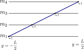
Figure 1: The contribution to the index of $P$ when the profile of $\Sigma(y)$ is a straight line. The straight profile crosses the mass level from negative to positive. Each crossing contributes to the index by $+1$. So the index is $+4$ in total.

When we choose the profile $\Sigma(y)$ freely, we always obtain the same index $\operatorname{ind}P=+4$. So the index is invariant under a continuous deformation of $\Sigma(y)$. (See Fig. 2.)

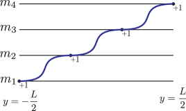
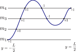
(a)		(b)

Figure 2: The index does not change by continuous deformations of the profile of $\Sigma(y)$ with the fixed boundary condition. (a) The kink profile which may be obtained after solving the BPS equations gives the same index as the straight line. (b) Even if a continuous deformation produces negative contributions to the index, additional positive contributions are also produced and the total contribution to the index remains the same as $+4$.

4.1.3 Evaluation of integral

Thus we have the indices for the $N_{f}=4$ case, and obtain the integration formula for the volume of the moduli space as

$${\rm Vol}\left({\mathcal{M}}^{1,4}_{1\to 4}\right)=\int_{-\infty}^{\infty}\frac{d\phi}{2\pi}\frac{1}{(i\phi)^{4}}e^{i\phi\beta\left(\frac{g^{2}c}{2}L-d\right)}.$$ (4.7)

This integral has a fourth order pole at $\phi=0$. We can perform this integral by using the following residue calculus with a suitable contour dictated by the convergence of $H,H^{\dagger}$ path integral

$$\int_{-\infty-i\epsilon}^{\infty-i\epsilon}\frac{d\phi}{2\pi i}\frac{1}{\phi^{n+1}}e^{i\phi B}=\begin{cases}\frac{1}{n!}(iB)^{n}&\text{if $B\geq 0$ and $n\geq 0$}\\ 0&\text{otherwise}\end{cases}.$$ (4.8)

Thus we obtain the volume of the moduli space

$${\rm Vol}\left({\mathcal{M}}^{1,4}_{1\to 4}\right)=\frac{1}{3!}\left(\frac{g^{2}c}{2}L-d\right)^{3},$$ (4.9)

when $\frac{g^{2}c}{2}L-d\geq 0$.

We next discuss implications of the result (4.9). If we consider the case $L\gg\frac{2d}{g^{2}c}$, where the size of the interval $L$ is sufficiently large in comparison with the width Kaplunovsky:1998vt ; Eto:2006ng ; Shifman:2002jm of the domain-wall $\frac{2d}{g^{2}c}$, then the volume is proportional to $\frac{L^{3}}{3!}$. This is nothing but a volume of the moduli space of three undistinguished points on the interval $L$. So we can regard the power of $(\frac{g^{2}c}{2}L-d)$ as the number of the BPS domain-walls on the interval (the dimension of the domain-wall moduli space). This agrees with the number of kinks which is depicted in Fig.2(a). Recalling that the order of pole comes from the index of $P$, so we can conclude that

$$\operatorname{ind}P=\text{(the number of BPS domain-walls)+1}.$$ (4.10)

We also understand this fact from another point of view. The index of $P$ is obtained from the equations $\mu_{c}=\mu_{c}^{\dagger}=0$ without imposing the other BPS equations $\mu_{r}=0$. Only after $\phi$ is integrated out, the equation $\mu_{r}=0$ is taken into account. The number of the domain-walls coincides with the dimension of the moduli space. Additional $+1$ of the index of $P$ is removed by the contour integral and the number reduces to the dimension of the moduli space. The dimension of the moduli space is also calculated by an index theorem where all of the BPS equations are considered. We have finally obtained the dimension of the moduli space after imposing the condition $\mu_{r}=0$. Thus we have done a correct evaluation of the moduli space volume by the contour integral of $\phi$.

Using similar arguments as above, we can easily extend our computation to the case where $N_{f}$ and the boundary conditions are general.

$${\rm Vol}\left({\mathcal{M}}^{1,N_{f}}_{i\to j}\right) = \int_{-\infty}^{\infty}\frac{d\phi}{2\pi}\frac{1}{(i\phi)^{j-i+1}}e^{i\phi\beta\left(\frac{g^{2}c}{2}L-d_{ij}\right)}$$ (4.11)

$$= \frac{\beta^{j-i}}{(j-i)!}\left(\frac{g^{2}c}{2}L-d_{ij}\right)^{j-i},$$

where $d_{ij}\equiv m_{j}-m_{i}$.

4.2 Non-Abelian domain-walls

The localization formula (3.31) says that the non-Abelian gauge group $U(N_{c})$ reduces to a product of the Abelian groups $U(1)^{N_{c}}$ at the fixed point set. So the localization formula for the non-Abelian gauge group is essentially a direct product of the formula for the Abelian group. In particular, the indices (number of walls) for each Abelian factor is determined by the boundary conditions as in Eq.(4.10). With this result for the indices ind$P$, Eq.(3.37) for the volume of the moduli space of the non-Abelian walls becomes

$${\rm Vol}\left({\mathcal{M}}^{N_{c},N_{f}}_{\vec{A}\to\vec{B}}\right)=\sum_{\sigma\in\mathfrak{S}_{N_{c}}}\prod_{a=1}^{N_{c}}\int_{-\infty}^{\infty}\frac{d\phi_{a}}{2\pi}\frac{(-1)^{|\sigma|}}{(i\phi_{a})^{B_{\sigma(a)}-A_{a}+1}}e^{i\phi_{a}\beta\left(\hat{L}-(m_{B_{\sigma(a)}}-m_{A_{a}})\right)}.$$ (4.12)

If some of the permutations of the boundary conditions satisfy $B_{\sigma(a)}-A_{a}<0$, the corresponding $\phi_{a}$ integral does not have a pole and vanishes. These boundary conditions $B_{\sigma(a)}-A_{a}<0$ correspond to non-BPS wall solutions. Although the non-BPS walls are in general contained in the $\phi_{a}$ integral (4.12), they give vanishing contributions. So the integral is finally restricted to a set of permutations $\mathfrak{S}^{\prime}_{N_{c}}$, which satisfy $\forall(B_{\sigma(a)}-A_{a})\geq 0$ (BPS wall conditions). The integral can be evaluated by

$${\rm Vol}\left({\mathcal{M}}^{N_{c},N_{f}}_{\vec{A}\to\vec{B}}\right)=\beta^{D}\sum_{\sigma\in\mathfrak{S}^{\prime}_{N_{c}}}\prod_{a=1}^{N_{c}}\frac{(-1)^{|\sigma|}}{(B_{\sigma(a)}-A_{a})!}\left(\hat{L}-(m_{B_{\sigma(a)}}-m_{A_{a}})\right)^{B_{\sigma(a)}-A_{a}},$$ (4.13)

where $D=\dim{\mathcal{M}}^{N_{c},N_{f}}_{\vec{A}\to\vec{B}}=\sum_{a=1}^{N_{c}}(B_{a}-A_{a})$ is the dimension of the moduli space.

It is interesting to note that the above volume formula of the non-Abelian domain-wall can be expressed by a determinant of a matrix ${\mathcal{T}}$

$${\rm Vol}\left({\mathcal{M}}^{N_{c},N_{f}}_{\vec{A}\to\vec{B}}\right)=\beta^{D}\det{\mathcal{T}}^{N_{c},N_{f}}_{\vec{A}\to\vec{B}},$$ (4.14)

where

$$\left({\mathcal{T}}^{N_{c},N_{f}}_{\vec{A}\to\vec{B}}\right)_{ab}=\left\{\begin{array}[]{ll}{\displaystyle\frac{1}{(B_{b}-A_{a})!}\left(\hat{L}-(m_{B_{b}}-m_{A_{a}})\right)^{B_{b}-A_{a}}}&\text{if }B_{b}\geq A_{a},\\ 0&\text{if }B_{b}<A_{a}.\end{array}\right.$$ (4.15)

We will call this matrix ${\mathcal{T}}$ as a transition matrix in the following.

Using the above formula, let us consider some concrete examples for the non-Abelian gauge group in order to understand the meaning of the volume formula (4.13). We first consider the case of $N_{c}=2$ and $N_{f}=4$ with the boundary condition $\Sigma(-L/2)=\operatorname{diag}(m_{1},m_{3})$ and $\Sigma(L/2)=\operatorname{diag}(m_{2},m_{4})$. The $\phi_{a}$ integral (4.13) for this boundary condition is given concretely by

$${\rm Vol}\left({\mathcal{M}}^{2,4}_{(1,3)\to(2,4)}\right) = \int\frac{d\phi_{1}}{2\pi}\frac{d\phi_{2}}{2\pi}\frac{e^{i\beta\phi_{1}(\hat{L}-(m_{2}-m_{1}))}}{(i\phi_{1})^{2}}\frac{e^{i\beta\phi_{2}(\hat{L}-(m_{4}-m_{3}))}}{(i\phi_{2})^{2}}$$ (4.16)

$$-\int\frac{d\phi_{1}}{2\pi}\frac{d\phi_{2}}{2\pi}\frac{e^{i\beta\phi_{1}(\hat{L}-(m_{4}-m_{1}))}}{(i\phi_{1})^{4}}\frac{e^{i\beta\phi_{2}(\hat{L}-(m_{2}-m_{3}))}}{(i\phi_{2})^{0}}.$$

The second term contains the anti-BPS wall configuration and the $\phi_{a}$ integral vanishes. So only the first term contributes to the volume. Thus we obtain

$${\rm Vol}\left({\mathcal{M}}^{2,4}_{(1,3)\to(2,4)}\right)=\beta^{2}(\hat{L}-(m_{2}-m_{1}))(\hat{L}-(m_{4}-m_{3})).$$ (4.17)

This result is essentially a direct product of independent Abelian walls. (See Fig. 3.) In this case, the $2\times 2$ transition matrix becomes

$${\mathcal{T}}^{2,4}_{(1,3)\to(2,4)}=\begin{pmatrix}\hat{L}-(m_{2}-m_{1})&\frac{1}{3!}(\hat{L}-(m_{4}-m_{1}))^{3}\\ 0&\hat{L}-(m_{2}-m_{1})\end{pmatrix}.$$ (4.18)

The determinant of this matrix (times $\beta^{2}$) precisely gives (4.17).

	-
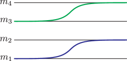
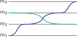
(a)		(b)

Figure 3: The possible domain-wall profiles of the boundary condition $\Sigma(-L/2)=\operatorname{diag}(m_{1},m_{3})$ and $\Sigma(L/2)=\operatorname{diag}(m_{2},m_{4})$ with the permutations. Solid line represents for the BPS profile while dashed line represents the anti-BPS one. The contribution from the non-BPS domain-wall profile which includes the anti-BPS domain-wall disappears from the sum of the volume evaluation.

Next example is almost the same as the previous case except for the boundary condition: $\Sigma(-L/2)=\operatorname{diag}(m_{1},m_{2})$ and $\Sigma(L/2)=\operatorname{diag}(m_{3},m_{4})$ in the case of $N_{c}=2$ and $N_{f}=4$. Similarly to the previous case, permutations of boundary conditions provide two contributions as shown in Fig. 4. Both of them now correspond to BPS configurations and are non-vanishing unlike the previous case

$${\rm Vol}\left({\mathcal{M}}^{2,4}_{(1,2)\to(3,4)}\right) = \int\frac{d\phi_{1}}{2\pi}\frac{d\phi_{2}}{2\pi}\frac{e^{i\beta\phi_{1}(\hat{L}-(m_{3}-m_{1}))}}{(i\phi_{1})^{3}}\frac{e^{i\beta\phi_{2}(\hat{L}-(m_{4}-m_{2}))}}{(i\phi_{2})^{3}}$$ (4.19)

$$-\int\frac{d\phi_{1}}{2\pi}\frac{d\phi_{2}}{2\pi}\frac{e^{i\beta\phi_{1}(\hat{L}-(m_{4}-m_{1}))}}{(i\phi_{1})^{4}}\frac{e^{i\beta\phi_{2}(\hat{L}-(m_{3}-m_{2}))}}{(i\phi_{2})^{2}}.$$

The second term corresponds to the case of two color lines intersecting each other, as shown in the Fig. 4(b). Evaluating the $\phi_{a}$ integral, we obtain

$${\rm Vol}\left({\mathcal{M}}^{2,4}_{(1,2)\to(3,4)}\right) = \beta^{4}\Bigg{\{}\frac{1}{4}(\hat{L}-(m_{3}-m_{1}))^{2}(\hat{L}-(m_{4}-m_{2}))^{2}$$ (4.20)

$$\qquad-\frac{1}{6}(\hat{L}-(m_{4}-m_{1}))^{3}(\hat{L}-(m_{3}-m_{2}))\Bigg{\}}.$$

This can be expressed by a determinant of the $2\times 2$ transition matrix as in Eq.(4.14)

$${\mathcal{T}}^{2,4}_{(1,2)\to(3,4)}=\begin{pmatrix}\frac{1}{2!}(\hat{L}-(m_{3}-m_{1}))^{2}&\frac{1}{3!}(\hat{L}-(m_{4}-m_{1}))^{3}\\ \hat{L}-(m_{3}-m_{2})&\frac{1}{2!}(\hat{L}-(m_{4}-m_{2}))^{2}\end{pmatrix}.$$ (4.21)

Let us examine the meaning of our result more closely. The kink-profiles such as in Fig. 4 may be understood to represent $\Sigma(y)$ connecting vacuum values given by boundary conditions. Taking for instance the wall connecting $m_{3}$ and $m_{4}$ in the upper line of Fig. 4(a), its position can only go to the right up to the other wall connecting $m_{2}$ and $m_{3}$ in the lower line, namely they are non-penetrable each other Isozumi:2004jc ; Eto:2006ng . This type of restriction gives an interesting behavior of moduli space volume, as illustrated in a concrete example in Appendix A. On the other hand, our volume formula is given in terms of $\phi_{a}$, the zero mode of $\Phi^{a}$, which is canonically conjugate to the variable $\Sigma^{a}$. The $\phi_{a}$ integral counts the number of domain walls in the $a$-th color line without particular restrictions on possible range of wall positions. Instead, our formula compensates the over-counting of integration range by subtracting appropriate contributions in the form of permutations of boundary conditions carrying a sign given by the intersection number of color lines, as shown in Fig. 4(b). Combining all contributions from permutations of boundary conditions, the volume is finally given in terms of the determinant of the transition matrix (4.14).

	-
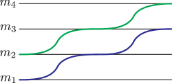
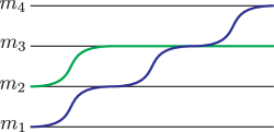
(a)		(b)

Figure 4: The possible domain-wall profiles of the boundary condition $\Sigma(-L/2)=\operatorname{diag}(m_{1},m_{2})$ and $\Sigma(L/2)=\operatorname{diag}(m_{3},m_{4})$ with the permutations. (a) The contribution with no color-line intersections. (b) The contribution with an intersection of two color lines, which carries a negative sign.

5 Duality between Non-Abelian Domain-walls

We have found a formula for evaluating the volume of the domain-wall moduli space. We here give a non-trivial check of our localization formula by examining duality relations between two different theories and boundary conditions. We take two different gauge theories: $G=U(N_{c})$ gauge group with $N_{f}$ flavors and $\tilde{G}=U(\tilde{N}_{c})$ gauge group with $N_{f}$ flavors, where $\tilde{N}_{c}\equiv N_{f}-N_{c}$. The boundary conditions of both theories should be chosen to connect complementary vacua as follows. If the boundary conditions of the original $G=U(N_{c})$ theory are $\vec{A}\to\vec{B}$, then the corresponding boundary conditions of the other $\tilde{G}=U(\tilde{N}_{c})$ theory should be $\overline{\vec{B}}\to\overline{\vec{A}}$, where $\overline{\vec{A}}$ and $\overline{\vec{B}}$ are the complement of $\vec{A}$ and $\vec{B}$, respectively. For example, the boundary condition $\vec{A}=(2,4,5)$ of $G=U(3)$ theory with $N_{f}=5$ flavors is complementary to the boundary condition $\overline{\vec{A}}=(1,3)$ of $\tilde{G}=U(2)$ with $N_{f}=5$ flavors. Let us call both theories with the complementary boundary conditions as dual theories.

In the strong coupling limit, the gauge theories become non-linear sigma models and two dual theories become identical Isozumi:2004va ; Antoniadis:1996ra . It has been demonstrated explicitly that the moduli spaces of domain-walls (in the infinite interval) have a one-to-one correspondence and become identical in the dual theories in the strong coupling limit Isozumi:2004va . Even in the finite gauge coupling, the moduli spaces of the domain-walls of these dual theories are topologically the same

$${\mathcal{M}}^{N_{c},N_{f}}_{\vec{A}\to\vec{B}}\simeq{\mathcal{M}}^{\tilde{N}_{c},N_{f}}_{\overline{\vec{B}}\to\overline{\vec{A}}},$$ (5.1)

but their metric and other properties are different Isozumi:2004va . Consequently the moduli space of domain-walls in these two theories are different at finite gauge coupling, but should become identical in the strong coupling limit. We need to specify the boundary condition for dual theories. The explicit formula of one-to-one correspondence of dual theories Isozumi:2004va suggests that the color-flavor locking of vacua should be chosen in such a way that those vacua occupied in dual theories should be the complement of each other. Namely among $N_{f}$ flavors, $N_{c}$ should be selected to specify a vacuum in $U(N_{c})$ gauge theory, whereas the remaining $\tilde{N}_{c}$ flavors should be selected in the dual $U(\tilde{N}_{c})$ gauge theory to give the dual boundary condition.

We will see that our results for the volume of moduli spaces for these two theories differ for finite gauge coupling, but become identical for strong coupling limit $g^{2}\to\infty$.

5.1 Abelian versus non-Abelian duality

First of all, let us consider duality between Abelian gauge group $G=U(1)$ and non-Abelian gauge group $\tilde{G}=U(N_{f}-1)$ with the $N_{f}$ flavors of the same ordered masses $m_{1},m_{2},\ldots,m_{N_{f}}$.

For the Abelian model, we take a boundary condition to be $\Sigma(-L/2)=m_{1}$ and $\Sigma(L/2)=m_{N_{f}}$ to obtain the maximal dimensions of the moduli space. Using the localization formula of the volume for this boundary condition, we obtain

$${\rm Vol}\left({\mathcal{M}}^{1,N_{f}}_{1\to N_{f}}\right)=\frac{\beta^{N_{f}-1}}{(N_{f}-1)!}\left(\hat{L}-d_{1,N_{f}}\right)^{N_{f}-1}.$$ (5.2)

The dual of the above Abelian model is the $\tilde{G}=U(N_{f}-1)$ gauge group with $N_{f}$ flavors. The dual boundary condition corresponds also to the maximal dimensions of the moduli space and is given by $\Sigma^{a}(-L/2)=m_{a}$ and $\Sigma^{a}(L/2)=m_{a+1}$ ($a=1,\ldots,N_{f}-1$). The transition matrix of this model becomes

$${\mathcal{T}}^{N_{f}-1,N_{f}}_{(1,2,\ldots,N_{f}-1)\to(2,3,\ldots,N_{f})}\\ =\begin{pmatrix}\hat{L}-d_{12}&\frac{1}{2!}(\hat{L}-d_{13})^{2}&\frac{1}{3!}(\hat{L}-d_{14})^{3}&\cdots&\frac{1}{(N_{f}-1)!}(\hat{L}-d_{1,N_{f}})^{N_{f}-1}\\ 1&\hat{L}-d_{23}&\frac{1}{2!}(\hat{L}-d_{24})^{2}&\cdots&\frac{1}{(N_{f}-2)!}(\hat{L}-d_{2,N_{f}})^{N_{f}-2}\\ 0&1&\hat{L}-d_{34}&\cdots&\frac{1}{(N_{f}-3)!}(\hat{L}-d_{3,N_{f}})^{N_{f}-3}\\ \vdots&\vdots&\vdots&\ddots&\vdots\\ 0&0&0&\cdots&\hat{L}-d_{N_{f},N_{f}-1}\end{pmatrix}.$$ (5.3)

The volume of the moduli space can be evaluated from the determinant of the above transition matrix as

$${\rm Vol}\left({\mathcal{M}}^{N_{f}-1,N_{f}}_{(1,2,\ldots,N_{f}-1)\to(2,3,\ldots,N_{f})}\right)=\beta^{N_{f}-1}\operatorname{Det}{\mathcal{T}}^{N_{f}-1,N_{f}}_{(1,2,\ldots,N_{f}-1)\to(2,3,\ldots,N_{f})}.$$ (5.4)

The boundary conditions and typical kink profiles of Abelian and non-Abelian theories with $N_{f}$ flavors are depicted in Fig. 5.

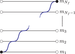
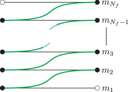
(a)		(b)

Figure 5: The duality between Abelian and non-Abelian theories. (a) Abelian theory with $N_{f}$ flavors and the boundary condition of $\Sigma(-L/2)=m_{1}$ and $\Sigma(L/2)=m_{N_{f}}$. (b) $G=U(N_{f}-1)$ non-Abelian theory with $N_{f}$ flavors and the boundary condition of $\Sigma(-L/2)=\operatorname{diag}(m_{1},m_{2},m_{3},\ldots,m_{N_{f}-1})$ and $\Sigma(L/2)=\operatorname{diag}(m_{2},m_{3},\ldots,m_{N_{f}-1},m_{N_{f}})$. Black and white circles represent vacua specified by the boundary conditions and their complements, respectively.

The volume (5.2) and (5.4) are different from each other in a general coupling region. In Appendix A, we will explicitly demonstrate this difference in the simplest case of $N_{f}=3$ with $N_{c}=1$ and $N_{c}=2$ as a concrete example. We will also show there that the results agree with those of a direct calculation using the rigid-rod approximation Eto:2007aw .

On the other hand, in the strong coupling limit $g^{2}\to\infty$ where $\hat{L}=\frac{g^{2}c}{2}L$ becomes large, we find

$${\rm Vol}\left({\mathcal{M}}^{1,N_{f}}_{1\to N_{f}}\right)\approx\frac{\beta^{N_{f}-1}}{(N_{f}-1)!}\hat{L}^{N_{f}-1},$$ (5.5)

and

$${\rm Vol}\left({\mathcal{M}}^{N_{f}-1,N_{f}}_{(1,2,\ldots,N_{f}-1)\to(2,3,\ldots,N_{f})}\right)\approx\frac{\beta^{N_{f}-1}}{(N_{f}-1)!}\hat{L}^{N_{f}-1}.$$ (5.6)

(See Appendix B.) Thus the volumes agree with each other in the strong coupling limit as expected by the duality. This result means that the leading terms of the volume in $\hat{L}$ coincide in two different models, including a combinatorial coefficient. This fact is highly non-trivial and suggests our localization formula of the volume expressed by the determinant works correctly.

In this case, the moduli spaces of both theories are topologically isomorphic to a complex projective space $\mathbb{C}P^{N_{f}-1}$

$${\mathcal{M}}^{1,N_{f}}_{1\to N_{f}}\simeq{\mathcal{M}}^{N_{f}-1,N_{f}}_{(1,2,\ldots,N_{f}-1)\to(2,3,\ldots,N_{f})}\simeq\mathbb{C}P^{N_{f}-1}.$$ (5.7)

Indeed, the volumes (5.5) and (5.6) represent a rigid volume of $\mathbb{C}P^{N_{f}-1}$ with a “size” $\frac{\beta\hat{L}}{2\pi}$.

5.2 Non-Abelian versus non-Abelian duality

To give another non-trivial check, let us consider a duality between two non-Abelian gauge groups. One model is $G=U(3)$ with $N_{f}=5$ and the other dual model is $\tilde{G}=U(2)$ with $N_{f}=5$. Firstly, we consider the complementary boundary conditions: $\Sigma(-L/2)=\operatorname{diag}(m_{1},m_{2},m_{3})$ and $\Sigma(L/2)=\operatorname{diag}(m_{3},m_{4},m_{5})$ for $G=U(3)$ theory, and $\Sigma(-L/2)=\operatorname{diag}(m_{1},m_{2})$ and $\Sigma(L/2)=\operatorname{diag}(m_{4},m_{5})$ for $\tilde{G}=U(2)$ theory. These boundary conditions maximize the dimension of the moduli space for the present dual theories.

The transition matrices of both theories are

$${\mathcal{T}}^{3,5}_{(1,2,3)\to(3,4,5)}=\begin{pmatrix}\frac{1}{2!}(\hat{L}-d_{13})^{2}&\frac{1}{3!}(\hat{L}-d_{14})^{3}&\frac{1}{4!}(\hat{L}-d_{15})^{4}\\ \hat{L}-d_{23}&\frac{1}{2!}(\hat{L}-d_{24})^{2}&\frac{1}{3!}(\hat{L}-d_{25})^{3}\\ 1&\hat{L}-d_{34}&\frac{1}{2!}(\hat{L}-d_{35})^{2}\end{pmatrix},$$ (5.8)

and

$${\mathcal{T}}^{2,5}_{(1,2)\to(4,5)}=\begin{pmatrix}\frac{1}{3!}(\hat{L}-d_{14})^{3}&\frac{1}{4!}(\hat{L}-d_{15})^{4}\\ \frac{1}{2!}(\hat{L}-d_{24})^{2}&\frac{1}{3!}(\hat{L}-d_{25})^{3}\end{pmatrix}.$$ (5.9)

The boundary conditions and typical kink profiles of both non-Abelian theories are shown in Fig. 6.

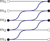
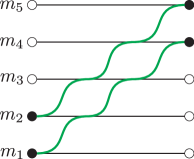
(a)		(b)

Figure 6: The duality between non-Abelian theories. (a) $G=U(3)$ non-Abelian theory with $N_{f}=5$ and the boundary condition of $\Sigma(-L/2)=\operatorname{diag}(m_{1},m_{2},m_{3})$ and $\Sigma(L/2)=\operatorname{diag}(m_{3},m_{4},m_{5})$. (b) $G=U(2)$ non-Abelian theory with $N_{f}=5$ and the boundary condition of $\Sigma(-L/2)=\operatorname{diag}(m_{1},m_{2})$ and $\Sigma(L/2)=\operatorname{diag}(m_{4},m_{5})$. The boundary conditions are given to connect complementary vacua (exchanging the role of black and white circles).

The volumes of both theories coincide with each other in the strong coupling limit

$${\rm Vol}\left({\mathcal{M}}^{3,5}_{(1,2,3)\to(3,4,5)}\right)=\beta^{6}\operatorname{Det}{\mathcal{T}}^{3,5}_{(1,2,3)\to(3,4,5)}=\frac{\beta^{6}}{144}\hat{L}^{6}+{\mathcal{O}}(\hat{L}^{5}),$$ (5.10)

and

$${\rm Vol}\left({\mathcal{M}}^{2,5}_{(1,2)\to(4,5)}\right)=\beta^{6}\operatorname{Det}{\mathcal{T}}^{2,5}_{(1,2)\to(4,5)}=\frac{\beta^{6}}{144}\hat{L}^{6}+{\mathcal{O}}(\hat{L}^{5}).$$ (5.11)

This result shows that the (complex) dimension of the moduli space is 6.

In this maximal dimension case, the moduli spaces are isomorphic to a complex Grassmann manifold (Grassmannian)

$${\mathcal{M}}^{3,5}_{(1,2,3)\to(3,4,5)}\simeq G_{3,5}\simeq G_{2,5}\simeq{\mathcal{M}}^{2,5}_{(1,2)\to(4,5)},$$ (5.12)

where $G_{N_{c},N_{f}}$ is expressed by a coset space

$$G_{N_{c},N_{f}}\equiv\frac{U(N_{f})}{U(N_{c})\times U(\tilde{N}_{c})}.$$ (5.13)

The volume of the Grassmannian of unit “size” is obtained from a quotient of unitary group volumes Macdonald ; Fujii ; Ooguri:2002gx (see also Appendix in Miyake:2011yr )

$${\rm Vol}(G_{N_{c},N_{f}})=\frac{\prod_{j=1}^{N_{c}}(j-1)!\times\prod_{k=1}^{\tilde{N}_{c}}(k-1)!}{\prod_{i=1}^{N_{f}}(i-1)!}(2\pi)^{N_{c}\tilde{N}_{c}}.$$ (5.14)

The volume of the Grassmannian is invariant under exchanging $N_{c}$ and $\tilde{N}_{c}$.

Using this formula, we notice that the leading term of the volumes (5.10) and (5.11) are nothing but the volume of the Grassmannian $G_{3,5}$ or $G_{2,5}$ with “size” $\frac{\beta\hat{L}}{2\pi}$, since

$${\rm Vol}(G_{3,5})={\rm Vol}(G_{2,5})=\frac{2!1!\times 1!}{4!3!2!1!}(2\pi)^{6}=\frac{1}{144}(2\pi)^{6}.$$ (5.15)

Therefore our results are consistent with the notion that the moduli spaces of the domain-walls in dual theories asymptotically coincide with the Grassmannian $G_{3,5}$ or $G_{2,5}$ with the standard metric, but the differential structure (metric) is deformed by the sub-leading terms in $\hat{L}$. These non-trivial agreements strongly suggest that the duality between different non-Abelian gauge theories is valid in the strong coupling region.

As another example, let us next consider a different boundary condition with non-maximal dimensions of moduli space : $\Sigma(-L/2)=\operatorname{diag}(m_{1},m_{2},m_{3})$ and $\Sigma(L/2)=\operatorname{diag}(m_{2},m_{4},m_{5})$ for $G=U(3)$ theory as the boundary condition in one theory, and $\Sigma(-L/2)=\operatorname{diag}(m_{1},m_{3})$ and $\Sigma(L/2)=\operatorname{diag}(m_{4},m_{5})$ for $\tilde{G}=U(2)$ theory as the corresponding dual. The boundary conditions and typical kink profiles of both non-Abelian theories are shown in Fig. 7.

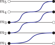
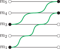
(a)		(b)

Figure 7: The duality between non-Abelian theories with a non-maximal boundary condition. (a) $G=U(3)$ non-Abelian theory with $N_{f}=5$ and the boundary condition of $\Sigma(-L/2)=\operatorname{diag}(m_{1},m_{2},m_{3})$ and $\Sigma(L/2)=\operatorname{diag}(m_{2},m_{4},m_{5})$. (b) $G=U(2)$ non-Abelian theory with $N_{f}=5$ and the boundary condition of $\Sigma(-L/2)=\operatorname{diag}(m_{1},m_{3})$ and $\Sigma(L/2)=\operatorname{diag}(m_{4},m_{5})$.

The transition matrices of both theories with these boundary conditions are

$${\mathcal{T}}^{3,5}_{(1,2,3)\to(2,4,5)}=\begin{pmatrix}\hat{L}-d_{12}&\frac{1}{3!}(\hat{L}-d_{14})^{3}&\frac{1}{4!}(\hat{L}-d_{15})^{4}\\ 1&\frac{1}{2!}(\hat{L}-d_{24})^{2}&\frac{1}{3!}(\hat{L}-d_{25})^{3}\\ 0&\hat{L}-d_{34}&\frac{1}{2!}(\hat{L}-d_{35})^{2}\end{pmatrix},$$ (5.16)

and

$${\mathcal{T}}^{2,5}_{(1,3)\to(4,5)}=\begin{pmatrix}\frac{1}{3!}(\hat{L}-d_{14})^{3}&\frac{1}{4!}(\hat{L}-d_{15})^{4}\\ \hat{L}-d_{34}&\frac{1}{2!}(\hat{L}-d_{35})^{2}\end{pmatrix}.$$ (5.17)

The volumes of both theories coincide with each other in the strong coupling limit

$${\rm Vol}\left({\mathcal{M}}^{3,5}_{(1,2,3)\to(2,4,5)}\right)=\beta^{5}\operatorname{Det}{\mathcal{T}}^{3,5}_{(1,2,3)\to(2,4,5)}=\frac{\beta^{5}}{24}\hat{L}^{5}+{\mathcal{O}}(\hat{L}^{4}),$$ (5.18)

and

$${\rm Vol}\left({\mathcal{M}}^{2,5}_{(1,3)\to(4,5)}\right)=\beta^{5}\operatorname{Det}{\mathcal{T}}^{2,5}_{(1,3)\to(4,5)}=\frac{\beta^{5}}{24}\hat{L}^{5}+{\mathcal{O}}(\hat{L}^{4}).$$ (5.19)

This result shows that the (complex) dimension of the moduli space is 5, which is smaller than the maximal dimension 6, as expected. So the moduli space for the present boundary conditions should be a complex sub-manifold of the Grassmannian $G_{3,5}\simeq G_{2,5}$.

In Appendix B, we evaluate the asymptotic behavior of the volume of the moduli space in the case of maximal dimensions for the general $N_{c}$ gauge theories with $N_{f}$ flavors to obtain

$$\begin{split}{\rm Vol}\left({\mathcal{M}}^{N_{c},N_{f}}_{(1,2,\ldots,N_{c})\to(\tilde{N}_{c}+1,\ldots,N_{f}-1,N_{f})}\right)&=\frac{\prod_{j=1}^{N_{c}}(j-1)!\times\prod_{k=1}^{\tilde{N}_{c}}(k-1)!}{\prod_{i=1}^{N_{f}}(i-1)!}\left(\beta\hat{L}\right)^{N_{c}\tilde{N}_{c}}+\cdots,\\ {\rm Vol}\left({\mathcal{M}}^{\tilde{N}_{c},N_{f}}_{(1,2,\ldots,\tilde{N}_{c})\to(N_{c}+1,\ldots,N_{f}-1,N_{f})}\right)&=\frac{\prod_{j=1}^{N_{c}}(j-1)!\times\prod_{k=1}^{\tilde{N}_{c}}(k-1)!}{\prod_{i=1}^{N_{f}}(i-1)!}\left(\beta\hat{L}\right)^{N_{c}\tilde{N}_{c}}+\cdots.\end{split}$$ (5.20)

This result shows that there exists a duality relation between two different domain-wall theories in the strong coupling region.

6 T-duality to Vortex on Cylinder

In this section, we discuss another kind of duality between the domain-walls and vortices. As discussed in Eto:2006mz ; Eto:2007aw , there exists a T-duality relation between vortices on a cylinder and domain-walls on the interval. We here would like to show that the volume of the moduli space exhibits this T-duality. As a base space we consider a cylinder, which is a two-dimensional surface of a circle $S^{1}$ with the radius $\beta$ times an interval $I$ with the length $L$.

To see this duality, we start with the simplest case: vortices in $U(1)$ gauge theory with a single charged matter, which are called Abelian local vortices, or Abrikosov-Nielsen-Olesen (ANO) vortices Abrikosov:1956sx . If there are $k$ vortices on the cylinder, the vortices are mapped to $k$ domain-walls (kinks) on the interval with the length $L$ by the T-duality. The charged matters are mapped to the matter branes Eto:2004vy and we can regard mass differences for each kink to be $1/\beta$, which is the radius of the dual circle in the domain-wall picture. (See Fig. 8.)

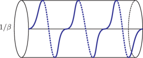
	$\Rightarrow$
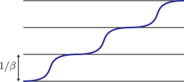
(a)		(b)

Figure 8: T-dual picture of the vortex on a cylinder. The $k$ vortices on the cylinder are dual to the domain-walls wrapping $k$-times around the circle. (a) A covering space of the $k$ domain-walls on the cylinder. (b) The $k$ domain-walls in the infinite number of flavors of the mass difference $1/\beta$. They are equivalent.

The total mass difference between the boundary conditions at $y=-L/2$ and at $y=L/2$ is $k/\beta$. So we can derive the integral formula for the volume of this domain-wall moduli space as

$${\rm Vol}\left({\mathcal{M}}^{1,1}_{k}\right) = \int_{-\infty}^{\infty}\frac{d\phi}{2\pi}\frac{1}{(i\phi)^{k+1}}e^{i\phi\beta\left(\hat{L}-\frac{k}{\beta}\right)}$$ (6.1)

$$= \frac{1}{k!}\left(\beta\hat{L}-k\right)^{k}.$$

Recalling that the area of the cylinder in the vortex picture is given by ${\mathcal{A}}=2\pi\beta L$ and that $\hat{L}=g^{2}cL/2$ in Eq.(3.36), the volume (6.1) is equivalent to the volume of the ANO vortices on the cylinder

$${\rm Vol}\left({\mathcal{M}}^{1,1}_{k}\right)=\frac{1}{k!}\left(\frac{g^{2}c}{4\pi}{\mathcal{A}}-k\right)^{k},$$ (6.2)

where we can regard $g$ and $c$ as the gauge coupling and the FI parameter in the two-dimensional vortex system, respectively, since the combination $g^{2}c$ is invariant under the T-duality. In the large area limit ${\mathcal{A}}\to\infty$, the volume is proportional to ${\mathcal{A}}^{k}/k!$, which is the volume of the symmetric product space of the cylinder $(S^{1}\times I)^{k}/\mathfrak{S}_{k}$. This is consistent with the point-like behavior of the vortex in the large area limit.

Now let us consider the Abelian $k$ vortices with $N_{f}$ matter fields of identical charges. This is called Abelian semi-local vortices. In the vortex side, the masses of the charged matters are degenerate and they are T-dual to degenerate vacua in the domain-wall picture. Since it is subtle to treat the degenerate masses in the domain-wall side Eto:2008dm , we split the masses of the $N_{f}$ matters by giving small mass differences $\varepsilon$.

There are two different types of domain-walls in this $N_{f}$ flavor case. One type comes from the $k$ vortices, which becomes “large” domain-walls with the mass difference $1/\beta$. The other type is “small” domain-walls connecting the small mass differences $\varepsilon$. The number of the large domain-walls is always $k$, since they are $k$ winding domain-walls around the cylinder. The number of small domain-walls varies from $(k-1)\times(N_{f}-1)$ to $(k+1)\times(N_{f}-1)$, depending on the boundary conditions at $y=-L/2$ and $y=L/2$. So the total number of domain-walls with $N_{f}$ charged matters varies from $kN_{f}-(N_{f}-1)$ to $kN_{f}+(N_{f}-1)$, where we have assumed $k>0$. We denote this number by $kN_{f}+n$, where $n=-(N_{f}-1),\ldots,+(N_{f}-1)$ if $k>0$ . This means that the index for the domain-walls is $kN_{f}+n+1$. Note here that $n$ is determined by the number of the small domain-walls adjacent to the boundaries (boundary condition of the domain-walls). An example of the domain-wall configuration is shown in Fig. 9.

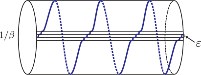
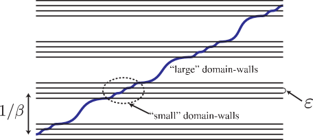
Figure 9: T-dual picture of the vortex on the cylinder with $N_{f}>1$ (Abelian semi-local vortex). The $k$ vortices on the cylinder are dual to the large domain-walls wrapping $k$-times around the circle, and the multiple $N_{f}$ flavors produce the small domain-walls with the small mass differences $\varepsilon$. We depict the case of $N_{f}=4$ and $k=3$. The number of the small domain-walls is 10 and the total number of the domain-walls is $10+3=3\times 4+1$, that is, $n=1$ in this example.

Noting that the mass difference of each one of the large and small domain-wall is $1/\beta-(N_{f}-1)\varepsilon$ and $\varepsilon$, respectively, we find the total mass difference of $k$ large domain-walls and $k(N_{f}-1)+n$ small domain-walls is $k\times(1/\beta-(N_{f}-1)\varepsilon)+(k(N_{f}-1)+n)\times\varepsilon=k/\beta+n\varepsilon$. Then, applying the localization formula to the above domain-wall configuration, we obtain the volume formula

$${\rm Vol}\left({\mathcal{M}}^{1,N_{f}}_{k}(S^{1}\times I)\right) = \int_{-\infty}^{\infty}\frac{d\phi}{2\pi}\frac{1}{(i\phi)^{kN_{f}+n+1}}e^{i\phi\beta\left(\hat{L}-\frac{k}{\beta}-n\varepsilon\right)}$$ (6.3)

$$= \frac{1}{(kN_{f}+n)!}\left(\beta\hat{L}-k-n\beta\varepsilon\right)^{kN_{f}+n}$$

$$= \frac{1}{(kN_{f}+n)!}\left({\hat{\mathcal{A}}}-k-n\beta\varepsilon\right)^{kN_{f}+n},$$

where we have defined ${\hat{\mathcal{A}}}\equiv\beta\hat{L}=\frac{g^{2}c}{4\pi}{\mathcal{A}}$. In the $\varepsilon\to 0$ limit, we find

$${\rm Vol}\left({\mathcal{M}}^{1,N_{f}}_{k}(S^{1}\times I)\right)=\frac{1}{(kN_{f}+n)!}\left({\hat{\mathcal{A}}}-k\right)^{kN_{f}+n}.$$ (6.4)

We can see that the above volume is the same as the volume of the moduli space of Abelian semi-local vortices with $N_{f}$ flavors on the sphere Miyake:2011yr if $n=N_{f}-1$.

In the large area limit ${\mathcal{A}}\to\infty$, the volume of the moduli space of the vortices on the cylinder (dual to the large and small domain-walls) is proportional to ${\mathcal{A}}^{kN_{f}+n}$. We do not know an explicit formula for the volume of the moduli space of the vortices on the cylinder, but this large area behavior suggests that the dimension of the moduli space of the vortex is $N_{f}+n$ and the index of the operator ${\mathcal{D}}_{\bar{z}}$ on the cylinder with the appropriate boundary condition, which counts the number of zero modes of the Higgs fields obeying ${\mathcal{D}}_{\bar{z}}H=0$ and determines the power of ${\mathcal{A}}$ via the contour integral, is $N_{f}+n+1$. So we expect that the index of the operator ${\mathcal{D}}_{\bar{z}}$ on the cylinder may be given by the Atiyah-Patodi-Singer index theorem AtiyahPatodiSinger

$$\begin{split}\operatorname{ind}{\mathcal{D}}_{\bar{z}}&=N_{f}\int_{S^{1}\times I}F-\frac{N_{f}}{2}\left[\eta(S^{1}_{R})-\eta(S^{1}_{L})\right]\\ &=kN_{f}+\left\lfloor N_{f}\left(\oint_{S^{1}_{R}}A-\oint_{S^{1}_{L}}A\right)\right\rfloor+1\\ &=kN_{f}+n+1,\end{split}$$ (6.5)

where $S^{1}_{R}$ and $S^{1}_{L}$ are the right and left boundaries of the cylinder, respectively, $\eta$ is the eta-invariant at the boundaries, and $\lfloor x\rfloor$ stands for the floor function which gives the largest integer not greater than $x$. The index theorem implies that the value of $n$ in Eq.(6.5) for vortices on the cylinder is also limited to be $-(N_{f}-1)\leq n\leq+(N_{f}-1)$ because of the T-duality. We expect that $n$ is determined by the holonomies at the boundaries of the cylinder. To see a precise correspondence between $n$ and holonomies, we need further investigation of the moduli of the vortex on the cylinder.

Finally, we discuss an extension of the above observations in the Abelian case to the non-Abelian case. As explained in the previous sections, the evaluation of the volume of the non-Abelian domain-wall moduli space can be reduced to a sum of products of the Abelian ones. So the T-dualized domain-walls of the non-Abelian vortex can also be decomposed into the Abelian ones. In this decomposition, we have to take into account the permutations of the boundary conditions for each Abelian component. The boundary condition is labeled by the integer $n$, which reflects the different number of the small domain-walls, as explained above. Thus each Abelian part of the domain-walls is labeled by the decomposed vortex charge $k_{a}$ and the integer $n_{a}$ associated with the boundary conditions, where $a$ runs over the rank of $U(N_{c})$, namely $a=1,\ldots,N_{c}$ and $k_{a}$ satisfies $k=\sum_{a=1}^{N_{c}}k_{a}$.

Thus, using the decomposition, we obtain the localization formula for the volume of the moduli space of the T-dualized non-Abelian vortex on the cylinder

$${\rm Vol}\left({\mathcal{M}}^{N_{c},N_{f}}_{k}(S^{1}\times I)\right) = \sum_{\vec{k},\vec{n}}(-1)^{|\sigma(\vec{k},\vec{n})|}\prod_{a=1}^{N_{c}}\int_{-\infty}^{\infty}\frac{d\phi_{a}}{2\pi}\frac{1}{(i\phi_{a})^{k_{a}N_{f}+n_{a}+1}}e^{i\phi_{a}\beta\left(\hat{L}-\frac{k_{a}}{\beta}-n_{a}\varepsilon\right)}$$

$$= \sum_{\vec{k},\vec{n}}(-1)^{|\sigma(\vec{k},\vec{n})|}\prod_{a=1}^{N_{c}}\frac{1}{(k_{a}N_{f}+n_{a})!}\left(\beta\hat{L}-k_{a}-n_{a}\beta\varepsilon\right)^{k_{a}N_{f}+n_{a}}$$

$$= \sum_{\vec{k},\vec{n}}(-1)^{|\sigma(\vec{k},\vec{n})|}\prod_{a=1}^{N_{c}}\frac{1}{(k_{a}N_{f}+n_{a})!}\left({\hat{\mathcal{A}}}-k_{a}-n_{a}\beta\varepsilon\right)^{k_{a}N_{f}+n_{a}},$$

where $\vec{k}$ are all possible $N_{c}$ component integer vectors satisfying $k=\sum_{a=1}^{N_{c}}k_{a}$ and with an ordering of $k_{1}\geq k_{2}\geq\cdots\geq k_{N_{c}}$, and $\vec{n}$ are varied in the given boundary conditions. The signature of each term depends on the order of the permutations $\sigma(\vec{k},\vec{n})$ of the boundary conditions determined by $\vec{k}$ and $\vec{n}$. The signature $(-1)^{|\sigma(\vec{k},\vec{n})|}$ is given by the parity of the intersection number of the $N_{c}$ color lines. The volume of the moduli space of the non-Abelian vortex on the cylinder may be obtained in the limit of $\varepsilon\to 0$. This formula also should be directly checked from the localization theorem for the vortex on the cylinder with the boundary conditions of the various holonomies.

To see the above construction concretely, let us consider only an example of $N_{c}=2$ and general $N_{f}$ for simplicity in the following, since the number of charge partitions increases rapidly for large $N_{c}$. We also take a trivial boundary condition, namely, $(1,2)\to(1,2)$.

First, for $k=0$, there is no partition of the charges, namely $(k_{1},k_{2})=(0,0)$. And also there is no choice of the boundary conditions. In the T-dual picture of domain-walls, this means that there exists no domain-wall, but the volume of the moduli space gives a finite contribution

$${\rm Vol}\left({\mathcal{M}}^{2,N_{f}}_{0}(S^{1}\times I)\right)=1.$$ (6.7)

This should provide the relative normalization of the volume.

For $k=1$, there are two partitions of the charges, which are $\vec{k}=(1,0)$. For this partition, there are two permutations of the boundary conditions, that give $\vec{n}=\{(-1,+1),(0,0)\}$. Thus the summation over all possible combinations of the charges and the boundary conditions gives the volume of the moduli space of the non-Abelian domain-walls

$$\begin{split}{\rm Vol}\left({\mathcal{M}}^{2,N_{f}}_{1}(S^{1}\times I)\right)&=-\frac{2}{N_{f}!}\left(\hat{\mathcal{A}}-1\right)^{N_{f}}+\frac{1}{(N_{f}-1)!}\left(\hat{\mathcal{A}}-1+\hat{\varepsilon}\right)^{N_{f}-1}\left(\hat{\mathcal{A}}-\hat{\varepsilon}\right)\end{split}$$ (6.8)

if $\hat{\mathcal{A}}>1$, where we define $\hat{\varepsilon}\equiv\beta\varepsilon$. The volume of the moduli space of the vortices is obtained in the limit of $\hat{\varepsilon}\to 0$.

For $k=2$, we have the choices of the charges and boundary conditions as $\vec{k}=\{(2,0),(1,1)\}$ and $\vec{n}=\{(0,0),(-1,1)\}$. Then the volume becomes

$$\begin{split}{\rm Vol}\left({\mathcal{M}}^{2,N_{f}}_{2}(S^{1}\times I)\right)&=\frac{2}{(2N_{f})!}\left(\hat{\mathcal{A}}-2\right)^{2N_{f}}\\ &\quad-\frac{1}{(2N_{f}-1)!}\left(\hat{\mathcal{A}}-2+\hat{\varepsilon}\right)^{2N_{f}-1}\left(\hat{\mathcal{A}}-\hat{\varepsilon}\right)\\ &\quad+\frac{1}{N_{f}!N_{f}!}\left(\hat{\mathcal{A}}-1\right)^{2N_{f}}\\ &\quad-\frac{1}{(N_{f}+1)!(N_{f}-1)!}\left(\hat{\mathcal{A}}-1-\hat{\varepsilon}\right)^{N_{f}+1}\left(\hat{\mathcal{A}}-1+\hat{\varepsilon}\right)^{N_{f}-1},\end{split}$$ (6.9)

if $\hat{\mathcal{A}}>2$.

Similarly, we obtain

$$\begin{split}{\rm Vol}\left({\mathcal{M}}^{2,N_{f}}_{3}(S^{1}\times I)\right)&=-\frac{2}{(3N_{f})!}\left({\hat{\mathcal{A}}}-3\right)^{3N_{f}}\\ &\quad+\frac{1}{(3N_{f}-1)!}\left({\hat{\mathcal{A}}}-3+\hat{\varepsilon}\right)^{3N_{f}-1}\left({\hat{\mathcal{A}}}-\hat{\varepsilon}\right)\\ &\quad-\frac{2}{(2N_{f})!N_{f}!}\left({\hat{\mathcal{A}}}-2\right)^{2N_{f}}\left({\hat{\mathcal{A}}}-1\right)^{N_{f}}\\ &\quad+\frac{1}{(2N_{f}+1)!(N_{f}-1)!}\left({\hat{\mathcal{A}}}-2-\hat{\varepsilon}\right)^{2N_{f}+1}\left({\hat{\mathcal{A}}}-1+\hat{\varepsilon}\right)^{N_{f}-1}\\ &\quad+\frac{1}{(2N_{f}-1)!(N_{f}+1)!}\left({\hat{\mathcal{A}}}-2+\hat{\varepsilon}\right)^{2N_{f}-1}\left({\hat{\mathcal{A}}}-1-\hat{\varepsilon}\right)^{N_{f}+1}\end{split}$$ (6.10)

if $\hat{\mathcal{A}}>3$ for $k=3$, and

$$\begin{split}{\rm Vol}\left({\mathcal{M}}^{2,N_{f}}_{4}(S^{1}\times I)\right)&=\frac{2}{(4N_{f})!}\left({\hat{\mathcal{A}}}-4\right)^{4N_{f}}\\ &\quad-\frac{1}{(4N_{f}-1)!}\left({\hat{\mathcal{A}}}-4+\hat{\varepsilon}\right)^{4N_{f}-1}\left({\hat{\mathcal{A}}}-\hat{\varepsilon}\right)\\ &\quad+\frac{2}{(3N_{f})!N_{f}!}\left({\hat{\mathcal{A}}}-3\right)^{3N_{f}}\left({\hat{\mathcal{A}}}-1\right)^{N_{f}}\\ &\quad-\frac{1}{(3N_{f}+1)!(N_{f}-1)!}\left({\hat{\mathcal{A}}}-3-\hat{\varepsilon}\right)^{3N_{f}+1}\left({\hat{\mathcal{A}}}-1+\hat{\varepsilon}\right)^{N_{f}-1}\\ &\quad-\frac{1}{(3N_{f}-1)!(N_{f}+1)!}\left({\hat{\mathcal{A}}}-3+\hat{\varepsilon}\right)^{3N_{f}-1}\left({\hat{\mathcal{A}}}-1-\hat{\varepsilon}\right)^{N_{f}+1}\\ &\quad+\frac{1}{(2N_{f})!(2N_{f})!}\left({\hat{\mathcal{A}}}-2\right)^{4N_{f}}\\ &\quad-\frac{1}{(2N_{f}+1)!(2N_{f}-1)!}\left({\hat{\mathcal{A}}}-2-\hat{\varepsilon}\right)^{2N_{f}+1}\left({\hat{\mathcal{A}}}-2+\hat{\varepsilon}\right)^{2N_{f}-1},\end{split}$$ (6.11)

if $\hat{\mathcal{A}}>4$ for $k=4$.

So far, we have considered the general number of flavors $N_{f}$ with the $U(2)$ gauge group. The volume of the moduli space of $k$ vortices is a complicated $kN_{f}$-th order polynomial in ${\hat{\mathcal{A}}}$. However, setting $N_{f}=N_{c}=2$, we see the order of polynomial of the volume remarkably reduces. The vortices in this situation ($N_{f}=N_{c}$) is called non-Abelian local vortices.

Putting $N_{f}=N_{c}=2$ into the results (6.7)-(6.11) for general $N_{f}$, we find the volume of the moduli space of non-Abelian local vortices on the cylinder as

$${\rm Vol}\left({\mathcal{M}}^{2,2}_{0}(S^{1}\times I)\right) = 1,$$

$${\rm Vol}\left({\mathcal{M}}^{2,2}_{1}(S^{1}\times I)\right) = \hat{\mathcal{A}}-1+\hat{\varepsilon}-\hat{\varepsilon}^{2},$$

$${\rm Vol}\left({\mathcal{M}}^{2,2}_{2}(S^{1}\times I)\right) = \frac{1}{2}\hat{\mathcal{A}}^{2}-\left(\frac{5}{3}-\hat{\varepsilon}+\hat{\varepsilon}^{2}\right)\hat{\mathcal{A}}+\frac{17}{12}-\frac{5}{3}\hat{\varepsilon}+2\hat{\varepsilon}^{2}-\frac{2}{3}\hat{\varepsilon}^{3}+\frac{1}{3}\hat{\varepsilon}^{4},$$

$${\rm Vol}\left({\mathcal{M}}^{2,2}_{3}(S^{1}\times I)\right) = \frac{1}{6}{\hat{\mathcal{A}}}^{3}-\frac{1}{2}\left(\frac{7}{3}-\hat{\varepsilon}+\hat{\varepsilon}^{2}\right){\hat{\mathcal{A}}}^{2}$$

$$+\left(\frac{331}{120}-\frac{7}{3}\hat{\varepsilon}+\frac{8}{3}\hat{\varepsilon}^{2}-\frac{2}{3}\hat{\varepsilon}^{3}+\frac{1}{3}\hat{\varepsilon}^{4}\right){\hat{\mathcal{A}}}$$

$$-\frac{793}{360}+\frac{331}{120}\hat{\varepsilon}-\frac{85}{24}\hat{\varepsilon}^{2}+\frac{29}{18}\hat{\varepsilon}^{3}-\frac{11}{12}\hat{\varepsilon}^{4}+\frac{2}{15}\hat{\varepsilon}^{5}-\frac{2}{45}\hat{\varepsilon}^{6},$$

$${\rm Vol}\left({\mathcal{M}}^{2,2}_{4}(S^{1}\times I)\right) = \frac{1}{24}{\hat{\mathcal{A}}}^{4}-\frac{1}{6}\left(3-\hat{\varepsilon}+\hat{\varepsilon}^{2}\right){\hat{\mathcal{A}}}^{3}$$

$$+\frac{1}{2}\left(\frac{409}{90}-3\hat{\varepsilon}+\frac{10}{3}\hat{\varepsilon}^{2}-\frac{2}{3}\hat{\varepsilon}^{3}+\frac{1}{3}\hat{\varepsilon}^{4}\right){\hat{\mathcal{A}}}^{2}$$

$$-\left(\frac{292}{63}-\frac{409}{90}\hat{\varepsilon}+\frac{111}{20}\hat{\varepsilon}^{2}-\frac{37}{18}\hat{\varepsilon}^{3}+\frac{41}{36}\hat{\varepsilon}^{4}-\frac{2}{15}\hat{\varepsilon}^{5}+\frac{2}{45}\hat{\varepsilon}^{6}\right){\hat{\mathcal{A}}}$$

$$+\frac{18047}{5040}-\frac{292}{63}\hat{\varepsilon}+\frac{37}{6}\hat{\varepsilon}^{2}-\frac{16}{5}\hat{\varepsilon}^{3}+\frac{35}{18}\hat{\varepsilon}^{4}-\frac{19}{45}\hat{\varepsilon}^{5}+\frac{7}{45}\hat{\varepsilon}^{6}-\frac{4}{315}\hat{\varepsilon}^{7}+\frac{1}{315}\hat{\varepsilon}^{8},$$

at the finite $\hat{\varepsilon}$.

Taking the limit of $\hat{\varepsilon}\to 0$ in the above results of (LABEL:local_vortices) for $k=1,2,3,4$, we finally obtain the moduli space volume of vortices with $N_{f}=N_{c}=2$ on the cylinder $S^{1}\times I$

$${\rm Vol}\left({\mathcal{M}}^{2,2}_{0}(S^{1}\times I)\right) = 1,$$

$${\rm Vol}\left({\mathcal{M}}^{2,2}_{1}(S^{1}\times I)\right) = \hat{\mathcal{A}}-1,$$

$${\rm Vol}\left({\mathcal{M}}^{2,2}_{2}(S^{1}\times I)\right) = \frac{1}{2}\hat{\mathcal{A}}^{2}-\frac{5}{3}\hat{\mathcal{A}}+\frac{17}{12},$$ (6.13)

$${\rm Vol}\left({\mathcal{M}}^{2,2}_{3}(S^{1}\times I)\right) = \frac{1}{6}{\hat{\mathcal{A}}}^{3}-\frac{7}{6}{\hat{\mathcal{A}}}^{2}+\frac{331}{120}{\hat{\mathcal{A}}}-\frac{793}{360},$$

$${\rm Vol}\left({\mathcal{M}}^{2,2}_{4}(S^{1}\times I)\right) = \frac{1}{24}{\hat{\mathcal{A}}}^{4}-\frac{1}{2}{\hat{\mathcal{A}}}^{3}+\frac{409}{180}{\hat{\mathcal{A}}}^{2}-\frac{292}{63}{\hat{\mathcal{A}}}+\frac{18047}{5040}.$$

Surprisingly, they completely agree with the volume of the moduli space of the local vortices on the sphere $S^{2}$, derived in Miyake:2011yr , up to an overall normalization and a rescaling to define the moduli space. The computation of the volume of the moduli space of vortices on sphere $S^{2}$ has given the asymptotic behavior at large area ${\hat{\mathcal{A}}}$ which reduces drastically when $N_{c}=N_{f}$, and has suggested a formula Miyake:2011yr

$${\rm Vol}\left({\mathcal{M}}^{N,N}_{k}(S^{2})\right)\sim\frac{{\hat{\mathcal{A}}}^{k}}{k!}.$$ (6.14)

The physical reason of the reduction of asymptotic power of the volume is the following. When $N_{c}=N_{f}$, the non-Abelian vortices are called non-Abelian local vortices, since the field configuration approaches the (unique) vacuum exponentially Eto:2009wq outside of the local vortices of the intrinsic size $1/(g^{2}c)$. Their position moduli ($k$ complex dimensions) can extend to the entire area, whereas all the other moduli ($k(N-1)$ complex dimensions) correspond to orientations in internal flavor symmetry and can spread only up to the size $1/(g^{2}c)$ around the local vortex Eto:2005yh ; Eto:2006pg . Therefore the asymptotic power of ${\hat{\mathcal{A}}}$ for local vortices is just $k$, corresponding only to the number of the position moduli. When $N_{c}<N_{f}$, on the other hand, vortices are called semi-local vortices, since the field configuration approaches to (non-unique) vacua only in some powers of the distance away from the vortices. Not only the position moduli ($k$ complex dimensions) but also all the other moduli ($k(N_{f}-1)$ complex dimensions) can now extend to the entire area. These $k(N_{f}-1)$-dimensional moduli are called the size moduli instead of the orientational moduli Eto:2007yv . This is the reason why the asymptotic power of ${\hat{\mathcal{A}}}$ becomes $kN_{f}$ for the semi-local vortices.

From this physical consideration, it is interesting and gratifying to see that the volume (6.13) of the moduli space of the local vortices $N_{c}=N_{f}$ on the cylinder agrees exactly with that on the sphere $S^{2}$. We also note that the volume on the cylinder (LABEL:local_vortices) before taking the limit $\hat{\varepsilon}\to 0$ can depend on the mass difference $\hat{\varepsilon}$, but only at non-leading powers of ${\hat{\mathcal{A}}}$. Since the mass differences are originated from holonomies at the boundaries of the cylinder Eto:2007aw ; Eto:2006mz , this result is also consistent with the notion that the effect of holonomy only extends up to a finite distance from the boundary for local vortices with the intrinsic size $1/(g^{2}c)$. So these non-trivial results, including the coefficients of the polynomial, suggest that our localization formula and T-duality between the domain-walls and vortices works correctly.

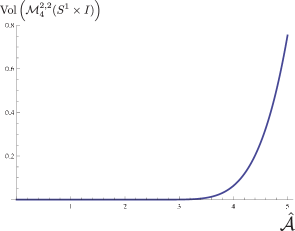
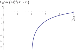
(a)		(b)

Figure 10: (a) The volume of the moduli space of the non-Abelian local vortices on the cylinder $S^{1}\times I$ as a function of the area ${\hat{\mathcal{A}}}$, for $N_{c}=N_{f}=2$ and $k=4$. (b) A logarithmic plot of the volume, showing that the volume vanishes at ${\hat{\mathcal{A}}}=2$ (the Bradlow bound). The volume as a function of ${\hat{\mathcal{A}}}$ differs in the regions ${\hat{\mathcal{A}}}>4$, $3<{\hat{\mathcal{A}}}\leq 4$, $2<{\hat{\mathcal{A}}}\leq 3$ and ${\hat{\mathcal{A}}}<2$ as one approaches the Bradlow bound. The different functions are smoothly connected with each other at the boundaries of each regions up to high derivatives.

So far, we have assumed that the area ${\hat{\mathcal{A}}}$ is sufficiently larger than the vortex charge $k$. However for the fixed vortex charge $k$, there exists an exact lower bound of the area, which is called the Bradlow bound Bradlow:1990ir . The Bradlow bound of the volume essentially comes from the integral formula (4.8), where the integral vanishes if the exponent is negative. So the behavior of the volume changes whether the area is larger than the charge or not. As a result, the functional dependence of the volume on ${\hat{\mathcal{A}}}$ changes as ${\hat{\mathcal{A}}}$ decreases towards the Bradlow bound. For example, let us consider again the case that $N_{c}=N_{f}=2$ (local vortex) and $k=4$ in the limit of $\hat{\varepsilon}\to 0$. As explained, if ${\hat{\mathcal{A}}}$ is larger than 4, the volume is given in (6.13). If $3<{\hat{\mathcal{A}}}\leq 4$, then all the terms containing the factor $({\hat{\mathcal{A}}}-4)$ (in the limit of $\hat{\varepsilon}\to 0$) in (6.11) drop out because of the formula (4.8). Then the volume becomes

$${\rm Vol}\left({\mathcal{M}}^{2,2}_{4}(S^{1}\times I)\right)=\frac{{\hat{\mathcal{A}}}^{8}}{6720}-\frac{{\hat{\mathcal{A}}}^{7}}{252}+\frac{2{\hat{\mathcal{A}}}^{6}}{45}-\frac{4{\hat{\mathcal{A}}}^{5}}{15}+\frac{67{\hat{\mathcal{A}}}^{4}}{72}-\frac{173{\hat{\mathcal{A}}}^{3}}{90}+\frac{409{\hat{\mathcal{A}}}^{2}}{180}-\frac{436{\hat{\mathcal{A}}}}{315}+\frac{1663}{5040}.$$ (6.15)

If $2<{\hat{\mathcal{A}}}\leq 3$, we find similarly

$${\rm Vol}\left({\mathcal{M}}^{2,2}_{4}(S^{1}\times I)\right)=\frac{{\hat{\mathcal{A}}}^{8}}{2880}-\frac{{\hat{\mathcal{A}}}^{7}}{180}+\frac{7{\hat{\mathcal{A}}}^{6}}{180}-\frac{7{\hat{\mathcal{A}}}^{5}}{45}+\frac{7{\hat{\mathcal{A}}}^{4}}{18}-\frac{28{\hat{\mathcal{A}}}^{3}}{45}+\frac{28{\hat{\mathcal{A}}}^{2}}{45}-\frac{16{\hat{\mathcal{A}}}}{45}+\frac{4}{45}.$$ (6.16)

The volume vanishes if ${\hat{\mathcal{A}}}\leq 2$. We plot the volume as a function of ${\hat{\mathcal{A}}}$ for the above regions in Fig. 10. We note that the functions are smoothly connected at each boundary (${\hat{\mathcal{A}}}=3$ and $4$), since the derivatives coincide with each other up to high orders.

7 Conclusion and Discussion

In this paper, we have formulated a path-integral to obtain the volume of the moduli space of the domain-walls. We have seen that the localization method is a powerful tool to calculate the volume of the moduli space without the explicit metric. We have also noticed that the localization method is useful to understand not only the global structure of the moduli space like the volume, but also the detailed and interesting properties of the moduli space through the dualities.

So far, we have not assumed that the supersymmetry is behind the BPS domain-wall system. However, the BRST symmetry, which plays important roles in the localization method, is known to be regarded as a part of the supersymmetry. Actually our BRST transformations (3.1) and (3.2) are the dimensional reduction of the two-dimensional A-twisted supersymmetric transformation to one dimension. So we can expect that our volume formula is closely related to a partition function or vacuum expectation value (vev) in supersymmetric gauge theories. It is interesting to explore non-perturbative corrections in supersymmetric gauge theories from the viewpoint of the volume formula of the moduli space of the BPS domain-walls. When boundaries are present, in particular, not much is known for the non-perturbative corrections in supersymmetric gauge theories. We have found that the boundary conditions are important and determine various interesting properties of the volume calculation. The volume calculation of the moduli space in supersymmetric gauge theories with the boundaries may shed light on the non-perturbative dynamics and dualities.

We have obtained the exact results of the volume of the moduli space by using the localization method, but more directly we can also obtain the volume from an integral of a volume form, constructed by the explicit metric, over the moduli space. The volume is an integral result, where the local information is smeared out, but we can expect that informations on the local metric can be reconstructed from the various uses of the localization method.

We sometimes encounter a mysterious relationship between the BPS solitons and (quantum mechanical) integrable systems like spin chains. The partition functions and vevs in supersymmetric gauge theories often become important quantities in the integrable systems. Our integral formula for the volume of the moduli space, which is expressed in terms of the determinant of the transition matrix, is also reminiscent of the integrable systems. We would like to investigate the relationship between the volume calculation of the BPS solitons and integrable systems in the future.

The volume of the moduli space is also mathematically interesting since the localization method says that the volume is almost determined by a topological nature of the moduli space. The volume of the moduli space may express a topological invariants of the moduli spaces. Recently the localization of the $\mathcal{N}=(2,2)$ supersymmtric gauge theories on $S^{2}$ have been performed Benini:2012ui ; Doroud:2012xw . The partition function of the $\mathcal{N}=(2,2)$ supersymmtric gauge theories has two alternative expressions. One uses the localization around the Higgs branch, where the partition function reduces to the (anti-)vortex moduli zero-modes theory known as the (anti-)vortex partition function Shadchin:2006yz ; Dimofte:2010tz ; Yoshida:2011au ; Miyake:2011yr ; Bonelli:2011fq ; Fujimori:2012ab . The other uses the localization around the Coulomb branch, where the path integral reduces to the multi-contour integrals. These two expressions turn out to be identical. Moreover, it is conjectured in Jockers:2012dk (see also Gomis:2012wy ) that the free energy of the $\mathcal{N}=(2,2)$ supersymmtric gauge theories is the quantum (world sheet instanton) corrected Kähler potential of Kähler moduli for the Higgs branch and actually reproduces the genus-zero Gromov-Witten invariant which counts holomorphic maps from the sphere to the target space manifold.

We have investigated the volume of the moduli space of the vortices on the cylinder via the T-duality. So we can expect that our vortex results on the cylinder may produce the moduli space of novel holomorphic maps from the cylinder to the target manifold.

The width of domain-walls in an infinite interval has been studied in detail. If the mass difference of scalar fields $H$ taking non-vanishing values in the two adjacent vacua is denoted as $\Delta m$, the width of the domain-wall is given by $|\Delta m|/(g^{2}c)$ in the weak coupling region ($g\sqrt{c}\ll|\Delta m|$), but by $1/g\sqrt{c}$ in the strong coupling region ($g\sqrt{c}\gg|\Delta m|$) Kaplunovsky:1998vt ; Eto:2006ng ; Shifman:2002jm . Our results from the localization formula are consistent with the weak coupling result for the infinite interval. Therefore our results suggest that the width of the domain-wall for finite interval does not change significantly as we move from weak coupling toward strong coupling region. Since the effect of boundary is stronger as the length of interval decreases, it is quite possible that the intuition gained from the infinite interval case is not valid for domain-walls in short intervals. It is an interesting future problem to work out the domain-wall solution at finite (short) interval carefully.

We had to guess the sign factors associated with the intersection number of color-lines. We can guess that the sign factor may originate from the fact that our diagonal gauge fixing condition $\Phi^{\alpha}=0$ is ambiguous and ill-defined when eigenvalues $\phi_{a}$ of the matrix $\Phi$ are degenerate. The color-line connecting the boundary conditions at left and right boundaries are usually formulated in terms of eigenvalues of the matrix $\Sigma$, which is canonically conjugate to $\Phi$. This complication is one of the reasons that prevented us to derive more explicitly the sign factors from the precise treatment of path-integral. We leave this question for a future study.

Appendix A Explicit computation of $N_{c}=1$ and $N_{c}=2$ with $N_{f}=3$

Using Eqs. (5.2) and (5.4) for $N_{f}=3$, we find that our localization formula gives

$${\rm Vol}\left({\mathcal{M}}^{1,3}_{1\to 3}\right)=\frac{\beta^{2}}{2}(\hat{L}-d_{13})^{2},$$ (A.1)

$${\rm Vol}\left({\mathcal{M}}^{2,3}_{(1,2)\to(2,3)}\right)=\frac{\beta^{2}}{2}(\hat{L}^{2}-d_{13}^{2}+2d_{12}d_{23}).$$ (A.2)

They differ already at the next-to-leading order in $\hat{L}$.

To check our results of localization formula at non-leading powers of $\hat{L}$, let us compute the volume using the rigid-rod approximation Eto:2007aw where the domain-wall connecting masses $m_{i}$ and $m_{j}$ has a width $d_{ij}$. Let us denote the position of the first (second) wall as $y_{1}$ ($y_{2}$). For the Abelian gauge theory $N_{c}=1$, two walls are non-penetrable Isozumi:2004jc ; Eto:2006ng . Therefore we obtain

$${\rm Vol}\left({\mathcal{M}}^{1,3}_{1\to 3}\right) = \beta^{2}\int_{\frac{d_{12}}{2}}^{\hat{L}-d_{23}-\frac{d_{12}}{2}}dy_{1}\int_{y_{1}+\frac{d_{13}}{2}}^{\hat{L}-\frac{d_{23}}{2}}dy_{2}$$ (A.3)

$$= \frac{\beta^{2}}{2}(\hat{L}-d_{13})^{2},$$

giving an identical result as our localization formula (A.1). For non-Abelian gauge theory $N_{c}=2$, two domain walls are also non-penetrable, but the allowed region of positions are different. We separate the integration region into two and obtain

$${\rm Vol}\left({\mathcal{M}}^{2,3}_{(1,2)\to(2,3)}\right) = \beta^{2}\left(\int_{\frac{d_{23}}{2}+d_{12}}^{\hat{L}-\frac{d_{23}}{2}}dy_{1}\int_{y_{1}-\frac{d_{13}}{2}}^{\hat{L}-\frac{d_{12}}{2}}dy_{2}+\int_{\frac{d_{23}}{2}}^{\frac{d_{23}}{2}+d_{12}}dy_{1}\int_{\frac{d_{12}}{2}}^{\hat{L}-\frac{d_{12}}{2}}dy_{2}\right)$$ (A.4)

$$= \frac{\beta^{2}}{2}(\hat{L}-2d_{12}+d_{13})(\hat{L}-d_{13})+\beta^{2}(L-d_{12})d_{12}$$

$$= \frac{\beta^{2}}{2}(\hat{L}^{2}-d_{13}^{2}+2d_{12}d_{23}),$$

giving an identical result as our localization formula (A.2).

Appendix B Volume of Moduli Space of Dual Non-Abelian Domain Walls

We consider the topological sector with the maximal number of domain walls in $U(N_{c})$ gauge theories with $N_{f}$ flavors of scalar fields in the fundamental representation. The volume of the moduli space of domain walls is given by the determinant of the transition matrix ${\mathcal{T}}^{N_{c},N_{f}}_{(1,\cdots,N_{c})\to(\tilde{N}_{c},\cdots,N_{f})}$ as

$${\rm Vol}\left({\mathcal{M}}^{N_{c},N_{f}}_{(1,\dots,N_{c})\to(\tilde{N}_{c},\cdots,N_{f})}\right)=\beta^{N_{f}}\operatorname{Det}{\mathcal{T}}^{N_{c},N_{f}}_{(1,\cdots,N_{c})\to(\tilde{N}_{c},\cdots,N_{f})}.$$ (B.1)

The leading behavior at large volume is given by the largest powers in $\hat{L}$ as

$$\lim_{\hat{L}\to\infty}\frac{{\mathcal{T}}^{N_{c},N_{f}}_{(1,\cdots,N_{c})\to(\tilde{N}_{c},\cdots,N_{f})}}{\hat{L}^{N_{f}}}=\begin{pmatrix}\frac{1}{\tilde{N}_{c}!}&\cdots&\frac{1}{(N_{c}-2)!}&\frac{1}{(N_{c}-1)!}\\ \vdots&\ddots&\vdots&\vdots\\ \frac{1}{(\tilde{N}_{c}-N_{c}+2)!}&\cdots&\frac{1}{\tilde{N}_{c}!}&\frac{1}{(\tilde{N}_{c}+1)!}\\ \frac{1}{(\tilde{N}_{c}-N_{c}+1)!}&\cdots&\frac{1}{(\tilde{N}_{c}-1)!}&\frac{1}{\tilde{N}_{c}!}\end{pmatrix}.$$ (B.2)

Let us define the determinant of the matrix in the right-hand side as $\Delta^{N_{c},N_{f}}$. For $N_{c}>\tilde{N}_{c}$, the above formula contains factorials of negative integer at the lower left corner. These factorials should be interpreted as zeros

$$\frac{1}{(-n)!}=\frac{1}{\Gamma(-n+1)}=0,\qquad n\in\mathbb{Z}_{+}.$$ (B.3)

In order to obtain the determinant, we subtract the $(N_{c}-1)$-th row multiplied by $\tilde{N}_{c}+1$ from the $N_{c}$-th (last) row of the right-hand side in order to eliminate the right-most entry of the $N_{c}$-th row

$$\Delta^{N_{c},N_{f}}=\operatorname{Det}\begin{pmatrix}\frac{1}{\tilde{N}_{c}!}&\cdots&\frac{1}{(N_{c}-2)!}&\frac{1}{(N_{c}-1)!}\\ \vdots&\ddots&\vdots&\vdots\\ \frac{1}{(\tilde{N}_{c}-N_{c}+2)!}&\cdots&\frac{1}{\tilde{N}_{c}!}&\frac{1}{(\tilde{N}_{c}+1)!}\\ \frac{-(N_{c}-1)}{(\tilde{N}_{c}-N_{c}+1)!}&\cdots&\frac{-1}{(\tilde{N}_{c}-1)!}&0\end{pmatrix}.$$ (B.4)

Similarly subtracting the $(N_{c}-2)$-th row multiplied by $\tilde{N}_{c}+2$ from the $(N_{c}-1)$-th row and continuing the procedure, we can eliminate all the entries of the $N_{c}$-th column except the first row. Thus we find

$$\Delta^{N_{c},N_{f}}=\operatorname{Det}\begin{pmatrix}\frac{1}{\tilde{N}_{c}!}&\cdots&\frac{1}{(N_{c}-2)!}&\frac{1}{(N_{c}-1)!}\\ \frac{-(N_{c}-1)}{(\tilde{N}_{c}-1)!}&\cdots&\frac{-1}{(N_{f}-2)!}&0\\ \vdots&\ddots&\vdots&\vdots\\ \frac{-(N_{c}-1)}{(\tilde{N}_{c}-N_{c}+1)!}&\cdots&\frac{-1}{(\tilde{N}_{c}-1)!}&0\end{pmatrix}.$$ (B.5)

Therefore we obtain the recursion relation

$$\Delta^{N_{c},N_{f}}=\frac{(N_{c}-1)!}{(N_{f}-1)!}\Delta^{N_{c}-1,N_{f}-1}.$$ (B.6)

The recursion relation is solved with the initial condition $\Delta^{1,N_{f}}=1/(N_{f}-1)!$ to give

$$\Delta^{N_{c},N_{f}}=\frac{\prod_{j=1}^{N_{c}}(j-1)!\times\prod_{k=1}^{\tilde{N}_{c}}(k-1)!}{\prod_{i=1}^{N_{f}}(i-1)!}.$$ (B.7)

Thus we find the duality (5.20) is valid. Moreover the coefficient of the leading term is given by the volume of the Grassmann manifold (5.14) apart from the intrinsically ambiguous overall normalization factor to define the moduli space. The proof here is valid also for the leading behavior of the equivalence of Abelian and non-Abelian domain walls, namely agreement between Eqs. (5.5) and (5.6).

References

- (1) N. S. Manton, Nucl. Phys. B 400 (1993) 624.
- (2) P. A. Shah and N. S. Manton, J. Math. Phys. 35 (1994) 1171 [arXiv:hep-th/9307165].
- (3) N. S. Manton and S. M. Nasir, Commun. Math. Phys. 199 (1999) 591 [arXiv:hep-th/9807017].
- (4) S. M. Nasir, Phys. Lett. B 419 (1998) 253 [arXiv:hep-th/9807020].
- (5) N. S. Manton and P. Sutcliffe, “Topological solitons,” Cambridge, UK: Univ. Pr. (2004) 493 p.
- (6) N. A. Nekrasov, Adv. Theor. Math. Phys. 7 (2004) 831 [arXiv:hep-th/0206161].
- (7) G. W. Moore, N. Nekrasov and S. Shatashvili, Commun. Math. Phys. 209 (2000) 97 [arXiv:hep-th/9712241].
- (8) A. A. Gerasimov and S. L. Shatashvili, Commun. Math. Phys. 277 (2008) 323 [arXiv:hep-th/0609024].
- (9) A. Miyake, K. Ohta and N. Sakai, Prog. Theor. Phys. 126 (2012) 637 [arXiv:1105.2087 [hep-th]]; J. Phys. Conf. Ser. 343 (2012) 012107 [arXiv:1111.4333 [hep-th]].
- (10) Y. Isozumi, M. Nitta, K. Ohashi and N. Sakai, Phys. Rev. D 70 (2004) 125014 [hep-th/0405194].
- (11) I. Antoniadis and B. Pioline, Int. J. Mod. Phys. A 12 (1997) 4907 [hep-th/9607058].
- (12) M. Eto, Y. Isozumi, M. Nitta, K. Ohashi, K. Ohta and N. Sakai, Phys. Rev. D 71 (2005) 125006 [hep-th/0412024].
- (13) M. Eto, T. Fujimori, M. Nitta, K. Ohashi, K. Ohta and N. Sakai, Nucl. Phys. B 788 (2008) 120 [hep-th/0703197].
- (14) Y. Isozumi, M. Nitta, K. Ohashi and N. Sakai, Phys. Rev. Lett. 93 (2004) 161601 [hep-th/0404198].
- (15) M. Eto, Y. Isozumi, M. Nitta, K. Ohashi and N. Sakai, hep-th/0607225.
- (16) M. Shifman and A. Yung, Phys. Rev. D 67 (2003) 125007 [hep-th/0212293].
- (17) C. Callias, Commun. Math. Phys. 62, 213 (1978).
- (18) M. F. Atiyah, V. K. Patodi, and I. M. Singer, Math. Proc. Camb. Phil. Soc. 77, 43 (1975).
- (19) I. G. Macdonald, Invent. Math. 56 (1980), 93.
- (20) K. Fujii, J. Appl. Math. 2 (2002), 371-405.
- (21) H. Ooguri and C. Vafa, Nucl. Phys. B 641 (2002) 3 [arXiv:hep-th/0205297].
- (22) M. Eto, T. Fujimori, Y. Isozumi, M. Nitta, K. Ohashi, K. Ohta and N. Sakai, Phys. Rev. D 73 (2006) 085008 [arXiv:hep-th/0601181].
- (23) A. A. Abrikosov, “On The Magnetic Properties Of Superconductors Of The Second Group,” Sov. Phys. JETP 5 (1957) 1174 [Zh. Eksp. Teor. Fiz. 32 (1957) 1442]; H. B. Nielsen and P. Olesen, “Vortex-Line Models For Dual Strings,” Nucl. Phys. B61 (1973) 45.
- (24) M. Eto, T. Fujimori, M. Nitta, K. Ohashi and N. Sakai, Phys. Rev. D 77 (2008) 125008 [arXiv:0802.3135 [hep-th]].
- (25) M. Eto, T. Fujimori, T. Nagashima, M. Nitta, K. Ohashi and N. Sakai, Phys. Lett. B 678 (2009) 254 [arXiv:0903.1518 [hep-th]].
- (26) M. Eto, Y. Isozumi, M. Nitta, K. Ohashi and N. Sakai, Phys. Rev. Lett. 96 (2006) 161601 [hep-th/0511088].
- (27) M. Eto, Y. Isozumi, M. Nitta, K. Ohashi and N. Sakai, J. Phys. A 39 (2006) R315 [hep-th/0602170].
- (28) M. Eto, J. Evslin, K. Konishi, G. Marmorini, M. Nitta, K. Ohashi, W. Vinci and N. Yokoi, Phys. Rev. D 76 (2007) 105002 [arXiv:0704.2218 [hep-th]].
- (29) S. B. Bradlow, Commun. Math. Phys. 135 (1990) 1.
- (30) F. Benini and S. Cremonesi, arXiv:1206.2356 [hep-th].
- (31) N. Doroud, J. Gomis, B. Le Floch and S. Lee, arXiv:1206.2606 [hep-th].
- (32) S. Shadchin, JHEP 0708, 052 (2007)
- (33) T. Dimofte, S. Gukov and L. Hollands, Lett. Math. Phys. 98, 225 (2011)
- (34) Y. Yoshida, arXiv:1101.0872 [hep-th].
- (35) G. Bonelli, A. Tanzini and J. Zhao, JHEP 1206, 178 (2012)
- (36) T. Fujimori, T. Kimura, M. Nitta and K. Ohashi, JHEP 1206, 028 (2012)
- (37) H. Jockers, V. Kumar, J. M. Lapan, D. R. Morrison and M. Romo, arXiv:1208.6244 [hep-th].
- (38) J. Gomis and S. Lee, arXiv:1210.6022 [hep-th].
- (39) V. S. Kaplunovsky, J. Sonnenschein and S. Yankielowicz, Nucl. Phys. B 552 (1999) 209 [hep-th/9811195].