The differential distributions in rapidity and angles of the secondary lepton in the associated production of the top quark pair and higgs boson in proton–proton collisions at the LHC are quite sensitive to the top–higgs coupling. However, the effects of anomalous couplings of the most general $t\bar{t}h$ interaction with operators of dimension-six that are clearly visible in the signal of the associated production of the top quark pair and higgs boson are to large extent obscured by the background sub-processes with the same final state. This means that analyses of such effects, in addition to higher order corrections that are usually calculated for the on-shell top quarks and higgs boson, should include their decays and possibly complete off resonance background contributions to the corresponding exclusive reactions.

1 Introduction.

Associated production of the top quark pair and higgs boson was proposed as a sensitive probe of the top–higgs Yukawa coupling $g_{tth}$ at the $e^{+}e^{-}$ linear collider (LC) [1], [2] more than 20 years ago [3]. A clean experimental environment of the LC seems to be the best place to study the higgs boson profile, including the measurement of $g_{tth}$, but the project of LC is still at the rather early stage of TDR. Fortunately, the top quarks are copiously produced at the LHC that, among others, allows for more and more precise determination of the top quark pair production cross section and for measurements of the cross sections of $t\bar{t}\;+$ jets, see [4] for a review. The measurement of production of $t\bar{t}+b\bar{b}$ [5] is particularly interesting, as it is relevant for observation of the associated production of the top quark pair and higgs boson, with the higgs decaying into $b\bar{b}$. The latter should be the dominant decay mode, if the new boson at a mass of about 125 GeV observed at the LHC [6] is indeed the higgs.

The associated production of the top quark pair and higgs boson in the proton–proton collisions at the LHC

$$pp\;\rightarrow\;t\bar{t}h$$ (1)

is dominated by the gluon–gluon fusion mechanism. Taking into account decays: $h\to b\bar{b}$, $t\to bW^{+}$, $\bar{t}\to\bar{b}W^{+}$ and the subsequent decays of the $W$-bosons, one should consider hard scattering partonic processes as, e.g.,

$$gg\;\rightarrow\;bu\bar{d}\bar{b}\mu^{-}\bar{\nu}_{\mu}b\bar{b},$$ (2)

corresponding to one of the $W$’s decaying hadronically and the other leptonically. Reaction (2) receives contributions from $67\,300$ Feynman diagrams in the leading order of the standard model (SM), in the unitary gauge neglecting masses smaller than $m_{b}$, of which barely 56 diagrams constitute the signal of the $t\bar{t}h$ production and subsequent decay. Some examples of the Feynman diagrams of (2) are shown in Fig. 1. The 56 signal diagrams are obtained from those depicted in Fig. 1(a), 1(b) and 1(c) by attaching the $hb\bar{b}$-vertex to other top or bottom quark lines, interchanging external $b$ and $\bar{b}$ quarks in each of the figures and interchanging the two initial state gluons of Fig. 1(c). The diagrams shown in Fig. 1(d), 1(e) and 1(f) are just a few examples of the background contributions to associated production of the higgs boson and top quark pair.

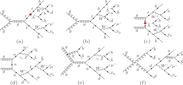
Figure 1: Examples of the lowest order Feynman diagrams of reaction (2): (a), (b) and (c) are the signal diagrams of $t\bar{t}h$ production, (d), (e) and (f) are the $t\bar{t}h$ background contributions. Blobs indicate the higgs–top coupling.

A question arises whether the associated production of the higgs boson and top quark pair can be sensitive to possible modifications of the SM top–higgs Yukawa coupling or not. The question will be addressed in this work by showing how the distributions of the secondary lepton are changed in the presence of such modifications. The distributions computed with the signal diagrams only will be compared with those computed with the full set of the leading order Feynman diagrams that will demonstrate how the background contributions obscure relatively clear effects of the anomalous $t\bar{t}h$ coupling in the signal cross section. Although the issue may seem somewhat premature from the experimental side, but in view of the excellent performance of the LHC, it may become relevant in quite a near future.

2 Calculation details

The calculation is performed in a fully automatic way with a new version [7] of carlomat [8], a general purpose program for Monte Carlo computation of lowest order cross sections. The most general Lagrangian of $t\bar{t}h$ interaction including corrections from dimension-six operators that has been implemented in the program has the following form [9]

$$\mathcal{L}_{t\bar{t}h}=-g_{t\bar{t}h}\bar{t}\left(f+if^{\prime}\gamma_{5}\right)th,$$ (3)

where $g_{t\bar{t}h}=m_{t}/v$, with $v=(\sqrt{2}G_{F})^{-1/2}\simeq 246$ GeV, is the top–higgs Yukawa coupling. The couplings $f$ and $f^{\prime}$ are assumed to be real. They describe, respectively, scalar and pseudoscalar departures from the purely scalar top–higgs Yukawa coupling of SM. The latter is reproduced for $f=1$ and $f^{\prime}=0$. Other dimension-six gauge-invariant effective operators that may have affected the $t\bar{t}h$ interaction are redundant, in a sense that they can be eliminated with the use of the equations of motion, both for the on- and off-shell particles [9]. Obviously, the process of associated production of the higgs boson and top quark pair will be affected by many other possible deviations from the SM couplings. They are not considered here, as the primary goal of the present work is to illustrate just the effects of the anomalous $t\bar{t}h$ interaction on the distributions of the secondary lepton. However, some deviations, eg., the anomalous $Wtb$ coupling generated by the gauge-invariant dimension-six effective operators, which is present in the $t\bar{t}h$ signal diagrams of Figs. 1(a)–(c) and in some off resonance background diagrams such as the one depicted in Fig. 1(d), can be easily included, as it has been already implemented in carlomat. See [10] for the illustration of some effects on the top quark pair production at the LHC that can be caused by the $Wtb$ coupling.

The couplings $f$ and $f^{\prime}$ of Lagrangian (3) belong to least constraint couplings of the SM. For the higgs boson with a mass of 125 GeV, practically the only model independent way to constrain them is to measure the $t\bar{t}h$ production [11]. First results of search for this process in $pp$ collisions at the LHC are reported in [12]. Indirect constraints of the $t\bar{t}h$ interaction vertex can be derived from measurements of the higgs boson production rate through the gluon–gluon fusion process, which is dominated by a top-quark loop, and of the higgs boson decay into 2 photons that, despite being dominated by the $W$ boson loop, also receives a significant contribution from the top-quark loop. However, extraction of the $t\bar{t}h$ coupling in this way relies on the assumption that the loops do not receive contributions from new massive fundamental particles beyond those of the SM. If two universal scale factors are assumed, one for the higgs boson Yukawa couplings to all the SM fermion species and the other for the higgs boson couplings to the EW gauge bosons, and if there is no new physical degrees of freedom, then the scalar coupling $f$ of Eq. (3) can be constraint at 95% C.L. to be in the following regions:

$$f\in[-1.2,-0.6]\cup[0.6,1.3] \qquad{\rm ATLAS}\;\cite[cite]{[\@@bibref{}{fATLAS}{}{}]}$$ (4)

$$f\in[0.3,1.0]\qquad\qquad\qquad\; \qquad{\rm CMS}\;\cite[cite]{[\@@bibref{}{fCMS}{}{}]}.$$ (5)

It should be noted at this point that an opposite sign of the higgs boson coupling to fermions with respect to its coupling to the gauge bosons is required in the Lagrangian for the unitarity and renormalizability of the theory [16] and vacuum stability [17]. Therefore, the interval in the range of negative numbers in (4) is highly disfavoured. The relative sign of both couplings could probably be best determined in the reaction of associated production of the top quark and higgs boson in proton-proton collisions at the LHC through the underlying $t$-channel partonic process $qb\to tq^{\prime}h$ [15].

In carlomat, the on-shell poles in propagators of unstable particles, both the $s$- and $t$-channel ones, are avoided by making the following substitutions:

$$m_{b}^{2}\;\rightarrow\;M_{b}^{2}=m_{b}^{2}-im_{b}\Gamma_{b},\quad b=Z,W,h,\qquad m_{t}\;\rightarrow\;M_{t}=\sqrt{m_{t}^{2}-im_{t}\Gamma_{t}},$$ (6)

where the particle widths are assumed to be constant and the square root with positive real part is chosen, see [8] for details. In order to minimize unitarity violation effects at high energies caused by substitutions (6), which correspond to re-summation of one particle irreducible higher order contributions to $s$-channel propagators, the computation is performed in the complex mass scheme, where the electroweak (EW) couplings are parametrized in terms the complex EW mixing parameter $\sin^{2}\theta_{W}=1-{M_{W}^{2}}/{M_{Z}^{2}}$ which preserves the lowest order Ward identities [18]. Note, that the electric charge $e_{W}$ can be defined as a real quantity in terms of $\alpha_{W}$

$$e_{W}=\sqrt{4\pi\alpha_{W}},\qquad{\rm with}\qquad\alpha_{W}=\frac{\sqrt{2}G_{F}m_{W}^{2}}{\pi}\left(1-\frac{m_{W}^{2}}{m_{Z}^{2}}\right),$$ (7)

as it enters all the EW couplings multiplicatively, which is our choice in the present work. The only effect of using the complex masses of (6) in Eq. (7) would be the overall change of normalization of the cross section. The top–higgs Yukawa coupling is defined in the complex mass scheme by

$$g_{t\bar{t}h}=e_{W}\;\frac{M_{t}}{2\sin\theta_{W}M_{W}},$$ (8)

i.e., it is a complex quantity, as it is parametrized in terms of the complex masses of (6) and complex EW mixing parameter $\sin\theta_{W}$.

3 Results

In this section some results for the differential cross sections and distributions of reaction

$$pp\;\rightarrow\;b\bar{b}bu\bar{d}\bar{b}\mu^{-}\bar{\nu}_{\mu}$$ (9)

at $\sqrt{s}=14$ TeV are presented. For the sake of simplicity and easy reproducibility of the results, only one hard scattering process (2) that dominates at that energy is taken into account. It is folded with CTEQ6L parton distribution functions [19] at the scale $Q=2m_{t}+m_{h}$.

The initial physical input parameters used in the computation are the following. The strong coupling between quarks and gluons is given by $g_{s}=\sqrt{4\pi\alpha_{s}}$, with $\alpha_{s}(m_{Z})=0.118$. The EW couplings are parametrized in terms of the electric charge of (7) that is kept real and the complex EW mixing parameter $\sin\theta_{W}$, as described in Section 2, with the EW gauge boson masses and widths: $m_{W}=80.419$ GeV, $\Gamma_{W}=2.12$ GeV, $m_{Z}=91.1882$ GeV, $\Gamma_{Z}=2.4952$ GeV and the Fermi coupling $G_{F}=1.16639\times 10^{-5}\;{\rm GeV}^{-2}$. The top quark and higgs boson masses are: $m_{t}=173$ GeV, $m_{h}=125$ GeV and their widths that are calculated to the lowest order of SM are the following: $\Gamma_{t}=1.49165$ GeV, $\Gamma_{h}=4.9657$ MeV. The $b$-quark and muon masses are also kept non zero, but their actual values: $m_{b}=4.5\;{\rm GeV}$ and $m_{\mu}=105.65837\;{\rm MeV}$, are numerically irrelevant in practise. Masses of the light quarks of (9) are neglected.

Jets are identified with their original partons and the following cuts on the transverse momenta $p_{T}$, pseudorapidities $\eta$, missing transverse energy $/\!\!\!\!E^{T}$ and separation $\Delta R_{ik}$ in the pseudorapidity–azimuthal angle $(\varphi)$ plane between the objects $i$ and $k$ are imposed:

$$p_{Tl}>30\;{\rm GeV},\qquad p_{Tj}>30\;{\rm GeV},\qquad\left|\eta_{l}\right|<2.1,\qquad\left|\eta_{j}\right|<2.4,$$

$$/\!\!\!\!E^{T}>20\;{\rm GeV},\qquad\Delta R_{lj,jj}=\sqrt{\left(\eta_{i}-\eta_{k}\right)^{2}+\left(\varphi_{i}-\varphi_{k}\right)^{2}}\;>\;0.4,$$ (10)

where the subscripts $l$ and $j$ stand for lepton and jet. Cuts (10) should allow to select events with separate jets, an isolated charged lepton and missing transverse momentum.

Moreover, 100% efficiency of $b$ tagging is assumed and events of the associated production of top quark pair and higgs boson in reaction (9) are selected by imposing the following invariant mass cuts: on the invariant mass of two non $b$ jets, $b_{\sim b_{1}}$ and $b_{\sim b_{2}}$,

$$60\;{\rm GeV}<\left[\left(p_{\sim b_{1}}+p_{\sim b_{2}}\right)^{2}\right]^{1/2}<90\;{\rm GeV},$$ (11)

on the transverse mass of the muon–neutrino system

$$\left[m_{\mu}^{2}+2\left(m_{\mu}^{2}+\left|{\vec{p}}_{\mu}^{\;T}\right|^{2}\right)^{1/2}\left|\;/\!\!\!{\vec{p}}^{\;T}\right|-2{\vec{p}}_{\mu}^{\;T}\cdot/\!\!\!{\vec{p}}^{\;T}\right]^{1/2}<90\;{\rm GeV},$$ (12)

on the invariant mass of a $b$ jet, $b_{1}$, and the two non $b$ jets

$$\left|\left[\left(p_{b_{1}}+p_{\sim b_{1}}+p_{\sim b_{2}}\right)^{2}\right]^{1/2}-m_{t}\right|<30\;{\rm GeV},$$ (13)

on the transverse mass $m_{T}$ of a $b$ quark, $b_{2}$, muon and missing transverse energy

$$m_{t}-30\;{\rm GeV}<m_{T}<m_{t}+10\;{\rm GeV}$$ (14)

and the invariant mass cut on two $b$ jets, $b_{3}$ and $b_{4}$,

$$\left|\left[\left(p_{b_{3}}+p_{b_{4}}\right)^{2}\right]^{1/2}-m_{h}\right|<m_{bb}^{\rm cut},$$ (15)

with either $m_{bb}^{\rm cut}=20$ GeV or, more optimistically, $m_{bb}^{\rm cut}=10$ GeV. In (14), $m_{T}$ is the transverse mass defined by

$$m_{T}^{2}=m^{2}+2\left(m^{2}+\left|{\vec{p}}_{b_{2}}^{\;T}+{\vec{p}}_{\mu}^{\;T}\right|^{2}\right)^{1/2}/\!\!\!\!E^{T}-2\left({\vec{p}}_{b_{2}}^{\;T}+{\vec{p}}_{\mu}^{\;T}\right)\cdot/\!\!\!{\vec{p}}^{\;T},$$

with $m$ being the invariant mass of the $b$-$\mu$ system given by $m^{2}=\left(p_{b_{2}}+p_{\mu}\right)^{2}$. Cuts (11)–(14) should allow to identify the secondary $W$ bosons, the top quarks and the higgs boson. They were used before in the context of the associated production of the top quark pair and higgs boson in $e^{+}e^{-}$ collisions at the LC [20].

For the sake of illustration, the $t\bar{t}h$ couplings of (3) are assigned the following values: $f=1,0$ and $f^{\prime}=0,\pm 1$ and the differential distributions of the final state muon, generally referred to as lepton, of reaction (9) are computed, first with the 56 signal Feynman diagrams of the associated production of the top quark pair and higgs boson and then with the complete set of $67\,300$ Feynman diagrams, as discussed in Section 1. The rapidity and angular differential cross sections and distributions of the lepton for which the effects of anomalous couplings are best visible will be shown in Figs. 3–6 and the distributions in the lepton transverse momentum or energy which are practically not affected by the couplings will not be presented.

The size of background contributions to the associated production of the higgs boson and top quark pair in $pp$ collisions at $\sqrt{s}=14$ TeV is illustrated in Fig. 2, where the differential cross sections of (9) are plotted as functions of the muon rapidity, $y_{l}$, cosine of the muon angle with respect to beam, $\cos\theta_{l{\rm b}}$ and cosine of the muon angle with respect to the reconstructed higgs boson momentum, $\cos\theta_{lh}$. The cross sections plotted in Fig. 2 have been computed with different cuts. In the left and central panel, the boxes shaded in light grey show the cross sections computed with cuts (10) and the grey boxes depict the cross sections calculated with cuts (10) and the invariant mass cuts (11)–(14). These results are not shown in the right panel of Fig. 2, as it is in principle not possible to reconstruct the higgs boson momentum without cut (15) on its invariant mass. The short-dashed (dotted) lines show the results for $m_{bb}^{\rm cut}=20$ GeV ($m_{bb}^{\rm cut}=10$ GeV) and the solid line in each panel of Fig 2 shows the results for the signal cross section calculated with $m_{bb}^{\rm cut}=20$ GeV. It should be noted here that the signal cross section is fairly independent of $m_{bb}^{\rm cut}$. As can be seen, the background is quite large and decreasing a value of $m_{bb}^{\rm cut}$ seems to be a right way towards its reduction.

Distributions in 3 different kinematical variables of the final state lepton of (9): rapidity, $y_{l}$, cosine of the angle with respect to the beam, $\cos\theta_{l{\rm b}}$ and cosine of the angle with respect to the reconstructed higgs boson momentum, $\cos\theta_{lh}$ are shown in Figs. 3–5. In each of the figures, the left panels show the $t\bar{t}h$ production signal, computed with 56 Feynman diagrams, and the right panels show the complete leading order predictions, computed with $67\,300$ Feynman diagrams. The grey boxes show the corresponding SM results, i.e. the results obtained with $f=1$ and $f^{\prime}=0$. Cuts (10)–(14) and (15) with $m_{bb}^{\rm cut}=20$ GeV are applied to all the distributions presented. A relatively clear effect of the anomalous couplings $f$ and $f^{\prime}$ that can be seen in the $t\bar{t}h$ signal distributions on the left hand side of all Figs. 3–6 is to large extent obscured by the background contributions in the plots on the right hand side which show the full leading order results.

In order to illustrate what a role invariant mass cuts (10)–(15) play, the distributions of the final state lepton of (9) at $\sqrt{s}=14$ TeV in $y_{l}$ and $\cos\theta_{l{\rm b}}$ with different cuts are compared in Fig. 6. The left panels show the distributions with the cuts given by (10) and the right panels show the distributions with cuts (10)–(14) and (15) with $m_{bb}^{\rm cut}=10$ GeV for two different combinations of the scalar and pseudoscalar $t\bar{t}h$ couplings of (3). Again the grey boxes show the SM results. Although the invariant mass cuts suppress the background contributions to some extent, the degree of suppression does not look very satisfactory.

Figure 2: The differential cross sections of (9) at $\sqrt{s}=14$ TeV as functions of the muon rapidity $y_{l}$, cosine of the muon angle with respect to beam $\cos\theta_{l{\rm b}}$ and cosine of the muon angle with respect to the higgs boson $\cos\theta_{lh}$ computed with different cuts as described in the main text.

Figure 3: Distributions in rapidity of the final state lepton of (9) in $pp$ collisions at $\sqrt{s}=14$ TeV with different combinations of the scalar and pseudoscalar $t\bar{t}h$ couplings: $t\bar{t}h$ production signal (left panels) and complete leading order prediction (right panels).

Figure 4: Distributions in cosine of the angle between the final state lepton of (9) with respect to the beam in $pp$ collisions at $\sqrt{s}=14$ TeV with different combinations of the scalar and pseudoscalar $t\bar{t}h$ couplings: $t\bar{t}h$ production signal (left panels) and complete leading order prediction (right panels).

Figure 5: Distributions in cosine of the angle between the final state lepton of (9) and the higgs boson in $pp$ collisions at $\sqrt{s}=14$ TeV with different combinations of the scalar and pseudoscalar $t\bar{t}h$ couplings: $t\bar{t}h$ production signal (left panels) and complete leading order prediction (right panels).

Figure 6: Distributions of the final state lepton of (9) at $\sqrt{s}=14$ TeV in $y_{l}$ and $\cos\theta_{l{\rm b}}$ with the cuts given by (10) (left panels) and (10)–(14) and (15) with $m_{bb}^{\rm cut}=10$ GeV (right panels) for different combinations of the scalar and pseudoscalar $t\bar{t}h$ couplings.

The signal significance $\mu=\sigma(f,f^{\prime})/\sigma_{SM}$ and corresponding differences in expected numbers of events, $\Delta n=n(f,f^{\prime})-n_{SM}$, for different combinations of the couplings $(f,f^{\prime})$, with the $\mu^{-}$ in the forward $(\cos\theta_{lh}>0)$ or backward $(\cos\theta_{lh}<0)$ hemisphere with respect to the direction of the higgs boson, in reaction (9) at $\sqrt{s}=14$ TeV are shown in Table 1. The cuts are given by (10)–(15) with $m_{bb}^{\rm cut}=20$ GeV (columns 2–5) and $m_{bb}^{\rm cut}=10$ GeV (columns 6–9). The event numbers have been calculated assuming an integrated luminosity of $100~{}{\rm fb}^{-1}$ and 100% detection efficiency. Therefore, they should be treated with care, in particular because of the fact that only the leading order contributions to reaction (9) are taken into account. However, the leading order predictions for signal significance $\mu$ are more reliable. In particular, $\mu\approx 1.2$ for $f=1$ and $|f^{\prime}|=1$ indicates a potential of the reaction of associated production of the higgs boson and top quark pair in obtaining direct limits on the pseudoscalar coupling $f^{\prime}$. If only the $t\bar{t}h$ signal contributions to the cross section are taken into account, then the signal significance for this particular combination of couplings becomes even bigger, amounting to $\mu=1.4$ in the forward and $\mu=1.6$ in the backward hemisphere with respect to the direction of the higgs boson. This again shows how the off resonance background contributions obscure the signal of $t\bar{t}h$ production.

	$m_{bb}^{\rm cut}=20$ GeV				$m_{bb}^{\rm cut}=10$ GeV
	$\cos\theta_{lh}<0$		$\cos\theta_{lh}>0$		$\cos\theta_{lh}<0$		$\cos\theta_{lh}>0$
$(f,f^{\prime})$	$\mu\;\;$	$\Delta n$	$\mu\;\;$	$\Delta n$	$\mu\;\;$	$\Delta n$	$\mu\;\;$	$\Delta n$
$(0,1)$	0.90	$-148$	0.83	$-265$	0.85	$-174$	0.78	$-275$
$(0,-1)$	0.90	$-151$	0.84	$-252$	0.84	$-188$	0.78	$-270$
$(1,1)$	1.20	295	1.17	251	1.23	261	1.17	210
$(1,-1)$	1.20	302	1.15	238	1.24	279	1.18	221

Table 1: The signal significance $\mu$ and corresponding difference in numbers of events $\Delta n$ for different combinations of the couplings $(f,f^{\prime})$ in reaction (9) at $\sqrt{s}=14$ TeV.

4 Summary and conclusions

The differential cross sections and distributions of the final state lepton of (9) in rapidity, cosine of its angle with respect to the beam and cosine of its angle with respect to the reconstructed higgs boson momentum have been computed to the leading order in the presence of most general $t\bar{t}h$ interaction with operators of dimension-six. The distributions computed with the $t\bar{t}h$ signal diagrams only, which are substantially changed in the presence of anomalous $t\bar{t}h$ couplings, have been compared with those computed with the full set of the leading order Feynman diagrams. The comparison have shown that the background contributions to large extent obscure the relatively clear effects of the anomalous $t\bar{t}h$ coupling in the signal distributions. This means that analyses of such effects [21], in addition to higher order corrections [22] that are usually calculated for the on-shell top quarks and higgs boson, should include their decays and possibly complete off resonance background contributions to the corresponding exclusive reactions. The only reasonable way to make the effects of anomalous couplings better visible seems to be imposing more and more restrictive cuts.

Acknowledgements: This project was supported in part with financial resources of the Polish National Science Centre (NCN) under grant decision number DEC-2011/03/B/ST6/01615 and by the Research Executive Agency (REA) of the European Union under the Grant Agreement number PITN-GA-2010-264564 (LHCPhenoNet).

References

-
[1]
James Brau, Yasuhiro Okada, Nicholas Walker, et al.
[ILC Reference Design Report Volume 1 - Executive Summary],
arXiv:0712.1950;
J.A. Aguilar-Saavedra et al. [ECFA/DESY LC Physics Working Group Collaboration], arXiv:hep-ph/0106315;
T. Abe et al., [American Linear Collider Working Group Collaboration], arXiv:hep-ex/0106056;
K. Abe et al. [ACFA Linear Collider Working Group Collaboration], arXiv:hep-ph/0109166. - [2] CLIC Study <http://clic-study.web.cern.ch/clic-study/>.
-
[3]
A. Djouadi, J. Kalinowski, P.M. Zerwas,
Mod. Phys. Lett. A7 (1992) 1765;
A. Djouadi, J. Kalinowski, P.M. Zerwas, Z. Phys C54 (1992) 255. - [4] F.-P. Schilling, Int. J. Mod. Phys. A27 (2012) 1230016 [arXiv:1206.4484].
- [5] CMS Collaboration, First Measurement of the Cross Section Ratio in pp Collisions at TeV, CMS-PAS-TOP-12-024 (2012).
-
[6]
ATLAS Collaboration, Phys. Lett. B716 (2012) 1;
CMS Collaboration, Phys. Lett. B716 (2012) 30. - [7] K. Kołodziej, arXiv:1305.5096. Program available from: http://kk.us.edu.pl/.
-
[8]
K. Kołodziej, Comput. Phys. Commun. 180 (2009)
1671;
K. Kołodziej, Acta Phys. Polon. B42 (2011) 2477. - [9] J.A. Aguilar-Saavedra, Nucl. Phys. B821 (2009) 215 [arXiv:0904.2387].
- [10] K. Kołodziej, arXiv:1212.6733.
-
[11]
F. Maltoni, D. L. Rainwater, S. Willenbrock,
Phys. Rev. D66 (2002) 034022, [arXiv:hep-ph/0202205];
A. Belyaev, L. Reina, JHEP 08 (2002) 041, [arXiv:hep-ph/0205270]. - [12] CMS Collaboration, CMS-HIG-12-035, CERN-PH-EP-2013-027, arXiv:1303.0763, submitted to JHEP.
- [13] ATLAS Collaboration, Combined coupling measurements of the Higgs-like boson with the ATLAS detector using up to of proton-proton collision data, ATLAS-CONF-2013-034, March 13, 2013.
- [14] CMS Collaboration, Observation of a resonance with a mass near 125 GeV in the search for the Higgs boson in collisions at TeV and 8 TeV, CMS-PAS-HIG-12-020, July 2012.
-
[15]
S. Biswas, E. Gabrielli, B. Mele, JHEP 1301 (2013) 088;
S. Biswas, E. Gabrielli, F. Margaroli, B. Mele, arXiv:1304.1822. - [16] T. Appelquist, M. S. Chanowitz, Phys. Rev. Lett. 59 (1987) 2405 [Erratum-ibid. 60 (1988) 1589].
- [17] M. Reece, arXiv:1208.1765.
- [18] A. Denner, S. Dittmaier, M. Roth, D. Wackeroth, Nucl. Phys. B560 (1999) 33 and Comput. Phys. Commun. 153 (2003) 462.
- [19] J. Pumplin et al., JHEP 07 (2002) 012.
-
[20]
K. Kołodziej, S. Szczypiński, Nucl. Phys. B801 (2008)
153, [arXiv:0803.0887];
K. Kołodziej, S. Szczypiński, Eur. Phys. J. C64 (2009) 645 [arXiv:0903.4606]. - [21] C. Degrande, J.M. Gerard, C. Grojean, F. Maltoni, G. Servant, JHEP 1207 (2012) 036, Erratum-ibid. 1303 (2013) 032.
- [22] P. Baernreuther, M. Czakon, A. Mitov, Phys. Rev. Lett. 109 (2012) 132001 [arXiv:1204.5201].