C nicas y Superficies Cu dricas

Abstract.

There are two problems Analytical Geometry with facing anyone who studies this discipline: define the nature of the locus represented by the general equation $2^{do}$ degree in two or three variables:
That curve represents the plane?
What surface is in space?
These two problems are posed and solved by applying the study of matrices and spectral theory.

1. Introducci n

Hay en la Geometr a Anal tica dos problemas con los que se enfrenta todo el que estudie sta disciplina:
definir la naturaleza del Lugar Geom trico representado por la ecuaci n general de $2^{do}$ grado en dos o tres variables. Por ejemplo,

1. donde la ecuaci n $3x^{2}-2xy+y^{2}-x+y+5=0,$ ¿Que curva representa en el plano? y
   

2. donde la ecuaci n $x^{2}+2y^{2}-5z^{2}+2xy+3xz-4yz+2x+3y-5z+8=0,$ ¿Qu superficie representa en el espacio?

La respuesta en el primer caso es que la curva es una c nica (elipse, par bola, hip rbola) una c nica degenerada y en el segundo caso es una superficie cu drica (cono, cilindro, elipsoide, paraboloide,…) un caso degenerado de ellas.
En el $1^{er}$ caso es posible estudiar el problema con elementos que proporciona la Trigonometr a empleando funciones del ngulo doble para definir el $\measuredangle$ que deben girarse los ejes para conseguir anular el t rmino mixto.
Pero para estudiar el segundo problema es imprescindible el empleo de las matrices y los valores propios junto con el Teorema Espectral para matrices sim tricas.
Estos dos problemas ser n planteados y resueltos aplicando, como ya se dijo, las matrices y la teor a espectral que acaba de estudiarse en los dos cap tulos anteriores.

2. Lugares geom tricos representados por la ecuaci n general de segundo grado en dos variables: $Ax^{2}+2Bxy+Cy^{2}+2Dx+2Ey+F=0$

El problema que vamos a abordar es el siguiente: dada la ecuaci n

(1) $$Ax^{2}+2Bxy+Cy^{2}+2Dx+2Ey+F=0$$

donde $A,B,C,D,E,F$ son constantes reales dadas, ¿Qu conjunto de puntos del plano $xy$ la satisfacen?
La ecuaci n [1]:

• Una componente cuadr tica:

  $$Ax^{2}+2Bxy+Cy^{2}=\left(\begin{array}[]{cc}x&y\end{array}\right)\left(\begin{array}[]{cc}A&B\\ B&C\end{array}\right)\left(\begin{array}[]{c}x\\ y\end{array}\right)$$

• Una componente lineal:

  $$2Dx+2Ey=\left(\begin{array}[]{cc}2D&2E\end{array}\right)\left(\begin{array}[]{c}x\\ y\end{array}\right)$$

• Un t rmino independiente:

  $$F$$

Asumiremos que No todos los coeficientes $A,B,C$ de la componente cuadr tica se anulan, ya que si as fuese, [1] representar a la recta del plano

$$2Dx+2Ey+F=0$$

y no hay nada que analizar.
Como se desprender del estudio que vamos a hacer, la ecuaci n [1] puede representar:

$$\text{Una c nica}\begin{cases}\text{Circunferencia}\\ \text{Elipse}\\ \text{Hip rbola}\\ \text{Par bola}\end{cases}$$

O una

$$\text{c nica degenerada}\begin{cases}\text{dos rectas paralelas}\\ \text{dos rectas concurrentes}\\ \text{una recta}\\ \text{un punto}\\ \emptyset\mathchar 46\relax\,\,\text{O sea que\,\, $\nexists(x,y)\in\mathbb{R}^{2}$\,\, que satisfagan [\ref{1}]}\end{cases}$$

todo depender , en el fondo, de los invariantes de [1] y de los valores propios de la matriz

$$M=\left(\begin{array}[]{cc}A&B\\ B&C\end{array}\right)$$

Llamaremos en adelante c nica al lugar geom trico representado por [1], o sea, el conjunto de puntos del plano que satisfacen [1].
Consideremos, pues, la c nica [1]. Reducirla es definir el lugar geom trico representado por la ecuaci n.
Asosiado a [1] hay dos funciones:

$q$ es la f.c (forma cuadr tica) asociada a [1]

1. $$f :\mathbb{R}^{2}\longrightarrow\mathbb{R}$$

   $$(x,y)\longrightarrow f(x,y)=q(x,y)+\left(2D\,\,2E\right)\dbinom{x}{y}+F$$

El Kernel de $f$ (o el n cleo de $f$) es el conjunto

$$\ker f=f^{-1}({0})=\left\{(x,y)\diagup f(x,y)=0\right\}\mathchar 46\relax$$

La c nica [1] no es m s que el $\ker f$. Adem s es claro que un punto $P(x,y)$ est en la c nica   $\Longleftrightarrow f(x,y)=0\Longleftrightarrow q(x,y)+\left(2D\,\,2E\right)\dbinom{x}{y}+F=0\mathchar 46\relax$
Notese adem s que

$$\dfrac{\partial f}{\partial x} =2Ax+2By+2D$$

$$\dfrac{\partial f}{\partial y} =2Bx+2Cy+2E$$

La naturaleza del lugar representado por [1] est ntimamente ligada a ciertos escalares que se construyen con los coeficientes de la matriz sim trica

$$\left(\begin{array}[]{ccc}A&B&D\\ B&C&E\\ D&E&F\end{array}\right)$$

Ello son:

$$\Delta=\left|\begin{array}[]{ccc}A&B&D\\ B&C&E\\ D&E&F\end{array}\right|=ACF-AE^{2}-B^{2}F+2BDE-CD^{2}\mathchar 46\relax$$

$\Delta$ es llamado el invariante c bico de [1] el discriminante de la c nica.

$$\delta=\left|\begin{array}[]{cc}A&B\\ B&C\end{array}\right|=AC-B^{2}=M_{33}$$

$M_{33}:$ menor principal $3-3$ de la matriz

(2) $$\left(\begin{array}[]{ccc}A&B&D\\ B&C&E\\ D&E&F\end{array}\right)$$

$\delta$ es llamado el invariante cuadr tico lineal de [1].
$\omega=A+C;$ $\omega$ es llamado el invariante linaeal de [1].
Estos escalares se llaman los invariantes de la c nica porque son cantidades que como se ver no cambian de valor cuando sometemos [1] bien sea a una trasposici n una rotaci n de ejes. Los menores principales de orden dos de [2] son:

$$M_{11}=\left|\begin{array}[]{cc}C&E\\ E&F\end{array}\right|;\hskip 14.22636ptM_{22}=\left|\begin{array}[]{cc}A&D\\ D&F\end{array}\right|;\hskip 14.22636ptM_{33}=\delta=\left|\begin{array}[]{cc}A&B\\ B&C\end{array}\right|$$

De los tres, solo $M_{33}$ es invariante. Estos tres menores, sobre todo $\delta=M_{33}$, van a ser importantes en el problema de la reducci n de la c nica.

Ejemplo 2.1.

1. Un caso en que el lugar es $\emptyset\mathchar 46\relax$
   

   $$f(x,y)=x^{2}+y^{2}-4x-6y+24=0$$

   Para identificar el lugar tratemos de completar trinomios cuadrados perfectos.
   

   $$f(x,y) =\left(x^{2}-4x+4\right)+\left(y^{2}-6y+9\right)+24-13$$

   $$={\left(x-2\right)}^{2}+{\left(y-3\right)}^{2}+11=0$$

$$\nexists(x,y)\in\mathbb{R}^{2}\hskip 14.22636pt\text{t.q}\hskip 14.22636ptf(x,y)=0\mathchar 46\relax$$

El lugar es $\emptyset$.

Sea $f(x,y)=x^{2}+y^{2}-4x-6y+13=0\mathchar 46\relax$ Entonces

$$f(x,y) =\left(x^{2}-4x+4\right)+\left(y^{2}-6y+9\right)+\cancel{13}-\cancel{13}$$

$$={\left(x-2\right)}^{2}+{\left(y-3\right)}^{2}=0\mathchar 46\relax$$

El nico punto que satisface $f(x,y)=0$ es (2,3).
As que el lugar es un punto.

Dos rectas paralelas.
Sean

(3) $$l(x,y)=3x-2y+2=0$$

(4) $$m(x,y)=3x-2y+1=0$$

Definamos

$$f(x,y) =l(x,y)\cdot m(x,y)$$

$$=\left(3x-2y+2\right)\left(3x-2y+1\right)$$

(5) $$=9x^{2}-12xy+4y^{2}+9x-6y+2=0$$

Es claro que

$$f(x,y) =0\Longleftrightarrow l(x,y)\cdot m(x,y)=0$$

$$\Longleftrightarrow l(x,y)=0\hskip 14.22636pt\text{ }\hskip 14.22636ptm(x,y)=0$$

$$\Longleftrightarrow(x,y)\hskip 14.22636pt\text{est en la recta [\ref{3}] en la recta [\ref{4}]}$$

Luego el lugar representado por [5] consta de dos rectas paralelas.

Dos rectas que se cortan.
Sean

(6) $$l(x,y)=3x-2y+1=0$$

(7) $$m(x,y)=x+y-2=0$$

[6] y [7] representan dos rectas que se cortan.
Definamos

$$f(x,y) =l(x,y)\cdot m(x,y)$$

$$=\left(3x-2y+1\right)\left(x+y-2\right)$$

(8) $$=3x^{2}+xy-2y^{2}-5x+5y-2=0$$

Es claro que

$$f(x,y) =0\Longleftrightarrow l(x,y)\cdot m(x,y)=0$$

$$\Longleftrightarrow l(x,y)=0\hskip 14.22636pt\text{ }\hskip 14.22636ptm(x,y)=0$$

$$\Longleftrightarrow(x,y)\hskip 14.22636pt\text{est en la recta [\ref{6}] en la recta [\ref{7}]}$$

El lugar r presentado por [8] consta de dos rectas que se cortan.

Una recta.
Sea

$$l(x,y)=x+y-2=0$$

Definamos

$$f(x,y) =l(x,y)\cdot l(x,y)=\left(x+y-2\right)\left(x+y-2\right)$$

(9) $$=x^{2}+2xy+y^{2}-4x-4y+4=0$$

Es claro que

$$f(x,y)=0\Longleftrightarrow l(x,y)=x+y-2=0$$

El lugar representado por [9] es una recta.

3. Invariantes de una c nica

Proposición 3.1.

Consideremos la c nica de la ecuaci n [1]. Los n meros reales

$$\omega=A+C,\hskip 14.22636pt\delta=\left|\begin{array}[]{cc}A&B\\ B&C\end{array}\right|=AC-B^{2}\hskip 14.22636pt\text{y}\hskip 14.22636pt\Delta=\left|\begin{array}[]{ccc}A&B&C\\ B&C&E\\ D&E&F\end{array}\right|$$

no cambian al realizar una traslaci n, una rotaci n de los ejes $xy$, o una combinaci n de ambas transformaciones.

Demostración.

1. Supongamos que realizamos una traslaci n de los ejes xy al punto $O^{\prime}(h,k)$. (Fig.1.1). Entonces se definen ejes X-Y con origen en O’y paralelos a x-y teniendose que

   $$x =X+h$$

   $$y =Y+k$$

   que llevamos a [1] obteniendose

   

   Figura 1.

   $$A{\left(X+h\right)}^{2}+2B\left(X+h\right)\left(Y+k\right)+C{\left(Y+k\right)}^{2}+2D\left(X+h\right)+2E\left(Y+k\right)+F=0$$

   O sea que
   $AX^{2}+2BXY+CY^{2}+2\left(Ah+Bk+D\right)X+2\left(Bh+Ck+E\right)Y+\left(Ah^{2}+2Bhk+Ck^{2}+2Dh+2Ek+F\right)=0$
   ecuaci n que podemos escribir en la forma

   $$A^{\prime}X^{2}+2B^{\prime}XY+C^{\prime}Y^{2}+2D^{\prime}X+2E^{\prime}Y+F^{\prime}=0\hskip 14.22636pt\text{siendo}$$

   $$A^{\prime}=A$$

   $$B^{\prime}=B$$

   $$C^{\prime}=C$$

   $$D^{\prime}=Ah+Bk+D=\dfrac{1}{2}\left\mathchar 46\relax\dfrac{\partial f}{\partial x}\right)_{h,k}$$

   $$E^{\prime}=Bh+Ck+E=\dfrac{1}{2}\left\mathchar 46\relax\dfrac{\partial f}{\partial y}\right)_{h,k}$$

   $$F^{\prime}=Ah^{2}+2Bhk+Ck^{2}+2Dh+2Ek+F=f(h,k)$$

   N tese que cuando se hace una traslaci n de ejes al punto $(h,k)$ los coeficientes de la parte cuadr tica de la ecuaci n no se tranasforman.
   Si lo hacen los coeficientes de la parte lineal y el t rmino independiente que ahora es $f(h,k)$.
   En imagenes.

   

   nueva componente lineal:$\left(\begin{array}[]{cc}2\left(Ah+Bk+D\right)&2\left(Bh+Ck+E\right)\end{array}\right)\left(\begin{array}[]{cc}X\\ Y\end{array}\right)$
   nuevo t rmino independiente: $f(h,k)=\left(\begin{array}[]{cc}h&k\end{array}\right)\left(\begin{array}[]{cc}A&B\\ B&C\end{array}\right)\left(\begin{array}[]{cc}h\\ k\end{array}\right)+\left(\begin{array}[]{cc}2D&2E\end{array}\right)\left(\begin{array}[]{cc}h\\ k\end{array}\right)+F$ Calculemos los nuevos valores de $\omega,\delta,$ y $\Delta$.
   

   $$\omega^{\prime} =A^{\prime}+C^{\prime}=A+C=\omega$$

   $$\delta^{\prime} =\left|\begin{array}[]{cc}A^{\prime}&B^{\prime}\\ B^{\prime}&C^{\prime}\end{array}\right|=\left|\begin{array}[]{cc}A&B\\ B&C\end{array}\right|=AC-B^{2}=\delta\mathchar 46\relax$$

   Esto demuestra que $\omega$ y $\delta$ son invariantes por traslaci n.
   Veamos ahora que $\Delta$ tambi n se conserva.

   $$\Delta^{\prime} =\left|\begin{array}[]{ccc}A^{\prime}&B^{\prime}&D^{\prime}\\ B^{\prime}&C^{\prime}&E^{\prime}\\ D^{\prime}&E^{\prime}&F^{\prime}\end{array}\right|$$

   $$=\left|\begin{array}[]{cccc}A&B&Ah+Bk+D\\ B&C&Bh+Ck+E\\ Ah+Bk+D&Bh+Ck+E&Ah^{2}+2Bhk+Ck^{2}+2Dh+2Dh+2Ek+F\end{array}\right|$$

   $$\underset{\tiny f_{3}\rightarrow f_{3}-hf_{1}-kf_{2}}{\underset{\uparrow}{=}}\left|\begin{array}[]{cccc}A&B&Ah+Bk+D\\ B&C&Bh+Ck+E\\ D&E&Dh+Ek+F\end{array}\right|\underset{\tiny c_{3}\rightarrow c_{3}-hc_{1}-kc_{2}}{\underset{\uparrow}{=}}\left|\begin{array}[]{cccc}A&B&C\\ B&C&E\\ D&E&F\end{array}\right|=\Delta$$

   lo que nos demuestra que $\Delta$ tambi n es invariante por traslaci n.

2. Supongamos ahora que rotamos los ejes $xy$ un ngulo $\overset{\curvearrowleft}{\theta}(0<\theta<\phi/2)$ respecto a $O$.

   

   Figura 2.

   Se obtiene as un nuevo sistema $XY$ con origen en $O$.
   Llamemos $\vec{P_{1}}$ y $\vec{P_{2}}$ a los vectores unitarios que se alan las dimensiones de los nuevos ejes. Sea $Q$ un punto cualquiera del plano de vector de posici n $\vec{r}$ respecto a $O$.
   

   $$\left[\vec{r}\right]_{e_{\alpha}}=\left[I\right]_{e_{\alpha}}^{p_{\alpha}}\left[\vec{r}\right]_{p_{\alpha}}$$

   O sea

   $$\left(\begin{array}[]{cc}x\\ y\end{array}\right)=\left(\begin{array}[]{cc}\cos\theta&-\sin\theta\\ \sin\theta&\cos\theta\end{array}\right)\left(\begin{array}[]{cc}X\\ Y\end{array}\right)=P\left(\begin{array}[]{cc}X\\ Y\end{array}\right)$$

   con

   $$P=\left(\begin{array}[]{cc}\cos\theta&-\sin\theta\\ \sin\theta&\cos\theta\end{array}\right):\text{ortogonal}$$

   La c nica referida a los ejes $xy$ tiene por ecuaci n:

   $$\left(\begin{array}[]{cc}x&y\end{array}\right)\left(\begin{array}[]{cc}A&B\\ B&C\end{array}\right)\left(\begin{array}[]{cc}x\\ y\end{array}\right)+\left(\begin{array}[]{cc}2D&2E\end{array}\right)\left(\begin{array}[]{cc}x\\ y\end{array}\right)+F=0$$

   Pero

   $$\left(\begin{array}[]{cc}x\\ y\end{array}\right)=P\left(\begin{array}[]{cc}X\\ Y\end{array}\right)$$

   y al transponer,

   $$\left(\begin{array}[]{cc}x&y\end{array}\right)=\left(\begin{array}[]{cc}X&Y\end{array}\right)P^{t}\mathchar 46\relax$$

   Luego

   $$\left(\begin{array}[]{cc}X&Y\end{array}\right)\left(P^{t}\left(\begin{array}[]{cc}A&B\\ B&C\end{array}\right)P\right)\left(\begin{array}[]{cc}X\\ Y\end{array}\right)+\left(\begin{array}[]{cc}2D&2E\end{array}\right)P\left(\begin{array}[]{cc}X\\ Y\end{array}\right)+F=0$$

   es la ecuaci n de c nica $\diagup XY\mathchar 46\relax$
   N tese que

   $$P^{t}\left(\begin{array}[]{cc}A&B\\ B&C\end{array}\right)P$$

   es sim trica ya que

   $${\left(P^{t}\left(\begin{array}[]{cc}A&B\\ B&C\end{array}\right)P\right)}^{t}=P^{t}\left(\begin{array}[]{cc}A&B\\ B&C\end{array}\right)P$$

   Si llamamos

   $$\left\mathchar 46\relax\begin{split}\left(\begin{array}[]{cc}A^{\prime}&B^{\prime}\\ B^{\prime}&C^{\prime}\end{array}\right)&=P^{t}\left(\begin{array}[]{cc}A&B\\ B&C\end{array}\right)P\\ \text{y}\hskip 14.22636pt\left(\begin{array}[]{cc}2D^{\prime}&2E^{\prime}\end{array}\right)&=\left(\begin{array}[]{cc}2D&2E\end{array}\right)P\end{split}\right\}\hskip 14.22636pt\star$$

   se tiene que

   $$\left(\begin{array}[]{cc}A^{\prime}&B^{\prime}\\ B^{\prime}&C^{\prime}\end{array}\right)$$

   es sim trica y la ecuaci n de la c nica $\diagup XY$ es:

   $$\left(\begin{array}[]{cc}X&Y\end{array}\right)\left(\begin{array}[]{cc}A^{\prime}&B^{\prime}\\ B^{\prime}&C^{\prime}\end{array}\right)\left(\begin{array}[]{cc}X\\ Y\end{array}\right)+\left(\begin{array}[]{cc}2D&2E\end{array}\right)\left(\begin{array}[]{cc}X\\ Y\end{array}\right)+F=0,$$

   o tambi n,

   $$A^{\prime}X^{2}+2B^{\prime}XY+C^{\prime}Y^{2}+2D^{\prime}X+2E^{\prime}Y+F=0$$

   donde $A^{\prime},B^{\prime},C^{\prime},D^{\prime},E^{\prime}$ se calculan utilizando $\star$.
   Observese que cuando realizamos una rotaci n de ejes, tanto la parte cuadr tica como la parte lineal se transforman. El t tmino independiente no se afecta.
   En im genes:

   

   
   

   Los nuevos valores de $\omega,\delta$ y $\Delta$ son ahora:

   $$\omega^{\prime} =A^{\prime}+C^{\prime}$$

   $$\delta^{\prime} =\left|\begin{array}[]{cc}A^{\prime}&B^{\prime}\\ B^{\prime}&C^{\prime}\end{array}\right|=A^{\prime}C^{\prime}-B^{\prime 2}$$

   $$\Delta^{\prime} =\left|\begin{array}[]{ccc}A^{\prime}&B^{\prime}&C^{\prime}\\ B^{\prime}&C^{\prime}&E^{\prime}\\ D^{\prime}&E^{\prime}&F^{\prime}\end{array}\right|$$

   Como $P$ es ortogonal,

   $$\left(\begin{array}[]{cc}A^{\prime}&B^{\prime}\\ B^{\prime}&C^{\prime}\end{array}\right)=P^{t}\left(\begin{array}[]{cc}A&B\\ B&C\end{array}\right)P\sim\left(\begin{array}[]{cc}A&B\\ B&C\end{array}\right)$$

   Luego el polinomio caracter stico de

   $$\left(\begin{array}[]{cc}A^{\prime}&B^{\prime}\\ B^{\prime}&C^{\prime}\end{array}\right)$$

   es el mismo polinomio caracter stico de

   $$\left(\begin{array}[]{cc}A&B\\ B&C\end{array}\right)\mathchar 46\relax$$

   O sea que

   $$\lambda^{2}-\left(A^{\prime}+C^{\prime}\right)\lambda+\left(A^{\prime}C^{\prime}-B^{\prime 2}\right)=\lambda^{2}-\left(A+C\right)+\left(AC-B^{2}\right)$$

   $$\therefore\hskip 14.22636pt\omega^{\prime} =A^{\prime}+C^{\prime}=A+C=\omega$$

   $$\delta^{\prime} =A^{\prime}C^{\prime}-B^{\prime 2}=AC-B^{2}=\delta$$

   Esto demuestra que $\omega$ y $\delta$ son invariantes por una rotaci n de ejes.
   Finalmente veremos que $\Delta$ tambi n lo es.
   Bastar con demostrar que

   $$\left(\begin{array}[]{ccc}A^{\prime}&B^{\prime}&D^{\prime}\\ B^{\prime}&C^{\prime}&E^{\prime}\\ D^{\prime}&E^{\prime}&F^{\prime}\end{array}\right)\sim\left(\begin{array}[]{ccc}A&B&D\\ B&C&E\\ D&E&F\end{array}\right)$$

   Una vez establecido esto se tendr que

   $$\Delta^{\prime}=\left|\begin{array}[]{ccc}A^{\prime}&B^{\prime}&D^{\prime}\\ B^{\prime}&C^{\prime}&E^{\prime}\\ D^{\prime}&E^{\prime}&F^{\prime}\end{array}\right|=\left|\begin{array}[]{ccc}A&B&D\\ B&C&E\\ D&E&F\end{array}\right|=\Delta$$

   ya que si dos matrices son semejantes tienen el mismo determinante.
   Definamos

   $$\overset{\sim}{P}=\left(\begin{array}[]{cc|c}P&&0\\ &&0\\ \hline\cr 0&0&1\end{array}\right)\mathchar 46\relax$$

   Como $P$ es ortogonal, $\overset{\sim}{P}$ tambi n lo es y

   $${\overset{\sim}{P}}^{-1}={\overset{\sim}{P}}^{t}=\left(\begin{array}[]{cc|c}P^{t}&&0\\ &&0\\ \hline\cr 0&0&1\end{array}\right)$$

   Ya ten amos que

   $$\left(\begin{array}[]{cc}A^{\prime}&B^{\prime}\\ B^{\prime}&C^{\prime}\end{array}\right)=P^{t}\left(\begin{array}[]{cc}A&B\\ B&C\end{array}\right)P$$

   y que

   $$\left(\begin{array}[]{cc}D^{\prime}&E^{\prime}\end{array}\right)=\left(\begin{array}[]{cc}D&E\end{array}\right)P\hskip 14.22636pt\therefore\hskip 14.22636pt\dbinom{D^{\prime}}{E^{\prime}}=P^{t}\dbinom{D}{E}\mathchar 46\relax$$

   As que podemos escribir:

   $$\left(\begin{array}[]{cc|cc}A^{\prime}&B^{\prime}&D^{\prime}\\ B^{\prime}&C^{\prime}&E^{\prime}\\ \hline\cr D^{\prime}&E^{\prime}&F^{\prime}\end{array}\right) =\left(\begin{array}[]{c|cc}P^{t}\left(\begin{array}[]{cc}A&B\\ B&C\end{array}\right)P&P^{t}\dbinom{D}{E}\\ \hline\cr\left(\begin{array}[]{cc}D&E\end{array}\right)P&F\end{array}\right)$$

   $$=\left(\begin{array}[]{c|cc}P^{t}&0\\ &0\\ \hline\cr 0&0&1\end{array}\right)\left(\begin{array}[]{cc|cc}A&B&D\\ B&C&E\\ \hline\cr D&E&F\end{array}\right)\left(\begin{array}[]{c|cc}P&0\\ &0\\ \hline\cr 0&0&1\end{array}\right)$$

   $$={\overset{\sim}{P}}^{t}\left(\begin{array}[]{cccc}A&B&D\\ B&C&E\\ D&E&F\end{array}\right)\overset{\sim}{P},$$

   lo que nos demuestra que

   $$\left(\begin{array}[]{cccc}A^{\prime}&B^{\prime}&D^{\prime}\\ B^{\prime}&C^{\prime}&E^{\prime}\\ D^{\prime}&E^{\prime}&F^{\prime}\end{array}\right)\sim\left(\begin{array}[]{cccc}A&B&D\\ B&C&E\\ D&E&F\end{array}\right)$$

   Existen otros dos invariantes:

   $$D^{2}+E^{2}\hskip 14.22636pt\text{y}M_{11}+M_{22}+M_{33}$$

   son invariantes por una rotaci n.
   Como

   $$\left(\begin{array}[]{cc}D^{\prime}&E^{\prime}\end{array}\right)=\left(\begin{array}[]{cc}D&E\end{array}\right)P,\hskip 14.22636pt\dbinom{D^{\prime}}{E^{\prime}}=P^{t}\dbinom{D}{E}$$

   Luego

   $$D^{\prime 2}+E^{\prime 2}=\left(\begin{array}[]{cc}D^{\prime}&E^{\prime}\end{array}\right)\dbinom{D^{\prime}}{E^{\prime}}=\left(\begin{array}[]{cc}D&E\end{array}\right)\left(\begin{array}[]{cc}P&P^{t}\end{array}\right)\dbinom{D}{E}=D^{2}+E^{2}$$

   lo que nos demuestra que $D^{2}+E^{2}$ es invariante por rotaci n.
   

   $$M_{11}+M_{22}+M_{33}=\left|\begin{array}[]{cc}E&F\\ E&F\end{array}\right|+\left|\begin{array}[]{cc}A&D\\ D&F\end{array}\right|+\left|\begin{array}[]{cc}A&B\\ B&C\end{array}\right|$$

   (13) $$\Delta =\left|\begin{array}[]{ccc}A&B&D\\ B&C&E\\ D&E&F\end{array}\right|$$

   $$=CF-E^{2}+AF-D^{2}+\delta$$

   $$=F\left(A+C\right)-\left(D^{2}+E^{2}\right)+\delta$$

   (14) $$=FW-\left(D^{2}+E^{2}\right)+\delta$$

   Ahora,

   (21) $$M^{\prime}_{11}+M^{\prime}_{22}+M^{\prime}_{33} =\left|\begin{array}[]{ccc}C^{\prime}&E^{\prime}\\ E^{\prime}&F^{\prime}\end{array}\right|+\left|\begin{array}[]{ccc}A^{\prime}&D^{\prime}\\ D^{\prime}&F^{\prime}\end{array}\right|+\left|\begin{array}[]{ccc}A^{\prime}&B^{\prime}\\ B^{\prime}&C^{\prime}\end{array}\right|$$

   $$=C^{\prime}F^{\prime}-E^{\prime 2}+A^{\prime}F^{\prime}-D^{\prime 2}+\delta^{\prime}$$

   $$=F^{\prime}\left(A^{\prime}+C^{\prime}\right)-\left(D^{\prime 2}+E^{2}\right)+\delta^{\prime}$$

   (22) $$\underset{\nearrow}{=}FW-\left(D^{2}+E^{2}\right)-\delta$$

   $$\begin{cases}\\ F^{\prime}=F\\ D^{\prime 2}+E^{\prime 2}=D^{2}+E^{2}\\ W^{\prime}=A^{\prime}+C^{\prime}=A+C=\omega\\ \delta^{\prime}=\delta\end{cases}$$

   En virtud de [14] y [22], $M^{\prime}_{11}+M^{\prime}_{22}+M^{\prime}_{33}=M_{11}+M_{22}+M_{33}\mathchar 46\relax$ Lo que nos demuestra que $M_{11}+M_{22}+M_{33}$ es un invariante por una rotaci n.

∎

4. Ecuaci n de incrementos

Sea $\left(X,Y\right)$ un punto cualquiera del plano $x,y$. Fig.1.3, $\left(X,Y\right)$ no necesariamente un punto de la c nica. Entonces

$$F(X,Y)=q(X,Y)+\left(\begin{array}[]{cc}2D&2E\end{array}\right)\dbinom{X}{Y}+F\mathchar 46\relax$$

Figura 3.

Se trata de demostrar que

$$\forall(h,k)\in\mathbb{R}^{2}:f\left(X+h,Y+k\right)=q(X,Y)+\left(\left\mathchar 46\relax\dfrac{\partial f}{\partial x}\right)_{h,k}\left\mathchar 46\relax\dfrac{\partial f}{\partial y}\right)_{h,k}\right)\dbinom{X}{Y}+f(h,k)$$

En efecto,

$$f\left(X+h,Y+k\right) =A{\left(X+h\right)}^{2}+2B\left(X+h\right)\left(Y+k\right)+C{\left(Y+k\right)}^{2}+$$

$$+2D\left(X+h\right)+2E\left(Y+k\right)+F$$

$$=AX^{2}+CY^{2}+2AhX+2CkY+Ah^{2}+Ck^{2}+$$

$$+2BXY+2BXk+2BYk+2Bhk+2DX+$$

$$+2Dh+2EY+2Ek+F$$

$$=\left(AX^{2}+2BXY+CY^{2}\right)+\left(2Ah+2Bk+2D\right)X+$$

$$+\left(2Bh+2Ck+2E\right)Y+\left(Ah^{2}+2Bhk+Ck^{2}+2Dh+2Ek+F\right)$$

Como

$$\dfrac{\partial f}{\partial x}=Ax+2By+2D$$

y

$$\dfrac{\partial f}{\partial y}=2Bx+2Cy+2E,$$

$$\left\mathchar 46\relax\dfrac{\partial f}{\partial x}\right)_{h,k} =2Ah+2Bk+2D$$

$$\left\mathchar 46\relax\dfrac{\partial f}{\partial y}\right)_{h,k} =2Bh+2Ck+2E$$

y regresando a la ecuaci n anterior,

(23) $$f\left(X+h,Y+k\right)=q(X,Y)+\left(\dfrac{\partial f}{\partial x}\right)_{h,k}\left(\dfrac{\partial f}{\partial y}\right)_{h,k}\dbinom{X}{Y}+f(h,k)$$

Hemos demostrado as que $\forall(X,Y)$ y $\forall(h,k)\in\mathbb{R}^{2}$ se cumple [23]. La ecuaci n [23] se llama la ecuaci n de incrementos de la c nica y ser utilizada en la secci n 1.3 que sigue y m s adelante (secci n 1.8) para hallar la ecuaci n de rectas tangentes y normales a la c nica en uno de sus puntos.

5. Reducci n de una c nica

Reducir la c nica [1] es definir que lugar geom trico representa.
Nuestro primer problema en la reducci n de [1] es definir, (si se puede) una transformaci n que elimine los t rminos lineales en la ecuaci n. Es obvio que debemos entonces considerar una c nica [1] en la que no todos los coefientes $A,B,C$ de la forma cuadr tica se anulan a la vez, ya que si eso sucede, [1] tiene la forma

$$2Dx+2Ey+F=0$$

que representa una recta y no nada m s que decir.
Supongamos que bajo esas hip tesis realizamos una traslaci n de ejes al punto $O^{\prime}$ de coordenadas $(h,k)\diagup xy,$ Fig. 1.4.
El punto $(h,k)$ no tiene que estar en la c nica. Quedan definidos dos ejes $XY$ con origen en $O^{\prime},\,\,X-Y\parallel x-y$

Figura 4.

Sea $P(x,y),\,\,P(X,Y)$ un punto de la c nica.
Como $P(x,y)$ est en la curva, $Ax^{2}+2Bxy+Cy^{2}+2Dx+2Ey+F=0\mathchar 46\relax$
El mismo punto $P$ toma coordenadas $(X,Y)\diagup\text{sistema}X-Y\mathchar 46\relax$
Las ecuaciones de transformaci n son:

$$x =X+h$$

$$y =Y+k$$

y la ecuaci n de la c nica $\diagup XY$ es

$$A{\left(X+h\right)}^{2}+2B\left(X+h\right)\left(Y+k\right)+C{\left(Y+k\right)}^{2}+2D\left(X+h\right)+2E\left(Y+k\right)+F=0$$

que seg n se acaba de demostrar en la ecuaci n de incrementos puede escribirse as :

$$q(X,Y)+\left(\left\mathchar 46\relax\dfrac{\partial f}{\partial x}\right)_{h,k}\left\mathchar 46\relax\dfrac{\partial f}{\partial y}\right)_{h,k}\right)\dbinom{X}{Y}+f(h,k)=0\mathchar 46\relax$$

Esta ser a la ecuaci n de la c nica $\diagup XY$, o tambi n

(24) $$\left(\begin{array}[]{cc}X&Y\end{array}\right)\left(\begin{array}[]{cc}A&B\\ B&C\end{array}\right)\dbinom{X}{Y}\left(\left\mathchar 46\relax\dfrac{\partial f}{\partial x}\right)_{h,k}\left\mathchar 46\relax\dfrac{\partial f}{\partial y}\right)_{h,k}\right)\dbinom{X}{Y}+F(h,k)=0$$

N tese que

$$f(h,k) =Ah^{2}+2Bhk+Ck^{2}+2Dh+2Ek+F$$

$$=\left(Ah^{2}+Bhk\right)+2Dh+\left(Bhk+Ck^{2}\right)+2Ek+F$$

(25) $$=\left(Ah+Bk\right)h+\left(Ck+Bh\right)+2Dh+2Ek+F$$

Si queremos que se anulen los t rminos lineales en [24] debemos escoger $(h,k)$ de modo que

(26) $$\left\mathchar 46\relax\dfrac{\partial f}{\partial x}\right)_{h,k}=0\hskip 14.22636pt\text{y}\hskip 14.22636pt\left\mathchar 46\relax\dfrac{\partial f}{\partial y}\right)_{h,k}=0$$

O sea debemos resolver para $(h,k)$ el sistema

$$Ah+Bk+D =0$$

$$Bh+Ck+E =0$$

o

(27) $$\begin{cases}Ah+Bk=-D\\ Bh+Ck=-E\end{cases}$$

lo que equivale a decir que debemos hallar los $\dbinom{h}{k}$ tal que

$$h\dbinom{A}{B}+k\dbinom{B}{C}=\dbinom{-D}{-E}\mathchar 46\relax$$

Es claro que $\forall(\overset{\sim}{h},\overset{\sim}{k})$ que sea soluci n a [27], la ecuaci n del lugar [24] tiene la forma

$$\left(\begin{array}[]{cc}X&Y\end{array}\right)\left(\begin{array}[]{cc}A&B\\ B&C\end{array}\right)\dbinom{X}{Y}+f\left(\overset{\sim}{h},\overset{\sim}{k}\right)=0$$

y se ha conseguido eliminar los t rminos lineales en [1].

6. Centro de una c nica. Propiedades

Definición 6.1.

Se llama centro de la c nica [1] a todo $(h,k)\in\Pi$ que sean soluci n de [27].

Ejercicio 6.1.

Vamos a estudiar los centros de las c nicas en las que algunos de los coeficientes $A,B,C$ son ceros.
Hecho esto, estudiaremos el caso de los centros de las c nicas en que ninguno de $A,B,C$ es cero.

1. 0 B 0 La c nica es $2Bxy+2Dx+2Ey+F=0$
   

   

   
   

   $$\left\{\dbinom{A}{B},\dbinom{B}{C}\right\} =\left\{\dbinom{0}{B},\dbinom{B}{0}\right\}\hskip 14.22636pt\text{es Base de $\mathbb{R}^{2}$}$$

   $$Ah+Bk =-D$$

   $$Bh+Ck =-E\hskip 14.22636pt\text{es ahora}:$$

   $$\begin{cases}0h+Bk=-D\\ Bh+0k=-E\hskip 14.22636pt\therefore\hskip 14.22636pt\begin{array}[]{cc}\overset{\sim}{h}=-\dfrac{E}{B}\\ \\ \overset{\sim}{k}=-\dfrac{D}{B}\end{array}\end{cases}$$

   la c nica tiene centro nico: $\left(-\dfrac{E}{B},-\dfrac{D}{B}\right)$
   Al trasladar los ejes al centro $0^{\prime}\left(-\underset{\overset{\parallel}{\overset{\sim}{h}}}{\dfrac{E}{B}},-\underset{\overset{\parallel}{\overset{\sim}{k}}}{\dfrac{D}{B}}\right),$ la ecuaci n de la c nica $\diagup XY$ con origen en $0^{\prime}$ es:

   $$\Delta=\left|\begin{array}[]{ccc}0&B&0\\ B&0&0\\ 0&0&f(\overset{\sim}{h},\overset{\sim}{k})\end{array}\right|=-B^{2}f(\overset{\sim}{h},\overset{\sim}{k})\hskip 14.22636pt\therefore\hskip 14.22636ptf(\overset{\sim}{h},\overset{\sim}{k})=-\dfrac{\Delta}{B^{2}}$$

   y la ecuaci n de la c nica $\diagup XY$ es:

   $$2BXY-\dfrac{\Delta}{B^{2}}=0$$

   O sea

   $$XY=\dfrac{\Delta}{2B^{3}}$$

   • Si $\Delta\neq 0,$ el lugar es una hip rbola de centro $0^{\prime}$ y que se abre as :

     

     
     

   • Si $\Delta=0,\,\,XY=0$. La c nica consta de dos rectas $\perp$s y concurrentes en $0^{\prime}$: el eje $Y$ de ecuaci n $x=-\dfrac{E}{B}$ y el eje $X$ de ecuaci n $y=-\dfrac{D}{B}$
     Las dos rectas son: $\mathscr{L}_{1}:y+\frac{D}{B}=0$ y $\mathscr{L}_{2}:x+\frac{E}{B}=0$

     

   Vamos a demostrar que en este caso $f(x,y)$ factoriza como «el producto» de las de ambas rectas.
   O sea, veamos que

   $$f(x,y)=2B\left(y+\dfrac{D}{B}\right)\left(x+\dfrac{E}{B}\right)$$

   $$\left(y+\dfrac{D}{B}\right)\left(x+\dfrac{E}{B}\right)=xy+\dfrac{E}{B}y+\dfrac{D}{B}x+\dfrac{DE}{B^{2}}\hskip 14.22636pt\star$$

   Pero $\Delta=0\mathchar 46\relax$ Luego $f\left(-\dfrac{E}{B},-\dfrac{D}{B}\right)=0\mathchar 46\relax$
   O sea que

   $$2B\left(-\dfrac{E}{B}\right)\left(-\dfrac{D}{B}\right)+2D\left(-\dfrac{E}{B}\right)+2E\left(-\dfrac{D}{B}\right)+F=0$$

   i.e.,

   $$\dfrac{-2DE}{B}+F=0\hskip 14.22636pt\therefore\hskip 14.22636pt\dfrac{DE}{B^{2}}=\dfrac{F}{2B}$$

   que llevamos a $\star$

   $$\left(y+\dfrac{D}{B}\right)\left(x+\dfrac{E}{B}\right)=xy+\dfrac{D}{B}x+\dfrac{E}{B}y+\dfrac{F}{2B}=\dfrac{1}{2B}\left(2Bxy+2Dx+2Ey+F\right)$$

   O sea que

   $$2B\left(y+\dfrac{D}{B}\right)\left(x+\dfrac{E}{B}\right)=2Bxy+2Dx+2Ey+F=f(x,y)$$

2. A 0 0 La c nica es

   (28) $$Ax^{2}+2Dx+2Ey+F=0$$

   Para hallar el centro debemos resolver el sistema:

   $$\left\mathchar 46\relax\begin{split}Ax+0y&=-D\\ 0x+0y&=-E\end{split}\right\}\hskip 14.22636pt\star$$

   Se presentan dos casos.
   

3. $E=0$. La c nica es

   (29) $$\left\{(x,y)\diagup Ax^{2}+2Dx+F=0,y\in\mathbb{R}\right\}$$

   $$\delta=\left|\begin{array}[]{cc}A&0\\ 0&0\end{array}\right|=0;\hskip 14.22636pt\Delta=\left|\begin{array}[]{ccc}A&0&D\\ 0&0&0\\ D&0&F\end{array}\right|=0;\hskip 14.22636ptM_{22}=AF-D^{2}$$

   El sistema $\star$ es

   $$Ax+0y =-D$$

   $$0x+0y =0$$

   teniendose que

   $$\forall y\in\mathbb{R},\left(-\dfrac{D}{A},y\right)$$

   es soluci n.
   As que hay infinitas soluciones y la c nica tiene infinitos centros.
   Como la segunda ecuaci n es redundante, los centros se encuentrasn sobre la $x=-\dfrac{D}{A}$ que llamaremos el eje de centros.

   

   
   

   Al trasladar los ejes a un punto $0^{\prime}$ de coordenadas $\left(-\dfrac{D}{A},k\right)$ del eje de centros, las ecuaciones de la transformaci n son:
   $\begin{cases}x=X-\dfrac{D}{A}\\ y=Y+k\end{cases}$
   se eliminan los t rminos lineales y la ecuaci n de la c nica $\diagup XY$ es:

   $$AX^{2}+f\left(-\dfrac{D}{A},k\right)=0$$

   Pero

   $$f\left(-\dfrac{D}{A},k\right) =A{\left(-\dfrac{D}{A}\right)}^{2}+2D\left(-\dfrac{D}{A},k\right)+F$$

   $$=\dfrac{D^{2}}{A}-\dfrac{2D^{2}}{A}+F=F-\dfrac{D^{2}}{A}=\text{constante}$$

   independientemente del punto $0^{\prime}$ tomado en el eje de centros.
   Luego la ecuaci n de la c nica $\diagup XY$ con origen en el punto $0^{\prime}$ de coordenadas $\left(-\dfrac{D}{A},0\right)\diagup xy$ es

   $$AX^{2}=\dfrac{D^{2}}{A}-F=\dfrac{D^{2}-AF}{A},$$

   i.e.,

   $$X^{2}=\dfrac{D^{2}-AF}{A^{2}}=-\dfrac{M_{22}}{A^{2}}\mathchar 46\relax$$

   Si $M_{22}<0$, el lugar son dos rectas $\parallel$ al eje Y. El eje de centros es la paralela media de las dos rectas.
   Si $M_{22}=0$, el lugar es el eje Y.
   Si $M_{22}>0$, el lugar es $\emptyset$.
   

4. Si $M_{22}<0$, el lugar son dos rectas $\parallel$s al eje Y:

   $$\mathscr{L}_{1}:X=+\sqrt{-\dfrac{M_{22}}{A^{2}}};\hskip 14.22636pt\mathscr{L}_{2}:X=-\sqrt{-\dfrac{M_{22}}{A^{2}}}$$

   Vamos a dm. que la c nica «factoriza» como el producto de las dos rectas.
   Como $\begin{cases}x&=X-\dfrac{D}{A},\hskip 14.22636ptX=x+\dfrac{D}{A}\\ y&=Y\end{cases}$
   La ecuaci n de $\mathscr{L}_{1}$ es

   $$x+\dfrac{D}{A}=\sqrt{-\dfrac{M_{22}}{A^{2}}}$$

   y la de $\mathscr{L}_{2}$

   $$x+\dfrac{D}{A}=-\sqrt{-\dfrac{M_{22}}{A^{2}}}$$

   Definamos:

   $$\mathscr{L}_{1} =x+\dfrac{D}{A}-\sqrt{-\dfrac{M_{22}}{A^{2}}}\hskip 14.22636pt\text{y}$$

   $$\mathscr{L}_{2} =x+\dfrac{D}{A}+\sqrt{-\dfrac{M_{22}}{A^{2}}}$$

   $$\mathscr{L}_{1}\cdot\mathscr{L}_{2} =\left(x+\dfrac{D}{A}-\sqrt{-\dfrac{M_{22}}{A^{2}}}\right)\left(x+\dfrac{D}{A}+\sqrt{-\dfrac{M_{22}}{A^{2}}}\right)$$

   $$={\left(x+\dfrac{D}{A}\right)}^{2}-\left(-\dfrac{M_{22}}{A^{2}}\right)=x^{2}+\dfrac{2D}{A}x+\dfrac{D^{2}}{A^{2}}+\dfrac{M_{22}}{A^{2}}$$

   $$\underset{\nearrow}{=}x^{2}+\dfrac{2D}{A}x+\cancel{\dfrac{D^{2}}{A^{2}}}-\dfrac{AF-D^{2}}{\cancel{A^{2}}}=x^{2}+\dfrac{2D}{A}x+\dfrac{F}{A}$$

   $$M_{22}=AF-D^{2}$$

   $$=\dfrac{1}{A}\left(Ax^{2}+2Dx+F\right)=\dfrac{1}{A}f(x,y)$$

   O sea que

   $$f(x,y)=A\cdot\mathscr{L}_{1}\cdot\mathscr{L}_{2}$$

   A este resultado podr amos haber llegado directamente factorizando el trinomio $Ax^{2}+2Dx+F$
   

   $$Ax^{2}+2Dx+F=A\left(x^{2}+\dfrac{2D}{A}x+\dfrac{F}{A}\right)\hskip 14.22636pt\star$$

   Si hacemos

   $$x^{2}+\dfrac{2D}{A}x+\dfrac{F}{A}=0,\hskip 14.22636ptx=\dfrac{-\dfrac{2D}{A}\pm\sqrt{\dfrac{4D^{2}}{A^{2}}-\dfrac{4F}{A}}}{2}$$

   $$x=\dfrac{-\dfrac{2D}{A}\pm 2\sqrt{\dfrac{-M_{22}}{A^{2}}}}{2}$$

   Luego

   $$x^{2}+\dfrac{2D}{A}x+\dfrac{F}{A}=\left(x+\dfrac{D}{A}-\sqrt{-\dfrac{M_{22}}{A^{2}}}\right)\left(x+\dfrac{D}{A}+\sqrt{-\dfrac{M_{22}}{A^{2}}}\right)$$

   O sea que

   $$f(x,y) =Ax^{2}+2Dx+F=A\left(x^{2}+\dfrac{2D}{A}x+\dfrac{F}{A}\right)$$

   $$=A\left(x+\dfrac{D}{A}+\sqrt{-\dfrac{M_{22}}{A^{2}}}\right)\left(x+\dfrac{D}{A}-\sqrt{-\dfrac{M_{22}}{A^{2}}}\right)$$

   $$=A\cdot\mathscr{L}_{1}\cdot\mathscr{L}_{2}$$

5. Si $M_{22}=0,$ el lugar es el eje $Y$ eje de centros de ecuaci n$\diagup xy:x=-\dfrac{D}{A}\mathchar 46\relax$
   Definimos $\mathscr{L}=x+\dfrac{D}{A}\mathchar 46\relax$ Vamos a dm. que la c nica puede escribirse en la forma

   $$f(x,y)=A{\left(x+\dfrac{D}{A}\right)}^{2}=A\mathscr{L}^{2}\mathchar 46\relax$$

   $$f(x,y) =Ax^{2}+2Dx+F$$

   $$=A\left(x^{2}+\dfrac{2D}{A}x+\dfrac{F}{A}\right)$$

   $$\underset{\nearrow}{=}A\left(x^{2}+\dfrac{2D}{A}x+\dfrac{D^{2}}{A^{2}}\right)=A{\left(x+\dfrac{D}{A}\right)}^{2}=A\mathscr{L}^{2}$$

   $$\begin{cases}\text{Como}\quad M_{22}&=0\\ AF-D^{2}&=0\\ \therefore\quad F=\dfrac{D^{2}}{A}\end{cases}$$

6. Si $M_{22}>0,$ el lugar es $\emptyset\mathchar 46\relax$ Un argumento adicional para probarlo podr a se ste.

   $$f(x,y) =Ax^{2}+2Dx+F$$

   $$=A\left(x^{2}+\dfrac{2D}{A}x+\dfrac{D^{2}}{A^{2}}\right)+F-\dfrac{D^{2}}{A}$$

   $$=A{\left(x+\dfrac{D}{A}\right)}^{2}+F-\dfrac{D^{2}}{A}$$

   $$=A{\left(x+\dfrac{D}{A}\right)}^{2}+\dfrac{AF-D^{2}}{A}\underset{\uparrow}{=}A\underset{\overset{\vee}{0}\text{cualq. sea $(x,y)\in\mathbb{R}^{2}$}}{\underbrace{\left({\left(x+\dfrac{D}{A}\right)}^{2}+\dfrac{AF-D^{2}}{A^{2}}\right)}}\neq 0$$

   $$\hskip 128.0374pt\begin{cases}\text{Como}\quad M_{22}&=AF-D^{2}>0\\ &\dfrac{AF-D^{2}}{A^{2}}>0\end{cases}$$

   lo que dm. que el lugar es $\emptyset\mathchar 46\relax$

7. $E\neq 0\mathchar 46\relax$ La c nica es

   (30) $$Ax^{2}+2Dx+2Ey+F=0$$

   $$\delta=\left|\begin{array}[]{cc}A&0\\ 0&0\end{array}\right|;\hskip 14.22636pt\Delta=\left|\begin{array}[]{ccc}A&0&D\\ 0&0&E\\ D&E&F\end{array}\right|=-AE^{2}\neq 0\mathchar 46\relax$$

   El sistema $\star$ es:

   $$Ax+0y =-D$$

   $$0x+0y =-E$$

   Como la segunda ecuaci n no tiene soluci n, el sistema no tiene soluci n y en consecuencia la c nica no tiene centro. O sea que no es posible definir una traslaci n que elimine los t rminos lineales en [30].
   Puede ocurrir
   

8. que $D\neq 0$.
   Vamos a ver que es posible definir una traslaci n de los ejes $xy$ a un punto $0^{\prime}$ de coordenadas $(a,b)\diagup xy,$ a y b a determinar, de modo que se eliminen en [30] el t rmino lineal en $x$ y el t rmino independiente.
   Lo que no es posible, se acaba de demostrar, es definir una traslaci n a un punto que elimine los dos t rminos lineales a la vez.
   Supongamos, pues, que trasladamos los ejes $x-y$ a un punto de coordenadas $(a,b)\diagup xy:$

   

   
   

   Ecuaciones de la trasformaci n:

   $$x =X+a$$

   $$y =Y+b\hskip 14.22636pt\text{que llevamos a [\ref{19}]}$$

   $$A{\left(X+a\right)}^{2}+2D\left(X+a\right)+2E\left(Y+b\right)+F=0$$

   $$Ax^{2}+2AaX+Aa^{2}+2DX+2Da+2EY+2Eb+F=0$$

   $$AX^{2}+2\left(Aa+D\right)X+2EY+Aa^{2}+2Da+2Eb+F=0$$

   Para lo que se busca,
   $\begin{cases}Aa+D=0\\ Aa^{2}+2Da+2Eb+F=0\end{cases}$
   De la $1^{a}$ ecuaci n, $a=-\dfrac{D}{A}$ que llevamos a la $2^{a}$

   $$2Eb =-Aa^{2}-2Da-F$$

   $$=-A\left(\dfrac{D^{2}}{A}\right)+2D\left(\dfrac{D}{A}\right)-F\hskip 14.22636pt\therefore\hskip 14.22636ptb=-\dfrac{AF+D^{2}}{2AE}$$

   As que si trasladamos los ejes $xy$ al punto $0^{\prime}$ de coordenadas $\left(-\dfrac{D}{A},-\dfrac{AF+D^{2}}{2AE}\right)\diagup xy$ se definen otros ejes $X-Y\parallel$s a $x-y$ y la ecuaci n de la c nica$\diagup XY$ es:

   $$AX^{2}+2EY=0\hskip 14.22636pt\therefore\hskip 14.22636ptY=-\dfrac{A}{2E}X^{2}$$

   

   El lugar es una par bola que se abre en el sentido del eje $Y(0-Y)$ de acuerdo al signo de $-\dfrac{A}{2E}\mathchar 46\relax$ El v rtice de la par bola es el punto $O^{\prime}$ de coord.$\left(-\dfrac{D}{A},-\dfrac{AF+D^{2}}{2AE}\right)\diagup xy$

9. $D=0$.
   La ecuaci n de la c nica es:

   (31) $$Ax^{2}+2Ey+F=0$$

   $$\therefore\hskip 14.22636pty=-\dfrac{A}{2E}x^{2}-\dfrac{F}{2E}\mathchar 46\relax$$

   

   
   

   La c nica es una par bola. El v rtice de la par bola es el punto $O^{\prime}$ de coord.$\left(0,-\dfrac{F}{2E}\right)\diagup xy$

10. 0 0 c La c nica es

    (32) $$\left\{(x,y)\diagup Cy^{2}+2Dx+2Ey+F=0\right\}$$

    $$\left\{\dbinom{A}{B},\dbinom{B}{C}\right\}=\left\{\dbinom{0}{0},\dbinom{0}{C}\right\}$$

    Los centros son las soluciones al sistema

    $$\left\mathchar 46\relax\begin{split}0x+0y&=-D\\ 0x+Cy&=-E\end{split}\right\}\hskip 14.22636pt\star\star\quad\text{La situaci n es an loga al caso (2).}$$

    Se presentan dos casos.
    

11. $D=0\mathchar 46\relax$ La ecuaci n de la c nica es

    (33) $$Cy^{2}+3Ey+F=0$$

    $$\delta =\left|\begin{array}[]{cc}0&0\\ 0&C\end{array}\right|=0$$

    $$\Delta =\left|\begin{array}[]{ccc}0&0&0\\ 0&C&E\\ 0&E&F\end{array}\right|=0;\hskip 14.22636ptM_{11}=CF-E^{2}$$

    El sistema $\star\star$ es:

    $$0x+0y =0$$

    $$0x+Cy =-E$$

    Luego $\forall x\in\mathbb{R},\left(x,-\dfrac{E}{C}\right)$ es soluci n.
    As que hay infinitas soluciones y la c nica tiene $\infty$s centros.
    Como la primera ecuaci n es redundante, los centros se encuentran sobre la recta $y=-\dfrac{E}{C}$ que es el eje de centros:

    

    
    

    Al trasladar los ejes $xy$ a un punto $0^{\prime}$ del eje de centros y de coordenadas $\left(h,\dfrac{E}{C}\right)\diagup xy$, se eliminan los t rminos lineales en [32] y la ecuaci n de la c nica$\diagup XY$ es:

    $$CY^{2}+f\left(h,-\dfrac{E}{C}\right)=0$$

    Ahora,

    $$f\left(h,-\dfrac{E}{C}\right) =C{\left(-\dfrac{E}{C}\right)}^{2}+2E\left(\dfrac{E}{C}\right)+F$$

    $$=F-\dfrac{E^{2}}{C}:\text{cte. independiente del punto $0^{\prime}$ tomado sobre el eje de centros.}$$

    Luego la ecuaci n de la c nica$\diagup XY$ con origen en el punto $0^{\prime}$ de coordenadas $\left(0,-\dfrac{E}{C}\right)\diagup xy$ es

    $$CY^{2}=\dfrac{E^{2}-CF}{C}\hskip 14.22636pt\text{o}\hskip 14.22636ptY^{2}=\dfrac{E^{2}-CF}{C^{2}}=-\dfrac{\Delta_{11}}{C^{2}}$$

    Si $M_{11}<0,$ el lugar son dos rectas $\parallel$s al eje X. El eje de centros es la paralela media der ambas rectas.
    Si $M_{11}=0,$ el lugar es el eje X, eje de centros.
    Si $M_{11}>0,$ el lugar es $\emptyset$.
    En el primer caso, o sea, cuando $M_{11}<0,$ dm. que la c nica factoriza como el producto de ambas rectas.
    

12. Si $M_{11}<0,$ el lugar consta de dos rectas $\parallel$s al eje $X$ y de ecuaci n

    $$\mathscr{L}_{1}:Y_{1}=+\sqrt{-\dfrac{M_{11}}{C^{2}}}$$

    y

    $$\mathscr{L}_{2}:Y_{2}=-\sqrt{-\dfrac{M_{11}}{C^{2}}}$$

    Vamos a dm. que la c nica factoriza como el producto de dos rectas.
    Como

    $$x =X$$

    Y

    $$y =Y-\dfrac{E}{C},\quad Y=y+\dfrac{E}{C}$$

    La ecuaci n de $\mathscr{L}_{1}$ es $y+\dfrac{E}{C}=+\sqrt{-\dfrac{M_{11}}{C^{2}}}$
    Definimos

    $$\mathscr{L}_{1} =y+\dfrac{E}{C}-\sqrt{-\dfrac{M_{11}}{C^{2}}}$$

    y

    $$\mathscr{L}_{2} =y+\dfrac{E}{C}+\sqrt{-\dfrac{M_{11}}{C^{2}}}$$

    $$\mathscr{L}_{1}\cdot\mathscr{L}_{2} =\left(y+\dfrac{E}{C}-\sqrt{\dfrac{M_{11}}{C^{2}}}\right)\left(y+\dfrac{E}{C}+\sqrt{\dfrac{M_{11}}{C^{2}}}\right)$$

    $$={\left(y+\dfrac{E}{C}\right)}^{2}-\left(-\dfrac{M_{11}}{C^{2}}\right)$$

    $$=y^{2}+\dfrac{2E}{C}y+\dfrac{E^{2}}{C^{2}}+\dfrac{M_{11}}{C^{2}}\underset{M_{11}\overset{\uparrow}{=}CF-E^{2}}{=}y^{2}+\dfrac{2E}{C}y+\dfrac{E^{2}}{C^{2}}+\dfrac{CF-E^{2}}{C^{2}}$$

    $$=y^{2}+\dfrac{2E}{C}y+\dfrac{F}{C}=\dfrac{1}{C}\left(Cy^{2}+2Ey+F\right)=\dfrac{1}{C}f(x,y)$$

    O sea que

    $$f(x,y) =C\cdot\mathscr{L}_{1}\cdot\mathscr{L}_{2},\quad\text{i.e.,}$$

    $$Cy^{2}+2Ey+F =C\left(y+\dfrac{E}{C}-\sqrt{-\dfrac{M_{11}}{C^{2}}}\right)\left(y+\dfrac{E}{C}+\sqrt{-\dfrac{M_{11}}{C^{2}}}\right)$$

13. Si $M_{11}=0,$ el lugar es el eje $X$ eje de centros de ecuaci n$\diagup xy:y=-\dfrac{E}{C}\mathchar 46\relax$
    Definamos $\mathscr{L}=y+\dfrac{E}{C}\mathchar 46\relax$ Vamos a dm. que la c nica puede escribirse en la forma

    $$f(x,y)=C{\left(y+\dfrac{E}{C}\right)}^{2}=C\mathscr{L}^{2}$$

    $$f(x,y) =Cy^{2}+2Ey+F$$

    $$=C\left(y^{2}+\dfrac{2E}{C}y+\dfrac{F}{C}\right)$$

    $$\underset{\uparrow}{=}C\left(y^{2}+\dfrac{2E}{C}y+\dfrac{E^{2}}{C^{2}}\right)=C{\left(y+\dfrac{E}{C}\right)}^{2}=C\mathscr{L}^{2}$$

    $$\begin{cases}\text{Como}\quad M_{11}=0\\ CF-E^{2}=0\\ \therefore\quad F=\dfrac{E^{2}}{C}\end{cases}$$

14. Si $M_{11}>0,$ el lugar es $\emptyset$. Veamos porque.

    $$f(x,y) =Cy^{2}+2Ey+F$$

    $$=C\left(y^{2}+\dfrac{2E}{C}y+\dfrac{E^{2}}{C^{2}}\right)+F-\dfrac{E^{2}}{C}$$

    $$=C{\left(y+\dfrac{E}{C}\right)}^{2}+\dfrac{CF-E^{2}}{C}$$

    $$\underset{\uparrow}{=}\left({\left(y+\dfrac{E}{C}\right)}^{2}+\dfrac{CF-E^{2}}{C^{2}}\right)\neq 0$$

    $$\begin{cases}\text{Como}\quad M_{11}&=CF-E^{2}>0,\\ &\dfrac{CF-E^{2}}{C^{2}}>0\end{cases}$$

    Lo que dm. que el lugar es $\emptyset$.

15. $D\neq 0$.
    La c nica es

    (34) $$Cy^{2}+2Dx+2Ey+F=0$$

    $$\delta=\left|\begin{array}[]{cc}0&0\\ 0&C\end{array}\right|;\hskip 14.22636pt\Delta=\left|\begin{array}[]{ccc}0&0&D\\ 0&C&E\\ D&E&F\end{array}\right|=CD^{2}\neq 0$$

    El sistema $\star\star$ es:

    $$0x+0y =-D$$

    $$0x+Cy =-E$$

    Como la primera ecuaci n no tiene soluci n, el sistema no tiene soluci n y en consecuencia, la c nica no tiene centro. O sea que no es posible definir una traslaci n que elimine en [34] los t rminos lineales.
    

16. que en [34], $E\neq 0$.
    Vamos a ver que en este caso es posible definir una traslaci n de ejes $xy$ a un punto $0^{\prime}$ de coordenadas $(a,b)\diagup xy$, a y b a determinar, de modo que en [34] se elimine el t rmino lineal en $y$ y el t rmino independiente.
    Supongamos entonces que trasladamos los ejes $xy$ a un punto $0^{\prime}$ de coordenadas $(a,b)\diagup xy$.

    

    
    

    Ecuaciones de la transformaci n:

    $$x =X+a$$

    $$y =Y+b$$

    que llevamos a [34]

    $$C{\left(Y+b\right)}^{2}+2D\left(X+a\right)+2E\left(Y+b\right)+F=0$$

    $$CY^{2}+2CbY+Cb^{2}+2DX+2Da+2Da+2EY+2Eb+F=0$$

    $$CY^{2}+2DX+2\left(Cb+E\right)Y+\left(Cb^{2}+2Da+2Eb+F\right)=0$$

    Para lo que se busca, debemos tener que

    $$Cb+E =0$$

    $$Cb^{2}+2Da+2Eb+F =0$$

    De la primera ecuaci n, $b=-\dfrac{E}{C}$ que llevamos a la segunda

    $$2Da =-Cb^{2}-2Eb-F$$

    $$=-C{\left(-\dfrac{E}{C}\right)}^{2}-2E\left(-\dfrac{E}{C}\right)-F$$

    $$=-\dfrac{E^{2}}{C}-F=-\dfrac{CF+E^{2}}{C}\hskip 14.22636pt\therefore\hskip 14.22636pta=-\dfrac{CF+E^{2}}{2CD}$$

    As que si trasladamos los ejes $xy$ al punto $0^{\prime}$ de coordenadas $\left(-\dfrac{CF+E^{2}}{2CD},-\dfrac{E}{C}\right)\diagup xy,$ la ecuaci n de la c nica$\diagup XY$ es:

    $$CY^{2}+2DX=0\hskip 14.22636pt\therefore\hskip 14.22636ptX=-\dfrac{C}{2D}Y^{2}$$

    

    El lugar es una par bola que se abre en el sentido del $X\left(0-X\right)$ dependiendo del signo de $-\dfrac{C}{2D}$. El v rtice de la par bola es el punto $O^{\prime}$ de coord.$\left(-\dfrac{CF+E^{2}}{2CD},-\dfrac{E}{C}\right)\diagup xy\mathchar 46\relax$
    

17. que en [34], $E=0$. La ecuaci n de la c nica es

    $$Cy^{2}+2Dx+F=0$$

    $$\therefore\hskip 14.22636ptx=-\dfrac{C}{2D}y^{2}-\dfrac{F}{2D}$$

    

    La c nica es una par bola que se abre seg n el eje $x$. El v rtice de la par bola es el punto $O^{\prime}$ de coord.$\left(-\dfrac{F}{2D},0\right)\diagup xy\mathchar 46\relax$

18. Hay un solo coeficiente $A,B,C$ que se anula. Se presentan varios casos.

19. 0 B C La c nica es $2Bxy^{2}+Cy^{2}+2Dx+2Ey+F=0\mathchar 46\relax$
    $\left\{\dbinom{A}{B},\dbinom{B}{C}\right\}=\left\{\dbinom{0}{B},\dbinom{B}{C}\right\}:\text{Base de $\mathbb{R}^{2}$}$

    

    
    

    El sistema

    $$Ah+Bk=-D$$

    $$Bh+Ck=-E$$

    es ahora

    $$\begin{cases}Bk&=-D\\ Bh+Ck&=-E\end{cases}$$

    
    

    Hay centro nico que se determina as :
    de la primera ecuaci n, $\overset{\sim}{k}=-\dfrac{D}{B}$ que llevamos a la segunda

    $$B\overset{\sim}{k}=-E-C\overset{\sim}{k} =-E-C\left(-\dfrac{D}{B}\right)$$

    $$=\dfrac{CD}{B}-E=\dfrac{CD-BE}{B}$$

    As que el centro es el punto

    $$0^{\prime}\left(\dfrac{CD-BE}{B^{2}},-\dfrac{D}{B}\right)$$

    Al trasladar los ejes al punto $0^{\prime}\left(\overset{\sim}{h},\overset{\sim}{k}\right),$ la ecuaci n de la c nica$\diagup XY$ es

    $$2BXY+CY^{2}+f\left(\overset{\sim}{h},\overset{\sim}{k}\right)=0$$

    Ahora,

    $$\Delta=\left|\begin{array}[]{ccc}0&B&0\\ B&C&0\\ 0&0&f\left(\overset{\sim}{h},\overset{\sim}{k}\right)\end{array}\right|=-B^{2}f\left(\overset{\sim}{h},\overset{\sim}{k}\right)\hskip 14.22636pt\text{y como $B\neq 0$},$$

    $$f\left(\overset{\sim}{h},\overset{\sim}{k}\right)=-\dfrac{\Delta}{B^{2}}\mathchar 46\relax$$

    La ecuaci n de la c nica$\diagup XY$ es entonces

    $$2BXY+CY^{2}=\dfrac{\Delta}{B^{2}} \underset{\uparrow}{=}-\dfrac{\Delta}{\delta}$$

    $$\delta=AC-B^{2}=-B^{2}\neq 0$$

    

    
    

20. Si $\Delta=0,2BXY+CY^{2}=0\mathchar 46\relax$

    $$Y\left(2BX+CY\right)=0\hskip 14.22636pt\therefore\hskip 14.22636ptY=0\hskip 14.22636pt\text{ }\hskip 14.22636ptY=-\dfrac{2B}{C}X$$

    El lugar consta de dos rectas concurrentes en $0^{\prime}$. y de ecuaci n $\diagup XY:Y=0\hskip 14.22636pt\text{y}\hskip 14.22636ptY=-\dfrac{2B}{C}X$
    

21. Si $\Delta\neq 0$, la ecuaci n del lugar$\diagup XY$ es $2BXY+CY^{2}=-\dfrac{\Delta}{\delta}\mathchar 46\relax$
    El paso que sigue en la reducci n es eliminar el t rmino mixto. Pero eso se har en la secci n 1.5.
    Regresamos al caso $i)$.
    El lugar consta de las rectas de ecuaci n $Y=0$ y $Y=-\dfrac{2B}{C}X$ concurrentes en $0^{\prime}$. Como

    $$x =X+\dfrac{CD-BE}{B^{2}}$$

    $$\text{y}\hskip 14.22636pty =Y-\dfrac{D}{B},\hskip 14.22636ptX=x-\dfrac{CD-BE}{B^{2}}\hskip 14.22636ptY=y+\dfrac{D}{B}$$

    y las ecuaciones de las rectas$\diagup xy$ son:

    $$y+\dfrac{C}{B}=0\hskip 14.22636pt\text{y}\hskip 14.22636pty+\dfrac{D}{B}=-\dfrac{2B}{C}\left(x-\dfrac{CD-BE}{B^{2}}\right)$$

    que luego de simplificar podemos escribir como

    $$2Bx+Cy+\dfrac{2BE-CD}{B}=0$$

    Definimos

    $$\mathscr{L}_{1}=y+\dfrac{D}{B}$$

    Y

    $$\mathscr{L}_{2}=2Bx+Cy+\dfrac{2BE-CD}{B}$$

    Vamos a demostrar que la ecuaci n de la c nica

    $$f(x,y)=2Bxy+Cy^{2}+2Dx+2Ey+F$$

    «factoriza» como el producto de dos rectas, i.e., que

    (35) $$f(x,y)=2Bxy+Cy^{2}+2Dx+2Ey+F=\left(y+\dfrac{D}{B}\right)\left(2Bx+Cy+\dfrac{2BE-CD}{B}\right)$$

    Como

    $$\Delta =\left|\begin{array}[]{ccc}0&B&D\\ B&C&E\\ D&E&F\end{array}\right|=0,\hskip 14.22636pt-B\left(BF-DE\right)+D\left(BE-CD\right)=0$$

    $$\therefore F=\dfrac{2BDE-CD^{2}}{B^{2}}$$

    y

    $$f(x,y)=2Bxy+Cy^{2}+2Dx+2Ey+F=2Bxy+Cy^{2}+2Dx+2Ey+\dfrac{2BDE-CD^{2}}{B^{2}}$$

    As que para tener [35], bastar con demostrar que

    $$\left(y+\dfrac{D}{B}\right)\left(2Bx+Cy+\dfrac{2BE-CD}{B}\right) =2Bxy+Cy^{2}+2Dx+2Ey+\dfrac{2BDE-CD}{B^{2}}$$

    $$\left(y+\dfrac{D}{B}\right)\left(2Bx+Cy+\dfrac{2BE-CD}{B}\right) =2Bxy+Cy^{2}+\cancel{\dfrac{2BE-CD}{B}}y+2Dx+\cancel{\dfrac{CD}{B}}y+\dfrac{2BDE-CD^{2}}{B^{2}}$$

    $$=Bxy+Cy^{2}+2Dx+2Ey+\dfrac{2BDE-CD^{2}}{B^{2}}$$

22. A 0 C La c nica es $Ax^{2}+Cy^{2}+2Dx+2Ey+F=0$.
    $\left\{\dbinom{A}{B},\dbinom{B}{C}\right\}=\left\{\dbinom{A}{0},\dbinom{0}{C}\right\}:\text{Base de $\mathbb{R}^{2}$}$

    

    
    

    El sistema

    $$Ah+Bk =-D$$

    $$Bh+Ck =-E$$

    es en este caso

    $$\begin{cases}Ah=-D\\ Ck=-E\end{cases}$$

    Hay centro nico.
    La ausencia del t rmino mixto $(Bxy)$ permite que podamos realizar la reducci n y no aplazarla para la secci n 1.5.
    Al realizar la traslaci n de ejes al punto $0^{\prime}\left(-\underset{\overset{\parallel}{\widetilde{h}}}{\dfrac{D}{A}},-\underset{\overset{\parallel}{\widetilde{k}}}{\dfrac{E}{C}}\right)$, se eliminan los t rminos lineales y la ecuaci n de la c nica$\diagup XY$ con origen en $0^{\prime}$ es $AX^{2}+CY^{2}+f(\widetilde{h},\widetilde{k})=0$.
    Ahora,

    $$\delta=\left|\begin{array}[]{cc}A&0\\ 0&C\end{array}\right|=AC\neq 0\mathchar 46\relax\text{ya que $A$ y $C$ son $\neq 0$}$$

    $$\Delta=\left|\begin{array}[]{ccc}A&0&0\\ 0&C&0\\ 0&0&f(\widetilde{h},\widetilde{k})\end{array}\right|=ACf(\widetilde{h},\widetilde{k})\delta f(\widetilde{h},\widetilde{k})\hskip 14.22636pt\text{y como $\delta\neq 0$},$$

    $f(\widetilde{h},\widetilde{k})=\dfrac{\Delta}{\delta}\mathchar 46\relax$ As que la ecuaci n de la c nica$\diagup XY$ es:

    $$AX^{2}+CY^{2}=-\dfrac{\Delta}{\delta}\mathchar 46\relax$$

    Se tiene varios casos.
    

23. Si $\Delta>0$ y $\delta=AC<0,\,\,-\dfrac{\Delta}{\delta}>0\mathchar 46\relax$
    Como $AC<0,$ $A$ y $C$ tienen signos diferentes el lugar es una hip rbola.
    Si $\Delta>0$ y $\delta=AC>0,\,\,-\dfrac{\Delta}{\delta}<0$.
    Como $AC>0$, $A$ y $C$ tienen el mismo signo.
    Si $A>0$ Y $C>0$, $\omega=A+C>0$. El lugar es $\emptyset$.
    Si $A<0$ y $C<0$, $\omega=A+C<0$. El lugar es una elipse o una circunferencia.
    

24. Si $\Delta=0$ y $\delta=AC>0,\,\,-\dfrac{\Delta}{\delta}=0$.
    Pero si $AC>0,$ y $A$ y $C$ tienen el mismo signo.
    El lugar es el punto $0^{\prime}$ (el centro).
    Si $\Delta=0$ y $\delta=AC<0,\hskip 14.22636pt-\dfrac{\Delta}{\delta}=0\mathchar 46\relax$
    Pero si $AC<0,$ $A$ y $C$ tienen signos contrarios.
    El lugar son dos rectas concurrentes en $0^{\prime}$.
    

25. Si $\Delta<0$ y $\delta=AC<0,\hskip 14.22636pt-\dfrac{\Delta}{\delta}<0$.
    Pero si $AC<0$, $A$ y $C$ tienen signos contrarios.
    El lugar es una hip rbola.
    Si $\Delta<0$ y $\delta=AC>0,\hskip 14.22636pt-\dfrac{\Delta}{\delta}>0$.
    Pero si $AC>0,$ y $A$ y $C$ tienen el mismo signo.
    

26. Si $A>0$ y $C>0$, $\omega=A+C>0$.
    El lugar es una elipse o una circunferencia.
    

27. Si $A<0$ y $C<0$, $\omega=A+C<0$.
    El lugar es $\emptyset$. En resumen, la naturaleza del lugar se determina a trav s de la siguiente tabla
    $\Delta>0\begin{cases}\delta<0:\text{hip rbola}\\ \delta>0\begin{cases}\omega>0:\emptyset\\ \omega<0:\text{elipse o circunferencia}\end{cases}\end{cases}$
    
    $\Delta=0\begin{cases}\delta>0:\text{el punto $0^{\prime}$ (el centro)}\\ \delta<0:\text{dos rectas concurrentes en $0^{\prime}$}\end{cases}$
    
    $\Delta<0\begin{cases}\delta<0:\text{hip rbola}\\ \delta>0\begin{cases}\omega>0:\text{elipse circunferencia}\\ \omega<0:\emptyset\end{cases}\end{cases}$
    
    

28. A B 0 . La c nica es $Ax^{2}+2Bxy+2Dx+2Ey+F=$.
    $\left\{\dbinom{A}{B},\dbinom{B}{C}\right\}=\left\{\dbinom{A}{B},\dbinom{B}{0}\right\}:\text{Base de $\mathbb{R}^{2}$}$

    

    
    

    El sistema

    $$Ah+Bk =-D$$

    $$Bh+Ck =-E$$

    es ahora
    

    $$\begin{cases}Ah+Bk=-D\\ Bh=-E\end{cases}$$

    
    

    Hay centro nico.
    Las coordenadas del centro se obtiene as :
    De la $2^{a}$ ecuaci n, $\hat{h}=-\dfrac{E}{B}$ que llevamos a la $1^{a}$:

    $$B\hat{k} =-D-A\hat{h}$$

    $$=-D-A\left(-\dfrac{E}{B}\right)=\dfrac{AE}{B}-D=\dfrac{AE-BD}{B}$$

    $$\therefore\hskip 14.22636pt\hat{k}=\dfrac{AE-BD}{B^{2}}$$

    Al trasladar los ejes al punto $0^{\prime}(\hat{h},\hat{k}),$ la ecuaci n de la c nica$/XY$ es: $AX^{2}+2BXY+f(\hat{h},\hat{k})=0$

    $$\Delta=\left|\begin{array}[]{ccc}A&B&0\\ B&0&0\\ 0&0&f(\hat{h},\hat{k})\end{array}\right|=-B^{2}f(\hat{h},\hat{k})\hskip 14.22636pt\text{y como $B\neq 0$},$$

    $$f(\hat{h},\hat{k})=-\dfrac{\Delta}{B^{2}}\mathchar 46\relax$$

    La ecuaci n de la c nica$\diagup XY$ es:

    $$AX^{2}+2BXY=\dfrac{\Delta}{B^{2}} \underset{\uparrow}{=}-\dfrac{\Delta}{\delta}$$

    $$\delta=AC-B^{2}=-B^{2}\neq 0$$

    

    
    

29. Si $\Delta=0,$

    $$AX^{2}+2BXY=0$$

    $$x\left(AX+2BY\right)=0\hskip 14.22636pt\therefore\hskip 14.22636ptX=0\hskip 14.22636pt\text{ }\hskip 14.22636ptY=-\dfrac{A}{2B}X$$

    El lugar consta de dos rectas concurrenter en $0^{\prime}$ y de ecuaci n$\diagup XY;X=0\,\,\text{y}\,\,Y=-\dfrac{A}{2B}X$.
    Demuestre como se hizo en el caso 0 B C que la c nica «factoriza» como el producto de dos rectas definidas al sistema $x-y\mathchar 46\relax$
    

30. Si $\Delta\neq 0$ la ecuaci n del lugar$\diagup XY$ es $AX^{2}+2BXY=-\dfrac{\Delta}{\delta}$.
    Lo que sigue en la reducci n es eliminar el t rmino mixto y esto se hace en la secci n 1.5.

Ejercicio 6.2.

Vamos a estudiar el problema de los centros en dos casos en que ninguno de $A,B,C$ es cero.
Puede ocurrir:

1. que $\left\{\dbinom{A}{B},\dbinom{B}{C}\right\}\subset\mathbb{R}^{2}$ sea L.I.
   Entonces $\left\{\dbinom{A}{B},\dbinom{B}{C}\right\}$ es base de $\mathbb{R}^{2},\hskip 14.22636pt\left(\begin{array}[]{cc}A&B\\ B&C\end{array}\right)$ es No singular y como los vectores $\dbinom{A}{B}$ y $\dbinom{B}{C}$ definen un paralelogramo, el area de este es $\left|\begin{array}[]{cc}A&B\\ B&C\end{array}\right|=AC-B^{2}\neq 0$. Adem s, $\exists!(\widetilde{h},\widetilde{k})$ tal que

   $$A\widetilde{h}+B\widetilde{k} =-D$$

   $$B\widetilde{h}+C\widetilde{k} =-E$$

   $\widetilde{h}$ y $\widetilde{k}$ se calculan as :
   

   $$\dbinom{\widetilde{h}}{\widetilde{k}}=\left(\begin{array}[]{cc}A&B\\ B&C\end{array}\right)\dbinom{-D}{-E}=\dfrac{1}{AC-B^{2}}\left(\begin{array}[]{cc}C&-B\\ -B&A\end{array}\right)\dbinom{-D}{-E}$$

   

   La c nica tiene centro nico; $(\widehat{h},\widehat{k})\mathchar 46\relax$
   

2. que $\left\{\dbinom{A}{B},\dbinom{B}{C}\right\}$ sea L.D.
   En este caso ambos vectores est n aplicados sobre una misma l nea que no puede ser ni el eje $x$ ni el eje $y$.
   As que lo que se tiene es que $\dbinom{B}{C}=\alpha\dbinom{A}{B}$

   

   Como $\dbinom{A}{B}$ y $\dbinom{B}{C}$ son $\parallel$s, el area del paralelogramo de $\dbinom{A}{B}$ y $\dbinom{B}{C}$ es cero y esto quiero decir de $\delta=\left|\begin{array}[]{cc}A&B\\ B&C\end{array}\right|=0$.
   Ahora, puede tenerse
   

3. que
   $\dbinom{-D}{-E}\notin\text{Sg}\left\{\dbinom{A}{B}\right\}=\text{Sg}\left\{\dbinom{B}{C}\right\};\dbinom{-D}{-E}\in\text{Sg}\dbinom{A}{B}\Longleftrightarrow\left|\begin{array}[]{cc}A&-D\\ B&-E\end{array}\right|=0$

   

   Entonces $\delta=\left|\begin{array}[]{cc}A&B\\ B&C\end{array}\right|=0$ pero $\nexists(h,k)$ tal que $h\dbinom{A}{B}+k\dbinom{B}{C}=\dbinom{-D}{-E}$.
   O se aque el sistema

   $$Ax+By =-D$$

   $$Bx+Cy =-E\hskip 14.22636pt\text{No tiene soluci n}\mathchar 46\relax$$

   As que $\left|\begin{array}[]{cc}A&B\\ B&C\end{array}\right|=0$ y la c nica No tiene centro.
   

4. que $\dbinom{-D}{-E}\in Sg\left\{\dbinom{A}{B}\right\}=Sg\left\{\dbinom{B}{C}\right\}$.
   Entonce

   (36) $$\dbinom{-D}{-E}=\beta_{1}\dbinom{A}{B}$$

   Ahora, como

   (37) $$\left\mathchar 46\relax\begin{split}Sg\left\{\dbinom{A}{B}\right\}=Sg\left\{\dbinom{B}{C}\right\},\dbinom{B}{C}&=\alpha\dbinom{A}{B}\\ \therefore\hskip 14.22636ptB&=\alpha A\\ C&=\alpha B\end{split}\right\}$$

   

   
   

   O sea que

   $$\dbinom{-D}{-E} =\beta_{1}\dbinom{A}{B}+\gamma_{1}\cancel{\dbinom{B}{C}}-\gamma_{1}\cancel{\dbinom{B}{C}},\hskip 14.22636pt\gamma_{1}\in\mathbb{R}$$

   $$=\beta_{1}\dbinom{A}{B}+\gamma_{1}\alpha\dbinom{A}{B}-\gamma_{1}\dbinom{B}{C}$$

   $$\overset{\nearrow}{(2)}$$

   $$=\left(\beta_{1}+\gamma_{1}\alpha\right)\dbinom{A}{B}-\gamma_{1}\dbinom{B}{C},\hskip 14.22636pt\text{lo que nos demuestra que}$$

   $\star\star\star\begin{cases}Ah+Bk=-D\\ Bh+Ck=-E\hskip 14.22636pt\text{tiene $\infty$s soluciones y la \text@underline{c nica tiene $\infty$s centros}}\end{cases}$
   

5. Vamos a demostrar que en este caso la $2^{a}$ ecuaci n del sistema

   $$Ah+Bk =-D$$

   $$Bh+Ck =-E\hskip 14.22636pt\text{es m ltiplo de la $1^{a}$}\mathchar 46\relax$$

   Si multilplicamos la $1^{a}$ por $\alpha$, $\alpha Ah+\alpha Bk=-\alpha D$.
   Veamos que la esta ecuaci n es $Bh+Ck=-E$.
   Como $\alpha A=B$ y $\alpha B=C,$ la ecuaci n anterior se convierte en

   

   
   

6. La segunda ecuaci n del sistema $\star\star\star$ es redundante y el conjunto de soluciones de $\star\star\star$ se obtiene al resolver la
   $1^{a}:Ah+Bk=-D$. Entonces todos los centros de la c nica est n sobre la recta $Ax+By=-D$ que se llama «el eje de centros de la c nica».
   De esta ecuaci n, $k=-\dfrac{A}{B}h-\dfrac{D}{B}$.
   Vamos a demostrar que $\forall h\in\mathbb{R},\left(h,-\dfrac{A}{B}h-\dfrac{D}{B}\right)$ es soluci n al sistema.
   Es claro que $\left(h,-\dfrac{A}{B}h-\dfrac{D}{B}\right)$ es soluci n a la $1^{a}$ ecuaci n.
   Solo resta demostrar que es soluci n a la $2^{a}$, o sea que

   $$Bh+C\left(-\dfrac{A}{B}h-\dfrac{D}{B}\right)=-E$$

   $$Bh+C\left(-\dfrac{A}{B}h-\dfrac{D}{B}\right) \underset{\uparrow}{=}Bh+\dfrac{B^{2}}{A}\left(-\dfrac{A}{B}h-\dfrac{D}{B}\right)$$

   $$\begin{cases}\text{Como}\hskip 14.22636pt&AC-B^{2}=0,\\ &C=\dfrac{B^{2}}{A}\end{cases}$$

Toda la discusi n nos ha demostrado que en el supuesto de que A,B,C sean cero,

$$\begin{cases}\text{Si}\,\,\delta=AC-B^{2}\neq 0,\,\,\text{la c nica tiene centro nico}\mathchar 46\relax\\ \text{Si}\,\,\delta=AC-B^{2}=0,\,\,\text{la c nica no tiene centro, o tiene $\infty$s centros.}\end{cases}$$

Ejemplo 6.1.

Consideremos la c nica $3x^{2}+4x+2y+1=0$.
$A=3$ $2D=4;$ $D=2$ $2B=0;$ $B=0$ $C=0$ $2E=2;$ $E=1$
El sistema

$$\begin{cases}Ah+Bk=-D\\ Bh+Ck=-E\end{cases}$$

es ahora

$$\begin{cases}3h+0k=-2\\ 0h+ok=-1\end{cases}$$

La c nica No tiene centro.

Ejemplo 6.2.

$9x^{2}-12xy+4y^{2}+9x-6y+2=0$.
$A=9$ $2B=-12;B=-6$ $\dbinom{A}{B}=\dbinom{9}{-6}=3\dbinom{3}{-2}$ $C=4$ $2D=9;D=\frac{9}{2}$ $\dbinom{B}{C}=\dbinom{-6}{4}=-2\dbinom{3}{-2}$ $2E=-6;E=-3$ $\dbinom{-D}{-E}=\dbinom{-9/2}{3}=-3/2\dbinom{3}{-2}$

Ejemplo 6.3.

$12x^{2}-12xy+3y^{2}+2x+4x+1=0$.
$A=12$ $2B=-12;B=-6$ $\dbinom{A}{B}=\dbinom{12}{-6}=-6\dbinom{-2}{1}$ $C=3$ $2D=2;D=1$ $\dbinom{B}{C}=\dbinom{-6}{3}=3\dbinom{-2}{1};\dbinom{-D}{-E}=\dbinom{-1}{-2}$ $2E=4;E=2$

Ejemplo 6.4.

$12x^{2}-12xy+3y^{2}+2x-y-\frac{1}{4}=0$. (V ase la diferencia con el ejemplo anterior.)
$A=12$ $2B=-12;B=-6$ $\dbinom{-D}{-E}=\dbinom{-1}{1/2}=\frac{1}{2}\dbinom{-2}{1}$ $C=3$ $2D=2;D=1$ $2E=-1;E=-1/2$

Proposición 6.1.

Todo centro de una c nica es centro de simetr a de la curva.

Demostración.

Sea $O$ un punto de coordenadas $(h,k)\diagup xy,$ $O:$ centro de simetr a de la ecuaci n. O sea que

(38) $$\left\mathchar 46\relax\dfrac{\partial f}{\partial x}\right)_{h,k}=\left\mathchar 46\relax\dfrac{\partial f}{\partial y}\right)_{h,k}=0$$

Sea $P(X,Y)$ un punto de la c nica (Fig.) y llamamos $Q(X^{\prime},Y^{\prime})$ a su eje sim trico$\diagup O$. Se debe demostrar que $Q(X^{\prime},Y^{\prime})$ est en la c nica, o lo que es lo mismo, que

$$q(X^{\prime},Y^{\prime})+f(h,k)=0$$

Figura 5.

Como $Q(X^{\prime},Y^{\prime})$ es sim trico de $P(X,Y)\diagup 0$, $X^{\prime}=X$ y $Y^{\prime}=Y$.
Luego

$$q(X^{\prime},Y^{\prime})+f(h,k) =\left(X^{\prime}Y^{\prime}\right)\left(\begin{array}[]{cc}A&B\\ B&C\end{array}\right)\dbinom{X^{\prime}}{Y^{\prime}}+(h,k)$$

$$=\left(-X-Y\right)\left(\begin{array}[]{cc}A&B\\ B&C\end{array}\right)\dbinom{-X}{-Y}+(h,k)$$

$$=\left(XY\right)\left(\begin{array}[]{cc}A&B\\ B&C\end{array}\right)\dbinom{X^{\prime}}{Y^{\prime}}+(h,k)$$

$$=q(X,Y)+f(h,k)\underset{\overset{\uparrow}{[\ref{27}]}}{=}0$$

∎

Proposición 6.2.

Si $(h,k)$ es un centro de simetr a de la c nica, $(h,k)$ es un centro de ella.

Demostración.

Supongamos que $(h,k)$ es centro de simetr a de la curva.
La ecuaci n de la c nica referida a los eje $XY\parallel$s a $xy$ y con origen en $O^{\prime}(h,k)$ es:

$$\left(\begin{array}[]{cc}X&Y\end{array}\right)\left(\begin{array}[]{cc}A&B\\ B&C\end{array}\right)+\left(\begin{array}[]{cc}\left\mathchar 46\relax\dfrac{\partial f}{\partial x}\right)_{h,k}&\left\mathchar 46\relax\dfrac{\partial f}{\partial x}\right)_{h,k}\end{array}\right)\dbinom{X}{Y}+f(h,k)=0$$

Sea $P(X,Y)$ un punto de la c nica y $Q(X^{\prime},Y^{\prime})$ el sim trico de $P\diagup O^{\prime}$, o sea que $X^{\prime}=-X,\,\,Y^{\prime}=Y$.
Como $P(X,Y)$ est en la curva,

(39) $$\left(\begin{array}[]{cc}X&Y\end{array}\right)\left(\begin{array}[]{cc}A&B\\ B&C\end{array}\right)+\left(\begin{array}[]{cc}\left\mathchar 46\relax\dfrac{\partial f}{\partial x}\right)_{h,k}&\left\mathchar 46\relax\dfrac{\partial f}{\partial x}\right)_{h,k}\end{array}\right)\dbinom{X}{Y}+f(h,k)=0$$

Como $Q(-X,-Y)$ tambi n est en la curva,

$$\left(\begin{array}[]{cc}-X&-Y\end{array}\right)\left(\begin{array}[]{cc}A&B\\ B&C\end{array}\right)+\left(\begin{array}[]{cc}\left\mathchar 46\relax\dfrac{\partial f}{\partial x}\right)_{h,k}&\left\mathchar 46\relax\dfrac{\partial f}{\partial x}\right)_{h,k}\end{array}\right)\dbinom{-X}{-Y}+f(h,k)=0$$

i.e.,

(40) $$\left(\begin{array}[]{cc}-X&-Y\end{array}\right)\left(\begin{array}[]{cc}A&B\\ B&C\end{array}\right)\dbinom{X}{Y}-\left(\begin{array}[]{cc}\left\mathchar 46\relax\dfrac{\partial f}{\partial x}\right)_{h,k}&\left\mathchar 46\relax\dfrac{\partial f}{\partial x}\right)_{h,k}\end{array}\right)\dbinom{X}{Y}+f(h,k)=0$$

De [39] y [40]:

$$2\left(\left\mathchar 46\relax\dfrac{\partial f}{\partial x}\right|_{h,k},\left\mathchar 46\relax\dfrac{\partial f}{\partial y}\right|_{h,k}\right)\dbinom{X}{Y}=0,$$

cualquiera sea el punto $(X,Y)$ en la c nica.
Luego el vector

$$\left(\left\mathchar 46\relax\dfrac{\partial f}{\partial x}\right|_{h,k},\left\mathchar 46\relax\dfrac{\partial f}{\partial y}\right|_{h,k}\right)$$

es $\perp$ a $\vec{O^{\prime}P}$ cualquiera sea $P$ en la c nica y esto es posible si

$$\left(\left\mathchar 46\relax\dfrac{\partial f}{\partial x}\right|_{h,k},\left\mathchar 46\relax\dfrac{\partial f}{\partial y}\right|_{h,k}\right)=(0,0),$$

i.e., $\begin{cases}\left\mathchar 46\relax\dfrac{\partial f}{\partial x}\right|_{h,k}=0\\ \left\mathchar 46\relax\dfrac{\partial f}{\partial y}\right|_{h,k}=0\end{cases}$
lo que significa que $(h,k)$ es un centro de la c nica. ∎

Ejemplos.

1. Si la c nica consta de dos rectas $\parallel$s, todo punto de la $\parallel$ media $m$ de ellas es centro de simetr a de la c nica.
   Luego la c nica tiene $\infty$s centros:

   

2. Si la c nica es una recta (una recta doble se dice a veces), la c nica tiene $\infty$s centros ya que todo punto de la recta es centro de simetr a de ella.
   

3. Si la c nica no tiene centro de simetr a, no tiene centro.
   Por ejemplo, la par bola no tiene centro de simetr a y por lo tanto, la par bola no tiene centro, pero s tiene v rtice.
   Como se comprende, la noci n de centro permite clasificar las c nicas en tres categor as
   $\begin{cases}\text{C nicas con centro nico}\mathchar 46\relax\\ \text{C nicas sin centro}\mathchar 46\relax\\ \text{C nicas con dos centros}\mathchar 46\relax\end{cases}$

7. C nicas con centro nico

En este caso

$$\delta=\left|\begin{array}[]{cc}A&B\\ B&C\end{array}\right|=AC-B^{2}\neq 0,$$

$\left\{\dbinom{A}{B},\dbinom{B}{C}\right\}$ es Base de y forma un paralelogramo de rea $\left|\begin{array}[]{cc}A&B\\ B&C\end{array}\right|=AC-B^{2}\mathchar 46\relax$ El sistema

$$Ah+Bk =-D$$

$$Bh+Ck =-E$$

tiene soluci n nica $\dbinom{\widehat{h}}{\widehat{k}}$ dada por

$$\dbinom{\widetilde{h}}{\widetilde{k}} ={\left(\begin{array}[]{cc}A&B\\ B&C\end{array}\right)}^{-1}\dbinom{-D}{-E}=\dfrac{1}{AC-B^{2}}\left(\begin{array}[]{cc}C&-B\\ -B&A\end{array}\right)\dbinom{-D}{-E}$$

$$=\dfrac{a}{\delta}\left(\begin{array}[]{cc}-CD+BE\\ BD-AE\end{array}\right)\mathchar 46\relax$$

O sea que

(41) $$\left\mathchar 46\relax\begin{split}\widetilde{h}&=\dfrac{-CD+BE}{AC-B^{2}}\\ \widetilde{k}&=\dfrac{BD-AE}{AC-B^{2}}\end{split}\right\}$$

La c nica tiene centro nico $(\widetilde{h},\widetilde{k})$ y ste punto es el centro de simetr a de la curva. No estamos afirmando que el centro $(\widetilde{h},\widetilde{k})$ sea un punto de la c nica.
Como ya hemos dicho, si trasladamos los ejes $xy$ al punto $O^{\prime}$ de coordenadas $(\widetilde{h},\widetilde{k})$ dadas por [41], obtenemos otro sistema ortogonal de coordenadas $XY$, Fig.1.6, con $X\parallel x$, $Y\parallel y$ y respecto al cual la ecuaci n de la c nica es

(42) $$\left(\begin{array}[]{cc}X&Y\end{array}\right)\left(\begin{array}[]{cc}A&B\\ C&D\end{array}\right)\dbinom{X}{Y}+f(\widetilde{h},\widetilde{k})=0$$

La ecuaci n [42] no tiene t rminos en $X$ ni en $Y$. O sea, hemos conseguido eliminar la parte lineal de la ecuaci n [1].
Hallados $(\widetilde{h},\widetilde{k})$, para tener definida [42] debemos calcular

(43) $$f(\widetilde{h},\widetilde{k})=A\widetilde{h}^{2}+2B\widetilde{h}\widetilde{k}+C\widetilde{k}^{2}+2D\widetilde{h}+2E\widetilde{k}+F$$

Sin embargo podemos obtener $f(\widetilde{h},\widetilde{k})$ es una manera m s simple. Si tenemos en cuenta las ecuaciones [5],

(44) $$f(\widetilde{h},\widetilde{k})=\left(A\widetilde{h}+B\widetilde{k}\right)\widetilde{h}+\left(C\widetilde{k}+B\widetilde{h}\right)\widetilde{k}+2D\widetilde{h}+2E\widetilde{k}+F$$

Pero

$$\left(\begin{array}[]{cc}A&B\\ B&C\end{array}\right)\dbinom{\widetilde{h}}{\widetilde{k}}=\dbinom{-D}{-E}$$

Luego

(45) $$\left\mathchar 46\relax\begin{split}A\widetilde{h}+B\widetilde{K}&=-D\\ B\widetilde{h}+C\widetilde{k}&=-E\end{split}\right\}\hskip 14.22636pt\text{que llevamos a [\ref{33}] obteniendo}$$

$$f(\widetilde{h},\widetilde{k}) =-D\widetilde{h}-E\widetilde{k}+2D\widetilde{h}+2E\widetilde{k}+F$$

(46) $$=D\widetilde{h}+E\widetilde{k}+F$$

As que una vez hallados $\widetilde{h}$ y $\widetilde{k}$ obtenemos $f(\widetilde{h},\widetilde{h})$ a trav s de [7] y no a trav s de [44] que resulta m s tedioso.
Existe otra forma de obtener $f(\widetilde{h},\widetilde{k})$ m s conveniente para nuestros prop sitos y sin pasar por la obtenci n de $(\widetilde{h},\widetilde{k})$ a trav s de [43] de [7]. No olvidemos que estamos analizando el caso de una c nica con centro nico $(\delta\neq 0)$.
Seg n [45]:

$$A\widetilde{h}+B\widetilde{k}+D =0$$

$$B\widetilde{h}+C\widetilde{k}+E =0$$

Segun [7]:

$$D\widetilde{h}+E\widetilde{k}+F-f(\widetilde{h},\widetilde{k})=0$$

O sea que

$$\widetilde{h}\left(\begin{array}[]{c}A\\ B\\ D\end{array}\right)+\widetilde{k}\left(\begin{array}[]{c}B\\ C\\ E\end{array}\right)+1\left(\begin{array}[]{c}D\\ E\\ F-f(\widetilde{h},\widetilde{k})\end{array}\right)=\left(\begin{array}[]{c}0\\ 0\\ 0\end{array}\right)$$

Lo que nos demuestra que el conjunto de vectores de $\mathbb{R}^{3}:$

$$\left\{\left(\begin{array}[]{c}A\\ B\\ D\end{array}\right)\left(\begin{array}[]{c}B\\ C\\ E\end{array}\right)\left(\begin{array}[]{c}D\\ E\\ F-f(\widetilde{h},\widetilde{k})\end{array}\right)\right\}$$

es L.D. y por lo tanto,

$$\left|\begin{array}[]{ccc}A&B&D\\ B&C&E\\ D&E&F-f(\widetilde{h},\widetilde{k})\end{array}\right|=0$$

Este determinante se puede descomponer como la suma de dos determinantes as :

Como hemos llamado

$$\Delta=\left|\begin{array}[]{ccc}A&B&D\\ B&C&E\\ D&E&F\end{array}\right|$$

se tendr que

$$\Delta-f(\widetilde{h},\widetilde{k})\cdot\delta =0$$

$$\therefore\hskip 14.22636ptf(\widetilde{h},\widetilde{k}) \underset{\uparrow}{=}\dfrac{\Delta}{\delta}$$

$$(\delta\neq 0)$$

De la ecuaci n [42] de la c nica se escribe ahora as :

(50) $$\left(\begin{array}[]{cc}X&Y\end{array}\right)\left(\begin{array}[]{cc}A&B\\ C&D\end{array}\right)\dbinom{X}{Y}+\dfrac{\Delta}{\delta} =0\hskip 14.22636pt\text{ }$$

(51) $$AX^{2}+2BXY+CY^{2}+\dfrac{\Delta}{\delta}=0$$

La ecuaci n [50] es la ecuaci n de la c nica con centro nico referida a los ejes $XY$ con origen en el centro una vez realizada la traslaci n que permite eliminar los t rminos lineales.
Los escalares $\Delta$ y $\delta$ son invariantes

$$\delta=\left|\begin{array}[]{cc}A&B\\ B&C\end{array}\right|=AC-B^{2}\neq 0\hskip 14.22636pt\text{y}\hskip 14.22636pt\Delta=\left|\begin{array}[]{ccc}A&B&D\\ B&C&E\\ D&E&F\end{array}\right|$$

N tes que

$$\Delta =D\left|\begin{array}[]{cc}B&C\\ D&E\end{array}\right|-E\left|\begin{array}[]{cc}A&B\\ D&E\end{array}\right|+F\left|\begin{array}[]{cc}A&B\\ B&C\end{array}\right|$$

$$=D(BE-CD)-E(AE-BD)+F\delta$$

$$=D\delta\widetilde{h}+E\delta\widetilde{k}+F\delta$$

$$\overset{\nearrow}{[\ref{31}]}$$

$$=\delta(D\widetilde{h}+E\widetilde{k}+F)$$

$$\therefore\hskip 14.22636pt\dfrac{\Delta}{\delta}=D\widetilde{h}+E\widetilde{k}+F$$

N tese a dem s que los coeficientes de la parte cuadr tica de [1] no se afectaron.

Ejemplo 7.1.

Consideremos la c nica $2Bxy+2Dx+2Ey+F=0$ con $B\neq 0,A=C=0$.
$\delta=\left|\begin{array}[]{cc}0&B\\ B&0\end{array}\right|=-B^{2}\neq 0$

La c nica tiene centro nico $O^{\prime}(\widetilde{h},\widetilde{h})$.

$$\dbinom{\widetilde{h}}{\widetilde{k}}=\dfrac{1}{\delta}\left(\begin{array}[]{cc}-CD+BE\\ BD-AE\end{array}\right)=-\dfrac{1}{B^{2}}\left(\begin{array}[]{c}BE\\ BD\end{array}\right)=-\dfrac{1}{B}\dbinom{E}{D}$$

$$\Delta=\left|\begin{array}[]{ccc}0&B&D\\ B&O&E\\ D&E&F\end{array}\right| =-B(BF-DE)+DBE$$

$$=2BDE-B^{2}F$$

Luego

$$\dfrac{\Delta}{\delta}=\dfrac{2BDE-B^{2}F}{-B^{2}}=F-\dfrac{2DE}{B}\mathchar 46\relax$$

La ecuaci n de la c nica respecto a los ejes $XY\parallel$s a $x-y$ y con origen en $\left(-\dfrac{E}{B},-\dfrac{D}{B}\right)$ es en este caso:

$$2BXY+F-\dfrac{2DF}{B}\mathchar 46\relax$$

Ahora se consideraran dos casos en la ecuaci n [50].

Caso 7.1.

$$\begin{cases}\delta&=AC-B^{2}\neq 0\\ B&=0\end{cases}$$

Entonces $\delta=AC,A\neq 0$ y $C\neq 0$. $\left\{\dbinom{A}{B},\dbinom{B}{C}\right\}=\left\{\dbinom{A}{0},\dbinom{0}{C}\right\}$

(52) $$AX^{2}+CY^{2}=-\dfrac{\Delta}{\delta}\hskip 14.22636pt\text{N tese que est ausente el t rmino mixto.}$$

$$\delta=AC\neq 0,\,\,A\,\,\text{y}\,\,C\neq 0\mathchar 46\relax$$

Vamos a utilizar los invariantes para definir la naturaleza del lugar representdo por [52].

1. Supongamos $\Delta>0$.
   

2. Si $\delta=AC<0,$ y $A$ y $C$ son de signo contrario y $\left(-\dfrac{\Delta}{\delta}\right)>0\mathchar 46\relax$
   El lugar es una hip rbola de centro $O^{\prime}$ y de ejes sobre $X$ y $Y$. Como en [52] los coeficientes de $X^{2}$ y $Y^{2}$ son de signo contrario, la hip rbola puede aparecer as :

3. $AX^{2}-CY^{2}=\dfrac{\Delta}{\delta}$ y con $A$ y $C$ positivos.
   La hip rbola tiene ramas que se abren seg n en eje $X$:

   

4. $CY^{2}-AX^{2}=-\dfrac{\Delta}{\delta}$ con $A$ y $C$ positivos. La hip rbola tiene ramas que se abren seg n el eje $Y:$
   

   

   
   

5. Si $\delta=AC>0,$ A y C tienen el mismo signo y $\left(-\dfrac{\Delta}{\delta}\right)<0;\,\omega=A+C\neq 0\mathchar 46\relax$
   

6. Si $\omega>0$, A y C son ambos positivas. As que $AX^{2}+CY^{2}=-\dfrac{\Delta}{\delta}$ con $A>0,\,C>0$ $-\dfrac{\Delta}{\delta}<0\mathchar 46\relax$ El lugar es $\infty$.
   

7. Si $\omega<0$, A y C son ambos negativos. Luego $AX^{2}+CY^{2}=-\dfrac{\Delta}{\delta}$ con $A<0,\,C<0$ y $-\dfrac{\Delta}{\delta}<0\mathchar 46\relax$
   

8. Si $A\neq C$, el lugar es una elipse de centro $O^{\prime}$ y ejes sobre $X$ y $Y$.

   

   
   

9. Si $A=C$, el lugar es una circunferencia de centro en $O^{\prime}$ y radio

   $$\sqrt{\dfrac{|-\frac{\Delta}{\delta}|}{|A|}}$$

En s ntesis:

Ejemplo 7.2.

Considere la c nica

(53) $$2x^{2}+y^{2}+4x+2y+10=0$$

$A=2;B=0;C=1;\delta=AC-B^{2}=2;\omega=3\mathchar 46\relax$

$$\Delta=\left|\begin{array}[]{ccc}2&0&2\\ 0&1&1\\ 2&1&10\end{array}\right|=14\hskip 28.45274pt\dbinom{A}{B}=\dbinom{2}{0};\dbinom{B}{C}=\dbinom{0}{1}$$

As que $\delta\neq 0,B=0,\Delta>0,\delta>0$ y $\omega>0$.
En virtud de $\star$, el lugar es $\emptyset$. O sea que no existe un punto del plano $xy$ que satisfaga [53].
Vamos a comprobarlo.
Completando trinomios cuadrados perfectos en [53],

$$\left(2x^{2}+4x+2\right)+\left(y^{2}+2y+1\right)+10-2-1=0\mathchar 46\relax$$

O sea que la ecuaci n de la c nica puede escribirse as :

$${\left(\sqrt{2}x+\dfrac{2}{\sqrt{2}}\right)}^{2}+{\left(y+1\right)}^{2}=-7$$

lo que nos prueba que efectivamente el lugar es $\emptyset$.

1. Si $\Delta=0,$ [52] se escbribe as : $AX^{2}+CY^{2}=0$.
   Como $\delta=AC\neq 0,$ puede ocurrir:
   

2. $\delta>0$. En este caso A y C tienen el mismo signo. El lugar es el punto $O^{\prime}$.
   

3. $\delta<0$. Entonces A y C tienen signos contrarios. El lugar consta de dos rectas concurrentes en $O^{\prime}$
   Resumiendo

   

   
   

   Ejemplo 7.3.

   Consideremos la c nica $x^{2}+y^{2}-4x+2y+5=0$ que podemos escribir ${\left(x-2\right)}^{2}+{\left(y+1\right)}=0\mathchar 46\relax$
   El lugar es el punto $(2,-1)\mathchar 46\relax$
   $B=0,\delta=AC-B^{2}=AC=1\neq 0\mathchar 46\relax$
   $\Delta=\left|\begin{array}[]{ccc}1&0&-2\\ 0&1&1\\ -2&1&5\end{array}\right|=0$
   Como $\delta\neq 0,B=0,\Delta=0$ y $\delta>0$, la c nica, en virtud de $\star\star$ es un punto como ya sab amos.

   Ejemplo 7.4.

   Sea $f(x,y)=(3x-y+2)(3x+y-5)=p(x,y)\cdot q(x,y)=0\mathchar 46\relax$
   $f(x,y)=0\Leftrightarrow p(x,y)=0$ $q(x,y)=0$.
   Las rectas $p(x,y)=3x-y+2=0$ y $q(x,y)=3x+y-5=0$ se cortan en el punto $(h,k)$ que es la soluci n del sistema

   $$3x-y+2 =0$$

   $$3x+y-5 =0$$

   Las dos rectas se corten en $\left(1/2,7/2\right)\mathchar 46\relax$
   El lugar, o sea $\left\{(x,y)\diagup f(x,y)=0\right\}$ consta de dos rectas concurrentes en $\left(1/2,7/2\right)\mathchar 46\relax$
   Vamos a verificarlo.
   La c nica es

   $$(3x-y+2)(3x+y-5)=0\mathchar 46\relax$$

   O sea

   $$9x^{2}-y^{2}-9x+7y-10=0$$

   Hallemos su centro. El sistema

   $$Ax+By =-D$$

   $$Bx+Cy =-E$$

   es
   $\begin{cases}9x&=\dfrac{9}{2}\\ -y&=-\dfrac{7}{2}\hskip 14.22636pt\therefore\hskip 14.22636ptx=1/2,\,y=7/2\end{cases}$
   Como $B=0,\delta=AC-B^{2}=-9<0$ y

   $$\Delta=\left|\begin{array}[]{ccc}9&0&-9/2\\ 0&-1&7/2\\ -9/2&7/2&-10\end{array}\right|,$$

   se tiene, en virtud de $\star\star$ que el lugar son dos rectas concurrentes en $\left(1/2,7/2\right)\mathchar 46\relax$

4. Supongamos $\Delta<0\mathchar 46\relax$
   Como $\delta=AC\neq 0$, puede ocurrir:

5. $\delta<0\mathchar 46\relax$ Entonces A y C tienen signos contrarios y $\left(-\dfrac{\Delta}{\delta}\right)<0\mathchar 46\relax$
   El lugar es una hip rbola. La ecuaci n [52] puede parecerce a
   

6. $AX^{2}-CY^{2}=-\dfrac{\Delta}{\delta}$ con $A>0,C>0,-\dfrac{\Delta}{\delta}<0\mathchar 46\relax$
   O sea que $CY^{2}-AX^{2}=\dfrac{\Delta}{\delta}$ con $\dfrac{\Delta}{\delta}>0$ y la c nica es una hip rbola con centro en $O^{\prime}$ cuyas ramas se abren seg n el eje Y:

   

7. $CY^{2}-AX^{2}=-\dfrac{\Delta}{\delta}$ con $A>0,C>0,-\dfrac{\Delta}{\delta}<0\mathchar 46\relax$
   Luego $AX^{2}-CY^{2}=\dfrac{\Delta}{\delta}$ con $\dfrac{\Delta}{\delta}>0$ y la c nica es una hip rbola con centro en $O^{\prime}$ y cuyas ramas se abren seg n el eje $X:$

   

   
   

8. $\delta>0\mathchar 46\relax$ En este caso A y C tienen el mismo signo y $-\dfrac{\Delta}{\delta}>0;\,\,\omega=A+C\neq 0\mathchar 46\relax$

9. Si $\omega=A+C>0,$ A y C son ambos positivos y la ecuaci n [52]
   represeta una elipse una circunferencia.
   

10. Si $\omega=A+C<0$, A y C son ambos negativos. El lugar es $\emptyset$.
    En resumen

    

    
    

    El Caso 1. puede presentarse en la siguiente tabla:

    

    Caso 7.2.

    $\begin{cases}\delta=AC-B^{2}\neq 0\\ B\neq 0\end{cases}$
    Una vez hecha la traslaci n que elimine los t rminos lineales en [1], la ecuaci n de la c nica$\diagup XY$ con origen en $O^{\prime}(\widetilde{h},\widetilde{k})$ es

    (54) $$AX^{2}+BXY+CY^{2}+\dfrac{\Delta}{\delta}=0\hskip 28.45274pt\text{N tese que est presente el t rmino mixto.}$$

    (Recuerdese que cuando se hace una traslaci n de ejes los coeficientes de la componente cuadratica de [1] no se transforman).
    Procedemos ahora a eliminar el t rmino mixto en [54].
    Sea $Q(X,Y)$ un punto de la c nica y $O^{\prime}(\widetilde{h},\widetilde{k})$ su centro:

    

    Vale la pena se alar los casos posibles que pueden presentarse con los coeficientes $A,B,C\mathchar 46\relax$

    

    
    

    Entonces

    $$\vec{O^{\prime}Q}=\vec{r}=X\vec{i}+Y\vec{j}\mathchar 46\relax$$

    O sea que $\left[\vec{r}\right]_{ij}=\dbinom{X}{Y}$ y la ecuaci n [54] puede escribirse:

    (55) $$\left[\vec{r}\right]_{ij}^{t}M\left[\vec{r}\right]_{ij}+\dfrac{\Delta}{\delta}=0\hskip 14.22636pt\text{con}\hskip 14.22636ptM=\left(\begin{array}[]{cc}A&B\\ B&C\end{array}\right)$$

    $\left\{\dbinom{A}{B};\dbinom{B}{C}\right\}$ Base de $\mathbb{R}^{2}$ con $B\neq 0\mathchar 46\relax$
    Como $M$ es sim trica, sabemos, por el Teorema Espectral ( teorema de los Ejes Principales) que $\exists P=\left(\begin{array}[]{cc}\underset{\downarrow}{\overset{\uparrow}{p_{1}}}&\underset{\downarrow}{\overset{\uparrow}{p_{2}}}\end{array}\right)$ matriz ortogonal, o sea $P^{-1}=P^{t}$, tal que $P^{t}MP=\left(\begin{array}[]{cc}\lambda_{1}&0\\ 0&\lambda_{2}\end{array}\right)$ donde $\lambda_{1},\lambda_{2}$ son los valores propios de $M$. A dem s, $\lambda_{1},\lambda_{2}\in\mathbb{R}\mathchar 46\relax$
    Siendo $P$ ortogonal, las columnas $p_{1},p_{2}$ de $P$ definen una base ortonormal de $\mathbb{R}^{2}/\langle\hskip 14.22636pt\rangle$: producto interno usual en $\mathbb{R}^{2},$ base formada por vectores propios de $M\mathchar 46\relax$
    O sea que
    

    $$\begin{cases}p_{i}\in EP_{\lambda_{i}}^{M},\hskip 14.22636pt\text{i.e.,}\hskip 14.22636ptM_{p_{i}}=\lambda_{i}p_{i}\\ \langle p_{i},p_{j}\rangle=\delta_{i}^{j},\,\,i,j=1,2\end{cases}$$

    Los vectores $p_{1},p_{2}$ definen un nuevo sistema de coordenadas ortogonal $x^{\prime}y^{\prime}$ con origen en $O^{\prime}$ y rotado respecto a $XY:$

    

    
    

    Los vectores $p_{1}$ y $p_{2}$ est n en el semiplano $(I)-(II)$ que determina el eje $X$. El eje $x^{\prime}$ est en el cuadrante $I$ y lo define aquel valor propio para el cual el vector propio se coloca en el cuadrante $I$. El otro vector propio est $90^{\circ}\curvearrowleft$ y en el cuadrante $II\mathchar 46\relax$
    Los ejes $x^{\prime}y^{\prime}$ se llaman los ejes principales de la c nica.
    Llamemos

    $$P=\left(\begin{array}[]{cc}p_{1}^{1}&p_{2}^{1}\\ p_{1}^{2}&p_{2}^{2}\end{array}\right)\mathchar 46\relax$$

    Entonces

    $$\left[p_{1}\right]_{ij}=\dbinom{p_{1}^{1}}{p_{1}^{2}},\,\,\left[p_{2}\right]_{ij}=\dbinom{p_{2}^{1}}{p_{2}^{2}}\mathchar 46\relax$$

    O sea que

    $$P=\left(\begin{array}[]{cc}\underset{\downarrow}{\overset{\uparrow}{\left[p_{1}\right]_{ij}}}&\underset{\downarrow}{\overset{\uparrow}{\left[p_{2}\right]_{ij}}}\end{array}\right)=\left[I\right]_{ij}^{p_{\alpha}}$$

    y por lo tanto se tiene que

    $$\left[\vec{r}\right]_{ij}=\left[I\right]_{ij}^{p_{\alpha}}\left[\vec{r}\right]_{p_{\alpha}}=P\left[\vec{r}\right]_{p_{\alpha}},\hskip 14.22636pt\text{i.e.,}$$

    (56) $$\dbinom{X}{Y}=P\dbinom{x^{\prime}}{y^{\prime}}$$

    donde

    $$\left[\vec{r}\right]_{p_{\alpha}}=\dbinom{x^{\prime}}{y^{\prime}}$$

    siendo $(x^{\prime},y^{\prime})$ las coordenadas de $Q$ respecto a los ejes $x^{\prime}y^{\prime}$. O tambi n,

    (57) $$\dbinom{X}{Y}=\left(\begin{array}[]{cc}p_{1}^{1}&p_{2}^{1}\\ p_{1}^{2}&p_{2}^{2}\end{array}\right)\dbinom{x^{\prime}}{y^{\prime}}$$

    (58) $$\begin{split}\therefore\hskip 14.22636ptX&=p_{1}^{1}x^{\prime}+p_{2}^{1}y^{\prime}\\ Y&=p_{1}^{2}x^{\prime}+p_{2}^{2}y^{\prime}\end{split}$$

    Siendo $P$ ortogonal, $P^{-1}=P^{t}$ y de [56], $\dbinom{x^{\prime}}{y^{\prime}}=P^{t}\dbinom{X}{Y}\mathchar 46\relax$
    O sea que

    $$\dbinom{x^{\prime}}{y^{\prime}}=\left(\begin{array}[]{cc}p_{1}^{1}&p_{2}^{1}\\ p_{1}^{2}&p_{2}^{2}\end{array}\right)\dbinom{X}{Y},\hskip 14.22636pt\text{i.e.,}$$

    (59) $$\begin{split}x^{\prime}&=p_{1}^{1}X+p_{1}^{2}Y\\ y^{\prime}&=p_{2}^{1}X+p_{2}^{2}Y\end{split}$$

    Las ecuaciones [58] y [59] son las ecuaciones de la transformaci n ortogonal de coordenadas definida por la matriz $P$ que diagonaliza a M.
    Al regresar a la ecuaci n [55] se tiene que ${\left(P\left[\vec{r}\right]_{p_{\alpha}}\right)}^{t}MP\left[\vec{r}\right]_{p_{\alpha}}+\dfrac{\Delta}{\delta}=0\mathchar 46\relax$
    O sea que

    $$\left[\vec{r}\right]_{p_{\alpha}}^{t}\left(P^{t}MP\right)\left[\vec{r}\right]_{p_{\alpha}}+\dfrac{\Delta}{\delta}=0$$

    Pero

    $$\left[\vec{r}\right]_{p_{\alpha}}=\dbinom{x^{\prime}}{y^{\prime}}$$

    y

    $$P^{t}MP=\left(\begin{array}[]{cc}\lambda_{1}&0\\ 0&\lambda_{2}\end{array}\right)\mathchar 46\relax$$

    Luego

    $$\left(\begin{array}[]{cc}x^{\prime}&y^{\prime}\end{array}\right)\left(\begin{array}[]{cc}\lambda_{1}&0\\ 0&\lambda_{2}\end{array}\right)\dbinom{x^{\prime}}{y^{\prime}}+\dfrac{\Delta}{\delta}=0\mathchar 46\relax$$

    Lo que nos demuestra que las ecuaciones de la c nica referida a sus ejes principales $x^{\prime}y^{\prime}$ con origen en el centro $O^{\prime}$ de la curva es

    (60) $$\lambda_{1}x^{\prime 2}+\lambda_{2}y^{\prime 2}+\dfrac{\Delta}{\delta}=0$$

    Antes de pasar a estudiar los lugares geom tricos representados por [60] conviene recordar que siendo $M$ una matriz sim trica, sus valores propios $\lambda_{1}$ y $\lambda_{2}$ son n meros reales y son ra ces del

    $$PCM(\lambda) =\lambda^{2}-\left(trM\right)\lambda+\det M$$

    $$=\lambda^{2}-\left(A+C\right)\lambda+\delta=\lambda^{2}-\omega\lambda+\delta=0$$

    As que

    $$\lambda_{1}+\lambda_{2} =\omega$$

    $$\lambda_{1}\lambda_{2} =\delta\neq 0$$

    lo que nos demuestra que $\lambda_{1}$ y $\lambda_{2}$ son diferentes de cero. Adem s, $\lambda_{1}\neq\lambda_{2}\mathchar 46\relax$
    En efecto,

    $$\lambda^{2}-\left(A+C\right)\lambda+\left(AC-B^{2}\right)=0$$

    $$\therefore\hskip 14.22636pt\lambda=\dfrac{\left(A+C\right)\pm\sqrt{{\left(A+C\right)}^{2}-4\left(AC-B^{2}\right)}}{2}$$

    La cantidad subradical (el discriminante) es

    $$\omega^{2}-4\delta ={\left(A+C\right)}^{2}-4\left(AC-B^{2}\right)$$

    $$=A^{2}+2AC+C^{2}-4AC+4B^{2}$$

    $$={\left(A-C\right)}^{2}+2B^{2}\underset{\overset{\uparrow}{B\neq 0}}{>}0$$

    Esto demuestra que el discriminante es mayor que cero y por lo tanto $\lambda_{1}\neq\lambda_{2}\mathchar 46\relax$

    $$\lambda_{2}^{1}=\dfrac{\omega\pm\sqrt{\omega^{2}-4\delta}}{2}$$

    Adem s, recu rdese que

    $$EP_{\lambda_{1}=\dfrac{\omega\pm\sqrt{\omega^{2}-4\delta}}{2}}^{M}=\mathscr{N}\left(\lambda_{1}I_{2}-M\right):\text{espacio nulo de la matriz $\lambda_{1}I_{2}-M$}$$

    y que

    $$EP_{\lambda_{2}=\dfrac{\omega\pm\sqrt{\omega^{2}-4\delta}}{2}}^{M}=\mathscr{N}\left(\lambda_{2}I_{2}-M\right):\text{espacio nulo de la matriz $\lambda_{2}I_{2}-M$}$$

    Regresando a la ecuaci n [60] podemos considerar:

11. $\Delta>0$. La ecuaci n [60] puede escribir as :

    $$\lambda_{1}x^{\prime 2}+\lambda_{2}y^{\prime 2}=-\dfrac{\Delta}{\delta}$$

12. Si $\delta=AC-B^{2}=\lambda_{1}\lambda_{2}>0$, $\lambda_{1}$ y $\lambda_{2}$ son del mismo signo,

    $$\omega=A+C=\lambda_{1}+\lambda_{2}\neq 0\hskip 14.22636pt\text{y}\hskip 14.22636pt-\dfrac{\Delta}{\delta}<0\hskip 14.22636pt\therefore\hskip 14.22636pt\dfrac{\Delta}{\delta}>0$$

13. Si $\omega<0,$ $\lambda_{1}$ y $\lambda_{2}$ son ambos negativos y el lugar es una elipse de ejes paralelos a $\vec{p_{1}}$ y $\vec{p_{2}}$ y de semiejes $\sqrt{\dfrac{\frac{\Delta}{\delta}}{|\lambda_{1}|}},\sqrt{\dfrac{\frac{\Delta}{\delta}}{|\lambda_{2}|}}\mathchar 46\relax$ Pero

    $$\lambda_{1,2}=\dfrac{\omega\pm\sqrt{\omega^{2}-4\delta}}{2}\mathchar 46\relax$$

    Luego los semiejes valen

    $$a,b=+\sqrt{\dfrac{2\Delta}{\delta\left|\omega\pm\sqrt{\omega^{2}-4\delta}\right|}}$$

    

    
    

    Recu rdese que

    $$a=\dfrac{\epsilon p}{1-\epsilon^{2}}\hskip 14.22636ptb=\dfrac{\epsilon p}{\sqrt{1-\epsilon^{2}}}$$

    donde $\epsilon$ es la excentricidad y $P=d(F;\mathscr{DD})$ es la distancia foco-directriz.
    Halle $\epsilon,p$ en t rminos de los invariantes $\Delta,\delta$ y $\omega\mathchar 46\relax$
    

14. Si $\omega>,$ $\lambda_{1}$ y $\lambda_{2}$ son ambos positivos y como $-\dfrac{\Delta}{\delta}<0,$ el lugar es $\emptyset$.
    

15. Si $\delta=AC-B^{2}=\lambda_{1}\lambda_{2}<0,$ y $\lambda_{1}$ y $\lambda_{2}$ tienen signos contrarios y como $-\dfrac{\Delta}{\delta}>0,$ el lugar es una hip rbola de ejes paralelos a $\vec{p_{1}}$ y $\vec{p_{2}}\mathchar 46\relax$ Los semiejes valen $\dfrac{-\frac{\Delta}{\delta}}{|\lambda_{1}|},\dfrac{-\frac{\Delta}{\delta}}{|\lambda_{2}|}$ donde

    $$\lambda_{1,2}=\dfrac{\omega\pm\sqrt{\omega^{2}-4\delta}}{2}\mathchar 46\relax$$

    Las ramas de la hip rbola se abren seg n el eje $x^{\prime}$ o $y^{\prime}$ de acuerdo a los signos de $\lambda_{1}$ y $\lambda_{2}\mathchar 46\relax$
    

16. $\Delta=0\mathchar 46\relax$ La ecuaci n [60] se escribe $\lambda_{1}x^{\prime 2}+\lambda_{2}y^{\prime 2}=0\mathchar 46\relax$
    

17. Si $\delta=AC-B^{2}=\lambda_{1}\lambda_{2}<0,$ $\lambda_{1}$ y $\lambda_{2}$ tienen signos contrarios.
    El lugar consta de dos rectas concurrentes en $O^{\prime}$.
    

18. Si $\delta=AC-B^{2}=\lambda_{1}\lambda_{2}>0,$ $\lambda_{1}$ y $\lambda_{2}$ tienen el mismo signo.
    El lugar es el punto $O^{\prime}$.
    

19. $\Delta<0\mathchar 46\relax$ La ecuaci n [60] es: $\lambda_{1}x^{\prime 2}+\lambda_{2}y^{\prime 2}=-\dfrac{\Delta}{\delta}\mathchar 46\relax$
    

20. Si $\delta=AC-B^{2}=\lambda_{1}\lambda_{2}>0,$ $\lambda_{1}$ y $\lambda_{2}$ tienen el mismo signo, $\omega=\lambda_{1}+\lambda_{2}\neq 0$ y $-\dfrac{\Delta}{\delta}>0\mathchar 46\relax$
    

21. Si $\omega<0,$ $\lambda_{1}$ y $\lambda_{2}$ son ambos negativos el lugar es $\emptyset$.
    

22. Si $\omega>0,$ $\lambda_{1}$ y $\lambda_{2}$ son ambos positivos. El lugar es una elipse de ejes $\parallel$s a $p_{1},p_{2}$ y de semiejes $\sqrt{\dfrac{-\frac{\Delta}{\delta}}{\lambda_{1}}},\sqrt{\dfrac{-\frac{\Delta}{\delta}}{\lambda_{2}}}$ donde $\lambda_{1,2}=\dfrac{\omega\pm\sqrt{\omega^{2}-4\delta}}{2}$.
    

23. Si $\delta=AC-B^{2}=\lambda_{1}\lambda_{2}<0,$ $\lambda_{1}$ y $\lambda_{2}$ tienen signos contrarios y siendo $-\dfrac{\Delta}{\delta}<0$ el lugar es una hip rbola de ejes $\parallel$s a $p_{1}$ y $p_{2}$ y semiejes $\sqrt{\dfrac{-\frac{\Delta}{\delta}}{|\lambda_{1}|}},\sqrt{\dfrac{-\frac{\Delta}{\delta}}{|\lambda_{2}|}}$ donde $\lambda_{1,2}=\dfrac{\omega\pm\sqrt{\omega^{2}-4\delta}}{2}$. El Caso 1.6.2 se resume en la tabla siguiente:

    

    
    

    Las dos tablas anteriores se juntan en la tabla de p gina siguiente.

    Observación 7.1.

    N tese que la par bola no tiene centro.
    Los casos en que la c nica representa dos rectas $\parallel$s o una recta son casos en que hay $\infty$s centros. Por esa raz n los casos degenerados que se obtienen en la tabla siguiente son dos rectas o un punto.

    

Esta tabla para determinar la naturaleza del lugar representado por las c nicas de centro nico se puede reemplazar por la siguiente:
$\delta<0\begin{cases}\Delta<0:\text{hip rbola}\\ \Delta=0:\text{dos rectas concurrentes en $O^{\prime}$}\\ \Delta>0:\text{hep rbola}\end{cases}\\ \delta>0\begin{cases}\Delta<0\begin{cases}\omega<0:\emptyset\\ \omega>0:\text{Elipse o circunferencia}\end{cases}\\ \Delta=0:\text{el punto $O^{\prime}$}\\ \Delta>0\begin{cases}\omega<0:\emptyset\\ \omega>0:\text{Elipse}\end{cases}\end{cases}$
Ejemplos

1. Consideremos la c nica $xy=k,\quad k>0,$

   (61) $$xy-k=0$$

   $A=0$			$M=\left(\begin{array}[]{cc}A&B\\ B&C\end{array}\right)=\left(\begin{array}[]{cc}0&1/2\\ 1/2&0\end{array}\right),$
   $C=0$
   $2B=1,\quad B=1/2$
   $D=E=0$			$tr(M)=0;\quad\delta=-\dfrac{1}{4}$
   $F=-K$

   
   

   Para hallar los centros debemos resolver el sistema
   $\begin{cases}0x+\dfrac{1}{2}y=0\\ \dfrac{1}{2}x+0y=0\end{cases}$
   Hay soluci n nica: $(0,0)\mathchar 46\relax$
   Se trata de una c nica con centro nico en $(0,0)\mathchar 46\relax$
   La c nica [61] se puede escribir as :

   $$\left(\begin{array}[]{cc}x&y\end{array}\right)\left(\begin{array}[]{cc}0&1/2\\ 1/2&0\end{array}\right)\dfrac{x}{y}-k=0$$

   $$PCM(\lambda)=\lambda^{2}-tr(M)\lambda+\delta=\lambda^{2}-1/4=0$$

   $$\therefore\quad\left(\lambda+1/2\right)\left(\lambda-1/2\right)=0\mathchar 46\relax\quad\text{Los valores propios de $M$ son $1/2,-1/2$}$$

   $$EP_{1/2}^{M}=\mathscr{N}\left(1/2I_{2}-M\right):\text{espacio nulo de la matriz $1/2\underset{\parallel}{I_{2}}-M$}$$

   $$\hskip 184.9429pt\dfrac{1}{2}\left(\begin{array}[]{cc}1&-1\\ -1&1\end{array}\right)$$

   $$\mathscr{N}\left(\dfrac{1}{2}I_{2}-M\right) =\mathscr{N}\left(\dfrac{1}{2}\left(\begin{array}[]{cc}1&-1\\ -1&1\end{array}\right)\right)=\left\{\dbinom{x}{y}\diagup\begin{array}[]{cc}x-y=0\\ -x+y=0\end{array}\right\}$$

   $$\left\{\dbinom{x}{y}\diagup x=y\right\}=Sg\left\{\dbinom{1}{1}\right\}=Sg\left\{\begin{array}[]{cc}\dfrac{1}{\sqrt{2}}\\ \dfrac{1}{\sqrt{2}}\end{array}\right\}=EP_{1/2}^{M}$$

   $$\lambda(M) =\left\{1/2,-1/2\right\}$$

   $$P =\left(\begin{array}[]{cc}\overset{\uparrow}{\underset{\downarrow}{p_{1}}}&\overset{\uparrow}{\underset{\downarrow}{p_{2}}}\end{array}\right)\left(\begin{array}[]{cc}\frac{1}{\sqrt{2}}&-\frac{1}{\sqrt{2}}\\ \frac{1}{\sqrt{2}}&\frac{1}{\sqrt{2}}\end{array}\right)$$

   

   
   

   Una vez aplicado el Tma. Espectral, se tiene que la ecuaci n de la c nica$\diagup XY$ es

   $$\left(\begin{array}[]{cc}X&Y\end{array}\right)\left(\begin{array}[]{cc}1/2&0\\ 0&-1/2\end{array}\right)\dbinom{X}{Y}-k=0\mathchar 46\relax$$

   O sea,

   $$\dfrac{1}{2}X^{2}-\dfrac{1}{2}Y^{2}=k;\quad\dfrac{X^{2}}{2k}-\dfrac{Y^{2}}{2k}=1,\quad k>0\mathchar 46\relax$$

   Se trata entonces de la hip rbola equil tera de la figura siguiente:

   $$a^{2}=2k;\quad b^{2}=2k;\quad a=\sqrt{2k};\quad b=\sqrt{2k}$$

   

   
   

   Su excentricidad es

   $$\epsilon=\dfrac{c}{a}=\dfrac{\sqrt{a^{2}+b^{2}}}{a}=\dfrac{\sqrt{4k}}{\sqrt{2k}}=\dfrac{2}{\sqrt{2}}=\dfrac{\cancel{2}\sqrt{2}}{\cancel{2}}=\sqrt{2}$$

   Los ejes $x,y$ son las as ntotas de la hip rbola.
   El v rtice $V$ de la curva tiene coordenadas $\left(a=0V=\sqrt{2},0\right)\diagup XY$ y se comprende que mientras mayor sea $k$, m s alejado est el v rtice $V$ de $0$.
   

2. Identificar el lugar geom trico representado por la ecuaci n

   $$-2x^{2}+2xy-y^{2}+2y-3=0$$

   $$\left|\begin{array}[]{ccc}-2&1&0\\ 1&-1&1\\ 0&1&-3\end{array}\right|=-1<0$$

   
   

   $\delta=1\neq 0;\omega=-3\mathchar 46\relax$ Como $\delta\neq 0,B\neq 0,\Delta<0,\delta>0$ y $\omega<0,$ el lugar es $\emptyset\mathchar 46\relax$ Vamos a verificarlo.
   De la ecuaci n de la c nica,

   $$y^{2}-\left(2+2x\right)y+\left(3+2x^{2}\right)=0$$

   $$\therefore\hskip 14.22636pty=\dfrac{\left(2+2x\right)\pm\sqrt{{\left(2+2x\right)^{2}-4\left(3+2x^{2}\right)}}}{2}$$

   La cantidad sub-radical es

   $$4+4x^{2}+8x-12-8x^{2} =-4x^{2}+8x-8$$

   $$=-4\left(x^{2}-2x+2\right)$$

   $$=-4\left((x^{2}-2x+1)+2-1\right)$$

   $$=-4\left[{(x-1)}^{2}+1\right]<0\hskip 14.22636pt\text{cualquiera sea $x\in\mathbb{R},$}$$

   lo que demuestra que los valores de $y$ son imaginarios y por lo tanto el lugar es $\emptyset$.
   

3. Identificar el luagar representado por la ecuaci n

   $$2x^{2}+2xy+3y^{2}+6x+8y+7=0$$

   $$\Delta=\left|\begin{array}[]{ccc}2&1&3\\ 1&3&4\\ 3&4&7\end{array}\right|=0$$

   $\delta=5\neq 0;B\neq 0\mathchar 46\relax$ Como $\delta\neq 0,B\neq 0,\Delta=0$ y $\delta=0,$
   el lugar es el punto $O^{\prime}$: el centro de la curva.
   Hallemos las coordenadas del centro.
   

   $$2x+y =-3$$

   $$x+3y =-4\hskip 14.22636pt\therefore\hskip 14.22636pty=-1,x=1\mathchar 46\relax\hskip 14.22636pt\text{Luego}O^{\prime}(-1,-1)\mathchar 46\relax$$

   $f(-1,-1)=2+2+3-6-8+7=0$ lo que demuestra que $O^{\prime}$ est en la c nica. Verifiquemos que efectivamente el lugar es el punto $(-1,-1)\mathchar 46\relax$
   De la ecuaci n de la c nica,

   $$3y^{2}+\left(2x+8\right)y+\left(2x^{2}+6x+7\right)=0$$

   $$\therefore\hskip 14.22636pty=\dfrac{-(2x+8)\pm\sqrt{{(2x+8)}^{2}-12(2x^{2}+6x+7)}}{6}$$

   La cantidad sub-radical es

   $$4x^{2}+32x+64-24x^{2}-72x-84=-20{(x+1)}^{2}\mathchar 46\relax$$

   Luego

   $$y=\dfrac{-(2x+8)\pm\sqrt{-20{(x+1)}^{2}}}{6}\mathchar 46\relax$$

   La cantidad sub-radical se anula en $x=-1$ y en otro caso es negativa. Adem s, si $x=-1,y=\dfrac{-\left(2(-1)+8\right)}{6}=-1\mathchar 46\relax$
   El lugar es entonces el centro $O^{\prime}(-1,-1)$ de la c nica.
   

4. Consideremos la c nica

   $$3x^{2}-4xy+y^{2}+10x-2y-8=0$$

   $$\Delta =\left|\begin{array}[]{ccc}3&-2&5\\ -2&1&1\\ 5&-1&-8\end{array}\right|=0$$

   $\delta=-3\neq 0\mathchar 46\relax$ La c nica tiene centro nico. Como $B\neq 0,\Delta=0$ y $\delta<0,$
   el lugar son dos rectas concurrentes en $O^{\prime}\mathchar 46\relax$ Las coordenadas del centro se obtienen resolviendo el sistema

   $$3h-2k+5 =0$$

   $$-2h+k-1 =0\hskip 14.22636pt\therefore\hskip 14.22636pt(\widetilde{h},\widetilde{k})=(3,7)$$

   De la ecuaci n de la c nica,

   $$y^{2}-(4x+2)y+(3x^{2}+10x-8)=0$$

   $$\therefore\hskip 14.22636pty=\dfrac{(4x+2)\pm\sqrt{{(4x+2)}^{2}-4(3x^{2}+10x-8)}}{2}$$

   La cantidad sub-radical es

   $${(4x-2)}^{2}-4(3x^{2}+10x-8)=4{(x-3)}^{2}$$

   Luego

   $$y=\dfrac{(4x+2)\pm\sqrt{4{(x-3)}^{2}}}{2}=(2x+1)\pm(x-3)$$

   Entonce el lugar consiste de dos rectas: $y=3x-2$ y $y=x+4$ que como puede probarse se cortan en $(3,7)\mathchar 46\relax$
   Finalmente n tese que

   $$(3x-y-2)(x-y+4)=3x^{2}-4xy+y^{2}+10x-2y-8$$

5. Identificar y dibujar el lugar representado por la ecuaci n

   $$5x^{2}+6xy+5y^{2}-4x+4y-4=0\mathchar 46\relax$$

   $A=5$	$\dbinom{A}{B}=\dbinom{5}{3}$	$2D=-4$	$D=-2$	$\dbinom{-D}{-E}=\dbinom{2}{-2}$
   $2B=6;B=3\neq 0$		$2E=4$	$E=2$
   $C=5$	$\dbinom{B}{C}=\dbinom{3}{5}$

   

   
   

   La c nica tiene centro nico.
   $\Delta=\left|\begin{array}[]{ccc}5&3&-2\\ 3&5&2\\ -2&2&-4\end{array}\right|=-128;\,\,\delta=\left|\begin{array}[]{cc}5&3\\ 3&5\end{array}\right|=16;\,\,\omega=A+C=10\mathchar 46\relax$
   As que $\delta\neq 0,B\neq 0,\Delta<0,\delta>0$ y $\omega>0$.
   Se trata de una elipse. El centro es el punto $O^{\prime}(\widetilde{h},\widetilde{k})$ donde

   $$\dbinom{\widetilde{h}}{\widetilde{k}}=\dfrac{1}{16}\left(\begin{array}[]{cc}5&-3\\ -3&5\end{array}\right)\dbinom{2}{-2}=\dbinom{1}{-1}:$$

   

   
   

   La ecuaci n de la elipse referida a los ejes $XY$ con origen en $O^{\prime}$ es:

   $$5X^{2}+6XY+5Y^{2}=-\dfrac{\Delta}{\delta}=-\left(-\dfrac{128}{16}\right)=8$$

   $$M=\left(\begin{array}[]{cc}5&3\\ 3&5\end{array}\right);\,\,PCM(\lambda)_{(\lambda)}=\lambda^{2}-10\lambda+16=0\mathchar 46\relax$$

   Los valores propios de $M$ son 8 y 2.
   $EP_{2}^{M}=\mathscr{N}\left(2I_{2}-M\right)=\mathscr{N}\left(\begin{array}[]{cc}-3&-3\\ -3&-3\end{array}\right);\,\,-3x-3y=0\,\,\therefore\,\,y=-x\mathchar 46\relax$
   O sea que todo vector de la forma $\dbinom{x}{-x}$ con $x\in\mathbb{R}$ est en el $EP_{2}^{M}\mathchar 46\relax$ Luego, si $x=-1,\,\,\dbinom{-1}{1}\in EP_{2}^{M}\mathchar 46\relax$
   $\therefore\hskip 14.22636pt\left\{\dbinom{-\frac{1}{\sqrt{2}}}{\frac{1}{\sqrt{2}}}\right\}$ es Base del $EP_{2}^{M}$ y por lo tanto, $\left\{\dbinom{\frac{1}{\sqrt{2}}}{\frac{1}{\sqrt{2}}}\right\}$ es Base del $EP_{8}^{M}\mathchar 46\relax$
   Como ste vector est en el centro $I$, el espectro de $M$ lo ordenamos as : $\lambda={8,2}\mathchar 46\relax$
   O sea que definimos $\lambda_{1}=8,\,\,\lambda_{2}=2\mathchar 46\relax$
   

   $$P=\left(\begin{array}[]{cc}\underset{\downarrow}{\overset{\uparrow}{p_{1}}}&\underset{\downarrow}{\overset{\uparrow}{p_{2}}}\end{array}\right)=\left(\begin{array}[]{cc}1/\sqrt{2}&-1/\sqrt{2}\\ 1/\sqrt{2}&1/\sqrt{2}\end{array}\right)\mathchar 46\relax$$

   Los ejes $x^{\prime}y^{\prime}$ se obtienen rotando $\overset{\curvearrowleft}{45^{\circ}}$ los ejes $XY$ respecto a $O^{\prime}:$

   

   
   

   Ecuaci n de la c nica respecto a $x^{\prime}y^{\prime}:$

   $$\lambda_{1}x^{\prime 2}+\lambda_{2}y^{\prime 2}=8\mathchar 46\relax$$

   O sea $8x^{\prime 2}+2y^{\prime 2}=8$ y finalmente,

   $$\dfrac{x^{\prime 2}}{1}+\dfrac{y^{\prime 2}}{2^{2}}=1\mathchar 46\relax$$

   Esto nos dice que los semiejes valen 1 y 2 y los focos est n en el eje $y^{\prime}:$

   

   Localicemos por ejemplo el foco respecto al eje $x^{\prime}y^{\prime}\mathchar 46\relax$
   En el $\underset{O^{\prime}AF}{\triangle},\,\,O^{\prime}F=\sqrt{4-1}=\sqrt{3}\mathchar 46\relax$ Luego las coordenadas de $F/x^{\prime}y^{\prime}$ son $(0,\sqrt{3})\mathchar 46\relax$
   Ahora,

   $$x =X+\widetilde{h}$$

   $$y =Y+\widetilde{k}$$

   O sea

   $$\dbinom{x}{y}=\dbinom{X}{Y}+\dbinom{\widetilde{h}}{\widetilde{k}}\mathchar 46\relax$$

   Pero $\dbinom{X}{Y}=P\dbinom{x^{\prime}}{y^{\prime}}\mathchar 46\relax$ Luego $\dbinom{x}{y}=P\dbinom{x^{\prime}}{y^{\prime}}+\dbinom{\widetilde{h}}{\widetilde{k}}=\left(\begin{array}[]{cc}1/sqrt{2}&-1/sqrt{2}\\ 1/sqrt{2}&1/sqrt{2}\end{array}\right)\dbinom{x^{\prime}}{y^{\prime}}+\dbinom{1}{-1}$
   Entonces

   $$x =\dfrac{1}{\sqrt{2}}x^{\prime}-\dfrac{1}{\sqrt{2}}y^{\prime}+1$$

   $$y =\dfrac{1}{\sqrt{2}}x^{\prime}+\dfrac{1}{\sqrt{2}}y^{\prime}-1$$

   Localizados los focos de la elipse respecto a $x^{\prime}y^{\prime}$, las ecuaciones anteriores nos permiten localizarlos$/xy$.
   Encuentre la excentricidad y localice el otro foco y las directrices.
   

6. Estudiemos el lugar geom trico representado por la ecuaci n

   $$x^{2}-10xy+y^{2}+x+y+1=0$$

   $$\dbinom{A}{B}=\dbinom{1}{-5};\,\,\dbinom{B}{C}=\dbinom{-5}{1};\,\,\dbinom{-D}{-E}=\dbinom{-1/2}{-1/2}$$

   

   Se trata de una c nica con centro nico.
   

   $$\Delta=\left|\begin{array}[]{ccc}1&-5&1/2\\ -5&1&1/2\\ 1/2&1/2&1\end{array}\right|=-27<0;\,\,\delta=\left|\begin{array}[]{cc}1&-5\\ -5&1\end{array}\right|=-24<0;\,\,B=-5\neq 0\mathchar 46\relax$$

   Como $B\neq 0,\Delta<0$ y $\delta<0,$ la c nica es una hip rbola.
   Hallemos su centro $O^{\prime}(\widetilde{h},\widetilde{k})\mathchar 46\relax$
   

   $$\dbinom{\widetilde{h}}{\widetilde{k}}=-\dfrac{1}{24}\left(\begin{array}[]{cc}1&5\\ 5&1\end{array}\right)\dbinom{-1/2}{-1/2}=\dbinom{1/8}{1/8}:$$

   

   La ecuaci n de la hip rbola$/XY$ es:

   $$X^{2}-10XY+Y^{2}=-\dfrac{\Delta}{\delta}=-\dfrac{27}{24}=-\dfrac{9}{8}$$

   $$M=\left(\begin{array}[]{cc}1&-5\\ -5&1\end{array}\right);\,\,PCM(\lambda)=\lambda^{2}-(trM)\lambda+|M|=\lambda^{2}-2\lambda-24=0$$

   Los valores propios de $M$ son $-4$ y $6$.
   

   $$EP_{-4}^{M}=\mathscr{N}\left(\begin{array}[]{cc}-5&5\\ 5&-5\end{array}\right)=Sg\left\{\dbinom{1/\sqrt{2}}{1/\sqrt{2}}\right\}$$

   Como $\left(\begin{array}[]{cc}1/\sqrt{2}\\ 1/\sqrt{2}\end{array}\right)$ est en el cuadrante $I,$ tenemos $\lambda_{1}=-4$ y $\lambda_{2}=6\mathchar 46\relax$
   Luego

   $$EP_{6}^{M}=Sg\left\{\dbinom{-1/\sqrt{2}}{1\sqrt{2}}\right\}\mathchar 46\relax$$

   Entonces

   $$P=\left(\begin{array}[]{cc}1/\sqrt{2}&-1/\sqrt{2}\\ 1/\sqrt{2}&1/\sqrt{2}\end{array}\right)$$

   lo que nos indica que los ejes $x^{\prime}y^{\prime}$ se obtienen rotando los $XY$ un ngulo de $\overset{\curvearrowleft}{45^{\circ}}$ al rededor de $O^{\prime}:$

   

   La ecuaci n de la hip rbola$/x^{\prime}y^{\prime}$ es:

   $$\lambda_{1}x^{\prime 2}+\lambda_{2}y^{\prime 2}=-\dfrac{\Delta}{\delta}=-\dfrac{9}{8}\mathchar 46\relax$$

   O sea

   $$-4x^{\prime 2}+6y^{\prime 2}=-\dfrac{9}{8}$$

   y finalmente

   $$\dfrac{x^{\prime 2}}{\frac{9}{32}}-\dfrac{y^{\prime 2}}{\frac{3}{16}}=1$$

   Las ramas de la hip rbola se abren seg n el eje $x^{\prime}$ y los focos est n sobre el mismo eje.
   Ahora

   $$\dbinom{x}{y} =\dbinom{X}{Y}+\dbinom{1/8}{1/8}=P\dbinom{x^{\prime}}{y^{\prime}}+\dbinom{1/8}{1/8}$$

   $$=\left(\begin{array}[]{cc}1/\sqrt{2}&-1/\sqrt{2}\\ 1/\sqrt{2}&1/\sqrt{2}\end{array}\right)\dbinom{x^{\prime}}{y^{\prime}}+\dbinom{1/8}{1/8}$$

   $$=\left(\begin{array}[]{ccc}1/\sqrt{2}x^{\prime}&-&1/\sqrt{2}y^{\prime}+1/8\\ \\ 1/\sqrt{2}x^{\prime}&+&1/\sqrt{2}y^{\prime}+1/8\end{array}\right)$$

   

   Podemos utilizar las ecuaciones de transformaci n anteriores para hallar algunos elementos geom tricos de la hip rbola.
   Por ejemplo, hallemos la ecuaci n de la as ntota $\overset{\leftrightarrow}{OR}/xy\mathchar 46\relax$
   Esta recta tiene por ecuaci n$/x^{\prime}y^{\prime}:y^{\prime}=\dfrac{{\left(\frac{3}{16}\right)}^{1/2}}{{\left(\frac{9}{32}\right)}^{1/2}}x^{\prime}={\left(\dfrac{3}{2}\right)}^{1/2}x^{\prime}\mathchar 46\relax$
   As que su ecuaci n$/xy$ es

   $$x =\dfrac{1}{\sqrt{2}}x^{\prime}-\dfrac{1}{\sqrt{2}}{\left(\dfrac{2}{3}\right)}^{1/2}x^{\prime}+\dfrac{1}{8}=\left(\dfrac{1}{\sqrt{2}}-\dfrac{1}{\sqrt{3}}\right)x^{\prime}+\dfrac{1}{8}$$

   $$y =\dfrac{1}{\sqrt{2}}x^{\prime}+\dfrac{1}{\sqrt{2}}{\left(\dfrac{2}{3}\right)}^{1/2}x^{\prime}+\dfrac{1}{8}=\left(\dfrac{1}{\sqrt{2}}+\dfrac{1}{\sqrt{3}}\right)x^{\prime}+\dfrac{1}{8}$$

   Eliminando el par metro $x^{\prime},$

   $$x^{\prime}=\dfrac{x-\dfrac{1}{8}}{\dfrac{1}{\sqrt{2}}-\dfrac{1}{\sqrt{3}}} =\dfrac{y-\dfrac{1}{8}}{\dfrac{1}{\sqrt{2}}+\dfrac{1}{\sqrt{3}}}$$

   $$\overbrace{\text{ecuaci n de $\overset{\leftrightarrow}{OQ}/xy$}}$$

   Existe otra manera de encontrar la ecuaci n de las as ntotas de una hip rbola a partir de su ecuaci n$/xy\mathchar 46\relax$
   Esto se analiza en un problema que sigue m s adelante.
   

Ejercicio 7.1.

Vamos a estudiar la c nica de ecuaci n

$$f(x,y)=Ax^{2}+2Bxy+Cy^{2}=0\hskip 14.22636pt\text{con}\hskip 14.22636ptA,B,C\neq 0$$

y

$$\delta=AC-B^{2}\neq 0\mathchar 46\relax$$

Hay centro nico: el origen $O$ del sistema de coordenadas $x-y\mathchar 46\relax$
$\Delta=\left|\begin{array}[]{ccc}A&B&0\\ B&C&0\\ 0&0&0\end{array}\right|\mathchar 46\relax$ Vamos a la tabla.
$\begin{cases}1)\,\text{Si}\,\delta<0,\text{el lugar son dos rectas concurrentes en O}\mathchar 46\relax\\ 2)\,\text{Si}\,\delta<0,\text{el lugar es el punto O}\mathchar 46\relax\end{cases}$

1. Supongamos que $\delta<0$.
   $M=\left(\begin{array}[]{cc}A&B\\ B&C\end{array}\right);PCM(\lambda)=\lambda^{2}-\omega\lambda+\delta\mathchar 46\relax$ Los valores propios de $M$ son reales y $\neq$s. Como $\lambda_{1}\lambda_{2}=\delta<0,$ $\lambda_{1}$ y $\lambda_{2}$ tienen signos contrarios.
   Supongamos $\lambda_{1}>0$ y $\lambda_{2}<0\mathchar 46\relax$ Al aplicar el T. Espectral, la ecuaci n de la c nica$/xy$ es: $\lambda_{1}x^{\prime 2}+\lambda_{2}y^{\prime 2}=0\mathchar 46\relax$ que podemos escribir as :

   $$\lambda_{1}x^{\prime 2}-|\lambda_{2}|y^{\prime 2}=0$$

   o

   $$\left(\sqrt{\lambda_{1}}x^{\prime}-\sqrt{|\lambda_{2}|y^{\prime}}\right)\left(\sqrt{\lambda_{1}}x^{\prime}+\sqrt{|\lambda_{2}|y^{\prime}}\right)$$

   

   
   

   Las dos rectas son

   $$\sqrt{\lambda_{1}}x^{\prime}+\sqrt{|\lambda_{2}|}y^{\prime} =0$$

   y

   $$\sqrt{\lambda_{1}}x^{\prime}-\sqrt{|\lambda_{2}|}y^{\prime} =0\hskip 14.22636pt(\text{que como se ve no son $\perp$s})$$

   o que podemos escribir

   $$\left(\begin{array}[]{cc}\sqrt{\lambda_{1}}&\sqrt{|\lambda_{2}|}\end{array}\right)\dbinom{x^{\prime}}{y^{\prime}}=0$$

   y

   $$\left(\begin{array}[]{cc}\sqrt{\lambda_{1}}&-\sqrt{|\lambda_{2}|}\end{array}\right)\dbinom{x^{\prime}}{y^{\prime}}=0$$

   Pero

   $$\dbinom{x}{y}=P\dbinom{x^{\prime}}{y^{\prime}}\hskip 14.22636pt\therefore\hskip 14.22636pt\dbinom{x^{\prime}}{y^{\prime}}=P^{t}\dbinom{x}{y}\mathchar 46\relax$$

   Luego

   $$\left(\begin{array}[]{cc}\sqrt{\lambda_{1}}&\sqrt{|\lambda_{2}|}\end{array}\right)P^{t}\dbinom{x}{y}=0$$

   y

   $$\left(\begin{array}[]{cc}\sqrt{\lambda_{1}}&-\sqrt{|\lambda_{2}|}\end{array}\right)P^{t}\dbinom{x}{y}=0$$

   son las ecuaciones de las dos rectas$/xy\mathchar 46\relax$
   Vamos a demostrar que $f(x,y)=Ax^{2}+2Bxy+Cy^{2}$ factoriza as :

   (62) $$f(x,y)=Ax^{2}+2Bxy+Cy^{2}=\left(\begin{array}[]{cc}\sqrt{\lambda_{1}}&\sqrt{|\lambda_{2}|}\end{array}\right)P^{t}\dbinom{x}{y}\cdot\left(\begin{array}[]{cc}\sqrt{\lambda_{1}}&-\sqrt{|\lambda_{2}|}\end{array}\right)P^{t}\dbinom{x}{y}$$

   (69) $$Ax^{2}+2Bxy+Cy^{2}=\left(\begin{array}[]{cc}x&y\end{array}\right)\left(\begin{array}[]{cc}A&B\\ B&C\end{array}\right)\dbinom{x}{y} \underset{\uparrow}{=}\left(\begin{array}[]{cc}x&y\end{array}\right)P\left(\begin{array}[]{cc}\lambda_{1}&0\\ 0&\lambda_{2}\end{array}\right)P^{t}\dbinom{x}{y}$$

   $$\begin{cases}\text{Por T. Espectral},P^{t}\left(\begin{array}[]{cc}A&B\\ B&C\end{array}\right)P=\left(\begin{array}[]{cc}\lambda_{1}&0\\ 0&\lambda_{2}\end{array}\right)\\ \therefore\hskip 14.22636pt\left(\begin{array}[]{cc}A&B\\ B&C\end{array}\right)=P\left(\begin{array}[]{cc}\lambda_{1}&0\\ 0&\lambda_{2}\end{array}\right)P^{t}\end{cases}$$

   (73) $$\underset{\nearrow}{=}\left(\begin{array}[]{cc}x&y\end{array}\right)P\left(\begin{array}[]{cc}\lambda_{1}&0\\ 0&-|\lambda_{2}|\end{array}\right)P^{t}\dbinom{x}{y}$$

   $$\begin{cases}\text{Pero}\,\,\lambda_{2}<0\\ \text{Luego}\,\,\lambda_{2}=-|\lambda_{2}|\end{cases}$$

   (76) $$\underset{\parallel}{\underbrace{\left(\begin{array}[]{ccc}\sqrt{\lambda_{1}}&\sqrt{|\lambda_{2}|}\end{array}\right)P^{t}\dbinom{x}{y}}}\cdot\left(\begin{array}[]{ccc}\sqrt{\lambda_{1}}&-\sqrt{|\lambda_{2}|}\end{array}\right)P^{t}\dbinom{x}{y}$$

   (79) $$=\left(\begin{array}[]{ccc}x&y\end{array}\right)P\dbinom{\sqrt{\lambda_{1}}}{\sqrt{|\lambda_{2}|}}\cdot\left(\begin{array}[]{ccc}\sqrt{\lambda_{1}}&-\sqrt{|\lambda_{2}|}\end{array}\right)P^{t}\dbinom{x}{y}$$

   (83) $$=\left(\begin{array}[]{ccc}x&y\end{array}\right)P\left(\begin{array}[]{ccc}\lambda_{1}&-&\sqrt{\lambda_{1}|\lambda_{2}|}\\ \sqrt{\lambda_{1}|\lambda_{2}|}&-&|\lambda_{2}|\end{array}\right)P^{t}\dbinom{x}{y}$$

   (87) $$\underset{\uparrow}{=}\left(\begin{array}[]{ccc}x&y\end{array}\right)P\left(\begin{array}[]{ccc}\lambda_{1}&0\\ 0&-&|\lambda_{2}|\end{array}\right)P^{t}\dbinom{x}{y}$$

   $$\begin{cases}\left(\begin{array}[]{ccc}x&y\end{array}\right)\left(\begin{array}[]{ccc}A&\alpha B\\ \alpha B&C\end{array}\right)\dbinom{x}{y}=\left(\begin{array}[]{ccc}x&y\end{array}\right)\left(\begin{array}[]{ccc}A&\dfrac{\alpha+\beta}{2}B\\ \dfrac{\alpha+\beta}{2}B&C\end{array}\right)\dbinom{x}{y}\end{cases}$$

   De [73] y [87] se concluye [62]

Problema 7.1.

Considremos la c nica

$$2Bxy+Cy^{2}+2Dx+2Ey+F=0,\,\,B\neq 0,\,\,C\neq 0\mathchar 46\relax$$

(Comp relo con la del problema anterior.)

$$M =\left(\begin{array}[]{cc}A&B\\ B&C\end{array}\right)=\left(\begin{array}[]{cc}0&B\\ B&C\end{array}\right)$$

$$\delta =AC-B^{2}=-B^{2}$$

$$\omega =A+C=C$$

Como $\left\{\dbinom{A}{B}=\dbinom{0}{B},\dbinom{B}{C}\right\}$ es L.I., la c nica tiene centro nico.
$\begin{cases}Bk&=-D\\ Bh+Ck&=-E\end{cases}$
De la $1^{a}$ ecuaci n, $k-=\dfrac{D}{B}$ que llevamos a la $2^{a}\mathchar 46\relax$

$$Bh =-Ck-E$$

$$\therefore\hskip 14.22636pth =-\dfrac{C}{D}\left(-\dfrac{D}{B}\right)-\dfrac{E}{B}=\dfrac{CD}{B^{2}}-\dfrac{E}{B}=\dfrac{CD-BE}{B^{2}}$$

El centro $O^{\prime}$ es el punto de coordenadas

$$\left(\widetilde{h},\widetilde{k}\right)=\left(\dfrac{CD-BE}{B^{2}},-\dfrac{D}{B}\right)$$

Una vez trasladado los ejes al punto $O^{\prime}$, la ecuaci n de la c nica$/XY$ es

$$2BXY+CY^{2}+f\left(\widetilde{h},\widetilde{k}\right)=0\mathchar 46\relax$$

$$\left(\begin{array}[]{cc}X&Y\end{array}\right)\left(\begin{array}[]{cc}0&B\\ B&C\end{array}\right)\dbinom{X}{Y}+f\left(\widetilde{h},\widetilde{k}\right)=0$$

$$M=\left(\begin{array}[]{cc}0&B\\ B&C\end{array}\right);\hskip 14.22636ptPCM(\lambda) =\lambda^{2}-\omega\lambda+\delta$$

$$=\lambda^{2}-C\lambda-B^{2}=0$$

$$\lambda=\dfrac{C\pm\sqrt{C^{2}+4B^{2}}}{2}\begin{cases}\lambda_{1}=\dfrac{C+\sqrt{4B^{2}+C^{2}}}{2}\\ \lambda_{2}=\dfrac{C-\sqrt{4B^{2}+C^{2}}}{2}\hskip 14.22636pt\therefore\hskip 14.22636pt\lambda_{1}\neq\lambda_{2}\end{cases}$$

$$\lambda_{1}+\lambda_{2} =C$$

$$\lambda_{1}\lambda_{2} =-B^{2}\neq 0\hskip 14.22636pt\therefore\hskip 14.22636pt\lambda_{1},\lambda_{2}\neq 0\mathchar 46\relax$$

Supongamos que

$$EP_{\lambda_{1}}^{M}=\mathscr{N}\left(\lambda_{1}I_{2}-M\right)=Sg{p_{1}}$$

y que

$$EP_{\lambda_{2}}^{M}=\mathscr{N}\left(\lambda_{2}I_{2}-M\right)=Sg{p_{2}}$$

donde ${p_{1},p_{2}}:$ Base ortonormal.

Una vez aplicado el T. Espectral, la ecuaci n de la c nica$/x^{\prime}y^{\prime}$ es:

$$\left(\begin{array}[]{cc}x^{\prime}&y^{\prime}\end{array}\right)\left(\begin{array}[]{cc}\lambda_{1}&0\\ 0&\lambda_{2}\end{array}\right)\dbinom{x^{\prime}}{y^{\prime}}+f(h,k)=0$$

O sea

$$\lambda_{1}x^{\prime 2}+\lambda_{2}y^{\prime 2}+f\left(\widetilde{h},\widetilde{k}\right)=0\hskip 14.22636pt\star\star\mathchar 46\relax$$

Calculemos ahora el invariante $\Delta\mathchar 46\relax$

$$\Delta=\left|\begin{array}[]{ccc}\lambda_{1}&0&0\\ 0&\lambda_{2}&0\\ 0&0&f\left(\widetilde{h},\widetilde{k}\right)\end{array}\right|=\lambda_{1}\lambda_{2}f\left(\widetilde{h},\widetilde{k}\right)=-B^{2}f\left(\widetilde{h},\widetilde{k}\right)\mathchar 46\relax$$

Se presentan dos casos:

1. Si $\Delta=0,\,f\left(\widetilde{h},\widetilde{k}\right)=0$ y al regresar a $\star\star$, la ecuaci n de la c nica es:

   $$2BXY+CY^{2}=0\mathchar 46\relax$$

   O sea

   $$Y\left(2BX+CY\right)=0\mathchar 46\relax$$

   $$\therefore\hskip 14.22636ptY=0\hskip 14.22636pt\text{ }\hskip 14.22636ptY=-\dfrac{2B}{C}X\mathchar 46\relax$$

   La c nica se compone de dos rectas:

   $$Y=0:\text{el eje X y la recta de la ecuaci n}\,\,Y=-\dfrac{2B}{C}X\mathchar 46\relax$$

2. b) Si $\Delta\neq 0,\,\,f\left(\widetilde{h},\widetilde{k}\right)\neq 0$ y la ecuaci n $\star\star$ puede ponerse as

   $$\dfrac{x^{\prime 2}}{-\dfrac{f\left(\widetilde{h},\widetilde{k}\right)}{\lambda_{1}}}+\dfrac{y^{\prime 2}}{-\dfrac{f\left(\widetilde{h},\widetilde{k}\right)}{\lambda_{2}}}=1$$

   y el lugar, dependiendo de los signos de $f\left(\widetilde{h},\widetilde{k}\right),\lambda_{1},\lambda_{2}$ puede representar:
   $\begin{cases}&\text{\text@underline{una elipse}}\\ &\text{ \text@underline{una hip rbola}}\\ &\text{centradas en $O^{\prime}$ y de ejes los ejes $x^{\prime}$ y $y^{\prime}$.}\end{cases}$

Problema 7.2.

El caso en que la ecuaci n es $Ax^{2}+2Bxy+2Dx+2Ey+F=0,\,\,A\neq 0,\,\,B\neq 0\mathchar 46\relax$ se analiza de manera an loga.

Problema 7.3.

Consideremos la c nica $12xy-5y^{2}+48y-36=0\mathchar 46\relax$
$A=0$ $2B=12^{\prime}\,\,B=6$ $M=\left(\begin{array}[]{cc}0&6\\ 6&-5\end{array}\right);$ $\delta=-36$ $C=-5$ $\omega=-5$ $2D=0\,\,D=0$ $2E=48\,\,E=24$ $F=-36$

La c nica tiene centro nico.
$\begin{cases}Bk=-D\\ Bh+Ck=-E\\ Bk=0\hskip 14.22636pt\therefore\hskip 14.22636ptk=0\\ h=-\dfrac{E}{B}=-\dfrac{24}{6}=-4\end{cases}$
El punto $O^{\prime}(-4,0)$ es el centro de la c nica.
Al trasladar los ejes $xy$ el punto $O^{\prime}$, la ecuaci n de la c nica$/XY$ es $12XY-5Y^{2}+f(-4,0)=0$

$$f(-4,0) =12(-4)\cdot 0-5\cdot 0^{2}+48\cdot-36$$

$$=-36$$

As que la ecuaci n de la c nica$/XY$ es $12XY-5Y^{2}-36=0\mathchar 46\relax$

$$M =\left(\begin{array}[]{cc}0&6\\ 6&-5\end{array}\right),\,\,PCM(\lambda)=\lambda^{2}-\omega\lambda+\delta=\lambda^{2}+5\lambda-36=0$$

$$\lambda =\dfrac{-5\pm\sqrt{25+144}}{2}=\dfrac{-5\pm\sqrt{169}}{2}=\dfrac{-5\pm 13}{2}$$

Los valores propios de $M$ son $4,-9\mathchar 46\relax$

$$EP_{4}^{M} \underset{\uparrow}{=}\mathscr{N}\left(4I_{2}-M\right)=\left\{\dbinom{u}{v}\diagup\begin{array}[]{ccc}4u&-&6v=0\\ -6u&+&9v=0\end{array}\right\}$$

$$\begin{cases}4I_{2}-M&=\left(\begin{array}[]{cc}4&0\\ 0&4\end{array}\right)-\left(\begin{array}[]{cc}0&6\\ 6&-5\end{array}\right)\\ &=\left(\begin{array}[]{cc}4&-6\\ 6-&9\end{array}\right)\end{cases}$$

$$=\left\{\dbinom{u}{v}\diagup\begin{array}[]{ccc}2u&-&3v=0\\ -2u&+&3v=0\end{array}\right\}=\left\{\dbinom{u}{v}\diagup 2u-3v=0\right\}$$

$v=\dfrac{2}{3}u\mathchar 46\relax$ Todo vector de la forma $\left(u,\dfrac{2}{3}u\right)=u\left(1,\dfrac{2}{3}\right)=\alpha(3,2)\mathchar 46\relax$
con $\alpha\in\mathbb{R}$ est en el $EP_{4}^{M}\mathchar 46\relax$

Luego

$$EP_{4}^{M}=Sg\left\{\overset{\overset{p_{1}}{\parallel}}{\left(\begin{array}[]{cc}\dfrac{3}{\sqrt{13}}\\ \dfrac{2}{\sqrt{13}}\end{array}\right)}\right\};\hskip 14.22636ptEP_{-9}^{M}=Sg\left\{\overset{\overset{p_{2}}{\parallel}}{\left(\begin{array}[]{cc}\dfrac{-2}{\sqrt{13}}\\ \dfrac{3}{\sqrt{13}}\end{array}\right)}\right\}$$

${p_{1},p_{2}}:$ Base ortonormal que se ala las direcciones de $x^{\prime}$ y $y^{\prime}\mathchar 46\relax$
Al aplicar el T. Espectral, la ecuaci n de la c nica$/x^{\prime}y^{\prime}$ es:

$$\left(\begin{array}[]{cc}x^{\prime}&y^{\prime}\end{array}\right)\left(\begin{array}[]{cc}4&0\\ 0&-9\end{array}\right)\dbinom{x^{\prime}}{y^{\prime}}-36=0$$

$$4x^{2}-9y^{\prime 2}=36;\hskip 14.22636pt\dfrac{x^{\prime 2}}{3^{2}}-\dfrac{y^{\prime 2}}{2^{2}}=1\mathchar 46\relax\hskip 14.22636pt\text{\text@underline{Hip rbola}}$$

Problema 7.4.

Como encontrar las as ntotas de una hip rbola a partir de su ecuaci n.
Consideremos la hip rbola de ecuaci n:

(88) $$h:Ax^{2}+2Bxy+Cy^{2}+2Dx+2Ey+F=0$$

Sea $r:y=mx+b$ una as ntota de la curva. Vamos a determinar $m$ y $b$ a partir de $A,B,\cdots,F\mathchar 46\relax$

Si $\widetilde{x}\gg 0,\,\,\widetilde{y}_{h}\approx\widetilde{y}_{R}=m\widetilde{x}+b\mathchar 46\relax$
Como $\left(x,\widetilde{y}_{h}\right)=\left(\widetilde{x},m\widetilde{x}+b\right)$ est en la curva, sus coordenadas satisfacen [88].
O sea que

$$A\widetilde{x}^{2}+2B\widetilde{x}\left(m\widetilde{x}+b\right)+C{\left(m\widetilde{x}+b\right)}^{2}+2D\widetilde{x}+2E\left(m\widetilde{x}+b\right)+F=0$$

$$A\widetilde{x}^{2}+2Bm\widetilde{x}^{2}+2Bb\widetilde{x}+Cm^{2}\widetilde{x}^{2}+Cb^{2}+2Cmb\widetilde{x}+2D\widetilde{x}+2Em\widetilde{x}+2Eb+F=0$$

(89) $$\left(A+2Bm+Cm^{2}\right)\widetilde{x}^{2}+\left(2Bb+2Cmb+2D+2Em\right)\widetilde{x}+Cb^{2}+2Eb+F=0$$

Dividiendo por $\widetilde{x}^{2},$

$$\left(A+2Bm+Cm^{2}\right)+\dfrac{2Bb+2Cmb+2D+2Em}{\widetilde{x}^{2}}+\dfrac{Cb^{2}+2Eb+F}{\widetilde{x}^{2}}=0$$

Tomando $\mathop{\operator@font l\acute{{\imath}}m}\limits_{\widetilde{x}\rightarrow\infty},$

$$\mathop{\operator@font l\acute{{\imath}}m}\limits_{\widetilde{x}\rightarrow\infty}\left(A+2Bm+Cm^{2}\right)+\mathop{\operator@font l\acute{{\imath}}m}\limits_{\widetilde{x}\rightarrow\infty}\dfrac{2Bb+2Cm+2D+2Em}{\widetilde{x}}+\mathop{\operator@font l\acute{{\imath}}m}\limits_{\widetilde{x}\rightarrow\infty}\dfrac{Cb^{2}+2Eb+F}{\widetilde{x}^{2}}=0$$

O sea que

$$A+2Bm+Cm^{2}=0\hskip 14.22636pt\star$$

y al regresar a [88]:

$$\left(2Bb+2Cmb+2D+2Em\right)\widetilde{x}+Cb^{2}+2Eb+F=0\mathchar 46\relax$$

Dividiendo por $\widetilde{x},$

$$\left(2Bb+2Cmb+2D+2Em\right)+\dfrac{Cb^{2}+2Eb+F}{\widetilde{x}}=0\mathchar 46\relax$$

Tomando nuevamente $\mathop{\operator@font l\acute{{\imath}}m}\limits_{\widetilde{x}\rightarrow\infty}\mathchar 46\relax$

$$\mathop{\operator@font l\acute{{\imath}}m}\limits_{\widetilde{x}\rightarrow\infty}\left(2Bb+2Cmb+2D+2Em\right)+\mathop{\operator@font l\acute{{\imath}}m}\limits_{\widetilde{x}\rightarrow\infty}=0\mathchar 46\relax$$

Luego

$$Bb+Cmb+D+Em =0$$

$$(B+Cm)b+D+Em =0$$

$$\therefore\hskip 14.22636ptb=-\dfrac{D+Em}{B+Cm}\hskip 14.22636pt\star\star$$

$\star$ y $\star\star$ resuelven el problema.
Al resolver $\star$ para $m$, hallamos las pendientes $m_{1}$ y $m_{2}$ de las as ntotas que al reemplazar en $\star\star$ permiten obterner los interseptos $b$ de cada una de ellas.
Tenidas las ecuaciones de las dos as ntotas, al interseptarlas es posible hallar las coordenadas del centro de la curva.
Regresemos a $\star\mathchar 46\relax$

$$m\underset{\overset{\uparrow}{C}\neq 0}{=}\dfrac{-2B\pm\sqrt{4B^{2}-4AC}}{2C}=\dfrac{-B\pm\sqrt{B^{2}-AC}}{C} \underset{\uparrow}{=}\dfrac{-B\pm\sqrt{-\delta}}{C}$$

$$\begin{array}[]{cc}\text{Recu rdese que las}\\ \text{hip rbolas $\delta<0$}\end{array}$$

$B+Cm\begin{cases}=B+\cancel{C}\dfrac{-B+\sqrt{-\delta}}{\cancel{C}}=\sqrt{-\delta}\hskip 14.22636pt\text{y}\hskip 14.22636ptb=-\dfrac{D+Em}{\sqrt{-\delta}}\\ =B+\cancel{C}\dfrac{-B+\sqrt{-\delta}}{\cancel{C}}=-\sqrt{-\delta}\hskip 14.22636pt\text{y}\hskip 14.22636ptb=\dfrac{D+Em}{\sqrt{-\delta}}\\ \end{cases}$

Ejemplo 7.5.

Consideremos la hip rbola

$$x^{2}-3xy+2y^{2}-4x=0\mathchar 46\relax$$

$A=1$	$F=0$
$2B=-3$	$B=-\dfrac{3}{2}$
$C=2$
$2D=-4$	$D=-2$

La ecuaci n $\star$ es

$$1-3m+2m^{2}=0$$

$$\therefore\hskip 14.22636ptm=\dfrac{3\pm\sqrt{9-8}}{4}=\dfrac{3\pm 1}{4}\begin{cases}m_{1}&=1\\ m_{2}&=\dfrac{1}{2}\end{cases}$$

Pero

$$m_{1}=1,\,\,b_{1}=-\dfrac{-2}{-\dfrac{3}{2}+2\cdot 1}=\dfrac{2}{\dfrac{1}{2}}=4$$

Pero

$$m_{2}=\dfrac{1}{2},\,\,b_{2}=-\dfrac{-2}{-\dfrac{3}{2}+2\dfrac{1}{2}}=\dfrac{2}{-\dfrac{1}{2}}=-4$$

Las as ntotas son:
$\begin{cases}y&=x+4\\ y&=\dfrac{1}{2}x-4\end{cases}$
Al hacerlas simultaneas obtenemos las coordenadas$/xy$ del centro $C$ de la curva:

Las dos ecuaciones anteriores conducen al sistema $\begin{cases}x-y+4&=0\\ x-2y-8&=0\end{cases}$
Cuya soluci n es $(-16,-12)\mathchar 46\relax$
Otra forma de conseguir el centro es resolviendo el sistema $\begin{cases}Ax+By&=-D\\ Bx+Cy&=-E\end{cases}$
que en este caso es
$\begin{cases}x-\dfrac{3}{2}y=2\\ -\dfrac{3}{2}x+2y=0\hskip 14.22636pt;\hskip 14.22636pt\begin{cases}2x-3y=4\\ -3x+4y=0\hskip 14.22636pt\text{cuya soluci n es $(-16,-12)\mathchar 46\relax$}\end{cases}\end{cases}$

8. C nicas sin centro

Consideremos la c nica

(90) $$Ax^{2}+2Bxy+Cy^{2}+2Dx+2Ey+F=0$$

Supongamos que los coeficientes $A,B,C\neq 0\mathchar 46\relax$ Los casos en que uno de ellos (o dos) es cero ya fueron discutidos.
Recu rdese que en esos casos se ten a:

Esperamos de antemano que los lugares que se obtengan sean par bolas. No pueden ser ni elipses ni hip rbolas ya que stas son c nicas con centro. No pueden ser rectas paralelas una recta ya que en estos casos hay $\infty$s centros.
Tampoco la c nica puede reducirse a dos rectas que se cortan a un punto ya que en otros casos hay centro nico.
La situaci n es sta:

$$\left\{\dbinom{A}{B},\dbinom{B}{C}\right\}\hskip 14.22636pt\text{es L.D. y}\hskip 14.22636pt\dbinom{-D}{-E}\notin Sg\left\{\dbinom{A}{B}\right\}=Sg\left\{\dbinom{B}{C}\right\}\mathchar 46\relax$$

Adem s,

$$\left\{\dbinom{A}{B},\dbinom{-D}{-E}\right\}\hskip 14.22636pt\text{es L.I.}\mathchar 46\relax$$

y por lo tanto rea del paralelogramo de $\dbinom{A}{B}$ y $\dbinom{-D}{-E}$

$$=\left|\begin{array}[]{cc}A&-D\\ B&-C\end{array}\right|=BD-AE\neq 0\mathchar 46\relax$$

An logamente,

$$\left\{\dbinom{B}{C},\dbinom{-D}{-E}\right\}\hskip 14.22636pt\text{es L.I}\mathchar 46\relax$$

y rea del paralelogramo de $\dbinom{B}{C}$ y $\dbinom{-D}{-E}$

$$=\left|\begin{array}[]{cc}B&-D\\ C&-E\end{array}\right|=CD-BE\neq 0\mathchar 46\relax$$

$$M=\left(\begin{array}[]{cc}A&B\\ B&C\end{array}\right);\delta=\left|\begin{array}[]{cc}A&B\\ B&C\end{array}\right|=AC-B^{2}=\text{ rea del paralelogramo de $\dbinom{A}{B}\,y\,\dbinom{B}{C}$}=0\mathchar 46\relax$$

El sistema

$$Ax+By =-D$$

$$Bx+Cy =-E$$

No tiene soluci n y por lo tanto la c nica [90] no tiene centro.
Ahora, $\omega=A+C\neq 0$ porque si $\omega=0,A+C=0$ y $C=-A\mathchar 46\relax$
Luego $0=\delta=AC-B^{2}=-A^{2}-B^{2}=-\left(A^{2}+B^{2}\right)$ y se tendr a que $A^{2}+B^{2}=0(\rightarrow\leftarrow)$ ya que hemos asumido que ninguno de los $A,B,C$ es cero.
Como la c nica no tiene centro, no es posible realizar una traslaci n de los ejes $xy$ que elimine los t rminos lineales en [90].
Entonces la primera transformaci n que hacemos es una transformaci n ortogonal que elimine el t rmino mixto en [90].
Sea $Q(x,y)$ un punto de la c nica.
Entonces sus coordenadas satisfacen [90]. O sea que $Ax^{2}+2Bxy+Cy^{2}+2Dx+2Ey+F=0$ que podemos escribir as :

(91) $$\left(\begin{array}[]{cc}x&y\end{array}\right)M\dbinom{x}{y}+2\left(\begin{array}[]{cc}2D&2E\end{array}\right)\dbinom{x}{y}+F=0$$

donde

$$M=\left(\begin{array}[]{cc}A&B\\ B&C\end{array}\right)\mathchar 46\relax$$

Llamemos $\vec{r}$ al vector de posici n de $Q/O\mathchar 46\relax$
Entonces $[\vec{r}]_{ij}=\dbinom{x}{y}$ y al regresar a [91]:

(92) $$\left[\vec{r}\right]_{ij}^{t}M\left[\vec{r}\right]_{ij}+\left(\begin{array}[]{cc}2D&2E\end{array}\right)\left[\vec{r}\right]_{ij}+F=0$$

Ahora, como la matriz $M=\left(\begin{array}[]{cc}A&B\\ B&C\end{array}\right)$ es sim trica, por el Teorema Espectral,

$$\exists P=\left(\begin{array}[]{cc}\underset{\downarrow}{\overset{\uparrow}{p_{1}}}&\underset{\downarrow}{\overset{\uparrow}{p_{2}}}\end{array}\right)=\left(\begin{array}[]{cc}p_{1}^{1}&p_{2}^{1}\\ p_{1}^{2}&p_{2}^{2}\end{array}\right):\text{ortogonal},$$

i.e.,

$$P^{-1}=P^{t}$$

y

$$\langle p_{i},p_{j}\rangle=\delta_{ij}$$

donde $\langle\hskip 14.22636pt\rangle:$ P.I.Usual en $\mathbb{R}^{2},$ tal que

(93) $$P^{t}MP=\left(\begin{array}[]{cc}\lambda_{1}&0\\ 0&\lambda_{2}\end{array}\right)$$

donde $\lambda_{1}$ y $\lambda_{2}$ son los valores propios de $M\mathchar 46\relax$
O sea que $p_{1}\in EP_{\lambda_{1}}^{M}$ y $p_{2}\in EP_{\lambda_{2}}^{M},$ lo que significa que

$$Mp_{1} =\lambda_{1}p_{1}$$

$$Mp_{2} =\lambda_{2}p_{2}$$

$\lambda_{1}$ y $\lambda_{2}$ son las raices del polinomio caracter stico de $M:$

$$PCM(\lambda)=\lambda^{2}-\omega\lambda+\delta=0\mathchar 46\relax$$

Pero $\delta=0\mathchar 46\relax$
Luego $\lambda^{2}-\omega\lambda=0$ lo que dice que $\omega$ y $0$ son los valores propios de $M\mathchar 46\relax$
Ahora,

$$EP_{0}^{M}=\mathscr{N}\left(0I_{2}-M\right)=\underset{\begin{tabular}[]{cc}$\text{Espacio}$\\ $\text{nulo de M}$\end{tabular}}{\underbrace{\mathscr{N}}}(M)\left\{\dbinom{u}{v}\diagup\begin{tabular}[]{ccc}$Au$&$+$&$Bv=0$\\ $Bu$&$+$&$Cv=0$\end{tabular}\right\}$$

Consideremos el sistema

$$Au+Bv =0$$

$$Bu+Cv =0\mathchar 46\relax$$

Como $\left\{\dbinom{A}{B},\dbinom{B}{C}\right\}$ es L.D., $\alpha\dbinom{A}{B}\mathchar 46\relax$ O sea que $B=\alpha A$ y $C=\alpha B\mathchar 46\relax$
Ahora, toda soluci n de la $1^{a}$ ecuaci n es de la forma $\left(u,-\dfrac{A}{B}u\right)\mathchar 46\relax$
Como

$$Bu+C\left(-\dfrac{A}{B}u\right)=\alpha Au-\dfrac{A\alpha\cancel{B}}{\cancel{B}}u=0,$$

las soluciones de la $2^{a}$ ecuaci n son las mismas de la $1^{a}\mathchar 46\relax$ Esto explica porque la $2^{a}$ es redundante y por lo tanto $\mathscr{N}(M)=\left\{\dbinom{u}{v}Au+Bv=0\right\}\mathchar 46\relax$
Todo vector de la forma $\left(u,-\dfrac{A}{B}u\right)=u\left(1,-\dfrac{A}{B}\right)=\alpha\left(B,-A\right)$ con $\alpha\in\mathbb{R}$ est en el $\mathscr{N}(M)\mathchar 46\relax$
As que

$$EP_{0}^{M}=Sg\left\{\dbinom{B}{-A}\right\} \underset{\uparrow}{=}Sg\left\{\left(\begin{array}[]{cc}\dfrac{B}{\sqrt{A^{2}+B^{2}}}\\ -\dfrac{A}{\sqrt{A^{2}+B^{2}}}\end{array}\right)\right\}$$

$$\begin{cases}\text{Se normaliza el}\\ \text{vector $\dbinom{B}{-A}$}\end{cases}$$

Puede ocurrir:

1. que

   $$B>0$$

   $$A>0$$

   Lo primero que hacemos es dibujar el vector $\left(\begin{array}[]{cc}\dfrac{B}{\sqrt{A^{2}+B^{2}}}\\ -\dfrac{A}{\sqrt{A^{2}+B^{2}}}\end{array}\right)$ ya que l se ala el $EP_{0}^{M}\mathchar 46\relax$
   El vector $\left(\begin{array}[]{cc}-\dfrac{B}{\sqrt{A^{2}+B^{2}}}\\ \dfrac{A}{\sqrt{A^{2}+B^{2}}}\end{array}\right)$ est en el $II$ cuadrante y el vector

   

   $\left(\begin{array}[]{cc}\dfrac{A}{\sqrt{A^{2}+B^{2}}}\\ \dfrac{B}{\sqrt{A^{2}+B^{2}}}\end{array}\right)$ est en el I cuadrante. El espectro de $M$ lo ordenamos as :

   $$\lambda(M)={\omega,0}$$

   $$EP_{\omega\ni p_{1}}^{M}=\dbinom{p_{1}^{1}}{p_{1}^{2}}=\left(\begin{array}[]{cc}\dfrac{A}{\sqrt{A^{2}+B^{2}}}\\ \dfrac{B}{\sqrt{A^{2}+B^{2}}}\end{array}\right);\hskip 14.22636ptEP_{0\ni p_{2}}^{M}=\dbinom{p_{2}^{1}}{p_{2}^{2}}=\left(\begin{array}[]{cc}-\dfrac{B}{\sqrt{A^{2}+B^{2}}}\\ \dfrac{A}{\sqrt{A^{2}+B^{2}}}\end{array}\right)$$

   $\left\{\vec{p}_{1},\vec{p}_{2}\right\}$ es una base ortogonal.
   $\alpha=\arctan\dfrac{B}{A}$ es el $\sphericalangle$ que giran los ejes $xy\mathchar 46\relax$
   

   $$P=\left(\begin{array}[]{cc}\underset{\downarrow}{\overset{\uparrow}{[p_{1}]_{ij}}}&\underset{\downarrow}{\overset{\uparrow}{[p_{2}]_{ij}}}\end{array}\right)=[I]_{ij}^{p_{1},p_{2}}$$

   Los vectores $\vec{p}_{1}$ y $p_{2}$ definen los ejes $XY$ con origen en $O$.
   Si llamamos $[\vec{r}]_{p_{1},p_{2}}=\dbinom{X}{Y}$ se tendr que

   $$[\vec{r}]_{ij}=[I]_{ij}^{p_{1},p_{2}}[\vec{r}]_{p_{1}p_{2}}=P[\vec{r}]_{p_{1}p_{2}}$$

   y al regersar a [93]:

   $${\left(P[\vec{r}]_{p_{1}p_{2}}\right)}^{t}MP[\vec{r}]_{p_{1}p_{2}}+\left(\begin{array}[]{cc}2D&2E\end{array}\right)P[\vec{r}]_{p_{1}p_{2}}+F=0$$

   O sea que

   (94) $$[\vec{r}]_{p_{1}p_{2}}^{t}\left(P^{t}MP\right)[\vec{r}]_{p_{1}p_{2}}+\left(\left(\begin{array}[]{cc}2D&2E\end{array}\right)P\right)[\vec{r}]_{p_{1}p_{2}}+F=0\mathchar 46\relax$$

   Pero

   $$P^{t}MP \underset{\uparrow}{=}\left(\begin{array}[]{cc}\omega&0\\ 0&0\end{array}\right)$$

   Tma. Espectral

   Llamemos

   $$\left(\begin{array}[]{cc}2D^{\prime}&2E^{\prime}\end{array}\right) =\left(\begin{array}[]{cc}2D&2E\end{array}\right)P$$

   $$=\left(\begin{array}[]{cc}2D&2E\end{array}\right)\left(\begin{array}[]{cc}\dfrac{A}{\sqrt{A^{2}+B^{2}}}&-\dfrac{B}{\sqrt{A^{2}+B^{2}}}\\ \dfrac{B}{\sqrt{A^{2}+B^{2}}}&\dfrac{A}{\sqrt{A^{2}+B^{2}}}\end{array}\right)$$

   $$=\left(\begin{array}[]{cc}\dfrac{2AD+2BE}{\sqrt{A^{2}+B^{2}}}&\dfrac{-2BD+2AE}{\sqrt{A^{2}+B^{2}}}\end{array}\right)$$

   Osea que

   (95) $$D^{\prime}=\dfrac{AD+BE}{\sqrt{A^{2}+B^{2}}},\hskip 14.22636ptE^{\prime}=\dfrac{AE-BD}{\sqrt{A^{2}+B^{2}}}\hskip 14.22636pt\text{con $E^{\prime}\neq 0$ ya que $BD-AE\neq 0\mathchar 46\relax$}$$

   Volviendo a [94] se tiene:

   $$\left(\begin{array}[]{cc}X&Y\end{array}\right)\left(\begin{array}[]{cc}\omega&0\\ 0&0\end{array}\right)\dbinom{X}{Y}+2D^{\prime}X+2E^{\prime}Y+F=0\mathchar 46\relax$$

   O sea que

   (96) $$\omega X^{2}+2D^{\prime}X+2E^{\prime}Y+F=0$$

   con $D^{\prime}$ y $E^{\prime},E^{\prime}\neq 0,$ dados por [95], es la ecuaci n de la c nica$\diagup XY\mathchar 46\relax$
   Ahora,

   $$\Delta=\left|\begin{array}[]{ccc}\omega&0&D^{\prime}\\ 0&0&E^{\prime}\\ D^{\prime}&E^{\prime}&F\end{array}\right|=-\omega E^{\prime 2}$$

   y como $\omega\neq 0$ y $E^{\prime}\neq 0,\Delta\neq 0\mathchar 46\relax$
   En [96], $E\neq 0\mathchar 46\relax$
   Vamos a demostrar que es posible definir una traslaci n de los ejes XY a un punto de coordenadas $(a,b)\diagup XY,$ a y b a determinar, de modo que en [96] se anulan el t rmino en $X$ y el t rmino independiente:

   

   
   

   Supongamos, pues, que trasladamos los ejes $X-Y$ a un punto $O^{\prime}$ de coordenadas $(a,b)\diagup XY\mathchar 46\relax$
   Se definen as dos nuevos ejes $x^{\prime},y^{\prime}$ con $x^{\prime}\parallel X,y^{\prime}\parallel Y\mathchar 46\relax$
   Las ecuaciones de la transformaci n son:

   $$X =x^{\prime}+a$$

   $$Y =y^{\prime}+b$$

   que llevamos a [96]:

   $$\omega{(x^{\prime}+a)}^{2}+2D^{\prime}(x+a)+2E^{\prime}(y^{\prime}+b)+F=0$$

   $$\omega x^{\prime 2}+2a\omega x^{\prime}+\omega a^{2}+2D^{\prime}x^{\prime}+2D^{\prime}a+2E^{\prime}y^{\prime}+2E^{\prime}b+F=0$$

   $$\omega x^{\prime 2}+(2a\omega+2D^{\prime})x^{\prime}+2E^{\prime}y^{\prime}+(\omega a^{2}+2D^{\prime}a+2E^{\prime}b+F)=0$$

   Para lo que buscamos, debe tenerse que
   

   $$\begin{cases}2a\omega+2D^{\prime}=0\\ \omega a^{2}+2D^{\prime}a+2E^{\prime}b+F=0\end{cases}$$

   De la $1^{a}$ ecuaci n, $a=-\dfrac{D^{\prime}}{\omega}$ que llevamos a la $2^{a}$:

   $$2E^{\prime}{}^{\prime}b =-(\omega a^{2}+2D^{\prime}a+F)$$

   $$\therefore\,\,b =-\dfrac{\omega a^{2}+2D^{\prime}a+F}{2E^{\prime}}$$

   $$=-\dfrac{\dfrac{\omega D^{\prime 2}}{\omega^{2}}-\dfrac{2D^{\prime 2}}{\omega}+F}{2E^{\prime}}=-\dfrac{F-\dfrac{D^{\prime 2}}{\omega}}{2E^{\prime}}$$

   Si trasladamos los ejes $XY$ al punto $O^{\prime}$ de coordenadas

   $$\left(-\dfrac{D^{\prime}}{\omega},-\dfrac{F-\dfrac{D^{\prime 2}}{\omega}}{2E^{\prime}}\right)\diagup XY,$$

   donde

   $$D^{\prime} =\dfrac{AE+BE}{\sqrt{A^{2}+B^{2}}}$$

   $$E^{\prime} =\dfrac{AE-BD}{\sqrt{A^{2}+B^{2}}}$$

   La ecuaci n de la c nica$\diagup x^{\prime}y^{\prime}$ es:

   $$\omega x^{\prime 2}+2E^{\prime}y^{\prime}=0\hskip 14.22636pt\therefore\hskip 14.22636pty^{\prime}=-\dfrac{\omega}{2E^{\prime}}x^{\prime 2},\hskip 14.22636pt\text{con}\,\,E^{\prime}=\dfrac{AE-BD}{\sqrt{A^{2}+B^{2}}}\neq 0\mathchar 46\relax$$

   El lugar es una par bola que se abre seg n el eje $y^{\prime}\mathchar 46\relax$
   El punto $O^{\prime}$ de coordenadas $\left(-\dfrac{D^{\prime}}{\omega},-\dfrac{F-\dfrac{D^{\prime 2}}{\omega}}{2E^{\prime}}\right)\diagup XY$ es el v rtice de la par bola.

   

2. $$B>0$$

   $$A<0$$

   Lo primero que hacemos es dibujar el vector $\left(\begin{array}[]{cc}\dfrac{B}{\sqrt{A^{2}+B^{2}}}\\ -\dfrac{A}{\sqrt{A^{2}+B^{2}}}\end{array}\right)$ ya que es el que se ala el $EP_{0}^{M}\mathchar 46\relax$

   

   
   

   El espectro de $M$ lo ordenamos en este caso as : $\lambda(M)=\left\{0,\omega\right\}$

   $$EP_{0}^{M}\ni p_{1}=\dbinom{p_{1}^{1}}{p_{1}^{2}} =\left(\begin{array}[]{cc}\dfrac{B}{\sqrt{A^{2}+B^{2}}}\\ -\dfrac{A}{\sqrt{A^{2}+B^{2}}}\end{array}\right)$$

   $$EP_{\omega}^{M}\ni p_{2}\dbinom{p_{2}^{1}}{p_{2}^{2}} =\left(\begin{array}[]{cc}\dfrac{A}{\sqrt{A^{2}+B^{2}}}\\ \dfrac{B}{\sqrt{A^{2}+B^{2}}}\end{array}\right);{p_{1},p_{2}}:\text{Base ortonormal.}\,\,\alpha=\arctan\left(\dfrac{-A}{B}\right)\mathchar 46\relax$$

   $$P=\left(\begin{array}[]{cc}\underset{\downarrow}{\overset{\uparrow}{p_{1}}}&\underset{\downarrow}{\overset{\uparrow}{p_{2}}}\end{array}\right) =\left(\begin{array}[]{cc}\dfrac{B}{\sqrt{A^{2}+B^{2}}}&\dfrac{A}{\sqrt{A^{2}+B^{2}}}\\ -\dfrac{A}{\sqrt{A^{2}+B^{2}}}&\dfrac{B}{\sqrt{A^{2}+B^{2}}}\end{array}\right)=[I]_{ij}^{p_{1},p_{2}}$$

   La ecuaci n de la c nica$\diagup XY$ es ahora

   (97) $$[\vec{r}]_{p_{1}p_{2}}^{t}P^{t}MP[\vec{r}]_{p_{1}p_{2}}+\left(\left(\begin{array}[]{cc}2D&2E\end{array}\right)P\right)[\vec{r}]_{p_{1}p_{2}}+F=0\mathchar 46\relax$$

   Por el Teorema Espectral,

   $$P^{t}MP=\left(\begin{array}[]{cc}0&0\\ 0&\omega\end{array}\right)$$

   Llamando

   $$\left(\begin{array}[]{cc}2D^{\prime}&2E^{\prime}\end{array}\right) =\left(\begin{array}[]{cc}2D&2E\end{array}\right)P$$

   $$=\left(\begin{array}[]{cc}2D&2E\end{array}\right)\left(\begin{array}[]{cc}\dfrac{B}{\sqrt{A^{2}+B^{2}}}&\dfrac{A}{\sqrt{A^{2}+B^{2}}}\\ -\dfrac{A}{\sqrt{A^{2}+B^{2}}}&\dfrac{B}{\sqrt{A^{2}+B^{2}}}\end{array}\right)$$

   (98) $$D^{\prime}=\dfrac{DB-AE}{\sqrt{A^{2}+B^{2}}},E^{\prime}=\dfrac{AD+BE}{\sqrt{A^{2}+B^{2}}}$$

   con $D^{\prime}\neq 0$ ya que $BD-AE\neq 0\mathchar 46\relax$
   Al regresar a [97] se tiene que

   $$\left(\begin{array}[]{cc}X&Y\end{array}\right)\left(\begin{array}[]{cc}0&0\\ 0&\omega\end{array}\right)\dbinom{X}{Y}+2D^{\prime}X+2E^{\prime}Y+F=0$$

   O sea

   (99) $$\omega Y^{2}+2D^{\prime}X+2E^{\prime}Y+F=0$$

   con $D\neq 0$ y $E^{\prime}$ dados por [98] es la ecuaci n de la c nica$\diagup XY\mathchar 46\relax$
   

   $$\left|\begin{array}[]{ccc}0&0&D^{\prime}\\ 0&\omega&E^{\prime}\\ D^{\prime}&E^{\prime}&F\end{array}\right|=-\omega D^{\prime 2}\,\,\text{y como $\omega\neq 0$\,\,y\,\,$D^{\prime}\neq 0$, $\Delta\neq 0\mathchar 46\relax$}$$

   En [99], $D^{\prime}\neq 0$ ya que $BD-AE\neq 0\mathchar 46\relax$
   Veamos que es posible definir una traslaci n de los ejes $XY$ a un punto $O^{\prime}$ de coordenadas $(a,b)\diagup XY,$ a y b a determinar, de modo que se elimien en [99] el t rmino en $Y$ y el t rmino independiente:

   

   
   

   Supongamos, pues, que trasladamos los ejes $XY$ a un punto $O^{\prime}$ de coordenadas $(a,b)\diagup XY\mathchar 46\relax$
   Se definen as dos nuevos ejes $x^{\prime}y^{\prime}\parallel XY\mathchar 46\relax$
   Las ecuaciones de la trasformaci n son:

   $$X =x^{\prime}+a$$

   $$Y =y^{\prime}+b\hskip 14.22636pt\text{que llevamos a [\ref{60}]}$$

   $$\omega{(y^{\prime}+b)}^{2}+2D^{\prime}(x^{\prime}+a)+2E^{\prime}(y^{\prime}+b)+F=0$$

   $$\omega y^{\prime 2}+2b\omega y^{\prime}+\omega b^{2}+2D^{\prime}x^{\prime}+2D^{\prime}a+2E^{\prime}y^{\prime}+2E^{\prime}b+F=0$$

   $$\omega y^{\prime 2}+(2b\omega+2E^{\prime})y^{\prime}+2D^{\prime}x^{\prime}+(\omega b^{2}+2D^{\prime}a+2E^{\prime}b+F)=0$$

   Para lo que buscamos debe tenerse que $\begin{cases}2b\omega+2E^{\prime}=0\\ \omega b^{2}+2D^{\prime}a+2E^{\prime}b+F=0\end{cases}$
   De la $1^{a}$ ecuaci n, $b=-\dfrac{E^{\prime}}{\omega}$ que llevamos a la $2^{a}$

   $$2D^{\prime}a =-(\omega b^{2}+2E^{\prime}b+F)$$

   $$\therefore\hskip 14.22636pta =-\dfrac{\omega b^{2}+2E^{\prime}b+F}{2D^{\prime}}$$

   $$=-\dfrac{\frac{\omega E^{\prime 2}}{\omega^{2}}-\frac{2E^{\prime 2}}{\omega}+F}{2D^{\prime}}=-\dfrac{F-\frac{E^{\prime 2}}{\omega}}{2D^{\prime}}\mathchar 46\relax$$

   De esta manera, si trasladamos los ejes $XY$ al punto $O^{\prime}$ de coordenadas $\left(-\dfrac{F-\frac{E^{\prime 2}}{\omega}}{2D^{\prime}},-\dfrac{E^{\prime}}{\omega}\right)\diagup XY,$ la ecuaci n de la c nica$\diagup x^{\prime}y^{\prime}$ es

   $$\omega y^{\prime 2}+2D^{\prime}x^{\prime}=0\mathchar 46\relax$$

   $\therefore\hskip 14.22636ptx^{\prime}=-\dfrac{\omega}{2D^{\prime}}y^{\prime 2}$ con $D^{\prime}=\dfrac{BD-AE}{\sqrt{A^{2}+B^{2}}}\neq 0\mathchar 46\relax$
   El lugar es una par bola que se abre seg n el eje $x^{\prime}:$

   

   
   

   El punto $O^{\prime}$ de coordenadas $\left(-\dfrac{F-\frac{E^{\prime 2}}{\omega}}{2D^{\prime}},-\dfrac{E^{\prime}}{\omega}\right)\diagup XY$ es el v rtice de la par bola.
   

3. $$B<0$$

   $$A<0$$

   

   
   

   Definimos $\lambda(M)=\left\{\omega,0\right\}\mathchar 46\relax$

   $$EP_{\omega}^{M}\ni p_{1}=\dbinom{p_{1}^{1}}{p_{1}^{2}} =\left(\begin{array}[]{cc}-\dfrac{A}{\sqrt{A^{2}+B^{2}}}\\ -\dfrac{B}{\sqrt{A^{2}+B^{2}}}\end{array}\right);\hskip 14.22636pt{p_{1},p_{2}}:\text{Base ortonormal.}\,\,\alpha=\arctan\dfrac{A}{B}$$

   $$EP_{0}^{M}\ni p_{2}=\dbinom{p_{1}^{1}}{p_{1}^{2}} =\left(\begin{array}[]{cc}\dfrac{B}{\sqrt{A^{2}+B^{2}}}\\ -\dfrac{A}{\sqrt{A^{2}+B^{2}}}\end{array}\right)$$

   $$p =\left(\begin{array}[]{cc}-\dfrac{A}{\sqrt{A^{2}+B^{2}}}&\dfrac{B}{\sqrt{A^{2}+B^{2}}}\\ -\dfrac{B}{\sqrt{A^{2}+B^{2}}}&-\dfrac{A}{\sqrt{A^{2}+B^{2}}}\end{array}\right)=\left[I\right]_{ij}^{p_{1},p_{2}}$$

   La ecuaci n de la c nica$\diagup XY$ despu s de aplicar el teorema Espectral es:

   (100) $$\omega X^{2}+2D^{\prime}X+2E^{\prime}Y+F=0$$

   con

   $$\left(\begin{array}[]{cc}2D^{\prime}&2E^{\prime}\end{array}\right)=\left(\begin{array}[]{cc}2D&2E\end{array}\right)\left(\begin{array}[]{cc}-\dfrac{A}{\sqrt{A^{2}+B^{2}}}&\dfrac{B}{\sqrt{A^{2}+B^{2}}}\\ -\dfrac{B}{\sqrt{A^{2}+B^{2}}}&-\dfrac{A}{\sqrt{A^{2}+B^{2}}}\end{array}\right)$$

   O sea,

   $$D^{\prime} =-\dfrac{AD+BE}{\sqrt{A^{2}+B^{2}}}$$

   $$E^{\prime} =\dfrac{BD-AE}{\sqrt{A^{2}+B^{2}}}\neq 0\hskip 14.22636pt\text{ya que}\,\,BD-AE\neq 0\mathchar 46\relax$$

   $$\Delta =\left|\begin{array}[]{ccc}\omega&0&D^{\prime}\\ 0&0&E^{\prime}\\ D^{\prime}&E^{\prime}&F\end{array}\right|=-\omega E^{\prime 2}\,\,\text{y como}\,\,\omega\neq 0\,\,\text{y}\,\,E^{\prime}\neq 0,\,\,\Delta\neq 0\mathchar 46\relax$$

   En [100], $E\neq 0\mathchar 46\relax$
   De nuevo se demuestra, como en el caso (1), que si se trasladan los ejes $XY$ al punto $0^{\prime}$ de coordenadas$\diagup XY:$

   $$\left(-\dfrac{D^{\prime}}{\omega},-\dfrac{F-\dfrac{D^{\prime 2}}{\omega}}{2E^{\prime}}\right),$$

   en [100] se eliminan el t rmino lineal en $X$ y el t rmino independiente.
   La c nica referida a los ejes $x^{\prime}y^{\prime}$ es:

   $$\omega x^{\prime 2}+2E^{\prime}y^{\prime}=0\hskip 14.22636pt\therefore\hskip 14.22636pty^{\prime}=-\dfrac{\omega}{2E^{\prime}}\,\,\text{con}\,\,E^{\prime}=\dfrac{BD-AE}{\sqrt{A^{2}+B^{2}}}\mathchar 46\relax$$

   El lugar es una par bola que se abre seg n el eje $y^{\prime}\mathchar 46\relax$
   

4. $$B<0$$

   $$A>0$$

   Primero ubicamos el vector $\left(\begin{array}[]{cc}\dfrac{B}{\sqrt{A^{2}+B^{2}}}\\ -\dfrac{A}{\sqrt{A^{2}+B^{2}}}\end{array}\right)$ que nos da el $EP_{0}^{M}\mathchar 46\relax$

   

   
   

   Definimos $\lambda(M)=\left\{\omega,0\right\}\mathchar 46\relax$

   $$EP_{0}^{M}\ni p_{1}= \left(\begin{array}[]{cc}-\dfrac{B}{\sqrt{A^{2}+B^{2}}}\\ \dfrac{A}{\sqrt{A^{2}+B^{2}}}\end{array}\right);\hskip 14.22636pt{p_{1},p_{2}}:\text{Base ortonormal.}\,\,\alpha=\arctan\dfrac{A}{B}$$

   $$EP_{\omega}^{M}\ni p_{2} =\left(\begin{array}[]{cc}-\dfrac{A}{\sqrt{A^{2}+B^{2}}}\\ -\dfrac{B}{\sqrt{A^{2}+B^{2}}}\end{array}\right)$$

   $$p =\left(\begin{array}[]{cc}-\dfrac{B}{\sqrt{A^{2}+B^{2}}}&-\dfrac{A}{\sqrt{A^{2}+B^{2}}}\\ \dfrac{A}{\sqrt{A^{2}+B^{2}}}&-\dfrac{B}{\sqrt{A^{2}+B^{2}}}\end{array}\right)=\left[I\right]_{ij}^{p_{1},p_{2}}$$

   Despu s de aplicar el teorema Espectral, la ecuaci n de la c nica$\diagup XY$ es:

   (101) $$\omega X^{2}+2D^{\prime}X+2E^{\prime}Y+F=0$$

   Donde,

   $$D^{\prime} =\dfrac{AE-BD}{\sqrt{A^{2}+B^{2}}}$$

   $$E^{\prime} =-\dfrac{AD+BE}{\sqrt{A^{2}+B^{2}}}\neq 0\hskip 14.22636pt\text{ya que}\,\,AE-BD\neq 0\mathchar 46\relax$$

   $$\Delta =\left|\begin{array}[]{ccc}0&0&D^{\prime}\\ 0&\omega&E^{\prime}\\ D^{\prime}&E^{\prime}&F\end{array}\right|=-\omega D^{\prime 2}\,\,\text{y como}\,\,\omega\neq 0\,\,\text{y}\,\,D^{\prime}\neq 0,\,\,\Delta\neq 0\mathchar 46\relax$$

   En [101], $D^{\prime}\neq 0\mathchar 46\relax$
   como se hizo en el caso (2), si trasladamos los ejes $XY$ al punto $0^{\prime}$ de coordenadas$\diagup XY:$

   $$\left(-\dfrac{F-\dfrac{E^{\prime 2}}{\omega}}{2D^{\prime}},-\dfrac{E^{\prime}}{\omega}\right)\diagup XY,$$

   la ecuaci n de la c nica$\diagup x^{\prime}y^{\prime}$ es:

   $$\omega y^{\prime 2}+2D^{\prime}y^{\prime}=0\hskip 14.22636pt\therefore\hskip 14.22636ptx^{\prime}=-\dfrac{\omega}{2D^{\prime}}\,\,\text{con}\,\,D^{\prime}=\dfrac{AE-BD}{\sqrt{A^{2}+B^{2}}}\neq 0\mathchar 46\relax$$

   El lugar es una par bola que se abre seg n el eje $x^{\prime}\mathchar 46\relax$
   

En resumen, el criterio para identificar las c nicas sin centro es este: Consideremos la c nica $Ax^{2}+2Bxy+2Dx+2Ey+F=0$ en la que $A,B,C\neq 0\mathchar 46\relax$ Supongamos que $\left\{\dbinom{A}{B}\dbinom{B}{C}\right\}$ es L.D., i.e., $\delta=\left|\begin{array}[]{cc}A&B\\ B&C\end{array}\right|=0\mathchar 46\relax$ y que $\dbinom{-D}{-E}\notin Sg\left\{\dbinom{A}{B}\right\},$ o sea que $\left\{\dbinom{A}{B},\dbinom{-D}{-E}\right\}$ es L.I., y por lo tanto, $\delta=\left|\begin{array}[]{cc}A&B\\ B&C\end{array}\right|=BD-AE\neq 0\mathchar 46\relax$ La c nica es una par bola. En este caso $\Delta\neq 0\mathchar 46\relax$

Ejemplo 8.1.

Consideremos la c nica de ecuaci n

(102) $$4x^{2}-4xy+y^{2}-2x-14y+7=0$$

$A=4$		$2D=-2;D=-1$
$2B=-4;B=-2$	$2E=-14;-E=7$
$C=1$

$$M =\left(\begin{array}[]{cc}4&-2\\ -2&1\end{array}\right)$$

$$\delta =\left|\begin{array}[]{cc}4&-2\\ -2&1\end{array}\right|=0$$

$\left\{\dbinom{A}{B}=\dbinom{4}{-2},\dbinom{B}{C}=\dbinom{-2}{1}\right\}$ es L.D.
$\dbinom{-D}{-E}=\dbinom{1}{7}\notin Sg\left\{\dbinom{4}{-2}\right\}=Sg\left\{\dbinom{-2}{1}\right\}$
La c nica no tiene centro. El sistema

$$Ah+Bk =-D$$

$$Bh+Ck =-E,\hskip 14.22636pt\text{o sea,}$$

$$Ah-2k =1$$

$$-2h+k 7\hskip 14.22636pt\text{no tiene soluci n.}$$

En virtud de la tabla anterior, la c nica es una par bola.
Dado que la c nica [102] no tiene centro, no podemos realizar una traslaci n que elimine los t rminos lineales en [102].
Para determinar el lugar debemos realizar primero una transformaci n ortogonal que elimine el t rmino mixto.
Sea $Q(x,y)$ un punto de la c nica y $[\vec{r}]_{ij}=\dbinom{x}{y}$ su vector de posici n$\diagup O\mathchar 46\relax$ La ecuaci n de [102]$\diagup xy$ se escribe as :

(103) $$\left(\begin{array}[]{cc}x&y\end{array}\right)M\dbinom{x}{y}+\left(\begin{array}[]{cc}2D&2E\end{array}\right)\dbinom{x}{y}+F=0$$

$PCM(\lambda)=\lambda^{2}-\omega\lambda+\delta=0\mathchar 46\relax$ Como $\delta=0$ y $\omega=5,$ $\lambda^{2}-5\lambda=0\mathchar 46\relax$ Luego los valores propios de $M$ son 5 y 0.

$$EP_{0}^{M}=\mathscr{N}(M)=\left\{(u,v)\diagup\left(\begin{array}[]{cc}4&-2\\ -2&1\end{array}\right)\dbinom{u}{v}=\dbinom{0}{0}\right\}$$

Dado que la $1^{a}$ ecuaci n es 2 veces la $2^{a},$

$$\mathscr{N}(M)=\left\{(u,v)\diagup-2u+v=0\right\}\mathchar 46\relax$$

De $-2u+v=0,v=2u\mathchar 46\relax$ Luego todo vector de la forma $(u,2u)=u(1-2)$ con $u\in\mathbb{R}$ est en el $EP_{0}^{M}=\mathscr{N}(M)\mathchar 46\relax$
As que

$$EP_{0}^{M}=Sg\left\{\dbinom{1}{2}\right\} \underset{\uparrow}{=}Sg\left\{\left(\begin{array}[]{cc}\overset{\underset{\parallel}{p_{1}}}{\dfrac{1}{\sqrt{5}}}\\ \dfrac{2}{\sqrt{5}}\end{array}\right)\right\}$$

$$\begin{cases}\text{Se normaliza $\dbinom{1}{2}$}\\ \text{para hallar $p_{1}$.}\end{cases}$$

$$EP_{5}^{M} =Sg\left\{\left(\begin{array}[]{cc}-\overset{\underset{\parallel}{p_{2}}}{\dfrac{2}{\sqrt{5}}}\\ \dfrac{1}{\sqrt{5}}\end{array}\right)\right\}$$

$$P^{t}MP=\left(\begin{array}[]{cc}0&0\\ 0&5\end{array}\right)\mathchar 46\relax$$

Al aplicar el Teorema Espectral se encuentra que la ecuaci n de la c nica$\diagup XY$ es:

(104) $$\left(\begin{array}[]{cc}X&Y\end{array}\right)\left(\begin{array}[]{cc}0&0\\ 0&5\end{array}\right)\dbinom{X}{Y}+\left(\begin{array}[]{cc}2D^{\prime}&2E^{\prime}\end{array}\right)\dbinom{X}{Y}+7=0$$

con

$$2D^{\prime} =\left(\begin{array}[]{cc}2D&2E\end{array}\right)\dbinom{p_{1}^{1}}{p_{2}^{1}}=\left(\begin{array}[]{cc}-2&-12\end{array}\right)\left(\begin{array}[]{cc}\dfrac{1}{\sqrt{5}}\\ \dfrac{2}{\sqrt{5}}\end{array}\right)=-6\sqrt{5}$$

$$2E^{\prime} =\left(\begin{array}[]{cc}2D&2E\end{array}\right)\dbinom{p_{2}^{1}}{p_{2}^{2}}=\left(\begin{array}[]{cc}-2&-12\end{array}\right)\left(\begin{array}[]{cc}-\dfrac{2}{\sqrt{5}}\\ \dfrac{1}{\sqrt{5}}\end{array}\right)=-2\sqrt{5}$$

Regresando a [104]:

(105) $$5Y^{2}-6\sqrt{5}X-2\sqrt{5}-2\sqrt{5}Y+7=0$$

es la ecuaci n de la c nica$\diagup XY\mathchar 46\relax$

El pr ximo paso en la reducci n es definir una traslaci n de los eje $XY$ a un punto $O^{\prime}$ de coordenadas $(a,b)\diagup XY,$ a,b a determinar, de manera que se eliminan en [105] el coeficiente en $Y$ y el t rmino independiente.
Supongamos que realizamos una traslaci n de los ejes $XY$ al punto $O^{\prime}$ de coordenadas $(a,b)\diagup XY\mathchar 46\relax$
Ecuaciones de la transformaci n:

$$X =x^{\prime}+a$$

$$Y =y^{\prime}+b\hskip 14.22636pt\text{que llevamos a [\ref{66}]}:$$

$$5{(y^{\prime}+b)}^{2}-6\sqrt{5}(x^{\prime}+a)-2\sqrt{5}(y^{\prime}+b)+7=0$$

$$5y^{\prime 2}+10by^{\prime}+5b^{2}-6\sqrt{5}x^{\prime}-6\sqrt{5}a-2\sqrt{5}y^{\prime}-2\sqrt{5}b+7=0$$

$$5y^{\prime 2}-6\sqrt{5}x^{\prime}+(10b-2\sqrt{5})y^{\prime}+(5b^{2}-6\sqrt{5}a-2\sqrt{5}b+7)=0$$

Para conseguir lo que se quiere, $\begin{cases}10b-2\sqrt{5}&=0\\ 5b^{2}-6\sqrt{5}a-2\sqrt{5}b+7&=0\end{cases}$
De la $1^{a}$ ecuaci n, $b=\dfrac{\sqrt{5}}{5}$ que llevamos a la $2^{a}$

$$6\sqrt{5}a=5b^{2}-2\sqrt{5}b+7$$

$$\therefore\hskip 14.22636pta=\dfrac{5b^{2}-2\sqrt{5}b+7}{6\sqrt{5}} \underset{\uparrow}{=}\dfrac{\sqrt{5}}{5}$$

$$b=\dfrac{\sqrt{5}}{5}$$

Luego si trasladamos los ejes $XY$ al punto $O^{\prime}$ de coordenadas $\left(\dfrac{\sqrt{5}}{5},\dfrac{\sqrt{5}}{5}\right)\diagup XY$ se obtienen los eje $x^{\prime}y^{\prime}$ y la ecuaci n de la c nica$\diagup x^{\prime}y^{\prime}$ es

$$5y^{\prime}2-6\sqrt{6}x^{\prime}=0,\hskip 14.22636ptx^{\prime}=\dfrac{5}{6\sqrt{5}}y^{\prime 2}$$

y finalmente, $x^{\prime}=\dfrac{\sqrt{5}}{6}y^{\prime 2}:\text{\text@underline{par bola} que se abre como se muestra en la figura:}$

9. C nicas con infinitos centros

Consideremos la c nica de ecuaci n

(106) $$Ax^{2}+2Bxy+Cy^{2}+2Dx+2Ey+F=0$$

Como en el caso de las c nicas sin centro, vamos a asumir que los coeficientes A,B,C son $\neq 0$ ya que el en que uno o dos de ellos sea cero y conduzca a una c nica con infinitos centros ya fue analizado.
Esperamos que el estudio nos lleve a establecer que el lugar consta de dos rectas $\parallel$s, de una recta, o que sea $\emptyset\mathchar 46\relax$
Si la c nica se reduce a dos rectas $\parallel$s, todo punto de la $\parallel$ media de ellos es centro de simetr a.Śi la c nica se reduce a una recta, todo punto de ella es un centro de simetr a de la recta.
Si la c nica se reduce a dos rectas concurrentes, tiene centro nico: el punto donde concurren ambas rectas.
En las c nicas con infinitos centros, $\left\{\dbinom{A}{B},\dbinom{B}{C}\right\}$ es L.D. y $\dbinom{-D}{-E}\in Sg\left\{\dbinom{A}{B}\right\}=Sg\left\{\dbinom{B}{C}\right\}\mathchar 46\relax$
O sea que $\left\{\dbinom{A}{B},\dbinom{-D}{-E}\right\}$ L.D. y por tanto $\left|\begin{array}[]{cc}A&-D\\ B&-E\end{array}\right|=BD-AE=0\hskip 14.22636pt\therefore\hskip 14.22636ptBD=AE\mathchar 46\relax$
Tomemos $\left\{\dbinom{B}{C},\dbinom{-D}{-E}\right\}$ L.D. y por tanto $\left|\begin{array}[]{cc}B&-D\\ C&-E\end{array}\right|=CD-BE=0\hskip 14.22636pt\therefore\hskip 14.22636ptCD=BE\mathchar 46\relax$

$$M=\left(\begin{array}[]{cc}A&B\\ B&C\end{array}\right);\,\,\delta =AC-B^{2}=0\mathchar 46\relax$$

$$\therefore\,\,AC=B^{2}\hskip 14.22636pt\text{y como $B\neq 0$ A y C son $\neq 0$ y tienen el mismo signo.}$$

$\omega=A+C\neq 0$ ya que si $\omega=A+C=0,C=-A$ y $0=\delta=AC-B^{2}=-\left(A^{2}+B^{2}\right)\mathchar 46\relax$ O sea que $A^{2}+B^{2}=0,(\rightarrow\leftarrow),$ ya que $A$ y $B\neq 0\mathchar 46\relax$
Adem s, signo de $A=\text{signo de C=signo de $\omega$}\mathchar 46\relax$
La c nica tiene infinitos centros porque el vector $\dbinom{-D}{-E}$ se puede escribir de infinitas maneras como una C.L. de $\dbinom{A}{B}$ y $\dbinom{B}{C}\mathchar 46\relax$
Hay un eje de centros: la recta

(107) $$Ax+By=-D$$

Probemos esto. Sea $\left(h,-\dfrac{A}{B}h-\dfrac{D}{B}\right)$ una soluci n de [107]. Veamos que tambi n es soluci n de $Bx+Cy=-E\mathchar 46\relax$

$$Bh+C\left(-\dfrac{A}{B}h-\dfrac{D}{B}\right)=Bh+\dfrac{C}{B}\left(-Ah-D\right)=\dfrac{(\overset{\overset{0}{\parallel}}{B^{2}-AC})h-CD}{B} \underset{\uparrow}{=}-\dfrac{CD}{B}=-\dfrac{\cancel{B}E}{\cancel{B}}=-E$$

$$CD=BE$$

Esto demuestra que $\forall h\in\mathbb{R},$ el punto de coordenadas $\left(h,-\dfrac{A}{B}h-\dfrac{D}{B}\right)\diagup xy$ es un centro de la c nica.
Tomemos un punto $O^{\prime}$ de coordenadas $(\widetilde{h},\widetilde{k})\diagup xy$ en el eje de centros, $O^{\prime}$ fijo y realicemos la traslaci n de los ejes $x-y$ al punto $O^{\prime}\mathchar 46\relax$
Se definen as los ejes $X-Y\parallel$s a $x-y\mathchar 46\relax$
Ecuaciones de la transformaci n:

$$X =x+\widetilde{h}$$

$$Y =y+\widetilde{k}\hskip 14.22636pt\text{con}\,\,\widetilde{k}=-\dfrac{A}{B}\widetilde{h}-\dfrac{D}{B}\mathchar 46\relax$$

Como $O^{\prime}$ es un centro de la c nica, al realizar dicha traslaci n se eliminan en [106] los t rminos lineales y el t rmino constante se transforma en $f(\widetilde{h},\widetilde{k})\mathchar 46\relax$
La ecuaci n de la c nica$\diagup XY$ es:

(109) $$\left(\begin{array}[]{cc}X&Y\end{array}\right)M\dbinom{X}{Y}+f(\widetilde{h},\widetilde{k}) =0,$$

(112) $$\left(\begin{array}[]{cc}A&B\\ B&C\end{array}\right)M\dbinom{X}{Y}+f(\widetilde{h},\widetilde{k}) =0,$$

(113) $$AX^{2}+2BXY+CY^{2}+f(\widetilde{h},\widetilde{k})$$

y hemos conseguido anular los t rminos lineales en [106].
Vamos ahora a demostrar que $\Delta=0\mathchar 46\relax$
Recuerdese que hemos trasladado la c nica [106] a un punto $O^{\prime}(\widetilde{h},\widetilde{k})$ que es un centro de la misma y por tanto, la ecuaci n de la c nica$\diagup XY$ es:

$$\left(\begin{array}[]{cc}A&B\\ B&C\end{array}\right)\dbinom{X}{Y}+f(\widetilde{h},\widetilde{k})=0\hskip 14.22636pt\text{con}$$

$$f(\widetilde{h},\widetilde{k})=\left(A\widetilde{h}+B\widetilde{k}\right)\widetilde{h}+\left(C\widetilde{k}+B\widetilde{h}\right)\widetilde{k}+2D\widetilde{h}+2E\widetilde{k}+F\hskip 14.22636pt\star\mathchar 46\relax$$

Como $O^{\prime}(\widetilde{h},\widetilde{k})$ es centro de la c nica,

$$A\widetilde{h}+B\widetilde{k} =-D$$

$$B\widetilde{h}+C\widetilde{k} =-E\hskip 14.22636pt\text{que llevamos a $\star$\,\, nos da:}$$

$$f(\widetilde{h},\widetilde{k}) =-D\widetilde{h}-E\widetilde{k}+2D\widetilde{h}+2D\widetilde{k}+F$$

$$=D\widetilde{h}+E\widetilde{k}+F\mathchar 46\relax$$

De esta manera,
$\begin{cases}A\widetilde{h}+B\widetilde{k}+D=0\\ B\widetilde{h}+C\widetilde{k}+E=0\\ D\widetilde{h}+E\widetilde{k}+F-f(\widetilde{h},\widetilde{k})=0\hskip 14.22636pt\text{y por lo tanto, pag. 39, 40}\\ \Delta-f(\widetilde{h},\widetilde{k})\delta=0\hskip 14.22636pt\text{y como $\delta=0,\Delta=0$.}\end{cases}$
El siguiente paso es aplicar el Teorema Espectral para eliminar el t rmino mixto en la ecuaci n [113].
$PCM(\lambda)=\lambda^{2}-\omega\lambda+\delta=0\mathchar 46\relax$
Como $\delta=0,\lambda^{2}-\omega\lambda=0\mathchar 46\relax$ Luego los valores propios de $M$ en $O$ son 0 y $\omega\mathchar 46\relax$

$$EP_{0}^{M}=\mathscr{N}(M)=\left\{\dbinom{u}{v}\diagup\begin{array}[]{cc}Au+Bv=0\\ Bu+Cv=0\end{array}\right\} \underset{\uparrow}{=}\left\{\dbinom{u}{v}\diagup Au+Bv=0\right\}$$

$$\begin{cases}\text{Como}\,\,\left\{\dbinom{A}{B},\dbinom{B}{C}\right\}\,\,\text{es L.D.},\\ \text{la $2^{a}$\,\, ecuaci n del sistema}\\ \text{es redundante (ve se dm. pag. 74.)}\end{cases}$$

De $Au+Bv=0,\,\,v=-\dfrac{A}{B}u\mathchar 46\relax$
Luego todo vector de la forma $\left(u,-\dfrac{A}{B}u\right)=u\left(1,-\dfrac{A}{B}\right)=\alpha\left(B,-A\right)$ con $\alpha\in\mathbb{R}$ est en el $\mathscr{N}(M)\mathchar 46\relax$
Esto demuestra que

$$EP_{0}^{M}=Sg\left\{\dbinom{B}{-A}\right\} \underset{\uparrow}{=}Sg\left\{\left(\begin{array}[]{c}\dfrac{B}{\sqrt{A^{2}+B^{2}}}\\ -\dfrac{A}{\sqrt{A^{2}+B^{2}}}\end{array}\right)\right\}$$

$$\begin{cases}\text{Se normaliza}\\ \text{el vector $\dbinom{-B}{A}$}\end{cases}$$

Supongamos $D>0\mathchar 46\relax$ Puede tenerse:

1. que

   $$B<0$$

   $$A<0$$

   Lo primero es dibujar el eje de centros y luego el vector $\left(\begin{array}[]{c}\dfrac{B}{\sqrt{A^{2}+B^{2}}}\\ -\dfrac{A}{\sqrt{A^{2}+B^{2}}}\end{array}\right)$ que nos da el $EP_{0}^{M}\mathchar 46\relax$ N tese que el vector es paralelo al eje de centros $\left(\begin{array}[]{c}\dfrac{B}{\sqrt{A^{2}+B^{2}}}\\ -\dfrac{A}{\sqrt{A^{2}+B^{2}}}\end{array}\right)$

   

   El espectro de $M$ lo ordenamos as :

   $$\lambda(M) ={\omega,0}$$

   $$EP_{\omega}^{M}\ni p_{1} =\left(\begin{array}[]{c}-\dfrac{A}{\sqrt{A^{2}+B^{2}}}\\ -\dfrac{B}{\sqrt{A^{2}+B^{2}}}\end{array}\right)$$

   $$EP_{0}^{M}\ni p_{2} =\left(\begin{array}[]{c}\dfrac{B}{\sqrt{A^{2}+B^{2}}}\\ -\dfrac{A}{\sqrt{A^{2}+B^{2}}}\end{array}\right);{p_{1},p_{2}}:\text{Base ortonormal},\,\,\alpha=\arctan\dfrac{B}{A}=\text{ ngulo que giran los ejes}$$

   $$P =\left(\begin{array}[]{ccc}-\dfrac{A}{\sqrt{A^{2}+B^{2}}}&+&\dfrac{B}{\sqrt{A^{2}+B^{2}}}\\ -\dfrac{B}{\sqrt{A^{2}+B^{2}}}&-&-\dfrac{A}{\sqrt{A^{2}+B^{2}}}\end{array}\right)=[I]_{ij}^{p_{1},p_{2}};\,\,\dbinom{X}{Y}=P\dbinom{X^{\prime}}{Y^{\prime}}:\text{ecuaci n de la rotaci n}$$

   Despu s de aplicar el Teorema Espectral a la c nica definida por [113], la ecuaci n de esta$\diagup x^{\prime}y^{\prime}$ es:

   $$\left(\begin{array}[]{cc}x^{\prime}&y^{\prime}\end{array}\right)\left(\begin{array}[]{cc}\omega&0\\ 0&0\end{array}\right)\dbinom{x^{\prime}}{y^{\prime}}+f(\widetilde{h},\widetilde{k})=0\mathchar 46\relax$$

   O sea

   (114) $$\omega x^{\prime 2}+f(\widetilde{h},\widetilde{k})=0\hskip 14.22636pt\therefore\hskip 14.22636ptx^{\prime 2}=-\dfrac{f(\widetilde{h},\widetilde{k})}{\omega}$$

   Surge ahora una pregunta: ¿Si hubiesemos elegido otro punto $O^{\prime}{}^{\prime}(\widetilde{\widetilde{h}},\widetilde{\widetilde{k}})$ en el eje de centros y se hubiese realizado la reducci n se obtendr a que la ecuaci n del lugar$\diagup x^{\prime}{}^{\prime}y^{\prime}{}^{\prime}$ ser a: $x^{\prime}{}^{\prime 2}=-\dfrac{\widetilde{\widetilde{h}},\widetilde{\widetilde{k}}}{\omega}$?

   

   
   

   Vamos a demostrar que $f(\widetilde{\widetilde{h}},\widetilde{\widetilde{k}})=f(\widetilde{h},\widetilde{k})$ con lo que quedar probado que la ecuaci n [114] del lugar no depende del punto elegido en el eje de centros lo cual sugiere que, por comodidad en los c lculos, para encontrar la ecuaci n del lugar debe utilizarse preferiblemente los puntos donde el eje de centros corte al eje $x$ o $y\mathchar 46\relax$ En las c nicas con infinitos centros hay un invariante adicional ya que $\forall(\widetilde{h},\widetilde{k})$ que est en el eje de centros, $f(\widetilde{h},\widetilde{k}):\text{cte.}$
   Ecuaci n del lugar$\diagup X^{\prime}Y^{\prime}$ con origen en $O^{\prime}{}^{\prime}:$

   (115) $$\left(\begin{array}[]{cc}X^{\prime}&Y^{\prime}\end{array}\right)\left(\begin{array}[]{cc}A&B\\ B&C\end{array}\right)\dbinom{X^{\prime}}{Y^{\prime}}+f(\widetilde{\widetilde{h}},\widetilde{\widetilde{k}})=0$$

   Ecuaci n del lugar$\diagup XY$ con origen en $O^{\prime}:$

   (116) $$\left(\begin{array}[]{cc}X&Y\end{array}\right)\left(\begin{array}[]{cc}A&B\\ B&C\end{array}\right)\dbinom{X}{Y}+f(\widetilde{h},\widetilde{k})=0$$

   Si $Q$ es un punto del lugar, $\vec{p}=\vec{O^{\prime}O^{\prime}{}^{\prime}}+\vec{p^{\prime}}$ y $[\vec{p}]_{ij}=[\vec{p^{\prime}}]_{ij}+[\vec{O^{\prime}O^{\prime}{}^{\prime}}]_{ij}$. O sea que

   $$\dbinom{X}{Y}=\dbinom{X^{\prime}}{Y^{\prime}}+\lambda p_{2}$$

   y al transponer,

   $$\left(\begin{array}[]{cc}X&Y\end{array}\right)=\left(\begin{array}[]{cc}X^{\prime}&Y^{\prime}\end{array}\right)+\lambda\left(\begin{array}[]{ccc}\dfrac{B}{\sqrt{A^{2}+B^{2}}}&-&\dfrac{A}{\sqrt{A^{2}+B^{2}}}\end{array}\right)$$

   que llevamos a [116]

   $$\left(\left(\begin{array}[]{cc}X^{\prime}&Y^{\prime}\end{array}\right)+\lambda\left(\begin{array}[]{ccc}\dfrac{B}{\sqrt{A^{2}+B^{2}}}&-&\dfrac{A}{\sqrt{A^{2}+B^{2}}}\end{array}\right)\right)\left(\begin{array}[]{cc}A&B\\ B&C\end{array}\right)\left(\dbinom{X^{\prime}}{Y^{\prime}}+\lambda\left(\begin{array}[]{ccc}\dfrac{B}{\sqrt{A^{2}+B^{2}}}\\ -\dfrac{A}{\sqrt{A^{2}+B^{2}}}\end{array}\right)\right)f(\widetilde{h},\widetilde{k})=0$$

   Teniendo en cuenta [115]

   $$-f(\widetilde{\widetilde{h}},\widetilde{\widetilde{k}})+\lambda\left(\begin{array}[]{cc}X&Y\end{array}\right)\cancel{\left(\begin{array}[]{cc}A&B\\ B&C\end{array}\right)}\left(\begin{array}[]{ccc}\dfrac{B}{\sqrt{A^{2}+B^{2}}}\\ -\dfrac{A}{\sqrt{A^{2}+B^{2}}}\end{array}\right)+$$

   $$+\lambda\left(\begin{array}[]{ccc}\dfrac{B}{\sqrt{A^{2}+B^{2}}}&-&\cancel{\dfrac{A}{\sqrt{A^{2}+B^{2}}}}\end{array}\right)\left(\begin{array}[]{cc}A&B\\ B&C\end{array}\right)\dbinom{X^{\prime}}{Y^{\prime}}+$$

   $$+\lambda^{2}\left(\begin{array}[]{ccc}\dfrac{B}{\sqrt{A^{2}+B^{2}}}&-&\cancel{\dfrac{A}{\sqrt{A^{2}+B^{2}}}}\end{array}\right)\left(\begin{array}[]{cc}A&B\\ B&C\end{array}\right)\left(\begin{array}[]{ccc}\dfrac{B}{\sqrt{A^{2}+B^{2}}}\\ -\dfrac{A}{\sqrt{A^{2}+B^{2}}}\end{array}\right)+f(\widetilde{h},\widetilde{k})=0$$

   Los tres ltimos sumandos se anulan porque $\left(\begin{array}[]{cc}\dfrac{B}{\sqrt{}}\\ -\dfrac{A}{\sqrt{}}\end{array}\right)$ est en el $EP_{0}^{M}\mathchar 46\relax$
   As que

   $$-f(\widetilde{\widetilde{h}},\widetilde{\widetilde{k}})+f(\widetilde{h},\widetilde{k})=0\hskip 14.22636pt\therefore\hskip 14.22636ptf(\widetilde{\widetilde{h}},\widetilde{\widetilde{k}})=f(\widetilde{h},\widetilde{k})\mathchar 46\relax$$

   Consideremos el eje de centros $Ax+By=-D$ y sus interceptos con los ejes $x-y\mathchar 46\relax$

   

   
   

   Seg n acaba de probarse, $f\left(-\dfrac{D}{A},0\right)=f\left(0,-\dfrac{D}{B}\right)=f(\widetilde{h},\widetilde{k}),$ cualquiera sea el punto $(\widetilde{h},\widetilde{k})$ que se tiene sobre el eje de centros.
   Si utilizamos los eje $XY$ y $x^{\prime}y^{\prime}$ con origen en $\left(-\dfrac{D}{A},0\right)$ la ecuaci n de la c nica se escribre as

   $$x^{\prime 2}=-\dfrac{f\left(-\dfrac{D}{A},0\right)}{\omega}$$

   Ahora,

   $$f\left(-\dfrac{D}{A},0\right) \underset{\uparrow}{=}A{\left(-\dfrac{D}{A}\right)}^{2}+2D\left(-\dfrac{D}{A}\right)+F$$

   $$(1)$$

   $$=\dfrac{D^{2}}{A}-\dfrac{2D^{2}}{A}+F=-\dfrac{D^{2}}{A}+F=\dfrac{AF-D^{2}}{A} \underset{\uparrow}{=}\dfrac{M_{22}}{A}$$

   $$\begin{cases}\Delta=\left|\begin{array}[]{ccc}A&B&D\\ B&C&E\\ D&E&F\end{array}\right|;M_{22}=AF-D^{2}\end{cases}$$

   Luego

   $$x^{\prime 2}=-\dfrac{f\left(-\dfrac{D}{A},0\right)}{\omega}=-\dfrac{M_{22}}{A\omega}$$

   Como $A$ y $\omega$ tienen el mismo signo, $A\omega>0$ y por tanto,
   $\begin{cases}\text{Si}\,\,M_{22}<0,\,\,\textit{el lugar consta de dos rectas paralelas al eje $y^{\prime}$ (el eje de centros).}\\ \text{Si}\,\,M_{22}>0,\,\,\textit{el lugar es $\emptyset$}\mathchar 46\relax\\ \text{Si}\,\,M_{22}=0\,\,\textit{el lugar es el eje $y^{\prime}$ eje de centros.}\end{cases}$
   As que el lugar es el eje de centros consta de dos rectas $\parallel$s al eje de centros siendo este la $\parallel$ media de las dos rectas.
   

   Observación 9.1.

   N tese que no hemos demostrado que $M_{22}$ es un invariante. $M_{22}$ es el menor principal $2-2$ de la matriz $\left(\begin{array}[]{ccc}A&B&D\\ B&C&E\\ D&E&F\end{array}\right)$ y no de otra.
   La ecuaci n tambi n puede escribirse as : $x^{\prime 2}=-f\left(0,-\dfrac{D}{B}\right)$ respecto a los ejes de la figura siguiente:

   

   
   

   $$f\left(0,-\dfrac{D}{B}\right)=C{\left(-\dfrac{D}{B}\right)}^{2}+2E\left(-\dfrac{D}{B}\right)+F=C{\left(\dfrac{D}{B}\right)}^{2}-2\dfrac{D}{B}E+F\hskip 14.22636pt\star$$

   Ahora, como eje de centros puede tomarse la recta $Ax+By=-D$ la recta $Bx+Cy=-E$ ya que son la misma curva y por lo tanto tienen los mismos interceptos con los ejes.
   Si $x=0,y=-\dfrac{D}{B}$ con la $1^{a}$ ecuaci n.
   Si $x=0,y=-\dfrac{F}{C}$ con la $2^{a}$ ecuaci n. Luego $\dfrac{D}{B}=\dfrac{E}{C}$ y al regresar a $\star$,

   $$f\left(0,-\dfrac{D}{B}\right) =C{\left(\dfrac{E}{C}\right)}^{2}-2\dfrac{E}{C}E+F=\dfrac{E^{2}}{C}-\dfrac{2E^{2}}{C}+F$$

   $$=F-\dfrac{E^{2}}{C}=\dfrac{CF-E^{2}}{C}=\dfrac{M_{11}}{C}:\text{menor principal $1-1$ de $\Delta$.}$$

   As que la ecuaci n del lugar puede escribirse, respecto a los ejes de la figura anterior as :
   $x^{\prime 2}=-\dfrac{M_{11}}{C\omega}$ y como signo de C es el mismo de $\omega,C\omega>0\mathchar 46\relax$
   Si $M_{11}<0,$ el lugar consta de dos rectas $\parallel$s al eje $y^{\prime}$ de la fig. anterior.
   Si $M_{11}>0$ el lugar es $\emptyset$.
   Si $M_{11}=0$el lugar es el eje $y^{\prime}$ de la fig. anterior.
   Para el c lculo de $M_{11}$ t ngase en cuenta la obs. anterior.
   Osea que $M_{11}$ debe tomarse como el menor $1-1$ de la matriz $\left(\begin{array}[]{ccc}A&B&D\\ B&C&E\\ D&E&F\end{array}\right)\mathchar 46\relax$

   Consideremos el caso:

2. $$B>0$$

   $$A<0\,\,\text{(Recu rdese que hemos asumido $D>0$.)}$$

   Primero dibujemos el eje de centros: $Ax+By=-D\mathchar 46\relax$
   Luego tomemos un punto $O^{\prime}(\widetilde{h},\widetilde{k})$ en dicho eje.

   

   
   

   Una vez hecha la traslaci n al punto $O^{\prime}$, la ecuaci n de la c nica$\diagup XY$ es

   $$AX^{2}+2BXY+CY^{2}+f(\widetilde{h},\widetilde{k})=0\mathchar 46\relax$$

   Dibujamos el vector

   $$[p_{1}]_{ij}=\left(\begin{array}[]{cc}\dfrac{B}{\sqrt{}}\\ -\dfrac{A}{\sqrt{}}\end{array}\right)\in EP_{0}^{M};\hskip 14.22636pt[p_{2}]_{ij}=\left(\begin{array}[]{cc}\dfrac{A}{\sqrt{}}\\ \dfrac{B}{\sqrt{}}\end{array}\right)\in EP_{\omega}^{M}$$

   N tese que $\vec{p_{1}}$ es $\parallel$ al eje de centros.
   El espectro de $M$ lo ordenamos as :

   $$\lambda(M) ={0,\omega}$$

   $$P =\left(\begin{array}[]{cc}\dfrac{B}{\sqrt{}}&\dfrac{A}{\sqrt{}}\\ -\dfrac{A}{\sqrt{}}&\dfrac{B}{\sqrt{}}\end{array}\right)=[I]_{ij}^{p_{1},p_{2}}:\text{ecuaci n para la rotaci n.}$$

   $$\dbinom{X}{Y} =P\dbinom{x^{\prime}}{y^{\prime}}$$

   Despu s de aplicar el T. Espectral, la ecuaci n de la c nica$\diagup x^{\prime}y^{\prime}$ es:

   $$\left(\begin{array}[]{cc}x^{\prime}&y^{\prime}\end{array}\right)\left(\begin{array}[]{cc}0&0\\ 0&\omega\end{array}\right)\dbinom{x^{\prime}}{y^{\prime}}+f(\widetilde{h},\widetilde{k})=0$$

   O sea

   $$\omega y^{\prime 2}+f(\widetilde{h},\widetilde{k})=0$$

   $$\therefore\,\,y^{\prime 2}=-\dfrac{f(\widetilde{h},\widetilde{k})}{\omega}\hskip 14.22636pt\star\mathchar 46\relax$$

   Nos hacemos la misma pregunta que nos hicimos en el caso $(1)$.
   ¿Si hubiesemos elegido otro punto $O^{\prime}{}^{\prime}(\widetilde{\widetilde{h}},\widetilde{\widetilde{k}})$ en el eje de centros y se hubiese realizado la reducci n la ecuaci n de la c nica ser a $y^{\prime}{}^{\prime 2}=-\dfrac{f(\widetilde{\widetilde{h}},\widetilde{\widetilde{k}})}{\omega}$?

   

   Vamos a demostrar que $f(\widetilde{\widetilde{h}},\widetilde{\widetilde{k}})=f(\widetilde{h},\widetilde{k})$ con lo que quedar demostrado que la ecuaci n $\star$ del lugar es independiente del punto elegido en el eje de centros.
   Ecuaci n del lugar$\diagup X^{\prime}Y^{\prime}$ con origen en $O^{\prime}{}^{\prime}:$

   (117) $$\left(\begin{array}[]{cc}X^{\prime}&Y^{\prime}\end{array}\right)\left(\begin{array}[]{cc}A&B\\ B&C\end{array}\right)\dbinom{X^{\prime}}{Y^{\prime}}+f(\widetilde{\widetilde{h}},\widetilde{\widetilde{k}})=0$$

   Ecuaci n del lugar$\diagup XY$ con origen en $O^{\prime}:$

   (118) $$\left(\begin{array}[]{cc}X^{\prime}&Y^{\prime}\end{array}\right)\left(\begin{array}[]{cc}A&B\\ B&C\end{array}\right)\dbinom{X^{\prime}}{Y^{\prime}}+f(\widetilde{h},\widetilde{k})=0$$

   Si $Q$ es un punto del lugar, $\vec{\rho}=\vec{O^{\prime}O^{\prime}{}^{\prime}}+\vec{\rho_{1}}$ y

   $$[\vec{\rho}]_{ij}=[\vec{\rho_{1}}]_{ij}+[\vec{O^{\prime}O^{\prime}{}^{\prime}}]_{ij}\mathchar 46\relax$$

   O sea que

   $$\dbinom{X}{Y}=\dbinom{X^{\prime}}{Y^{\prime}}+\lambda[p_{1}]_{ij}$$

   con $p_{1}\in EP_{0}^{M},$ y al transponer,

   $$\left(\begin{array}[]{cc}X&Y\end{array}\right)=\left(\begin{array}[]{cc}X^{\prime}&Y^{\prime}\end{array}\right)+\lambda\left(\begin{array}[]{cc}\dfrac{B}{\sqrt{}}&-\dfrac{A}{\sqrt{}}\end{array}\right)$$

   que llevamos a [118]:

   $$\left(\left(\begin{array}[]{cc}X^{\prime}&Y^{\prime}\end{array}\right)+\lambda\left(\begin{array}[]{cc}\dfrac{B}{\sqrt{}}&-\dfrac{A}{\sqrt{}}\end{array}\right)\right)\left(\begin{array}[]{cc}A&B\\ B&C\end{array}\right)\left(\dbinom{X^{\prime}}{Y^{\prime}}+\lambda\left(\begin{array}[]{cc}\dfrac{B}{\sqrt{}}\\ -\dfrac{A}{\sqrt{}}\end{array}\right)\right)+f(\widetilde{\widetilde{h}},\widetilde{\widetilde{k}}) =0$$

   $$\left(\left(\begin{array}[]{cc}X^{\prime}&Y^{\prime}\end{array}\right)\left(\begin{array}[]{cc}A&B\\ B&C\end{array}\right)+\lambda\left(\begin{array}[]{cc}\dfrac{B}{\sqrt{}}&-\dfrac{A}{\sqrt{}}\end{array}\right)\left(\begin{array}[]{cc}A&B\\ B&C\end{array}\right)\right)\left(\dbinom{X^{\prime}}{Y^{\prime}}+\lambda\left(\begin{array}[]{cc}\dfrac{B}{\sqrt{}}\\ -\dfrac{A}{\sqrt{}}\end{array}\right)\right)+f(\widetilde{\widetilde{h}},\widetilde{\widetilde{k}}) =0$$

   $$\underset{\parallel\leftarrow[\ref{73}]}{\underbrace{\left(\begin{array}[]{cc}X^{\prime}&Y^{\prime}\end{array}\right)\left(\begin{array}[]{cc}A&B\\ B&C\end{array}\right)\dbinom{X^{\prime}}{Y^{\prime}}}}+\lambda\left(\begin{array}[]{cc}X^{\prime}&Y^{\prime}\end{array}\right)\left(\begin{array}[]{cc}A&B\\ B&C\end{array}\right)\cancel{\left(\begin{array}[]{cc}\dfrac{B}{\sqrt{}}\\ -\dfrac{A}{\sqrt{}}\end{array}\right)}+\lambda\cancel{\left(\begin{array}[]{cc}\dfrac{B}{\sqrt{}}&-\dfrac{A}{\sqrt{}}\end{array}\right)}\left(\begin{array}[]{cc}A&B\\ B&C\end{array}\right)\dbinom{X^{\prime}}{Y^{\prime}}+$$

   $$-f(\widetilde{\widetilde{h}},\widetilde{\widetilde{k}})$$

   $$+\lambda^{2}\left(\begin{array}[]{cc}\dfrac{B}{\sqrt{}}&-\dfrac{A}{\sqrt{}}\end{array}\right)\cancel{\left(\begin{array}[]{cc}A&B\\ B&C\end{array}\right)}\left(\begin{array}[]{cc}\dfrac{B}{\sqrt{}}\\ -\dfrac{A}{\sqrt{}}\end{array}\right)+f(\widetilde{h},\widetilde{k})=0$$

   Los 3 sumandos intermedios se anulan porque $\left(\begin{array}[]{cc}\dfrac{B}{\sqrt{}}&-\dfrac{A}{\sqrt{}}\end{array}\right)\in EP_{0}^{M}\mathchar 46\relax$
   Luego

   $$-f(\widetilde{\widetilde{h}},\widetilde{\widetilde{k}})+f(\widetilde{h},\widetilde{k})=0$$

   $$\therefore\hskip 14.22636ptf(\widetilde{\widetilde{h}},\widetilde{\widetilde{k}})=f(\widetilde{h},\widetilde{k})\mathchar 46\relax$$

   Seg n acaba de probarse,

   $$f\left(-\dfrac{D}{A},0\right)=f\left(0,-\dfrac{D}{B}\right)=f(\widetilde{h},\widetilde{k})\hskip 14.22636pt\text{cualquiera sea el punto $(\widetilde{h},\widetilde{k})$}\mathchar 46\relax$$

   que se tome en el eje de centros.
   Si utilizamos eje $XY$ y $x^{\prime}y^{\prime}$ con origen en $\left(-\dfrac{D}{A},0\right),$ figura que sigue, la ecuaci n de la c nica$\diagup x^{\prime}y^{\prime}$ se escribe as :

   $$y^{\prime 2}=-\dfrac{f(-\dfrac{D}{A},0)}{\omega}\mathchar 46\relax$$

   

   Ahora, $f\left(-\dfrac{D}{A},0\right)=\dfrac{M_{22}}{A}$ donde $M_{22}=\dfrac{AF-D^{2}}{A}:\text{menor pal. de orden dos de la matriz}$

   $$\left(\begin{array}[]{ccc}A&B&D\\ B&C&E\\ D&E&F\end{array}\right)$$

   Luego

   $$y^{\prime 2}=-\dfrac{M_{22}}{\omega}\mathchar 46\relax$$

   Como $A$ y $\omega$ tienen el mismo signo, $A\omega>0$ y por tanto,
   Si $M_{22}<0,$ el lugar consta de dos rectas $\parallel$s al eje $x^{\prime}$ de la figura anterior (o eje de centros).
   Si $M_{22}>0,$ el lugar es $\emptyset\mathchar 46\relax$
   Si $M_{22}=0,$ el lugar es el eje $x^{\prime}\mathchar 46\relax$ El lugar consta entonces de dos rectas $\parallel$s el eje de centros siendo el eje de centros la paralela media de dos rectas, o eje de centros.
   La ecuaci n de la c nica tambi n puede escribirse as :

   $$y^{\prime 2}=-f\left(0,-\dfrac{D}{B}\right)$$

   respecto a los ejes de la figura siguiente:

   

   $$f\left(0,-\dfrac{D}{B}\right)=C{\left(\dfrac{D}{B}\right)}^{2}-{\left(\dfrac{D}{B}\right)}^{2}E+F\hskip 14.22636pt\star$$

   Ahora, como eje de centros puede tomarse la recta $Ax+By=-D$ o la recta $Bx+Cy=-E$ ya que ambas rectas son la misma curva y por lo tanto tienen los mismos interceptos con los ejes.
   Si $x=0,$ y $y=-\dfrac{D}{B}$ en la $1^{a}$ ecuaci n.
   Si $x=0,$ y $y=-\dfrac{E}{C}$ en la $2^{a}$ ecuaci n. Luego $\dfrac{D}{B}=\dfrac{E}{C}$ y al regresar a $\star,$

   $$f\left(0,-\dfrac{D}{B}\right) =C{\left(\dfrac{E}{C}\right)}^{2}-2\dfrac{E}{C}\cdot E+F=\dfrac{E^{2}}{C}-2\dfrac{E^{2}}{C}+F$$

   $$=F-\dfrac{E^{2}}{C}=\dfrac{CF-E^{2}}{C}=\dfrac{M_{11}}{C}$$

   donde $M_{11}$ es el menor pal. $1-1$ de orden 2 de la matriz $\left(\begin{array}[]{ccc}A&B&D\\ B&C&E\\ D&E&F\end{array}\right)\mathchar 46\relax$
   As que la ecuaci n del lugar puede escribirse, respecto a los ejes $x^{\prime}y^{\prime}$ de la figura anterior as :

   $$y^{\prime 2}=-\dfrac{M_{11}}{C\omega}$$

   y como $\text{signo C\,\,$=$\,\,signo\,\,$\omega$,\,\,C$\omega>0$}\mathchar 46\relax$ Luego,
   Si $M_{11}<0,$ el lugar consta de dos rectas $\parallel$s al eje $x^{\prime}\mathchar 46\relax$
   Si $M_{11}>0,$ el lugar es $\emptyset\mathchar 46\relax$
   Si $M_{11}=0,$ el lugar es el eje $x^{\prime}\mathchar 46\relax$
   Regresemos a la p gina 89.
   Los otros casos, $3)\hskip 14.22636pt\begin{array}[]{cc}B<0\\ A>0\end{array}\hskip 14.22636pt\text{y}\hskip 14.22636pt\begin{array}[]{cc}B>0\\ A>0\end{array}$
   se analizan como los casos $1)$ y $2)\mathchar 46\relax$
   Luego de realizar una rotaci n de los ejes $xy$ a un punto $O^{\prime}$ de la l nea de centros, se consigue la ecuaci n del lugar$\diagup XY\mathchar 46\relax$
   Seguidamente se aplica el T. Espectral y se obtiene la ecuaci n del lugar$\diagup x^{\prime}y^{\prime}$. Se halla de nuevo que el lugar
   $\begin{cases}\text{Son dos rectas $\parallel$s al eje de centros.}\\ \emptyset\mathchar 46\relax\\ \text{ el eje de centros.}\end{cases}$
   Regresemos al caso (1).
   Si $M_{22}<0,$ el lugar consta de dos rectas paralelas $\mathscr{L}_{1}$ y $\mathscr{L}_{2}$ de ecuaciones$\diagup x^{\prime}y^{\prime}$
   $\begin{cases}\mathscr{L}_{1}:x^{\prime}=+\sqrt{-\dfrac{M_{22}}{A\omega}}\\ \mathscr{L}_{2}:x^{\prime}=-\sqrt{-\dfrac{M_{22}}{A\omega}}\hskip 14.22636pt(\text{Recu rdese que el Sign A$=$Sign$\omega$.})\end{cases}$
   donde $M_{22}=Af\left(-\dfrac{D}{A},0\right)\mathchar 46\relax$

   

3. Ecuaci n de la c nica$\diagup XY:$

   $$AX^{2}+2BXY+CY^{2}+f(-\dfrac{D}{A},0)=0\mathchar 46\relax$$

   Al multiplicar por $A,$

   $$A^{2}X^{2}+2ABXY+ACY^{2}+A\cdot f(-\dfrac{D}{A},0)=0$$

   Pero $AC=B^{2}\mathchar 46\relax$ Luego la ecuaci n de la c nica$\diagup XY$ es:

   (119) $$A^{2}X^{2}+2ABXY+B^{2}Y^{2}+A\cdot f(-\dfrac{D}{A},0)=0$$

4. Hallemos ahora las ecuaciones de $\mathscr{L}_{1}$ y $\mathscr{L}_{2}\diagup XY\mathchar 46\relax$
   Ecuaciones de la transformaci n:

   $$\dbinom{X}{Y}=P\dbinom{x^{\prime}}{y^{\prime}} \underset{\uparrow}{=}\left(\begin{array}[]{ccc}-\dfrac{A}{\sqrt{}}&+&\dfrac{B}{\sqrt{}}\\ -\dfrac{B}{\sqrt{}}&-&\dfrac{A}{\sqrt{}}\end{array}\right)\dbinom{x^{\prime}}{y^{\prime}}$$

   $$\sqrt{}=\sqrt{A^{2}+B^{2}}$$

   Ecuaciones de $\mathscr{L}_{1}\diagup x^{\prime}y^{\prime}:\begin{cases}x^{\prime}=+\sqrt{-\dfrac{M_{22}}{A\omega}}=G\\ y^{\prime}=g\end{cases}$
   Ecuaciones de $\mathscr{L}_{1}\diagup XY:\dbinom{X}{Y}=\left(\begin{array}[]{ccc}-\dfrac{A}{\sqrt{}}&+&\dfrac{B}{\sqrt{}}\\ -\dfrac{B}{\sqrt{}}&-&\dfrac{A}{\sqrt{}}\end{array}\right)\dbinom{G}{g}$
   

   $$X =-\dfrac{AG}{\sqrt{}}+\dfrac{B}{\sqrt{}}g$$

   $$Y =-\dfrac{BG}{\sqrt{}}-\dfrac{A}{\sqrt{}}g$$

   y eliminando el par metro $g,$

   $$AX+BY=-\dfrac{A^{2}G}{\sqrt{}}-\dfrac{B^{2}G}{\sqrt{}}=-\dfrac{G(A^{2}+B^{2})}{\sqrt{}}=-G\sqrt{A^{2}+B^{2}}\mathchar 46\relax$$

5. Ecuaci n de $\mathscr{L}_{2}\diagup x^{\prime}y^{\prime}:x=-\sqrt{\dfrac{M_{22}}{A\omega}}=-G\mathchar 46\relax$
   Ecuaci n de $\mathscr{L}_{2}\diagup XY:\dbinom{X}{Y}=\left(\begin{array}[]{ccc}-\dfrac{A}{\sqrt{}}&+&\dfrac{B}{\sqrt{}}\\ -\dfrac{B}{\sqrt{}}&-&\dfrac{A}{\sqrt{}}\end{array}\right)\dbinom{-G}{g}$
   

   $$X =+\dfrac{AG}{\sqrt{}}+\dfrac{B}{\sqrt{}}g$$

   $$Y =+\dfrac{BG}{\sqrt{}}-\dfrac{A}{\sqrt{}}g$$

   y eliminando a $g,$

   $$AX+BY=+G\sqrt{A^{2}+B^{2}}$$

   Definamos

   $$L_{1} =AX+BY+G\sqrt{A^{2}+B^{2}}$$

   $$L_{2} =AX+BY-G\sqrt{A^{2}+B^{2}}$$

   Entonces

   

   
   

   $$=A^{2}X^{2}+2ABXY+B^{2}Y^{2}+Af\left(-\dfrac{D}{A},0\right)$$

   O sea que $L_{1}\cdot L_{2}\underset{\overset{\uparrow}{[\ref{75}]}}{=}\text{ecuaci n de la c nica$\diagup XY\mathchar 46\relax$}$
   Ecuaciones de $\mathscr{L}_{1}$ y $\mathscr{L}_{2}\diagup xy\mathchar 46\relax$ Ecuaciones de transformaci n:

   $$x =X-\dfrac{D}{A}$$

   $$y =Y$$

   $$\therefore\dbinom{X}{Y} =\left(\begin{array}[]{cc}x+\dfrac{D}{A}\\ y\end{array}\right)$$

   Ecuaci n de $\mathscr{L}_{1}\diagup xy\mathchar 46\relax$

   $$AX+BY =-G\sqrt{A^{2}+B^{2}}$$

   $$A\left(x+\dfrac{D}{A}\right)+By =-G\sqrt{A^{2}+B^{2}}$$

   (120) $$Ax+By+D+G\sqrt{A^{2}+B^{2}}=0$$

   Ecuaci n de $\mathscr{L}_{2}\diagup xy\mathchar 46\relax$

   $$AX+BY =+G\sqrt{A^{2}+B^{2}}$$

   $$A\left(x+\dfrac{D}{A}\right)+By =+G\sqrt{A^{2}+B^{2}}$$

   (121) $$Ax+By+D-G\sqrt{A^{2}+B^{2}} =0$$

   Hagamos

   $$\mathscr{L}_{1} =Ax+By+D+G\sqrt{A^{2}+B^{2}}$$

   $$\mathscr{L}_{2} =Ax+By+D-G\sqrt{A^{2}+B^{2}};G=\pm\sqrt{-\dfrac{M_{22}}{A\omega}}$$

   $$\mathscr{L}_{1}\cdot\mathscr{L}_{2} =\left(Ax+By+D-G\sqrt{A^{2}+B^{2}}\right)\left(Ax+By+D+G\sqrt{A^{2}+B^{2}}\right)$$

   $$={\left(Ax+By+D\right)}^{2}-G^{2}\left(A^{2}+B^{2}\right)$$

   $$\underset{\nearrow}{=}A^{2}x^{2}+B^{2}y^{2}+2ABxy+D^{2}+2D\left(Ax+By\right)+Af\left(-\dfrac{D}{A},0\right)$$

   $$\begin{cases}-G^{2}\left(A^{2}+B^{2}\right)=Af\left(-\dfrac{D}{A},0\right)\end{cases}$$

   $$=A\left(Ax^{2}+2Bxy+\dfrac{B^{2}}{A}y^{2}+\dfrac{D^{2}}{A}+\dfrac{2D}{A}\left(Ax+By\right)+f\left(-\dfrac{D}{A},0\right)\right)$$

   $$\underset{\uparrow}{=}A\left(Ax^{2}+2Bxy+Cy^{2}+\dfrac{D^{2}}{A}+2Dx+2\dfrac{BD}{A}y+\dfrac{AF-D^{2}}{A}\right)$$

   $$\begin{cases}AC=B^{2}\therefore\dfrac{B^{2}}{A}=C\\ f\left(-D/A,0\right)=\dfrac{AF-D^{2}}{A}\end{cases}$$

   $$\underset{\uparrow}{=}A\left(Ax^{2}+2Bxy+Cy^{2}+\cancel{\dfrac{D^{2}}{A}}+2Dx+2Ey+F-\cancel{\dfrac{D^{2}}{A}}\right)$$

   $$\begin{cases}BD=AE\\ \therefore\dfrac{BD}{A}=E\end{cases}$$

   $$=A\left(Ax^{2}+2Bxy+Cy^{2}Dx+2Ey+F\right)=Af(x,y)$$

   De nuevo regresamos al caso $(1)\mathchar 46\relax$
   Si $M_{22}=0,$ el lugar es el eje $y^{\prime}$ o eje de centros: $Ax+By=-D\mathchar 46\relax$

   

   Vamos a demostrar que $f(x,y)=Ax^{2}+2Bxy+Cy^{2}+2Dx+2Ey+F$ factoriza en la forma $Af(x,y)=\mathscr{L}^{2}$ donde $\mathscr{L}=Ax+By+D\mathchar 46\relax$
   Ecuaci n de la c nica$/XY:$

   $$A^{2}X^{2}+2ABXY+B^{2}Y^{2}+Af(-D/A,0)=0$$

   $$\mathscr{L}^{2} ={\left(Ax+By+D\right)}^{2}$$

   $$={\left(Ax+By\right)}^{2}+D^{2}+2D\left(Ax+By\right)$$

   $$=A^{2}x^{2}+2ABxy+B^{2}y^{2}+D^{2}+2ADx+2BDy\hskip 14.22636pt\star$$

   Pero $\dfrac{M_{22}}{A}=f(-D/A,0)$ y como $M_{22}=0,f(-D/A,0)=0\mathchar 46\relax$ O sea que $AF-D^{2}=0\hskip 14.22636pt\therefore\hskip 14.22636ptD^{2}=AF\mathchar 46\relax$
   Y al regresar a $\star,$

   $$\mathscr{L}^{2} =A^{2}x^{2}+2ABxy+B^{2}y^{2}+AF+2ADx+2BDy$$

   $$\underset{\uparrow}{=}A^{2}x^{2}+2ABxy+ACy^{2}+2ADx+2AEy+AF$$

   $$\begin{cases}BD=AE\\ B^{2}=AC\end{cases}$$

   $$=A\left(Ax^{2}+2Bxy+Cy^{2}+2Dx+2Ey+F\right)$$

   $$=Af(x,y)$$

Ejercicio 9.1.

Consideremos la recta

$$\mathscr{L} =x-y+1=0$$

$${\mathscr{L}}^{2} =(x-y+1)(x-y+1)=x^{2}-2xy+y^{2}+2x-2y+1=0$$

Ahora invertimos los paleles.
Consideremos la c nica de ecuaci n

(122) $$x^{2}-2xy+y^{2}+2x-2y+1=0$$

Vamos a demostrar que el lugar representado por es la recta $\mathscr{L}\mathchar 46\relax$

Soluci n 9.1.

$A=1$
$2B=-2;B=-1$
$C=1$
$2D=D;D=1$	$\dbinom{-D}{-E}=\dbinom{-1}{-1}=\dbinom{B}{C}$
$2E=-2;E=-1$

Hay $\infty$s centros.
Eje de centros: $Ax+By=-D$ o sea $x-y=-1$ $x-y+1=0$ (que es la ecuaci n de la recta $\mathscr{L}\mathchar 46\relax$)

$$M=\left(\begin{array}[]{cc}1&-1\\ -1&1\end{array}\right);\delta =AC-B^{2}=1-1=0$$

$$\omega =A+C=2$$

Como $\Delta=\left|\begin{array}[]{ccc}1&-1&1\\ -1&1&-1\\ 1&-1&1\end{array}\right|,M_{22}=\left|\begin{array}[]{cc}1&1\\ 1&1\end{array}\right|=0\mathchar 46\relax$ El lugar es una recta. (El eje de centros.)
Tomemos $O^{\prime}$ en el eje de centros, $O^{\prime}$ de coord. $(\widetilde{h},\widetilde{k})=(0,1)\diagup xy\mathchar 46\relax$
Si hacemos la traslaci n de los ejes $x-y$ a $O^{\prime}$, la ecuaci n de la c nica$\diagup xy\mathchar 46\relax$ es:

$$\left(\begin{array}[]{cc}X&Y\end{array}\right)\left(\begin{array}[]{ccc}1&-1\\ -1&1\end{array}\right)\dbinom{X}{Y}+f(0,1)=0$$

Como

$$f(0,1)=0^{2}-2\cdot 0\cdot 1+1^{2}+2\cdot 0-2\cdot 1+1 =0,$$

(126) $$\left(\begin{array}[]{cc}X&Y\end{array}\right)\left(\begin{array}[]{ccc}1&-1\\ -1&1\end{array}\right)\dbinom{X}{Y} =0$$

es la ecuaci n de la c nica$\diagup XY\mathchar 46\relax$ Para seguir transformando a [126], consideremos la matriz $M$.
$PCM(\lambda)=\lambda^{2}-\omega+\delta=0\mathchar 46\relax$ Como $\delta=0$ y $\omega=2,\lambda^{2}-2\lambda=0\mathchar 46\relax$
Luego los valores propios de $M$ son 0 y 2.

$$EP_{0}^{M}=\mathscr{N}(M)=\left\{(u,v)\diagup Au+Bv=0\right\}=\left\{(u,v)\diagup u-v=0\right\}$$

$$(u,v)\in\mathscr{N}(M)\Longleftrightarrow v=u\mathchar 46\relax$$

Todo vector de la forma $u\dbinom{1}{1}=\alpha\dbinom{1/\sqrt{2}}{1/\sqrt{2}},\alpha\in\mathbb{R}$ est en el $EP_{0}^{M}\mathchar 46\relax$

El espectro de $M$ se organiza as : $\lambda(M)=\left\{0,2\right\}\mathchar 46\relax$

$$P=\left(\begin{array}[]{cc}1/\sqrt{2}&-1/\sqrt{2}\\ 1/\sqrt{2}&1/\sqrt{2}\end{array}\right)\mathchar 46\relax$$

Despu s de aplicar el T. Espectral, la ecuaci n de la c nica$\diagup x^{\prime}y^{\prime}$ con origen en $O^{\prime}$ es:

$$\left(\begin{array}[]{cc}x^{\prime}&y^{\prime}\end{array}\right)\left(\begin{array}[]{cc}0&0\\ 0&2\end{array}\right)\dbinom{x^{\prime}}{y^{\prime}}+f(0,1)=0$$

O sea $2y^{\prime 2}+0=0,$ i.e., $y^{\prime 2}=0\mathchar 46\relax$
Esto dm. que la c nica es el eje $x^{\prime}$ de ecuaci n$\diagup xy:\dfrac{x}{-1}+\dfrac{y}{1}=1,$ o sea $x-y+1=0$ que es $\mathscr{L}\mathchar 46\relax$
Resumiendo, el criterio para identificar las c nicas con $\infty$ s, centros es el sgte: Consideremos la c nica $Ax^{2}+2Bxy+2Dx+2Ey+F=0$ en la que $A,B,C\neq 0\mathchar 46\relax$ $\left\{\dbinom{A}{B}\dbinom{B}{C}\right\}$ es L.D., i.e., $\delta=\left|\begin{array}[]{cc}A&B\\ B&C\end{array}\right|=0\mathchar 46\relax$ y que $\dbinom{-D}{-E}\in Sg\left\{\dbinom{A}{B}\right\}=Sg\left\{\dbinom{B}{C}\right\}\mathchar 46\relax$ O sea que $\left\{\dbinom{A}{B},\dbinom{-D}{-E}\right\}$ es L.D., y por lo tanto, $\delta=\left|\begin{array}[]{cc}A&-D\\ B&-E\end{array}\right|=BD-AE=0\mathchar 46\relax$ y $\left\{\dbinom{B}{C},\dbinom{-D}{-E}\right\}$ es L.D., y, $\delta=\left|\begin{array}[]{cc}B&-D\\ C&-E\end{array}\right|=CD-BE=0\mathchar 46\relax$ La c nica tiene $\infty$s centros. Adem s, $\Delta=0\mathchar 46\relax$

Si $M_{22}<0,$ el lugar consta de dos rectas $\parallel$s. Si $M_{22}>0,$ el lugar es $\emptyset$. Si $M_{22}=0$ el lugar es una recta. Otro criterio es ste: Si $M_{11}<0$: dos rectas $\parallel$s. Si $M_{11}>0:\emptyset\mathchar 46\relax$ Si $M_{11}=0$: una recta.
Los casos en que algunos de los coeficientes $A,B,C$ son cero son:
A 0 0 La c nica es $Ax^{2}+2Dx+2Ey+F=0\mathchar 46\relax$
Si $E=0,$ hay $\infty$s centros.
Si $M_{22}<0:$ dos rectas $\parallel$s.
Si $M_{22}=0:$ una recta.
Si $M_{22}>0:\emptyset\mathchar 46\relax$
Si $E\neq 0,$ la c nica no tiene centro.
Sea cualquiera $D(D=0\,\,\text{ }\,\,D\neq 0)$ se obtiene una par bola.
0 0 C La ecuaci n de la c nica es $Cy^{2}+2Dx+2Ey+F=0\mathchar 46\relax$
Si $D=0,$ hay $\infty$s centros.
Si $M_{11}<0:$ dos rectas $\parallel$s.
Si $M_{11}=0:$ una recta.
Si $M_{11}>0:\emptyset\mathchar 46\relax$
Si $D\neq 0,$ la c nica no tiene centro.
Sea cualquiera $E(E=0\,\,\text{ }\,\,E\neq 0)$ se obtiene una par bola.

Ejercicio 9.2.

Consideremos las rectas $\parallel$s:

$$\mathscr{L}_{1} =3x-2y+2=0\hskip 14.22636pt\text{y}\hskip 14.22636pt$$

$$\mathscr{L}_{2} =3x-2y+1=0$$

$$\mathscr{L}_{1}\cdot\mathscr{L}_{2} =(3x-2y+2)(3x-2y+1)$$

$$=9x^{2}-12xy+4y^{2}+3x-2y+6x-4y+2$$

$$=9x^{2}-12xy+4y^{2}+9x-6y+2\mathchar 46\relax$$

Ahora vamos a cambiar los papeles.
Consideremos la c nica $9x^{2}-12xy+4y^{2}+9x-6y+2=0\mathchar 46\relax$
Vamos a reducirla y a dm. que la c nica factoriza as :

$$9x^{2}-12xy+4y^{2}+9x-6y+2=(3x-3y+2)(3x-2y+1)\mathchar 46\relax$$

Consideremos, pu s, la c nica

(127) $$9x^{2}-12xy+4y^{2}+9x-6y+2=0$$

$A=9$

$2B=-12;B=-6$

$C=4$

$2D=9;D=\dfrac{9}{2}$

$2E=-6;E=-3$

$F=2$

Estudiemos los centros de [127].

$$\dbinom{A}{B}=\dbinom{9}{-6}=3\dbinom{3}{2}$$

$$\dbinom{B}{C}=\dbinom{-6}{4}=-2\dbinom{3}{-2}$$

$$\dbinom{-D}{-E}=\dbinom{-9/2}{3}=-\dfrac{3}{2}\dbinom{3}{-2}$$

La c nica tiene $\infty$s centros.
El eje de centros es

$$Ax+By =-D,\,\,\text{o sea,}$$

$$9x-6y=-9/2$$

Si $x=0,y=3/4;\,\,\text{Si}\,\,y=0,x=-1/2\mathchar 46\relax$

Al realizar una traslaci n de ejes al punto $O^{\prime}(-1/2,0)$ del eje de centros, la ecuaci n de la c nica$\diagup XY$ es:

$$9X^{2}+12XY+4Y^{2}+f(-1/2,0)=0$$

$$f(-1/2,0) =9{\left(-\dfrac{1}{2}\right)}^{2}+9\left(-\dfrac{1}{2}\right)+2$$

$$=\dfrac{9}{4}-\dfrac{9}{2}+\dfrac{2}{1}=\dfrac{9-18+8}{4}=-\dfrac{1}{4}$$

Ecu. de la c nica$\diagup XY:$

$$9X^{2}-12XY+4Y^{2}-\dfrac{1}{4}=0$$

$M=\left(\begin{array}[]{cc}9&-6\\ -6&4\end{array}\right);\,\,\delta=0;\,\,\omega=9+4=13;\,\,PCM(\lambda)=\lambda^{2}-\omega\lambda+\delta=\lambda^{2}-13\lambda=0$
Los valores propios de $M$ son 0 y 13.

$$EP_{0}^{M} =\left\{\dbinom{u}{v}\diagup\left(\begin{array}[]{cc}9&-6\\ -6&4\end{array}\right)\dbinom{u}{v}=\dbinom{0}{0}\right\}$$

$$=\left\{\dbinom{u}{v}\diagup 9u-6v=0\right\}=\left\{\dbinom{u}{v}\diagup 3u-2v=0\right\}$$

$$2v=3u\hskip 14.22636pt\therefore\hskip 14.22636ptv=\dfrac{3}{2}u$$

Todo vector de la forma

$$\left(u,\dfrac{3}{2}u\right)=u\left(1,\dfrac{3}{2}\right)=\alpha(2,3)=\beta\left(\begin{array}[]{c}2/\sqrt{13}\\ 3/\sqrt{13}\end{array}\right)\,\,\text{con}\,\,\beta\in\mathbb{R}\in EP_{0}^{M}\mathchar 46\relax$$

$\lambda(M)=(0,13);\,\,P=[I]_{ij}^{p_{1},p_{2}}=\left(\begin{array}[]{cc}\frac{2}{\sqrt{13}}&-\frac{3}{\sqrt{13}}\\ \frac{3}{\sqrt{13}}&\frac{2}{\sqrt{13}}\end{array}\right)$
Ecuac. de la c nica$\diagup x^{\prime}y^{\prime}:$

$$\left(\begin{array}[]{cc}x^{\prime}&y^{\prime}\end{array}\right)\left(\begin{array}[]{cc}0&0\\ 0&13\end{array}\right)\dbinom{x^{\prime}}{y^{\prime}}-\dfrac{1}{4}=0\hskip 14.22636pt\text{ }\hskip 14.22636pt13y^{\prime 2}=\dfrac{1}{4}\mathchar 46\relax$$

El lugar (la c nica) se compone de dos rectas $\mathscr{L}_{1}$ y $\mathscr{L}_{2}$ de ecuaciones$\diagup x^{\prime}y^{\prime}:$

$$\mathscr{L}_{1} :y^{\prime}+\dfrac{\sqrt{13}}{26};\,\,x^{\prime}=g,g\in\mathbb{R}\mathchar 46\relax$$

$$\mathscr{L}_{2} :y^{\prime}=-\dfrac{\sqrt{13}}{26};\,\,x^{\prime}=g,g\in\mathbb{R}\mathchar 46\relax$$

Sus ecuaciones$\diagup xy$ se obtienen as :

$$\dbinom{X}{Y}=P\dbinom{x^{\prime}}{y^{\prime}};\,\,\begin{cases}x=X-1/2\\ y=Y\hskip 14.22636pt\therefore\hskip 14.22636pt\dbinom{X}{Y}=\left(\begin{array}[]{cc}x+1/2\\ y\end{array}\right)\end{cases}$$

Por lo tanto, las ecuac. de transf. de coor. de $x-y$ a $x^{\prime}-y^{\prime}$ son:

$$\left(\begin{array}[]{cc}x+1/2\\ y\end{array}\right)=\left(\begin{array}[]{cc}\frac{2}{\sqrt{13}}&-\frac{3}{\sqrt{13}}\\ \frac{3}{\sqrt{13}}&\frac{2}{\sqrt{13}}\end{array}\right)\dbinom{x^{\prime}}{y^{\prime}}$$

Ec. de $\mathscr{L}_{1}\diagup xy:$

$$\left(\begin{array}[]{cc}x+1/2\\ y\end{array}\right)=\left(\begin{array}[]{cc}\frac{2}{\sqrt{13}}&-\frac{3}{\sqrt{13}}\\ \frac{3}{\sqrt{13}}&\frac{2}{\sqrt{13}}\end{array}\right)\left(\begin{array}[]{c}g\\ \dfrac{\sqrt{13}}{26}\end{array}\right)$$

$$(3)\hskip 14.22636ptx+\frac{1}{2} =\frac{2}{\sqrt{13}}g-\frac{3}{26}$$

$$(2)\hskip 14.22636pty =\frac{3}{\sqrt{13}}g+\frac{2}{26}\hskip 14.22636pt\text{Eliminando el par metro $g$,}$$

$$3x+\frac{3}{2}-2y=-\frac{9}{26}-\frac{4}{26}=-\frac{13}{26}=-\frac{1}{2}\mathchar 46\relax$$

Luego

$$3x-2y+2=0:\text{ecuac. de $\mathscr{L}_{1}\diagup xy$}$$

Ec. de $\mathscr{L}_{2}\diagup xy:$

$$\left(\begin{array}[]{cc}x+1/2\\ y\end{array}\right)=\left(\begin{array}[]{cc}\frac{2}{\sqrt{13}}&-\frac{3}{\sqrt{13}}\\ \frac{3}{\sqrt{13}}&\frac{2}{\sqrt{13}}\end{array}\right)\left(\begin{array}[]{c}g\\ -\dfrac{\sqrt{13}}{26}\end{array}\right)$$

$$(3)\hskip 14.22636ptx+\frac{1}{2} =\frac{2}{\sqrt{13}}g+\frac{3}{26}$$

$$(2)\hskip 14.22636pty =\frac{3}{\sqrt{13}}g-\frac{2}{26}\hskip 14.22636pt\text{Eliminando el par metro $g$,}$$

$$3x+\frac{3}{2}-2y=\frac{9}{26}+\frac{4}{26}=\frac{13}{26}=\frac{1}{2}\mathchar 46\relax$$

Luego

$$3x-2y1=0:\text{ecuac. de $\mathscr{L}_{2}\diagup xy$}$$

Esto nos dm. que la c nica $9x^{2}-12xy+4y^{2}+9x-6y+2=0$ se compone de las rectas $3x-2y+2=0$ y $3x-2y+1=0\mathchar 46\relax$

$$9x^{2}-12xy+4y^{2}+9x-6y+2=(3x-2y+2)(3x-2y+1)$$

Problemas. 1.
Empleando los invariantes determine la naturaleza y dibuje las c nicas representadas por las ecuaciones:

1. $5x^{2}-4xy+y^{2}+2x-y=0$
   

2. $3x^{2}-4xy+y^{2}+2x-y=0$
   

3. $3x^{2}-4xy+y^{2}+15x-6y+7=0$
   

4. $2x^{2}-7xy+3y^{2}-9x+7y+4=0$
   

5. $4x^{2}-12xy+9y^{2}+4x-5y+3=0$
   

6. $4x^{2}-12xy+9y^{2}-8x+12y-7=0$

2. Los siguientes son ejemplos de c nicas degeneradas. Empleando los invariantes diga de que consta y si es posible, factorice la ecuaci n de la c nica.

1. $6x^{2}+xy-2y^{2}+7x-14y-24=0$
   

2. $4x^{2}+4xy+y^{2}-2x-y-20=0$
   

3. $x^{2}+2xy+2y^{2}-8x-12y+20=0$
   

4. $xy+5x-2x-10=0$
   

5. $6x^{2}+11xy+3y^{2}+11x-y-10=0$
   

6. $4x^{2}+3xy+y^{2}-10x-2y+8=0$
   

7. $10xy+4x-15y-6=0$
   

8. $4x^{2}+4xy+y^{2}-12x-6y+9=0$
   

9. $x^{2}-4xy+4y^{2}+2x-4y-3=0$
   

10. $9x^{2}-6xy+y^{2}-3x+y-2=0$

Ejercicios.
En los siguientes casos se tiene una c nica del tipo $Ax^{2}+2Bxy+Cy^{2}+2Dx+2Ey+F=0\mathchar 46\relax$
Utilizand los invariantes, pruebe que se trata de una c nica degenerada $\begin{cases}\text{Una recta }\\ \text{dos rectas \,\,$\parallel$s\,\, que se cortan.}\end{cases}$
Una vez definida la naturaleza de la c nica, transforme la ecuaci n (haga traslaciones rotaciones si es necesario) y finalmente dib jela.

1. $2x^{2}+xy-y^{2}+3y-2=0$
   

2. $x^{2}-y^{2}+x+y=0$
   

3. $2x^{2}+xy-2x-y=0$
   

4. $x^{2}-2xy+y^{2}+2x-2y+1=0$
   

5. $4x^{2}-4xy+y^{2}+4x-2y+1=0$

10. Intersecci n de una c nica con una recta. Recta tangente a una c nica por un punto de la curva.

1. Vamos a tratar de utilizar la ecuaci n de incrementos de una c nica para hallar la ecuaci n de la tangente a la elipse

   (128) $$\dfrac{x^{2}}{a^{2}}+\dfrac{y^{2}}{b^{2}}=1,\hskip 14.22636pta>b$$

   en un punto $P(x_{0},y_{0})$ de la curva.

   

   De [128]:

   (129) $$b^{2}x^{2}+a^{2}y^{2}-a^{2}b^{2}=0$$

   Consideremos la c nica $b^{2}x^{2}+a^{2}y^{2}-a^{2}b^{2}=0\hskip 14.22636pt\star$
   En este caso,

   $$f :\mathbb{R}^{2}\longrightarrow\mathbb{R}$$

   $$(x,y)\longrightarrow f(x,y)=\underbrace{b^{2}x^{2}+a^{2}y^{2}}-a^{2}b^{2}$$

   $$\hskip 71.13188pt=q(x,y)-a^{2}-b^{2}$$

   $$\hskip 71.13188pt=\left(\begin{array}[]{cc}x&y\end{array}\right)\left(\begin{array}[]{cc}b^{2}&0\\ 0&a^{2}\end{array}\right)\dbinom{x}{y}-a^{2}b^{2}$$

   $$q =\mathbb{R}^{2}\longrightarrow\mathbb{R}$$

   $$(x,y)\longrightarrow q(x,y)=b^{2}x^{2}+a^{2}y^{2}$$

   $$\hskip 71.13188pt=\left(\begin{array}[]{cc}x&y\end{array}\right)\left(\begin{array}[]{cc}b^{2}&0\\ 0&a^{2}\end{array}\right)\dbinom{x}{y}\,\,\text{es la f.c. asociada a la c nica $\star\mathchar 46\relax$}$$

   Sea $(x_{0},y_{0})$ un punto de la curva y $t$ la tangente a la curva por $(x_{0},y_{0})$. Vamos a dm. que la ecuaci n de $t$ es:

   (130) $$(x-x_{0})\left\mathchar 46\relax\dfrac{\partial f}{\partial x}\right)_{x_{0},y_{o}}+(y-y_{0})\left\mathchar 46\relax\dfrac{\partial f}{\partial x}\right)_{x_{0},y_{o}}=0$$

   Una vez dm. [130], como $\dfrac{\partial f}{\partial x}=2b^{2}x$ y $\dfrac{\partial f}{\partial y}=2a^{2}x,$
   

   $$\left\mathchar 46\relax\dfrac{\partial f}{\partial x}\right)_{x_{0},y_{0}}=2b^{2}x_{0},\,\,\left\mathchar 46\relax\dfrac{\partial f}{\partial y}\right)_{x_{0},y_{0}}=2a^{2}y_{0}$$

   y regresando a [130]:

   $$t:(x-x_{0})2b^{2}x_{0}+(y-y_{0})2a^{2}y_{0} =0$$

   $$b^{2}x_{0}x-b^{2}x_{0}^{2}x-b^{2}x_{0}^{2}+a^{2}y_{0}y-a^{2}y_{0}^{2} =0$$

   $$b^{2}x_{0}x+a^{2}y_{0}y=b^{2}x_{0}^{2}+a^{2}y_{0}^{2} \underset{\uparrow}{=}a^{2}b^{2}$$

   $$\begin{cases}(x_{0},y_{0})\,\,\text{est en la curva}\end{cases}$$

   As que

   $$t:\dfrac{x_{0}x}{a^{2}}+\dfrac{y_{0}y}{b^{2}}=1,\hskip 14.22636pt\begin{array}[]{cc}\text{ecuaci n que ya hab amos}\\ \text{obtenido de otra forma}\\ \text{en las monograf as de las}\\ \text{c nicas.}\end{array}$$

   Regresemos a la ecuaci n de la c nica:

   $$b^{2}x^{2}+a^{2}y^{2}-a^{2}b^{2} =0$$

   $$\left(\begin{array}[]{cc}x&y\end{array}\right)\underset{\overset{\parallel}{M}}{\underbrace{\left(\begin{array}[]{cc}b^{2}&0\\ 0&a^{2}\end{array}\right)}}\dbinom{x}{y}-a^{2}b^{2}=0$$

   $$PCM(\lambda) =\lambda^{2}-(a^{2}+b^{2})\lambda+a^{2}b^{2}$$

   $$\therefore\lambda=\dfrac{(a^{2}+b^{2})\pm\sqrt{{(a^{2}+b^{2})}^{2}-4a^{2}b^{2}}}{2}=\dfrac{(a^{2}+b^{2})\pm(a^{2}-b^{2})}{2}\begin{cases}\lambda_{1}=a^{2}\\ \lambda_{2}=b^{2}\end{cases}$$

   $$EP_{b^{2}}^{M} =\left\{(x,y)\diagup\left(\begin{array}[]{cc}b^{2}&0\\ 0&a^{2}\end{array}\right)\dbinom{x}{y}=b^{2}\dbinom{x}{y}\right\}$$

   $$\begin{cases}b^{2}x=b^{2}x\hskip 14.22636pt\therefore\hskip 14.22636ptx\in\mathbb{R}\\ a^{2}y=b^{2}y\hskip 14.22636pt\therefore\hskip 14.22636pt(a^{2}-b^{2})y=0\hskip 14.22636pt\text{i.e.,}\,\,y=0\end{cases}$$

   As que $EP_{b^{2}}^{M}$ es el eje $x$.
   

   $$EP_{a^{2}}^{M} =\left\{(x,y)\diagup\left(\begin{array}[]{cc}b^{2}&0\\ 0&a^{2}\end{array}\right)\dbinom{x}{y}=a^{2}\dbinom{x}{y}\right\}$$

   $$\begin{cases}b^{2}x=a^{2}x\hskip 14.22636pt\therefore\hskip 14.22636pt(a^{2}-b^{2})x=,\hskip 14.22636pt\text{i.e.,}\,\,x=0\\ a^{2}y=a^{2}y\hskip 14.22636pt\text{o sea que y $\mathbb{R}\mathchar 46\relax$}\end{cases}$$

   El $EP_{a^{2}}^{M}$ es el eje $y\mathchar 46\relax$

   

   
   

   Queremos estudiar los valores que toma $q$ sobre los puntos de la $B(0;1)=\left\{(x,y)\diagup x^{2}+y^{2}=1\right\}\mathchar 46\relax$
   Recordemos el Tma. de Euler:
   «La f.c. “q” ($q$ es en este caso la f.c. asociada a la c nica $b^{2}x^{2}+a^{2}y^{2}-a^{2}b^{2}=0$) alcanza sus valores m ximo y m nimo sobre la esfera unidad en los puntos donde las direcciones principales de la matriz de la f.c. (M) corta a dicha esfera».
   Como $EP_{b^{2}}^{M}$ es el eje $x$ y el $EP_{a^{2}}^{M}$ es el eje $y$, las direcciones principales de $M$ son el eje $x$ y el eje $y$. Por el Tma. de Euler se tiene que $\forall(x,y)\in B(0;1),$ i.e., $x^{2}+y^{2}=1,$

   $$b^{2}\leqslant q(x,y)=\left(\begin{array}[]{cc}x&y\end{array}\right)\left(\begin{array}[]{cc}b^{2}&0\\ 0&a^{2}\end{array}\right)\dbinom{x}{y}=b^{2}x^{2}+a^{2}y^{2} \underset{\uparrow}{=}b^{2}\cos^{2}\theta_{1}+a^{2}\cos^{2}\theta_{2}\leqslant a^{2}$$

   $$\begin{array}[]{cc}x=\cos\theta_{1}\\ y=\cos\theta_{2}\end{array}$$

   Tomemos $P$ en la elipse y $Q$ un punto en la curva cercano a $P\mathchar 46\relax$
   Llamemos $\vec{u}=\xi\vec{i}+\eta\vec{j}=\cos\theta_{1}\vec{i}+\cos\theta_{2}\vec{j}$ el vector unitario $\parallel$ a $\overline{PQ}$ y $t=\xi_{t}\vec{i}+\eta_{i}\vec{j}=\cos\theta_{1_{t}}\vec{i}+\cos\theta_{2_{t}}\vec{j}$ al vector unitario $\parallel$ a la tangente a la curva por $P$.
   Cuando $Q\longrightarrow P$ a lo largo de la curva, el punto $M\longrightarrow N$ a lo largo de la $B(0;1)$ y en ning n momento $q(\vec{u})$ se anula.
   Adem s,

   $$\mathop{\operator@font l\acute{{\imath}}m}\xi_{\begin{subarray}{c}Q\longrightarrow P\\ M\longrightarrow N\end{subarray}} =\mathop{\operator@font l\acute{{\imath}}m}_{\begin{subarray}{c}Q\longrightarrow P\\ M\longrightarrow N\end{subarray}}\cos^{2}\theta_{1}=\cos^{2}\theta_{1_{t}}=\xi^{2}t$$

   $$\mathop{\operator@font l\acute{{\imath}}m}\eta_{\begin{subarray}{c}Q\longrightarrow P\\ M\longrightarrow N\end{subarray}} =\mathop{\operator@font l\acute{{\imath}}m}_{\begin{subarray}{c}Q\longrightarrow P\\ M\longrightarrow N\end{subarray}}\cos^{2}\theta_{2}=\cos^{2}\theta_{2_{t}}=\eta^{2}t\hskip 14.22636pt\text{teni ndose que}$$

   $$\mathop{\operator@font l\acute{{\imath}}m}_{Q\longrightarrow P}q(\vec{u}) =\mathop{\operator@font l\acute{{\imath}}m}_{Q\longrightarrow P}\left(b^{2}\cos^{2}\theta_{1}+a^{2}\cos^{2}\theta_{2}\right)=b^{2}\cos^{2}\theta_{1_{t}}+a^{2}\cos^{2}\theta_{2_{t}}=q(\vec{t})$$

   Ahora si volvamos al problema de encontrar la ecuaci n de la tangente a la elipse por un punto de la curva.
   Consideremos la elipse $\dfrac{x^{2}}{a^{2}}+\dfrac{y^{2}}{b^{2}}=1,\quad a>b,$ un punto $P(x_{0},y_{0})$ del plano de la curva, $P$ no necesariamente en la curva, y la secante $\mathscr{L}\parallel$ al vector unitario $\vec{\mu}=\xi\vec{i}+\eta\vec{j},$

   

   $\xi^{2}+\eta^{2}=1,\quad\xi=\cos\theta_{1},\quad\eta=\cos\theta_{2}\mathchar 46\relax$
   Si $Q((\vec{r})$ es un punto de la secante, $\vec{r}=\vec{r}_{0}+\beta\vec{\mu},$ y como $\parallel\vec{\mu}\parallel=1,$ el par metro $\beta=PQ=d(P,Q):\text{distancia entre P y Q.}$
   Si llamamos $Q(x,y),(x,y)=(x_{0},y_{0})+\beta(\xi,\eta)$
   

   $$\left\mathchar 46\relax\begin{split}\therefore\hskip 14.22636ptx&=x_{0}+\beta\xi\\ y&=y_{0}+\beta\eta\end{split}\right\}\text{Ecuaciones param tricas de $\mathscr{L}$.}$$

   Recordemos la ecuaci n de incrementos de la c nica:
   $\forall(x,y),\quad(h,k)\in\mathbb{R}^{2}:$

   $$f\left(X+h,Y+k\right) =q(X,Y)+\left(\left\mathchar 46\relax\dfrac{\partial f}{\partial x}\right)_{h,k}\quad\left\mathchar 46\relax\dfrac{\partial f}{\partial y}\right)_{h,k}\right)\dbinom{X}{Y}+f(h,k)\mathchar 46\relax$$

   En virtud de sta ecuaci n,

   $$f\left(\beta\xi+x_{0},\beta\eta+y_{0}\right) =q(\beta\xi,\beta\eta)+\left(\left\mathchar 46\relax\dfrac{\partial f}{\partial x}\right)_{h,k}\quad\left\mathchar 46\relax\dfrac{\partial f}{\partial y}\right)_{h,k}\right)\dbinom{\beta\xi}{\beta\eta}+f(x_{0},y_{0})$$

   $$=\left(\begin{array}[]{cc}\beta\xi&\beta\eta\end{array}\right)\left(\begin{array}[]{cc}b^{2}&0\\ 0&a^{2}\end{array}\right)\dbinom{\beta\xi}{\beta\eta}+\beta\xi\left\mathchar 46\relax\dfrac{\partial f}{\partial x}\right)_{x_{0},y_{0}}+\beta\eta\left\mathchar 46\relax\dfrac{\partial f}{\partial y}\right)_{x_{0},y_{0}}+f(x_{0},y_{0})$$

   $$=\left(\begin{array}[]{cc}\beta\xi&\beta\eta\end{array}\right)\left(\begin{array}[]{cc}b^{2}\xi\beta\\ a^{2}\eta\beta\end{array}\right)+\left(\left\mathchar 46\relax\xi\dfrac{\partial f}{\partial x}\right)_{x_{0},y_{0}}+\eta\left\mathchar 46\relax\dfrac{\partial f}{\partial y}\right)_{x_{0},y_{0}}\right)+f(x_{0},y_{0})$$

   $$=\left(\begin{array}[]{cc}b^{2}\xi^{2}+a^{2}\eta^{2}\end{array}\right)\beta^{2}+\left(\left\mathchar 46\relax\xi\dfrac{\partial f}{\partial x}\right)_{h,k}+\left\mathchar 46\relax\dfrac{\partial f}{\partial y}\right)_{h,k}\right)\beta+f(x_{0},y_{0})$$

   $$=q(\xi,\eta)\beta^{2}+\left(\left\mathchar 46\relax\xi\dfrac{\partial f}{\partial x}\right)_{h,k}+\eta\left\mathchar 46\relax\dfrac{\partial f}{\partial y}\right)_{h,k}\right)\beta+f(x_{0},y_{0})\hskip 14.22636pt\star$$

   Los punto de la c nica y la la recta $\mathscr{L}$ se consiguen al hacer simultaneas

   (131) $$f(x,y)=0$$

   y

   (132) $$\left\mathchar 46\relax\begin{split}x&=x_{0}+\beta\xi\\ y&=y_{0}+\beta\eta\end{split}\right\}$$

   Al llevar [132] a [131], $f(x_{0}+\beta\xi,y_{0}+\beta\eta)=0\mathchar 46\relax$
   Luego, en virtud de $\star,$

   $$q(\xi,\eta)\beta^{2}+\left(\xi\left\mathchar 46\relax\dfrac{\partial f}{\partial x}\right)_{x_{0},y_{0}}+\eta\left\mathchar 46\relax\dfrac{\partial f}{\partial y}\right)_{x_{0},y_{0}}\right)\beta+f(x_{0},y_{0})=0\hskip 14.22636pt\star\star$$

   Las ra ces de sta ecuaci n (en general hay dos ra ces simples y cuando $\mathscr{L}$ sea una secante) son los valores del par metro $\beta$ que llevados a [132] nos permiten encontrar las coordenadas de los puntos donde la secante corta a la c nica.
   Supongamos ahora que $P(x_{0},y_{0})$ est en la curva.
   Entonces $f(x_{0},y_{0})=0$ y al regresar a $\star\star,$

   $$q(\xi,\eta)\beta^{2}+\left(\left\mathchar 46\relax\xi\dfrac{\partial f}{\partial x}\right)_{x_{0},y_{0}}+\left\mathchar 46\relax\eta\dfrac{\partial f}{\partial y}\right)_{x_{0},y_{0}}\right)\beta =0$$

   $$\beta\left(q(\xi,\eta)\beta+\left(\left\mathchar 46\relax\xi\dfrac{\partial f}{\partial x}\right)_{x_{0},y_{0}}+\left\mathchar 46\relax\eta\dfrac{\partial f}{\partial y}\right)_{x_{0},y_{0}}\right)\right)=0$$

   $$\therefore\quad\beta_{1}=0\hskip 14.22636pt\text{o}\hskip 14.22636pt\beta_{2} =-\dfrac{\left\mathchar 46\relax\xi\dfrac{\partial f}{\partial x}\right)_{x_{0},y_{0}}+\left\mathchar 46\relax\eta\dfrac{\partial f}{\partial y}\right)_{x_{0},y_{0}}}{q(\xi,\eta)}$$

   lo cual nos indica que la recta $\mathscr{L}$ corta a la c nica en dos puntos: $P(x_{0},y_{0})$ que corresponde al valor $\beta_{1}=0$ del par metro y $Q(x_{0}+\beta_{2}\xi,y_{0}+\beta_{2}\eta)$ que corresponde al valor

   $$\beta_{2}=-\dfrac{\left\mathchar 46\relax\xi\dfrac{\partial f}{\partial x}\right)_{x_{0},y_{0}}+\left\mathchar 46\relax\eta\dfrac{\partial f}{\partial y}\right)_{x_{0},y_{0}}}{q(\xi,\eta)}\quad\text{del par metro}:$$

   

   Ahora acerquemos $Q$ a $P$ a trav s de la curva.
   Entonces $\vec{\mu}\longrightarrow\vec{t},\quad\mathop{\operator@font l\acute{{\imath}}m}\limits_{Q\rightarrow P}\beta_{2}=\beta_{1}=0\mathchar 46\relax$
   Pero

   

   
   

   As que

   $$\left\mathchar 46\relax\dfrac{\partial f}{\partial x}\right)_{x_{0},y_{0}}\xi_{t}+\left\mathchar 46\relax\dfrac{\partial f}{\partial y}\right)_{x_{0},y_{0}}\eta_{t}=0\quad\star$$

   donde $\vec{t}=\xi_{t}\vec{i}+\eta_{t}\vec{j}$ es el vector unitario $\parallel$ a la tangente de la c nica por $P(x_{0},y_{0})\mathchar 46\relax$
   De $\star:$

   $$\eta_{t} =-\dfrac{\left\mathchar 46\relax\dfrac{\partial f}{\partial x}\right)_{x_{0},y_{0}}\xi_{t}}{\left\mathchar 46\relax\dfrac{\partial f}{\partial y}\right)_{x_{0},y_{0}}}\quad\text{y}$$

   $$\underset{\nwarrow}{\underbrace{m_{t}}} =\dfrac{\eta_{t}}{\xi_{t}}=-\dfrac{\left\mathchar 46\relax\dfrac{\partial f}{\partial x}\right)_{x_{0},y_{0}}}{\left\mathchar 46\relax\dfrac{\partial f}{\partial y}\right)_{x_{0},y_{0}}}$$

   $$\begin{array}[]{cc}\text{pendiente}\\ \text{de la tangente $t$ por $P(x_{0},y_{0})$}\\ \text{a la elipse}\end{array}$$

   De ste modo, la ecuaci n de $t$ es:

   $$y-y_{0}=-\dfrac{\left\mathchar 46\relax\dfrac{\partial f}{\partial x}\right)_{x_{0},y_{0}}}{\left\mathchar 46\relax\dfrac{\partial f}{\partial y}\right)_{x_{0},y_{0}}}(x-x_{0})\quad\text{y finalmente,}$$

   $$(x-x_{0})\left\mathchar 46\relax\dfrac{\partial f}{\partial x}\right)_{x_{0},y_{0}}+(y-y_{0})\left\mathchar 46\relax\dfrac{\partial f}{\partial y}\right)_{x_{0},y_{0}}=0\mathchar 46\relax$$

   De paso hallemos la ecuaci n de la normal a la curva en $P(x_{0},y_{0})$

   

   $$\underset{\nwarrow}{\underbrace{m_{\eta}}} =-\dfrac{1}{m_{t}}=\dfrac{\left\mathchar 46\relax\dfrac{\partial f}{\partial y}\right)_{x_{0},y_{0}}}{\left\mathchar 46\relax\dfrac{\partial f}{\partial x}\right)_{x_{0},y_{0}}}$$

   $$\begin{array}[]{c}\text{pendiente de la normal}\end{array}$$

   Ecuaci n de la normal:

   $$y-y_{0}=\dfrac{\left\mathchar 46\relax\dfrac{\partial f}{\partial y}\right)_{x_{0},y_{0}}}{\left\mathchar 46\relax\dfrac{\partial f}{\partial x}\right)_{x_{0},y_{0}}}$$

   que podemos escribir as :

   $$(x-x_{0})\left\mathchar 46\relax\dfrac{\partial f}{\partial y}\right)_{x_{0},y_{0}}-(y-y_{0})\left\mathchar 46\relax\dfrac{\partial f}{\partial x}\right)_{x_{0},y_{0}}=0\mathchar 46\relax$$

2. Supongamos ahora que la elipse es $\dfrac{x^{2}}{a^{2}}+\dfrac{y^{2}}{b^{2}}=1$ con $a<b\mathchar 46\relax$

   

   La c nica es $b^{2}x^{2}+a^{2}y^{2}-a^{2}b^{2}=0\mathchar 46\relax$
   La componente cuadr tica es

   $$q(x,y) =b^{2}x^{2}+a^{2}y^{2}$$

   $$=\left(\begin{array}[]{cc}x&y\end{array}\right)\underset{\overset{\parallel}{M}}{\left(\begin{array}[]{cc}b^{2}&0\\ 0&a^{2}\end{array}\right)}\dbinom{x}{y}$$

   El $EP_{b^{2}}^{M}$ es el eje $x$.
   El $EP_{a^{2}}$ es el eje $y$ y $\forall(x,y)\in B(0;1),$ por el T. de Euler, $a^{2}\leqslant q(x,y)\leqslant b^{2}\mathchar 46\relax$
   Si tomamos $(x_{0},y_{0})$ en la curva y $Q$ un punto de la curva cercano a $P,$ la ecuaci n de la secante $\overset{\longleftrightarrow}{PQ}$ es $\vec{r}=\vec{r}_{0}+\beta\vec{\mu}$ donde $\vec{\mu}=\xi\vec{i}+\eta\vec{j}$ es un vector $\parallel$ a $\overset{\longleftrightarrow}{PQ}\mathchar 46\relax$ La secante $\overset{\longleftrightarrow}{PQ}$ corta a la curva en los par metros $(x_{0},y_{0})$ y $Q$ correspondientes a los valores del par metro $\beta_{1}=0$ y $\beta_{2}=-\dfrac{\left\mathchar 46\relax\xi\dfrac{\partial f}{\partial x}\right)_{x_{0},y_{0}}+\left\mathchar 46\relax\eta\dfrac{\partial f}{\partial y}\right)_{x_{0},y_{0}}}{q(\xi,\eta)}\mathchar 46\relax$
   Cuando $Q\longrightarrow P$ a trav s de la curva, $M\longrightarrow N$ a trav s de la

   $$B(0;1),\quad\mathop{\operator@font l\acute{{\imath}}m}\limits_{Q\longrightarrow P}\xi=\xi_{t},\quad\mathop{\operator@font l\acute{{\imath}}m}\limits_{Q\longrightarrow P}\eta=\eta_{t}$$

   con $\vec{t}=\xi_{t}\vec{i}+\eta_{t}\vec{j}\mathchar 46\relax$
   $\mathop{\operator@font l\acute{{\imath}}m}\limits_{Q\longrightarrow P}q(\xi,\eta)=q(\vec{t})\mathchar 46\relax$
   

   

   
   

   De suerte que

   $$m_{t}=\dfrac{\eta_{t}}{\xi_{t}}=-\dfrac{\left\mathchar 46\relax\dfrac{\partial f}{\partial x}\right)_{x_{0},y_{0}}}{\left\mathchar 46\relax\dfrac{\partial f}{\partial y}\right)_{x_{0},y_{0}}}$$

   y la ecuaci n de la recta $t$ tangente a la curva en $(x_{0},y_{0})$ es:

   $$y-y_{0} =-\dfrac{\left\mathchar 46\relax\dfrac{\partial f}{\partial x}\right)_{x_{0},y_{0}}}{\left\mathchar 46\relax\dfrac{\partial f}{\partial y}\right)_{x_{0},y_{0}}}(x-x_{0}),\quad\text{o sea}:$$

   $$t :(x-x_{0})\left\mathchar 46\relax\dfrac{\partial f}{\partial x}\right)_{x_{0},y_{0}}+(y-y_{0})\left\mathchar 46\relax\dfrac{\partial f}{\partial y}\right)_{x_{0},y_{0}}=0$$

   En este caso, $\left\mathchar 46\relax\dfrac{\partial f}{\partial x}\right)_{x_{0},y_{0}}=2b^{2}x_{0};\quad\left\mathchar 46\relax\dfrac{\partial f}{\partial y}\right)_{x_{0},y_{0}}=2a^{2}y_{0}\mathchar 46\relax$
   y la ecuaci n de la tangente es
   

   $$t:(x-x_{0})2b^{2}x_{0}+(y-y_{0})2a^{2}y_{0} =0$$

   $$b^{2}x_{0}x-b^{2}x_{0}^{2}+a^{2}y_{0}y-a^{2}y_{0}^{2} =0$$

   $$b^{2}x_{0}x+a^{2}y_{0}y =b^{2}x_{0}^{2}+a^{2}y_{0}^{2}$$

   $$\underset{\uparrow}{=}a^{2}b^{2}$$

   $$\begin{cases}\text{Como}\quad(x_{0},y_{0})\quad\text{est en la curva,}\\ b^{2}x_{0}^{2}+a^{2}y_{0}^{2}=a^{2}b^{2}\end{cases}$$

   $$t:\dfrac{x_{0}x}{a^{2}}+\dfrac{y_{0}y}{b^{2}}=1$$

3. Consideremos ahora la hip rbola $\dfrac{x^{2}}{a^{2}}-\dfrac{y^{2}}{b^{2}}=1$

   

   La c nica es:

   $$b^{2}x^{2}-a^{2}y^{2}-a^{2}b^{2} =0\quad\text{y su f.c. es}$$

   $$q(x,y)=b^{2}x^{2}-a^{2}y^{2} =\left(\begin{array}[]{cc}x&y\end{array}\right)\underset{\overset{\parallel}{M}}{\left(\begin{array}[]{cc}b^{2}&0\\ 0&-a^{2}\end{array}\right)}\dbinom{x}{y}$$

   $$PCM(\lambda) =\lambda^{2}-(b^{2}-a^{2})\lambda-a^{2}b^{2}=0$$

   $$\lambda =\dfrac{(b^{2}-a^{2})\pm\sqrt{{(b^{2}-a^{2})}^{2}+4a^{2}b^{2}}}{2}=\dfrac{(b^{2}-a^{2})\pm(b^{2}+a^{2})}{2}\begin{cases}\lambda_{1}=b^{2}\\ \lambda_{2}=-a^{2}\end{cases}$$

   Queremos estudiar los valores que toma $q$ en la $B(0;1)\mathchar 46\relax$
   

   $$EP_{b^{2}}^{M}=\left\{(x,y)\diagup\left(\begin{array}[]{cc}b^{2}&0\\ 0&-a^{2}\end{array}\right)\dbinom{x}{y}=b^{2}\dbinom{x}{y}\right\}$$

   $$\begin{cases}b^{2}x=b^{2}x\quad\text{:}\quad x\in\mathbb{R}\\ -a^{2}y=b^{2}y\quad\therefore\quad(b^{2}+a^{2})y=0\quad\text{O sea $y=0$.}\end{cases}$$

   El $EP_{b^{2}}^{M}$ es el eje $x\mathchar 46\relax$
   

   $$EP_{-a^{2}}^{M}=\left\{(x,y)\diagup\left(\begin{array}[]{cc}b^{2}&0\\ 0&-a^{2}\end{array}\right)\dbinom{x}{y}=-a^{2}\dbinom{x}{y}\right\}$$

   $$\begin{cases}b^{2}x=-a^{2}x\quad\therefore\quad(b^{2}+a^{2})x=0\quad\text{;}\quad x=0\\ -a^{2}y=-a^{2}y\quad\text{;}\quad y\in\mathbb{R}\end{cases}$$

   El $EP_{-a^{2}}^{M}$ es el eje $y$.
   Luego, por el T. de Euler, $\forall(\xi,\eta)\in B(0;1):-a^{2}\leq q(\xi,\eta)\leq b^{2}$
   

   $$q(H) =q(a,b)=\left(\begin{array}[]{cc}a&b\end{array}\right)\left(\begin{array}[]{cc}b^{2}&0\\ 0&-a^{2}\end{array}\right)\dbinom{a}{b}=\left(\begin{array}[]{cc}a&b\end{array}\right)\left(\begin{array}[]{cc}b^{2}a\\ -a^{2}b\end{array}\right)=0$$

   $$q(S) =\left(\begin{array}[]{cc}\dfrac{a}{\sqrt{a^{2}+b^{2}}}&\dfrac{b}{\sqrt{a^{2}+b^{2}}}\end{array}\right)\left(\begin{array}[]{cc}b^{2}&0\\ 0&-a^{2}\end{array}\right)\left(\begin{array}[]{cc}\dfrac{a}{\sqrt{a^{2}+b^{2}}}\\ \dfrac{b}{\sqrt{a^{2}+b^{2}}}\end{array}\right)$$

   $$=\left(\begin{array}[]{cc}\dfrac{a}{\sqrt{a^{2}+b^{2}}}&\dfrac{b}{\sqrt{a^{2}+b^{2}}}\end{array}\right)\left(\begin{array}[]{cc}\dfrac{ab^{2}}{\sqrt{a^{2}+b^{2}}}&-\dfrac{a^{2}b}{\sqrt{a^{2}+b^{2}}}\end{array}\right)=0$$

   Consideremos ahora la secante $\overline{PQ}$ de vector unitario $\vec{\mu}\parallel\overline{PQ},$

   $$\vec{\mu}=\xi\vec{i}+\eta\vec{j}=\cos\theta_{1}\vec{i}+\cos\theta_{2}\vec{j}\mathchar 46\relax$$

   Como en los casos anteriores, llamemos $t=\xi_{t}\vec{j}+\eta_{t}\vec{j}=\cos\theta_{1_{t}}\vec{i}+\cos\theta_{2_{t}}\vec{j}$ el vector unitario $\parallel$ a la tangente $t$ por $P$ a la curva.
   Cuando el punto $Q\longrightarrow P$ a trav s de la curva, $M\longrightarrow N$ a trav s de la $B(0;1)\mathchar 46\relax$
   

   $$\mathop{\operator@font l\acute{{\imath}}m}\xi_{\begin{subarray}{c}Q\longrightarrow P\\ M\longrightarrow N\end{subarray}} =\mathop{\operator@font l\acute{{\imath}}m}\limits_{Q\longrightarrow P}\cos\theta_{1}=\cos\theta_{1_{t}}=\xi_{t}$$

   $$\mathop{\operator@font l\acute{{\imath}}m}\limits_{Q\longrightarrow P}\eta =\mathop{\operator@font l\acute{{\imath}}m}\limits_{Q\longrightarrow P}\cos\theta_{2}=\cos\theta_{2_{t}}=\eta_{t}$$

   $$\mathop{\operator@font l\acute{{\imath}}m}\limits_{Q\longrightarrow P}q(\vec{u}) =\mathop{\operator@font l\acute{{\imath}}m}\limits_{Q\longrightarrow P}(b^{2}\cos\theta_{1}-a^{2}\cos\theta_{2})=b^{2}\cos\theta_{1_{t}}-a^{2}\cos\theta_{2_{t}}=q(\vec{t})$$

   La ecuaci n de la secante $\overset{\longleftrightarrow}{PQ}$ es $\vec{r}=\vec{r}_{0}+\beta\vec{\mu}\mathchar 46\relax$
   Dicha secante corta a la curva en los puntos $P$ y $Q$ asociados a los valores $\beta_{1}=0$ y
   $\beta_{2}=-\dfrac{\left\mathchar 46\relax\xi\dfrac{\partial f}{\partial x}\right)_{x_{0},y_{0}}+\left\mathchar 46\relax\eta\dfrac{\partial f}{\partial y}\right)_{x_{0},y_{0}}}{q(\xi,\eta)}$ del par metro.
   Cuando $Q\longrightarrow P$ a trav s de la curva, $M\longrightarrow N$ se tiene que

   

   
   

   y se tiene de nuevo que

   $$m_{t}=\dfrac{\eta_{t}}{\xi_{t}}=-\dfrac{\left\mathchar 46\relax\dfrac{\partial f}{\partial x}\right)_{x_{0},y_{0}}}{\left\mathchar 46\relax\dfrac{\partial f}{\partial y}\right)_{x_{0},y_{0}}}$$

   La ecuaci n de la tangente es

   $$t:(x-x_{0})\left\mathchar 46\relax\dfrac{\partial f}{\partial x}\right)_{x_{0},y_{0}}+(y-y_{0})\left\mathchar 46\relax\dfrac{\partial f}{\partial y}\right)_{x_{0},y_{0}}=0$$

   En este caso, $f(x,y)=b^{2}x^{2}-a^{2}y^{2}-a^{2}b^{2}\mathchar 46\relax$
   

   $$\dfrac{\partial f}{\partial x} =2b^{2}x;\quad\dfrac{\partial f}{\partial y}=-2a^{2}y,$$

   $$\dfrac{\partial f}{\partial x} =2b^{2}x_{0};\quad\dfrac{\partial f}{\partial y}=-2a^{2}y_{0}$$

   As que

   $$t:(x-x_{0})2b^{2}x_{0}-(y-y_{0})2a^{2}y_{0} =0$$

   $$b^{2}x_{0}x-b^{2}x_{0}^{2}-a^{2}y_{0}y+a^{2}y_{0}^{2} =0$$

   $$b^{2}x_{0}x-a^{2}y_{0}y =b^{2}x_{0}^{2}-a^{2}y_{0}^{2}$$

   $$=a^{2}b^{2}$$

   y finalmente,

   $$t:\dfrac{x_{0}x}{a^{2}}-\dfrac{y_{0}y}{b^{2}}=1$$

4. Tomemos ahora la hip rbola $\dfrac{y^{2}}{b^{2}}-\dfrac{x^{2}}{a^{2}}=1\mathchar 46\relax$
   La c nica es $a^{2}y^{2}-b^{2}x^{2}-a^{2}b^{2}=0$ y su f.c. asociada es

   $$q(x,y)=-b^{2}x^{2}+a^{2}y^{2}=\left(\begin{array}[]{cc}x&y\end{array}\right)\underset{\overset{\parallel}{M}}{\left(\begin{array}[]{cc}-b^{2}&0\\ 0&a^{2}\end{array}\right)}\dbinom{x}{y}$$

   Vamos a dm. que la ecuaci n de la tangente $t$ a la curva por el punto $P(x_{0},y_{0})$ de la curva se construye as :

   $$\text{ecua. de la curva:}\dfrac{yy}{b^{2}}-\dfrac{xx}{a^{2}}=1;\quad t:\dfrac{y_{0}y}{b^{2}}-\dfrac{x_{0}x}{a^{2}}=1$$

   Podemos dm. que los valores propios de $M$ son $-b^{2},a^{2}$ y que $EP_{-b^{2}}^{M}$ es el eje $x$, $EP_{a^{2}}^{M}$ es el eje $y\mathchar 46\relax$

   

   
   

   Por el Tma. de Euler, $\forall(\xi,\eta)\in B(0;1):-b^{2}\leq q(\xi,\eta)\leq a^{2}\mathchar 46\relax$
   La ecuaci n de la secante $\overset{\longleftrightarrow}{PQ}$ donde $P(x_{0},y_{0})$ es un punto de la curva es: $\vec{r}=\vec{r}_{0}+\beta\vec{\mu},\quad\vec{\mu}=\xi\vec{i}+\eta\vec{j}:$ vector unitario $\parallel$ a $\overline{PQ}\mathchar 46\relax$
   El valor del par metro $\beta$ es: $\beta_{1}=0$ en $P$ y $\beta_{2}=-\dfrac{\xi\left\mathchar 46\relax\dfrac{\partial f}{\partial x}\right)_{x_{0},y_{0}}+\eta\left\mathchar 46\relax\dfrac{\partial f}{\partial y}\right)_{x_{0},y_{0}}}{q(\xi,\eta)}$ en $Q\mathchar 46\relax$
   Cuando $Q\longrightarrow P$ a trav s de la curva, $M\longrightarrow N$ a trav s de la $B(0;1)$ y

   

   donde $\vec{t}=\xi_{t}\vec{i}+\eta_{t}\vec{j}$ es el vector unitario $\parallel$ a la tangente $t$ por el punto $P(x_{0},y_{0})$ de la curva.
   Se tiene de nuevo que

   $$\underset{\text{pendiente de t}}{\underbrace{m_{t}}}=\dfrac{\eta_{t}}{\xi_{t}}=-\dfrac{\left\mathchar 46\relax\dfrac{\partial f}{\partial x}\right)_{x_{,}y_{0}}}{\left\mathchar 46\relax\dfrac{\partial f}{\partial y}\right)_{x_{0},y_{0}}}$$

   $$t:(x-x_{0})\left\mathchar 46\relax\dfrac{\partial f}{\partial x}\right)_{x_{,}y_{0}}+(y-y_{0})\left\mathchar 46\relax\dfrac{\partial f}{\partial y}\right)_{x_{,}y_{0}}=0$$

   En este caso,

   $$f(x,y) =-b^{2}x^{2}+a^{2}y^{2}-a^{2}b^{2}$$

   $$\dfrac{\partial f}{\partial x} =-2b^{2}x;\quad\left\mathchar 46\relax\dfrac{\partial f}{\partial y}\right)_{x_{0},y_{0}}=-2b^{2}x_{0}$$

   $$\dfrac{\partial f}{\partial x} =2a^{2}y;\quad\left\mathchar 46\relax\dfrac{\partial f}{\partial y}\right)_{x_{0},y_{0}}=2a^{2}y_{0}$$

   As que la ecuaci n de $t$ es

   $$t:-(x-x_{0})\cancel{2}b^{2}x_{0}+(y-y_{0})\cancel{2}a^{2}y_{0} =0$$

   $$-b^{2}x_{0}x+b^{2}x_{0}^{2}+a^{2}y_{0}y-a^{2}y_{0}^{2} =0$$

   $$a^{2}y_{0}y-b^{2}x_{0}x=a^{2}y_{0}^{2}-b^{2}x_{0}^{2} \underset{\uparrow}{=}a^{2}b^{2}$$

   $$(x_{0},y_{0})\quad\text{est en la curva}$$

   y finalmente,
   

   $$t:\dfrac{y_{0}y}{b^{2}}-\dfrac{x_{0}x}{a^{2}}=1$$

5. Consideremos la par bola $y^{2}=2px$

   

   Vamos a dm. que la ecuaci n de la tangente $t$ a la curva por un punto $P(x_{0},y_{0})$ de ella se construye as :
   ecuaci n de la curva: $y^{2}=2px$ que podemos escribir as :

   $$y\cdot y =p(x+x)$$

   $$t:y_{0}y =p(x+x_{0})$$

   La c nica es

   $$y^{2}-2pxy =0$$

   $$q(x,y)=y^{2} =\left(\begin{array}[]{cc}x&y\end{array}\right)\underset{\overset{\parallel}{M}}{\left(\begin{array}[]{cc}0&0\\ 0&1\end{array}\right)}\dbinom{x}{y}=y^{2}$$

   $$PCM(\lambda) =\lambda^{2}-\omega\lambda+\delta$$

   $$\underset{\nearrow}{=}\lambda^{2}-\lambda=\lambda(\lambda-1)=0$$

   $$\begin{cases}\omega&=1\quad\text{los valores propios de M son 1 y 0.}\\ \delta&=1\end{cases}$$

   $$EP_{0}^{M} =\left\{(x,y)\diagup\left(\begin{array}[]{cc}0&0\\ 0&1\end{array}\right)\dbinom{x}{y}=\dbinom{0}{0}\right\}$$

   $$=\left\{(x,y)\diagup 0\cdot x+1\cdot y=0\hskip 14.22636ptx\in\mathbb{R},y=0\right\}$$

   El $$EP_{0}^{M} x$$ es el eje

   $$EP_{1}^{M} =\left\{(x,y)\diagup\left(\begin{array}[]{cc}0&0\\ 0&1\end{array}\right)\dbinom{x}{y}=\dbinom{x}{y}\right\}$$

   $$\begin{cases}0\cdot+0\cdot y&=x;\quad x=0\\ 0\cdot x+1\cdot y&=y;\quad y\in\mathbb{R}\end{cases}$$

   El $$EP_{1}^{M} y$$ es el eje

   As que las direcciones principales de la matriz $M$ son el eje $x$ y el eje $y$ y por el Tma. de Euler, $\forall(\xi,\eta)\in B(0;1):0\leqslant q(\xi,\eta)\leqslant 1\mathchar 46\relax$
   Se traza la secante $\overline{PQ}$ donde $P(x_{0},y_{0})$ es un punto de la curva.
   Su ecuaci n es: $\vec{r}=\vec{r}_{0}+\beta\vec{\mu}$ donde $\mu=\xi\vec{i}+\eta\vec{j}$ es el vector unitario $\parallel$ a $\overline{PQ}\mathchar 46\relax$
   En este caso,

   $$\beta_{2}=-\dfrac{\left\mathchar 46\relax\dfrac{\partial f}{\partial x}\right)_{x_{0},y_{0}}+\left\mathchar 46\relax\eta\dfrac{\partial f}{\partial y}\right)_{x_{0},y_{0}}}{q(\xi,\eta)}$$

   Si ahora hacemos que $Q\longrightarrow P$ y llamamos $\vec{t}=\xi_{t}\vec{t}+\eta_{t}\vec{j}$ al vector unitario $\parallel$ a la tangente $t$ llevada a la curva por $P$, se tiene de nuevo que

   

   
   

   (Como $0\leqslant q(\xi,\eta)\leqslant 1$, en el movimiento de $Q\longrightarrow P$ a trav s de la curva, el denominador nunca se anula.)
   As que

   $$t:(x-x_{0})\left\mathchar 46\relax\dfrac{\partial f}{\partial x}\right)_{x_{0},y_{0}}+(y-y_{0})\left\mathchar 46\relax\dfrac{\partial f}{\partial y}\right)_{x_{0},y_{0}}=0$$

   En este caso, $f(x,y)=y^{2}-2px$
   

   $$\dfrac{\partial f}{\partial x}=-2p;\quad\dfrac{\partial f}{\partial y}=2y;\quad\left\mathchar 46\relax\dfrac{\partial f}{\partial x}\right)_{x_{0},y_{0}}=-2p;\quad\left\mathchar 46\relax\dfrac{\partial f}{\partial y}\right)_{x_{0},y_{0}}=-2y_{0}$$

   y

   $$t:-(x-x_{0})\cancel{2}p+2(y-y_{0}y_{0}) =0$$

   $$\therefore\quad y_{0}y =y_{0}^{2}-x_{0}p+px$$

   $$\underset{\nearrow}{=}2px_{0}-px_{0}+px$$

   $$\begin{cases}y_{0}^{2}=2px_{0}\\ \text{ya que $P(x_{0},y_{0})$ est en la curva}\end{cases}$$

   y finalmente:

   $$t:y_{0}y=p(x+x_{0})$$

6. Finalmente consideremos la par bola $x^{2}=2py\mathchar 46\relax$

   

   
   

   Vamos a dm. que la ecuaci n de la tangente $t$ a la curva por el punto $P(x_{0},y_{0})$ de la curva se construye as :

   $$x^{2} =2py$$

   $$x\cdot x =p(y+y)$$

   $$t:x_{0}x =p(y_{0}+y)$$

   La c nica es $x^{2}-2py=0$
   

   $$q(x,y)=x^{2}=\left(\begin{array}[]{cc}x&y\end{array}\right)\underset{\overset{\parallel}{M}}{\underbrace{\left(\begin{array}[]{cc}1&0\\ 0&0\end{array}\right)}}\dbinom{x}{y}$$

   $$PCM(\lambda)=\lambda^{2}+\omega\lambda+\delta \underset{\uparrow}{=}\lambda^{2}-\lambda=\lambda(\lambda-1)$$

   $$\begin{array}[]{cc}\omega=1\\ \delta=0\end{array}$$

   Los valores propios de $M$ son 0 y 1.
   El $EP_{1}^{M}$ es el eje, el $EP_{0}^{M}$ es el eje $y\mathchar 46\relax$
   Luego por el Tma. de Euler, $\forall(\xi,\eta)\in B(0;1):0\leqslant q(\xi,\eta)\leqslant 1\mathchar 46\relax$
   Consideremos la secante $\overline{PQ}$ a la curva por $P(x_{0},y_{0})$. Llamemos $\vec{\mu}=\xi\vec{i}+\eta\vec{j}$ al vector unitario $\parallel$ a la tangente $t$ a la curva por $P(x_{0},y_{0})\mathchar 46\relax$
   $\overline{PQ}=\vec{r}=\vec{r}_{0}+\beta\vec{\mu}\mathchar 46\relax$
   El par metro $\beta$ vale $\beta_{1}=0$ en $P$ y en $Q,$

   $$\beta_{2}=-\dfrac{\left\mathchar 46\relax\dfrac{\partial f}{\partial x}\right)_{x_{0},y_{0}}+\left\mathchar 46\relax\eta\dfrac{\partial f}{\partial y}\right)_{x_{0},y_{0}}}{q(\xi,\eta)}$$

   Cuando $Q\longrightarrow P$ a trav s de la curva, $M\longrightarrow N$ a trav s de la $B(0;1)$ y $q(\xi,\eta)=\xi^{2}$ nunca se anula.

   

   
   

   De nuevo:

   $$\underset{\text{pendiente de t}}{\underbrace{m_{t}}}=-\dfrac{\left\mathchar 46\relax\dfrac{\partial f}{\partial x}\right)_{x_{0},y_{0}}}{\left\mathchar 46\relax\dfrac{\partial f}{\partial y}\right)_{x_{0},y_{0}}}$$

   y la ecuaci n de $t$ es:

   $$(x-x_{0})\left\mathchar 46\relax\dfrac{\partial f}{\partial x}\right)_{x_{0},y_{0}}+(y-y_{0})\left\mathchar 46\relax\dfrac{\partial f}{\partial y}\right)_{x_{0},y_{0}}=0$$

   En este caso, $f(x,y)=x^{2}-2py;\quad\dfrac{\partial f}{\partial x}=2x\quad\dfrac{\partial f}{\partial y}=-2p$
   Luego la ecuaci n de $t$ es:

   $$(x-x_{0})2x_{0}+(y-y_{0})(-2p) =0$$

   $$x_{0}x-x_{0}^{2}-py+py_{0} =0$$

   $$x_{0}x=py+x_{0}^{2}-py_{0} \underset{\uparrow}{=}py+2py_{0}-py_{0}$$

   $$\begin{cases}x_{0}^{2}=2py_{0}\\ \text{ya que $P(x_{0},y_{0})$}\\ \text{est en la curva}\end{cases}$$

   y finalmente, $x_{0}x=p(y_{0}+y)\mathchar 46\relax$
   

7. Consideremos la c nica

   $$Ax^{2}+2Bxy+Cy^{2}+2Dx+2Ey+F=0$$

   $$q(x,y)=Ax^{2}+2Bxy+Cy^{2}=\left(\begin{array}[]{cc}x&y\end{array}\right)\underset{\overset{\parallel}{M}}{\underbrace{\left(\begin{array}[]{cc}A&B\\ B&C\end{array}\right)}}\dbinom{x}{y}$$

   con $\delta=AC-B^{2}\neq 0\mathchar 46\relax$ O sea que la c nica tiene centro nico.
   Supongamos que luego de trasladar y rotar los ejes se obtiene una elipse de ecuaci n $\lambda_{1}x^{\prime 2}+\lambda_{2}y^{\prime 2}=-\dfrac{\Delta}{\delta}$ donde $\lambda_{1}$ y $\lambda_{2}$ son las ra ces del

   $$PCM(\lambda)=\lambda^{2}-\omega\lambda+\delta=\lambda^{2}-(A+C)\lambda+(AC-B^{2})\mathchar 46\relax$$

   Por el Tma. de Euler, $\forall(\xi,\eta)\in B(0;1)\quad\mathop{\operator@font m\acute{{\imath}}n}\{\lambda_{1},\lambda_{2}\}\leqslant q(\xi,\eta)\leqslant\mathop{\operator@font m\acute{a}x}{\lambda_{1},\lambda_{2}}\mathchar 46\relax$
   (Recu rdese que en el caso de una elipse, $\lambda_{1}$ y $\lambda_{2}$ tiene el mismo signo que el signo de $-\dfrac{\Delta}{\delta}$)

   

   
   

   Tomemos un punto $P(x_{0},y_{0})$ de la curva y $Q$ un punto cercano a $P\mathchar 46\relax$
   Llamemos $\vec{\mu}=\xi\vec{i}+\eta\vec{j}$ al vector unitario $\parallel$a $\overline{PQ}$ y $\vec{t}=\xi_{t}\vec{i}+\eta_{t}\vec{j}$ el vector unitario $\parallel$ a la tangente $t$ a la curva por $P\mathchar 46\relax$
   La ecuaci n de $\overset{\longleftrightarrow}{PQ}$ es: $\vec{t}=\vec{r}_{0}+\beta\vec{\mu}\mathchar 46\relax$ El valor del par metro $\beta$ es $\beta_{1}=0$ en $P$ y $\beta_{2}=-\dfrac{\left\mathchar 46\relax\dfrac{\partial f}{\partial x}\right)_{x_{0},y_{0}}+\left\mathchar 46\relax\eta\dfrac{\partial f}{\partial y}\right)_{x_{0},y_{0}}}{q(\xi,\eta)}$ en el punto $Q\mathchar 46\relax$
   Cuando $Q\longrightarrow P$ a trav s de la curva, $M\longrightarrow N$ a trav s de la $B(0;1)$ y el denominador en la expresi n para $\beta_{2}$ no se anula en ning n momento. Luego

   

   
   

   Se tiene que:

   $$\underset{\text{pendiente de t}}{\underbrace{m_{t}}}=-\dfrac{\left\mathchar 46\relax\dfrac{\partial f}{\partial x}\right)_{x_{0},y_{0}}}{\left\mathchar 46\relax\dfrac{\partial f}{\partial y}\right)_{x_{0},y_{0}}}$$

   y la ecuaci n de la tangente es:

   $$t:(x-x_{0})\left\mathchar 46\relax\dfrac{\partial f}{\partial x}\right)_{x_{0},y_{0}}+(y-y_{0})\left\mathchar 46\relax\dfrac{\partial f}{\partial y}\right)_{x_{0},y_{0}}=0$$

   En este caso,

   $$\left\mathchar 46\relax\dfrac{\partial f}{\partial x}\right)_{x_{0},y_{0}} =2Ax_{0}+2By_{0}+2D$$

   $$\left\mathchar 46\relax\dfrac{\partial f}{\partial y}\right)_{x_{0},y_{0}} =2Cy+2Bx+2E$$

   Luego

   $$t:\left(2Ax_{0}+2By_{0}+2D\right)(x-x_{0})+\left(2Cy_{0}+Bx_{0}+2E\right)(y-y_{0})=0$$

   $$Ax_{0}x-Ax_{0}^{2}+By_{0}x-2B_{0}y_{0}+Dx-Dx_{0}+Bx_{0}y+Cy_{o}y-Cy_{0}^{2}+Ey-Ey_{0}=0$$

   O sea:

   

   
   

   $$Ax_{0}x+B\left(y_{0}x+x_{0}y\right)+Cy_{o}y-\left(-F-2Dx_{0}-2Ey_{0}+Dx_{0}-Dx+Ey_{0}-Ey\right) =0$$

   $$Ax_{0}x+B\left(y_{0}y+x_{0}y\right)+Cy_{0}y+F+Dx_{0}+Dx+Ey_{0}+Ey+F =0$$

   y finalmente:

   $$t:Ax_{0}+B\left(y_{0}x+x_{0}y\right)+Cy^{2}+D\left(x_{0}+x\right)+E\left(y_{0}+y\right)+F=0$$

   que se puede construir a partir de la ecuaci n de la c nica as :

   $$Ax^{2}+2Bxy+Cy^{2}+2Dx+2Ey+F=0$$

   

Ejemplo 10.1.

Considere la c nica

$$3x^{2}+4xy+2y^{2}+3x+y-11=0\mathchar 46\relax$$

Utilizando los invariantes diga que tipo de c nica es, dib jela y encuentre la ecuaci n de la tangente en el punto $(\xi,1)$ de la curva.
$A=3;2B=4,B=2;C=2;2D=3,D=\dfrac{3}{2};2E=1,E=\dfrac{1}{2};F=-11\mathchar 46\relax$ $P(\underset{\overset{\parallel}{x_{0}}}{2},\underset{\overset{\parallel}{y_{0}}}{-1})\mathchar 46\relax$ La ecuaci n de la tangente es:

$$3x_{0}x+2\left(x_{0}y+y_{o}y\right)+2y_{0}y+\dfrac{3}{2}\left(x+x_{0}\right)+\dfrac{1}{2}\left(y_{0}+y\right)-11 =0$$

$$3\cdot 2\cdot x+2\left(2y-x\right)+2(-1)y+\dfrac{3}{2}\left(x+2\right)+\dfrac{1}{2}\left(-1+y\right)-11 =0$$

que despu s de simplificar se convierte en

$$11x+5y-17=0\mathchar 46\relax$$

11. Las secciones c nicas intersecciones de un cono con un plano.

Las secciones c nicas se las define como las curvas al cortar un cono circular recto con un plano. Fue desde ese punto de vista como fueron estudiadas por los primeros ge metras que se obtienen.

1. Si el plano es $\perp$ al eje del cono, la secci n es una circunferencia.
   

2. Si el plano es $\parallel$ al eje del cono la secci n que se obtiene es una hip rbola.
   

3. Si el plano contiene al eje se obtienen dos rectas (dos generatrices del cono.)

Estas tres definiciones son f ciles de demostrar.
Vamos a dm. la $ii)\mathchar 46\relax$
Consideremos el cono circular recto de la Fig. con v rtice en $V$ y que tiene por directriz la circunferencia $\mathscr{C}$ de centro en el eje $Z$, radio $R$ y a una distancia $VA=\delta$ de $V;Z$ es el eje del cono.
Tomemos como plano $xy$ el plano que por $V$ es $\perp$ al eje $Z\mathchar 46\relax$

Figura 6.

Vamos a obtener en primer lugar la ecuaci n del cono$\diagup xyz\mathchar 46\relax$
Sea $P(x,y,z)$ un punto de la superficie.
Llamemos $Q(\xi,\eta,\delta)$ al punto de la generatriz $\overset{\longleftrightarrow}{VP}$ que est en la directriz $\mathscr{C}\mathchar 46\relax$
Como $Q\in\mathscr{C},\xi^{2}+\eta^{2}=R^{2}\mathchar 46\relax$
Ahora,

$$\overset{\longleftrightarrow}{VP}=(x,y,z)=\lambda\overset{\longleftrightarrow}{OQ}=\lambda(\xi,\eta,\delta)$$

$$\left\mathchar 46\relax\begin{split}\therefore\quad x&=\lambda\xi\\ y&=\lambda\eta\\ z&=\lambda\delta\end{split}\right\}\hskip 14.22636ptx^{2}+y^{2}=\lambda^{2}(\xi^{2}+\eta^{2})=\lambda^{2}R^{2}\underset{\overset{\uparrow}{\lambda=\dfrac{z}{\delta}}}{=}\dfrac{R^{2}}{\delta^{2}}z^{2}$$

Llamemos $\alpha$ el ngulo en el v rtice del cono.
Entonces $\tan\alpha=\dfrac{R}{\delta}$ y por lo tanto, $\dfrac{R^{2}}{\delta^{2}}=\tan^{2}\alpha\mathchar 46\relax$
As que $x^{2}+y^{2}=\tan^{2}\alpha\cdot z^{2}$ es la ecuaci n del cono$\diagup xyz\mathchar 46\relax$
Ahora se trata de probar que la secci n del cono con un plano $\parallel$ al eje del cono y que no pase por $V$ es una hip rbola.

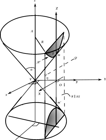
Figura 7.

La situaci n est representada en la Fig:1.7 en la que el plano $\pi$ es $\parallel$ al plano $xz$ y queda definido dando la distancia $VO=\eta$ que suponemos conocida. La $\bigcap$ del cono con el plano $\pi$ es la curva $\mathscr{H}$. Vamos a dm. que $\mathscr{H}$ es una hip rbola y a definir todos sus elementos: focos, directriz, excentricidad, etc.
Definimos ejes $XYZ$ paralelos a $xyz$ y con origen en $O(0,\eta,0),$ Fig:1.7. Las ecuaciones de transf. de coordenadas son:

(133) $$\left\mathchar 46\relax\begin{split}x=X\\ y=Y+\eta\\ z=Z\end{split}\right\}$$

Ahora, la ecuaci n del cono$\diagup xyz$ es: $x^{2}+y^{2}=\tan^{2}\alpha\cdot z^{2}$ y al tener en cuenta [133]

(134) $$X^{2}+{\left(Y+\eta\right)}^{2}=\tan^{2}\alpha\cdot Z^{2}:\text{ecuaci n del cono$\diagup XYZ$ con origen en $0\mathchar 46\relax$}$$

$\pi=\left\{(X,Y,Z)\diagup Y=0\right\}\mathchar 46\relax$ O sea que la ecuaci n del plano $\pi\diagup XYZ$ es $Y=0$ que llevada a [134] nos da:

$$X^{2}+\eta^{2}=\tan^{2}\alpha\cdot Z^{2}:\text{ecuaci n de $\mathscr{H}\diagup XYZ$}$$

As que la curva $\mathscr{H}$ est en el plano $XZ$ y tiene ecuaci n:

$$X^{2}+\eta^{2}=\tan^{2}\alpha\cdot Z^{2}$$

$$\tan^{2}\alpha\cdot Z^{2}-X^{2}=\eta^{2}$$

O sea que

$$\dfrac{Z^{2}}{{\left(\dfrac{\eta}{\tan\alpha}\right)}^{2}}-\dfrac{X^{2}}{\eta^{2}}=1$$

lo que nos dm. que $\mathscr{H}$ es una hip rbola.
Si miramos la curva y sus ejes desde el punto $V$ aparece as :

Figura 8.

$$a=\dfrac{\eta}{\tan\alpha};\quad b=\eta;\quad c=\sqrt{a^{2}+b^{2}}=\sqrt{\dfrac{\eta^{2}}{\tan^{2}\alpha}+\eta^{2}}=\dfrac{\eta}{\tan\alpha}\sqrt{1+\tan^{2}\alpha}=\dfrac{\eta}{\sin\alpha}$$

N tese que

$$\tan\alpha=\dfrac{\sin\alpha}{\cos\alpha}\quad\therefore\quad\sin\alpha=\cos\alpha\cdot\tan\alpha\underset{\overset{\uparrow}{\cos\alpha<1}}{<}\tan\alpha$$

Luego

$$\dfrac{\eta}{\tan\alpha}<\dfrac{\eta}{\sin\alpha},\quad\text{o sea que $a<c\mathchar 46\relax$}$$

$$\epsilon=\dfrac{c}{a}=\dfrac{\dfrac{\eta}{\sin\alpha}}{\dfrac{\eta}{\tan\alpha}}=\sec\alpha\mathchar 46\relax$$

Esto es un hecho sorprendente!.
Todos las secciones obtenidas al cortar el cono con planos $\parallel$s al plano xy son hip rbolas con la misma excentricidad: $\epsilon=\sec\alpha$.
La directriz $\mathscr{DD}$ se localiza as (Fig. 1.8.):

$$\dfrac{a}{\epsilon}=\dfrac{\dfrac{\eta}{\tan\alpha}}{\sec\alpha}=\dfrac{\eta\cos^{2}\alpha}{\sin\alpha}\mathchar 46\relax$$

Las coordenadas del foco $F\diagup XYZ$ son $\left(0,0,c=\dfrac{\eta}{\sin\alpha}\right)$ y respecto a $xyz$ ser an, regresando a [133],

$$x =0$$

$$y =\eta\quad\therefore\quad z=\dfrac{1}{\sin\alpha}y$$

$$z =\dfrac{\eta}{\sin\alpha}$$

Esto nos se ala que cuando el plano $\pi$ se desplaza paralelamente a $xy,$ el foco $F$ de la hip rbola se mueve por la recta

$$\begin{cases}x&=0\\ t&=\dfrac{1}{\sin\alpha}y\end{cases}\mathchar 46\relax$$

Ahora cortemos el cono con un plano $\pi$ no $\parallel$ al eje del cono.
Llamemos $\beta$ al ngulo que hace el plano $\pi$ con el eje del cono y $0$ al punto donde el plano $\pi$ corta al eje del cono, $0\neq V\mathchar 46\relax$

Figura 9.

Vamos a dm. que

• Si $0<\beta<\alpha,$ la secci n es una hip rbola.
  

• Si $\beta=\alpha,$ la secci n es una par bola.
  

• $\beta_{i}\quad\alpha<\beta<\pi/2,$ la secci n c nica es una elipse. (Fig. 1.9)

Recordemos que $x^{2}+y^{2}=\tan^{2}\alpha\cdot z^{2}$ es la ecuaci n del cono$\diagup xyz$ con origen (Fig. 1.10.)
Llamemos $h=0V\mathchar 46\relax$
Primero vamos a trasladar los ejes $XYZ$ con origen en $V$ al punto $O$ donde $O(0,0,h)\diagup xyz\mathchar 46\relax$

Figura 10.

Las ecuaciones de la transformaci n son:

$$x =x^{\prime}$$

$$y =y^{\prime}$$

$$z =z^{\prime}-h$$

que llevamos a la ecuaci n del cono obteniendo: $\tan^{2}\alpha{(z-h)}^{2}=x^{\prime 2}+y^{\prime 2}:$ ecuaci n del cono$\diagup x^{\prime}y^{\prime}z^{\prime}$ con origen en $O\mathchar 46\relax$ Ahora consideremos el sistema ortogonal $XYZ$ con origen en $O$ y conseguido al rotar los ejes $x^{\prime}y^{\prime}z^{\prime}$ un ngulo $\pi/2-\beta\circlearrowleft$ al rededor del eje $x^{\prime}\mathchar 46\relax$
Si $i,j,k,I,J,K$ son los vectores unitarios en las direcciones de los ejes,

$$I =i$$

$$J =\sin\beta j+\cos\beta k$$

$$K =-\cos\beta j+\sin\beta k$$

N tese que la curva $\Sigma,$ intersecci n de $\pi$ con el cono est en el plano $XY$ y que el eje $Z$ es $\perp$ a $\pi\mathchar 46\relax$
Sea $P(x^{\prime},y^{\prime},z^{\prime})$ ( $P(X,Y,Z)$) un punto cualquiera del cono.
Entonces $[\vec{OP}]_{ijk}=[I]_{ijk}^{IJK}[\vec{OP}]_{IJK}\mathchar 46\relax$ O sea que

$$\left(\begin{array}[]{cc}x^{\prime}\\ y^{\prime}\\ z^{\prime}\end{array}\right) =\left(\begin{array}[]{ccc}1&0&0\\ 0&\sin\beta&-\cos\beta\\ 0&\cos\beta&\sin\beta\end{array}\right)\left(\begin{array}[]{cc}X\\ Y\\ Z\end{array}\right)$$

$$\therefore\quad x^{\prime} =X$$

$$y^{\prime} =\sin\beta Y-\cos\beta Z$$

$$z^{\prime} =\cos\beta Y+\sin\beta Z$$

que llevamos a la ecuaci n del cono$\diagup x^{\prime}y^{\prime}z^{\prime}\mathchar 46\relax$

$$\tan^{2}\alpha{\left(\cos\beta Y+\sin\beta Z-h\right)}^{2}=X^{2}+{\left(\sin\beta Y-\cos\beta Z\right)}^{2}:\text{ecuaci n del cono$\diagup XYZ$}$$

Si en la ecuaci n anterior hacemos $Z=0$ obtenemos la ecuaci n de la curva $\Sigma$. O sea que

$$\tan^{2}\alpha{\left(\cos\beta Y-h\right)}^{2}=X^{2}+\sin^{2}\beta Y^{2}$$

es la ecuaci n de $\Sigma\diagup XY$ y que podemos simplificar as :

$$\tan^{2}\alpha\left(\cos^{2}\beta Y^{2}-2h\cos\beta Y+h^{2}\right)=X^{2}+\sin^{2}\beta Y^{2}$$

$$X^{2}+\left(\sin^{2}\beta-\tan^{2}\alpha\cos^{2}\beta\right)Y^{2}+2h\tan^{2}\alpha\cos\beta Y=h^{2}\tan^{2}\alpha\quad\star$$

Vamos a analizar tres casos en la ecuaci n $\star\mathchar 46\relax$

1. Supongamos que $\beta=\alpha\mathchar 46\relax$ Esto significa que $\pi$ es $\parallel$ a una generatriz del cono. El coeficiente de $Y^{2}$ en la ecuaci n $\star$ se anula y la ecuaci n de $\Sigma\diagup XY$ es:

   $$X^{2}+2h\tan^{2}\alpha\cos\alpha Y=\tan^{2}\alpha h^{2}$$

   $$\therefore\quad Y=-\dfrac{1}{2h\tan^{2}\alpha\cos\alpha}X^{2}+\dfrac{h}{2\cos\alpha}$$

   La secci n $\Sigma$ es una PAR BOLA.
   Los elementos de la curva, foco, directriz, etc… se calculan f cilmente$\diagup XY\mathchar 46\relax$

   

   Figura 11.

   
   

   Si $X=0,\quad Y=OV=\dfrac{h}{2\cos\alpha}$
   Si $Y=0,\quad O=-\dfrac{1}{2h\tan^{2}\alpha\cos\alpha}OA^{2}+\dfrac{h}{2\cos\alpha}$

   $$OA^{2} =\dfrac{h}{\cancel{2}\cos\alpha}\cancel{2}h\tan^{2}\alpha\cos\alpha=\dfrac{h^{2}}{\cancel{\cos\alpha}}\tan\alpha\cancel{\cos\alpha}$$

   $$OA^{2} =h\tan\alpha$$

   Como $A$ est en la par bola, $AD=AF\mathchar 46\relax$ O sea que

   $$\dfrac{h}{2\cos\alpha}+\dfrac{p}{2} =\sqrt{h^{2}\tan^{2}\alpha+{\left(\dfrac{h}{2\cos\alpha}-\dfrac{p}{2}\right)}^{2}}$$

   $${\left(\dfrac{h}{2\cos\alpha}+\dfrac{p}{2}\right)}^{2} =h^{2}\tan^{2}\alpha+{\left(\dfrac{h}{2\cos\alpha}+\dfrac{p}{2}\right)}^{2}$$

   $$\therefore\quad p=h\tan^{2}\alpha\cos\alpha=d(F;\mathscr{DD}):\text{distancia foco-directriz}$$

   El foco $F$ se localiza as :

   $$OF=\dfrac{h}{2\cos\alpha}-\dfrac{h\tan^{2}\alpha\cos\alpha}{2}=\dfrac{1}{2\cos\alpha}(1-\sin^{2}\alpha)$$

2. Supongamos ahora que $\alpha<\beta<\pi/2$ y consideremos la c nica $\Sigma$

   $$X^{2}+\left(\sin^{2}\beta-\tan^{2}\alpha\cos^{2}\beta\right)Y^{2}+2h\tan^{2}\alpha\cos\beta Y-h^{2}\tan^{2}\alpha=0$$

   Vamos a emplear lo estudiado en las secciones anteriores para reducirla. Si consideramos la ecuaci n general de las c nicas $AX^{2}+2BY+CY^{2}+2DX+2EY+F$ se tiene que
   $\begin{cases}A=1\\ B=0\\ C=\sin^{2}\beta-\tan^{2}\alpha\cos^{2}\beta\\ D=0\\ 2E=2h\tan^{2}\alpha\cos\beta\quad\therefore\quad E=h\tan^{2}\alpha\cos\beta\\ F=-h^{2}\tan^{2}\alpha\end{cases}$
   Llamemos $e=\dfrac{\cos\beta}{\cos\alpha}\mathchar 46\relax$ Como $\alpha<\beta,\quad\cos\beta<\cos\alpha$ y por lo tanto, $e=\dfrac{\cos\beta}{\cos\alpha}<1\mathchar 46\relax$ Vamos a dm. que en ste $\Sigma$ es una elipse de excentricidad $e=\dfrac{\cos\beta}{\cos\alpha}\mathchar 46\relax$
   Como $e=\dfrac{\cos\beta}{\cos\alpha},\quad\cos\beta=e\cos\alpha\mathchar 46\relax$
   Luego

   $$C =\sin^{2}\beta-\tan^{2}\alpha^{2}\beta=1-\cos^{2}\beta-\tan^{2}\alpha\cos^{2}\beta$$

   $$=1-\cos^{2}\beta(1+\tan^{2}\alpha)=1-\cos^{2}\beta\sec^{2}\alpha\underset{\overset{\uparrow}{\cos\beta}=e\cos\alpha}{=}1-e^{2}\cos^{2}\alpha\sec^{2}\alpha=1-e^{2}$$

   y la ecuaci n de $\Sigma$ puede ponerse as :

   $$X^{2}+(1-e^{2})Y^{2}+2h\tan^{2}\alpha\cos\beta Y-h^{2}\tan^{2}\alpha=0\quad\text{con}1-e^{2}>0$$

   $$M=\left(\begin{array}[]{cc}A&B\\ B&C\end{array}\right)=\left(\begin{array}[]{cc}1&0\\ 0&1-e^{2}\end{array}\right);\quad\delta=|M|=1-e^{2} =C$$

   Para hallar el centro debe resolverse el sistema:$\begin{cases}Ax+By=-D\\ Bx+Cy=-E\end{cases}$
   O sea
   $\begin{cases}1\cdot x+0\cdot y=0\\ 0\cdot x+(1-e^{2})y=-h\tan^{2}\alpha\cos\beta\end{cases}$
   Hay soluci n nica:

   $$\widetilde{h}=0,\quad\widetilde{k}=-\dfrac{h\tan^{2}\alpha\cos\beta}{1-e^{2}} \underset{\uparrow}{<}0$$

   $$1-e^{2}>0$$

   $$\begin{array}[]{cc}\text{y por lo tanto se trata de}\\ \text{una c nica con centro nico}\end{array}$$

   

   Figura 12.

   
   

   Al trasladar los ejes $XY$ al punto $O^{\prime}$ de coor. $\left(0,-\dfrac{h\tan^{2}\alpha\cos\beta}{1-e^{2}}\right)\diagup X$ se eliminan los t rminos lineales en $\star\mathchar 46\relax$
   La ecuaci n de la c nica $\Sigma\diagup\overline{X}\overline{Y}$ con origen en $O^{\prime}$ es:

   $$\overline{X}^{2}+(1-e^{2})\overline{Y}^{2}=-\dfrac{\Delta}{\delta}$$

   $$\dfrac{\Delta}{\delta} =\dfrac{1}{1-e^{2}}\left|\begin{array}[]{ccc}A&B&D\\ B&C&E\\ D&E&F\end{array}\right|=\dfrac{1}{1-e^{2}}\left|\begin{array}[]{ccc}1&0&0\\ 0&1-e^{2}&h\tan^{2}\alpha\cos\beta\\ 0&h\tan^{2}\alpha\cos\beta&-h^{2}\tan^{2}\alpha\end{array}\right|$$

   $$=\dfrac{1}{1-e^{2}}\left[-(1-e^{2})h^{2}\tan^{2}\alpha-h^{2}\tan^{4}\cos^{2}\beta\right]$$

   $$\underset{\uparrow}{=}\left[-(1-e^{2})h^{2}\tan^{2}\alpha-h^{2}e^{2}\tan^{2}\alpha(1-\cos^{2}\alpha)\right]$$

   $$\begin{cases}\tan^{4}\alpha\cos^{2}\beta\underset{\overset{\uparrow}{\cos\beta}=e\cos\alpha}{=}\tan^{4}\alpha{(e\cos\alpha)}^{2}&=e^{2}\tan^{2}\alpha\dfrac{\sin^{2}\alpha}{\cancel{\cos^{2}\alpha}}\cancel{\cos^{2}\alpha}\\ &=e^{2}\tan^{2}\alpha\sin^{2}\alpha\\ &=e^{2}\tan^{2}\alpha(1-\cos^{2}\alpha)\end{cases}$$

   $$=\dfrac{1}{1-e^{2}}\left[h^{2}e^{2}\tan^{2}\alpha\cos^{2}\alpha\cdot h^{2}\tan^{2}\alpha\right]$$

   $$=\dfrac{h^{2}\tan^{2}\alpha}{1-e^{2}}(e^{2}\cos^{2}\alpha-1)=\dfrac{h^{2}\tan^{2}\alpha}{1-e^{2}}(\cos^{2}\beta-1)$$

   Luego

   $$-\dfrac{\Delta}{\delta}=\dfrac{h^{2}\tan^{2}\alpha}{1-e^{2}}(1-\cos^{2}\beta)=\dfrac{h^{2}\tan^{2}\alpha\cdot\sin^{2}\beta}{1-e^{2}}$$

   La ecuaci n de la c nica $\Sigma\diagup\overline{X}\overline{Y}$ es finalmente

   $$\overline{X}^{2}+(1-e^{2})\overline{Y}^{2}=\dfrac{h^{2}\tan^{2}\alpha\sin^{2}\beta}{1-e^{2}}$$

   que podemos finalmente escribir as :

   $$\dfrac{\overline{X}^{2}}{{\left(\dfrac{h\tan\alpha\sin\beta}{\sqrt{1-e^{2}}}\right)}^{2}}+\dfrac{\overline{Y}^{2}}{{\left(\dfrac{h\tan\alpha\sin\beta}{1-e^{2}}\right)}^{2}}=1$$

   lo que nos dm. que la curva $\Sigma$ es una Elipse de centro en $O^{\prime}$.

   

   Figura 13.

   
   

   en la que los semiejes son

   $$O^{\prime}A =a=\dfrac{h\tan\alpha\sin\beta}{\sqrt{1-e^{2}}}$$

   y

   $$O^{\prime}V =b=\dfrac{h\tan\alpha\sin\beta}{1-e^{2}};\quad e=\dfrac{\cos\beta}{\cos\alpha}<1$$

   Vamos a dm. que $a<b$ con lo cual queda establecido que los focos de la elipse est n en el eje $\overline{Y}$ y localizados as :

   $$0^{\prime}F=c=\sqrt{b^{2}-a^{2}}$$

   Sabemos que si $x<1,\quad x^{2}<x\mathchar 46\relax$
   Como $\sqrt{1-e^{2}}<1,\quad 1-e^{2}<\sqrt{1-e^{2}}\mathchar 46\relax$ Luego $\dfrac{1}{\sqrt{1-e^{2}}}<\dfrac{1}{1-e^{2}}$ y por tanto, $\dfrac{h\tan\alpha\sin\beta}{\sqrt{1-e^{2}}}<\dfrac{h\tan\alpha\sin\beta}{1-e^{2}},$ o sea que $a<b\mathchar 46\relax$
   

   $$O^{\prime}F=c=\sqrt{b^{2}-a^{2}}=h\tan\alpha\sin\beta\dfrac{1}{1-e^{2}}\mathchar 46\relax$$

   Sea $\epsilon$ la excentricidad de $\Sigma\mathchar 46\relax$
   

   $$c=0F^{\prime}=\epsilon b\quad\therefore\quad\epsilon=\dfrac{c}{b}=\dfrac{h\tan\alpha\sin\beta\frac{e}{1-e^{2}}}{\dfrac{h\tan\alpha\sin\beta}{1-e^{2}}}=e=\dfrac{\cos\beta}{\cos\alpha}$$

   Esto dm. que la excentricidad $\epsilon$ de la elipse es la misma para todas las elipses obtenidas al cortar el cono con los planos $\parallel$s a $\pi\mathchar 46\relax$
   

3. Supongamos que $0<\beta<\alpha$ y consideremos la c nica

   $$\Sigma:X^{2}+\left(\sin^{2}\beta-\tan^{2}\alpha\cos^{2}\beta\right)Y^{2}+2h\tan^{2}\alpha\cos\beta Y-h^{2}\tan^{2}\alpha=0$$

   De nuevo:

   $$A =1$$

   $$B =0$$

   $$C =\sin^{2}\beta-\tan^{2}\alpha\cos^{2}\beta$$

   $$D =0$$

   $$E =h\tan^{2}\alpha\cos\beta$$

   $$F =-h\tan^{2}\alpha$$

   Llamemos $e=\dfrac{\cos\beta}{\cos\alpha}\mathchar 46\relax$ Como $\beta<\alpha,\quad\cos\beta>\cos\alpha$ y se tiene ahora que $e=\dfrac{\cos\beta}{\cos\alpha}>1\quad\therefore e^{2}-1\quad\text{y}1-e^{2}<0\mathchar 46\relax$
   Vamos a dm. que $\Sigma$ es una hip rbola de excentricidad $e$.
   En este caso,

   $$C =\sin^{2}\beta-\tan^{2}\alpha\cos^{2}\beta=1-\cos^{2}\beta-\tan^{2}\alpha\cos^{2}\beta$$

   $$=1-\cos^{2}\beta(1-\tan^{2}\alpha)=1-\cos^{2}\beta\sec^{2}\alpha$$

   $$\underset{\nearrow}{=}1-e^{2}\cos^{2}\alpha\sec^{2}\alpha=1-e^{2}<0$$

   $$\cos\beta=e\cos\alpha$$

   y la ecuaci n de la c nica se puede escribir:

   $$X^{2}+(1-e^{2})Y^{2}+2h\tan^{2}\alpha\cos\beta Y-h^{2}\tan^{2}\alpha=0$$

   con $1-e^{2}<0\mathchar 46\relax$
   En an lisis de centros es el mismos que hizo en el caso [2)].
   La c nica tiene centro nico en $O^{\prime}\left(0,-\dfrac{h\tan^{2}\alpha\cos\beta}{1-e^{2}}\right),$ solo que ahora $1-e^{2}<0\mathchar 46\relax$ O sea que el centro $O^{\prime}$ est situado as :

   

   Figura 14.

   
   

   Al trasladar los ejes al centro $O^{\prime}$ de la c nica, desaparecen los t rminos lineales y la ecuaci n de $\Sigma\diagup\overline{X},\overline{Y}$ es:

   $$\overline{X}^{2}+(1-e^{2})\overline{Y}^{2}=-\dfrac{\Delta}{\delta}\quad\text{con}\quad 1-e^{2}<0\mathchar 46\relax$$

   El c lculo de $-\dfrac{\Delta}{\delta}$ es el mismo que se llev a cabo en el caso [2)]:

   $$-\dfrac{\Delta}{\delta}=\dfrac{h^{2}\tan^{2}\alpha\sin^{2}\beta}{1-e^{2}}\quad\text{con}\quad 1-e^{2}<0\mathchar 46\relax$$

   La ecuaci n de la c nica$\diagup\overline{X}\overline{Y}$ es

   $$\overline{X}^{2}+(1-e^{2})\overline{Y}^{2} =\dfrac{h^{2}\tan^{2}\alpha\sin^{2}\beta}{1-e^{2}}\quad\text{y con}\quad 1-e^{2}<0,$$

   $$\overline{X}^{2}-(1-e^{2})\overline{Y}^{2} =-\dfrac{h^{2}\tan^{2}\alpha\sin^{2}\beta}{e^{2}-1}\quad\text{con}\quad e^{2}-1<0$$

   O sea que la ecuaci n es:

   $$\dfrac{\overline{Y}^{2}}{{\left(\dfrac{h\tan\alpha\sin\beta}{e^{2}-1}\right)}^{2}}-\dfrac{\overline{X}^{2}}{{\left(\dfrac{h\tan\alpha\sin\beta}{\sqrt{e^{2}-1}}\right)}^{2}}=1$$

   lo que nos indica que $\Sigma$ es una Hip rbola de centro en $O^{\prime}\mathchar 46\relax$
   y con semiejes

   $$O^{\prime}V^{\prime} =b=\dfrac{h\tan\alpha\sin\beta}{e^{2}-1}$$

   $$V^{\prime}N =a=\dfrac{h\tan\alpha\sin\beta}{\sqrt{e^{2}-1}}\quad[Fig\mathchar 46\relax]$$

   $$O^{\prime}N =c=\sqrt{a^{2}+b^{2}}=\sqrt{\dfrac{h^{2}\tan^{2}\alpha\sin^{2}\beta}{e^{2}-1}+\dfrac{h^{2}\tan^{2}\alpha\sin^{2}\beta}{{(e^{2}-1)}^{2}}}=$$

   $$=h\tan\alpha\sin\beta\dfrac{e}{e^{2}-1}$$

   

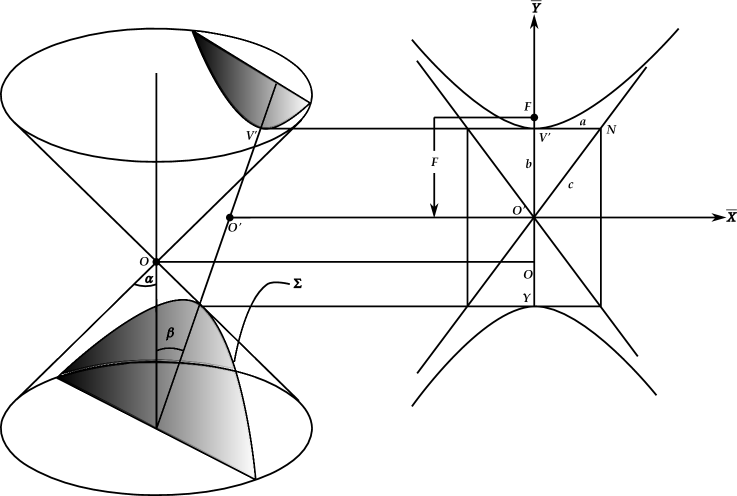
   Figura 15.

   
   

   Llamemos $\epsilon$ a la excentricidad de $\Sigma$ y $F$ al foco.
   

   $$c=0^{\prime}F=\epsilon p\quad\therefore\quad\epsilon=\dfrac{c}{b}=\dfrac{h\tan\alpha\sin\beta\dfrac{e}{e^{2}-1}}{\dfrac{h\tan\alpha\sin\beta}{e^{2}-1}}=e=\dfrac{\cos\beta}{\cos\alpha}$$

   lo que nos dm. que todas las hip rbolas obtenidas al cortar el cono con los planos $\parallel$s a $\pi$ tienen la misma excentricidad:

   $$\epsilon=\dfrac{\cos\beta}{\cos\alpha}>1$$

12. Intersecci n de un cilindro circular recto con un plano que corta al eje del cilindro

Consideremos el cilindro circular recto de radio $R$ y cuyo eje es el eje $z$. Su ecuaci n es
$\begin{cases}x^{2}+y^{2}=R^{2}\\ z\in\mathbb{R}\end{cases}$
Si lo cortamos con un plano $\pi$ que pase por $O$ y haga con el eje $z$ un ngulo $\beta$, la curva que se obtiene es una elipse de excentricidad $\epsilon=\cos\beta\mathchar 46\relax$ Vamos a demostrar esto.

Figura 16.

Si giramos los ejes $xyz$ un ngulo $\pi/2-\beta\circlearrowleft$ al rededor del eje $x$ obtenemos un sistema $XYZ$ en el que eje $Z$ es $\perp$ al plano $\pi$ y los ejes $X$ y $Y$ est n en $\pi\mathchar 46\relax$
Sea $P$ un punto del cilindro de coord. $(x,y,z)$ y $(X,Y,Z)$ respecto a los ejes $xyz$ y $XYZ\mathchar 46\relax$

$$[\vec{OP}]_{ijk}=\left(\begin{array}[]{cc}x\\ y\\ z\end{array}\right) =[I]_{ijk}^{IJK}[\vec{OP}]_{IJK}$$

O sea que

$$\left(\begin{array}[]{cc}x\\ y\\ z\end{array}\right) =\left(\begin{array}[]{ccc}1&0&\\ 0&\sin\beta&-\cos\beta\\ 0&\cos\beta&\sin\beta\end{array}\right)\left(\begin{array}[]{cc}X\\ Y\\ Z\end{array}\right)$$

$$\therefore\quad x =X$$

$$y =\sin\beta Y-\cos\beta Z$$

$$z =\cos\beta Y+\sin\beta Z$$

As que la ecuaci n del cilindro$\diagup XYZ$ es:

$$X^{2}+{\left(\sin\beta Y-\cos\beta Z\right)}^{2}=R^{2}$$

$$X^{2}+\sin^{2}\beta Y^{2}-2\cos\beta\sin\beta YZ+\cos^{2}\beta Z^{2}=R^{2}$$

Si $Z=0,$ obtenemos la ecuaci n de la secci n del cilindro con el plano:

$$X^{2}+\sin^{2}Y^{2} =R^{2}$$

$$\dfrac{X^{2}}{R^{2}}+\dfrac{Y^{2}}{{\left(\dfrac{R}{\sin\beta}\right)}^{2}} =1\quad\text{Elipse}$$

$$a =R$$

$$b =\dfrac{R}{\sin\beta}>R=a,$$

lo cual explica que los focos est n en el eje $Y\mathchar 46\relax$

$$c=OF=\sqrt{{\left(\dfrac{R}{\sin\beta}\right)}^{2}-R^{2}}=\dfrac{R\cos\beta}{\sin\beta}=\dfrac{R}{\tan\beta}$$

Si $\epsilon$ es la excentricidad de la curva,

$$\epsilon=\dfrac{c}{b}=\dfrac{R\dfrac{\cos\beta}{\sin\beta}}{\dfrac{R}{\sin\beta}}=\cos\beta$$