How to Schedule the Marketing of Products with
Negative Externalities

Abstract

In marketing products with negative externalities, a schedule which specifies an order of consumer purchase decisions is crucial, since in the social network of consumers, the decision of each consumer is negatively affected by the choices of her neighbors. In this paper, we study the problems of finding a marketing schedule for two asymmetric products with negative externalites. The goals are two-fold: maximizing the sale of one product and ensuring regret-free purchase decisions. We show that the maximization is NP-hard, and provide efficient algorithms with satisfactory performance guarantees. Two of these algorithms give regret-proof schedules, i.e. they reach Nash equilibria where no consumers regret their previous decisions. Our work is the first attempt to address these marketing problems from an algorithmic point of view.

Keywords: Negative externality, Social network, Nash equilibrium, Efficient algorithm, Marketing schedule

1 Introduction

The total value of any (consumer) product can be roughly classified into three parts: physical value, emotional value, and social value [11]. With the fast development of economy, the basic physical needs of more and more consumers are easily met. Consequently, people increasingly shift their attention to emotional and social values when they consider whether to buy a product. In particular, the social value, whose amount is not determined by what a consumer consumes alone or how she personally enjoys it, but by the comparisons with what other people around her consume, is becoming a more and more crucial ingredient for both consumer purchase and therefore seller marketing. For many products, whether they will be welcome depends mainly on how much social value they can provide to the consumers. This is especially true for fashionable and luxury goods, where the products often exhibit negative (consumption) externalities – they become less valuable as more people use them [1, 9].

The comparison that a consumer makes, for calculating the social value of a product, is naturally restricted to her neighbors in the social network. For a consumer, the social value of a product with negative externality is often proportional to the number of her neighbors who do not consume this product [9]. In the market, the purchase decisions of a consumer often depend on the values of the products at the time they are promoted – the product of larger value will be selected. In contrast to the physical and emotional values, which are relatively fixed, the social values of products vary with different marketing schedules. The goal of this paper is to design good marketing schedules for promoting products with negative externalities in social networks.

Motivation and related work Our study is motivated by the practical marketing problem concerning how to bring the products to consumers’ attention over time. Among a large literature on diffusion of competing products or opinions in social networks (see e.g., [2, 7, 8] and references therein), Chierichetti, Kleinberg and Pancones [7] recently studied the scheduling aspect of the diffusion problem on two products – finding an order of consumer purchase decision making to maximize the adoption of one product. In their model, the two competing products both have positive (consumption) externalities and every consumer follows the majority of her social network neighbors when the externalities outweigh her own internal preference. The authors [7] provided an algorithm that ensures an expected linear number of favorable decisions.

The network-related consumption externalities have been classified into four categories [6]. Comparing to the other three, the negative cross-consumer externality, as considered in this paper, has been far less studied [1, 9], and was emphasized for its importance in management and marketing nowdays [6].

The model studied in this paper can also be taken as an extension of one side of the fashion game, which was formulated by Jackson [10]. Very interestingly, people often have quite different, in fact almost opposite, opinions on what is fashionable, e.g., “Lady Gaga is Godness of fashion” vs “This year’s fashion color is black”. Following Jackson, we call consumers holding the former “personality reflection” idea of fashion rebels and the latter “prevailing style” idea conformists. More generally, a consumer behaves like a rebel (conformist) if the product, from her point of view, has negative (positive) externality. In an era emphasizing personal identities, more and more consumers would like to be rebels. For example, they would prefer Asian-style pants, when seeing many friends and colleagues (their social network neighbors) wearing European-style. However, the rebel social network is still under-researched in comparison with vast literature on conformist social networks. For a market where all the consumers are rebels, as considered in this paper, it has been previously studied by several papers under the term of anti-coordination [4, 5].

Model formulation The market is represented by a social network $G=(V,E)$, an undirected graph with node set $V$ consisting of $n$ consumers and link set $E$ of $m$ connections between consumers. A seller has two (types of) products $\mathcal{Y}$ and $\mathcal{N}$ with similar functions. We abuse notations by using $\mathcal{Y}$ and $\mathcal{N}$ to denote both types and products.

The marketing is done sequentially: The seller is able to ask the consumers one by one whether they are more interested in $\mathcal{Y}$ or in $\mathcal{N}$. Each consumer buys (chooses) exactly one of $\mathcal{Y}$ and $\mathcal{N}$, whichever provides her a larger total value, only at the time she is asked. This is a simplification of the so called precision marketing [13]. For every consumer, a product of type $\mathcal{T}\in\{\mathcal{Y},\mathcal{N}\}$ provides her with total value $p_{{}_{\mathcal{T}}}+s_{{}_{\mathcal{T}}}(x_{{}_{\mathcal{T}}})$, where $p_{{}_{\mathcal{T}}}$ is the sum of physical and emotional values, and $s_{{}_{\mathcal{T}}}(x_{{}_{\mathcal{T}}})$ is the social value determined by decreasing function $s_{{}_{\mathcal{T}}}(\cdot)$ and the number $x_{{}_{\mathcal{T}}}$ of her neighbors who have bought product $\mathcal{T}$. We assume that $\mathcal{Y}$ is very similar to $\mathcal{N}$ with $p_{{}_{\mathcal{Y}}}>p_{{}_{\mathcal{N}}}$ and the externality outweighs the physical and emotional difference, i.e., for any permutation $\mathcal{T},\mathcal{F}$ of $\mathcal{Y},\mathcal{N}$ and any nonnegative integers $x,y$ ($x<y$) we have $s_{{}_{\mathcal{T}}}(x)-s_{{}_{\mathcal{F}}}(x)<p_{{}_{\mathcal{Y}}}-p_{{}_{\mathcal{N}}}<s_{{}_{\mathcal{T}}}(x)-s_{{}_{\mathcal{F}}}(y)$.

Actually, the above model can be summarized as the following scheduling problems on rebel social networks.

Rebels. Every consumer is a rebel who, at her turn to choose from $\{\mathcal{Y},\mathcal{N}\}$, will buy the product different from the one currently possessed by the majority of her neighbors. If there are equal numbers of neighbors having bought $\mathcal{Y}$ and $\mathcal{N}$ respectively, the consumer will always buy $\mathcal{Y}$.

Scheduling. A (marketing) schedule $\pi$, for network $G$ is an ordering of consumers in $V$ which specifies the order $\pi(v)\in\{1,2,\ldots,n\}$ of consumer $v\in V$ being asked to buy (choose) $\mathcal{Y}$ or $\mathcal{N}$, or “being scheduled” for short. We refer to the problem of finding a schedule for a rebel social network as the rebel scheduling problem. Given schedule $\pi$, the choice (purchase decision) of each consumer $v$ under $\pi$ is uniquely determined, and we denote it by $\pi[v]$, which belongs to $\{\mathcal{Y},\mathcal{N}\}$. The decisions of all consumers form the marketing outcome $(\pi[v]:v\in V)$ of $\pi$. The basic goal of the rebel scheduling problem is to find a schedule whose outcome contains $\mathcal{Y}$ (resp. $\mathcal{N}$) decisions as many as possible because $\mathcal{Y}$ (resp. $\mathcal{N}$) is more profitable for the seller.

Equilibrium. As seen above, the value of a product changes as the marketing proceeds. Every schedule corresponds to a dynamic game among consumers. We assume that consumers behave naively without predictions. A natural question is: Can these simple behaviors (or equivalently, a schedule) eventually lead to a Nash equilibrium – a state where no consumer regrets her previous decision? This question is of both theoretical and practical interests. Schedules that lead to Nash equilibria are called regret-proof; they guarantee high consumer satisfaction, which is beneficial to the seller’s future marketing.

Results and contribution We prove that it is NP-hard to find a marketing schedule that maximizes the number of $\mathcal{Y}$ (resp. $\mathcal{N}$) decisions. Complementary to the NP-hardness, we design $O(n^{2})$-time algorithms for finding schedules that guarantee at least $n/2$ decisions of $\mathcal{Y}$, and at least $n/3$ decisions of $\mathcal{N}$, respectively. The numbers $n/2$ and $n/3$ are best possible for any algorithm. Let $\alpha$ denote the size of maximum independent set of $G$. We show that regret-proof schedules that guarantee at least $n/2$ decisions of $\mathcal{Y}$ and at least $\max\{\sqrt{n+1}-1,(n-\alpha)/2\}$ decisions of $\mathcal{N}$, respectively, can be found in time $O(mn^{2})$. In contrast, decentralized consumer choices without a schedule might result in an arbitrarily worse outcome. This can be seen from the star network, where in the worst case only one consumer chooses the product consistent with the seller’s objective.

To the best of our knowledge, this paper is the first attempt to address the scheduling problems for marketing products with negative externalities (i.e marketing in rebel social networks). Our algorithms for maximizing the number of $\mathcal{Y}$ decisions can be extended to deal with the case of promoting one product where $\mathcal{Y}$ and $\mathcal{N}$ are interpreted as buying and not buying, respectively.

2 Maximization

We study the rebel scheduling problem to maximize seller’s profits in Subsections 2.1 and 2.2, respectively, for the cases of $\mathcal{Y}$ and $\mathcal{N}$ having higher net profits.

Throughout we consider $G=(V,E)$ a connected rebel social network for which we have $n=O(m)$. All results can be extended to any network without isolated nodes. Let $\pi$ be a schedule for $G$, and $u,v\in V$. We say that $\pi$ schedules $v\in V$ with decision $\pi[v]\in\{\mathcal{Y},\mathcal{N}\}$, and $\pi$ schedules $u$ before $v$ if $\pi(u)<\pi(v)$.

2.1 When $\mathcal{Y}$ is more profitable

It is desirable to find an optimal schedule that maximizes the number of consumers purchasing $\mathcal{Y}$. Although this turns out to be a very hard task (Theorem 2.1), we can guarantee that at least half of the consumers choose $\mathcal{Y}$ (Theorem 2.2).

Theorem 2.1.

The rebel scheduling problem for maximizing the number of $\mathcal{Y}$ decisions is NP-hard.

Proof.

We prove by reduction from the maximum independent set problem. Given any instance of the maximum independent set problem on connected graph $H=(N,F)$, by adding some pendant nodes to $H$ we construct in polynomial time a network $G$ (an instance of the rebel scheduling problem): For each node $u\in N$ with degree $d(u)$ in $H$, we add a set $P_{u}$ of $d(u)$ nodes, and connect each of them to $u$. The resulting network $G=(V,E)$ is specified by $V:=N\cup(\cup_{u\in N}P_{u})$ and $E:=F\cup(\cup_{u\in N}\{up:p\in P_{u}\})$, where each node in $V\setminus N=\cup_{u\in N}P_{u}$ is pendant, and each node $u\in N$ is non-pendant and has exactly $2d(u)$ neighbors: half of them are non-pendant nodes in $N$ and the other half are the $d(u)$ pendant nodes in $P_{u}$.

We associate every schedule ${\pi}$ for $G$ with an integer $\theta({\pi})$, equal to the number of pendant nodes which are scheduled (by ${\pi}$) after their unique neighbors. Clearly

$$\theta(\pi)\leq|V\setminus N|=2|F|\text{ for any schedule }\pi\text{ of }G.$$ (2.1)

Claim 1.

For any $u\in N$ and any schedule $\pi$ of $G$, if $\pi$ schedules all nodes in $P_{u}\cup\{u\}$ with $\mathcal{Y}$, then (all the $d(u)$ pendant neighbors of $u$ in $P_{u}$ have to be scheduled before $u$ with decisions $\mathcal{Y}$, therefore) all the $d(u)$ non-pendant neighbors of $u$ have to be scheduled with $\mathcal{N}$ before $u$ is scheduled.

Consider $\pi$ being an optimal schedule for $G$. If $\theta(\pi)=0$, then $\pi$ schedules all pendant nodes before their neighbors, and hence all of these pendant nodes choose $\mathcal{Y}$. It follows from Claim 1 that $\{v\in N:\pi[v]=\mathcal{Y}\}$ is an independent set of $H$. Since $\pi$ is optimal, the independence set is maximum in $H$. Thus, in view of (2.1), to prove the theorem, it suffices to show the following.

Claim 2.

Given an optimal schedule $\pi$ for $G$ with $\theta(\pi)>0$, another optimal schedule $\pi^{\prime}$ for $G$ with $\theta(\pi^{\prime})<\theta(\pi)$ can be found in polynomial time.

Since $\theta(\pi)>0$, we can take $w\in N$ to be the last non-pendant node scheduled by $\pi$ earlier than some of its pendant neighbors. Under $\pi$, let $P_{w}^{\prime}$ ($\emptyset\neq P_{w}^{\prime}\subseteq P_{w}$) be the set of all pendant neighbors of $w$ that are scheduled after $w$, let $U$ be the set of non-pendant nodes scheduled after $w$, and let $P_{U}$ be the set of the pendant nodes whose (non-pendant) neighbors belong to $U$ (possibly $U=\emptyset=P_{U}$). The choice of $w$ implies that $\pi$ schedules every node in $P_{U}$ before its neighbor. Without loss of generality we may assume that under $\pi$,

• (Pendant) nodes in $P_{U}$ are scheduled before all other nodes (with $\mathcal{Y}$).

• (Pendant) nodes in $P_{w}^{\prime}$ are scheduled immediately after $w$ one by one.

• (Non-pendant) nodes in $U$ are scheduled at last.

If $\pi$ schedules $w$ with $\mathcal{N}$, then at later time it schedules all pendant nodes in $P^{\prime}_{w}$ with $\mathcal{Y}$. Another optimal schedule $\pi^{\prime}$ (for $G$) with the same outcome as $\pi$ can be constructed as follows: $\pi^{\prime}$ schedules nodes in $P^{\prime}_{w}$ first, and then schedules other nodes of $V$ in a relative order the same as $\pi$. Clearly, $\pi^{\prime}$ with $\theta(\pi^{\prime})\leq\theta(\pi)-1$ is the desired schedule. It remains to consider the case where $\pi$ schedules $w$ with

$$\pi[w]=\mathcal{Y}.$$ (2.2)

It follows that $\pi[p]=\mathcal{N}$ for all $p\in P_{w}^{\prime}$. Let $\pi^{\prime}$ be the schedule that first schedules nodes of $V\setminus\{w\}$ in a relative order the same as $\pi$, and schedules $w$ finally. It is clear that $\theta(\pi^{\prime})\leq\theta(\pi)-1$ and $\pi^{\prime}[p]=\mathcal{Y}$ for all $p\in P_{w}^{\prime}$. We only need to show that $\pi^{\prime}$ is optimal.

Observe that $\pi^{\prime}$ first schedules every $v\in V$ satisfying $\pi(v)<\pi(w)$ with the same decision as in $\pi$ (particularly, all nodes in $P_{U}$ are scheduled with $\mathcal{Y}$). Subsequently, $\pi^{\prime}$ schedules nodes in $P_{w}^{\prime}$ and $U$ in the same relative order as $\pi$ Finally $\pi^{\prime}$ schedules $w$. Since all pendant nodes in $P^{\prime}_{w}$ ($\neq\emptyset$) are scheduled by $\pi^{\prime}$ with $\mathcal{Y}$, and by $\pi$ with $\mathcal{N}$ the optimality of $\pi^{\prime}$ would follow if $\pi^{\prime}$ schedules every node of $U$ with the same decision as $\pi$.

Suppose it were not the case. Let $u\in U\subseteq N$ be the earliest node in $U$ scheduled by $\pi^{\prime}$ with a decision $\pi^{\prime}[u]$ different from $\pi[u]$. It must be the case that $w$ is a non-pendant neighbor of $u$ and $\pi[w]\neq\pi[u]$. At the time $\pi^{\prime}$ schedules $u$, all pendant neighbors of $u$ in $P_{u}\subseteq P_{U}$ have been scheduled with $\mathcal{Y}$ and the non-pendant neighbor $w$ has not been scheduled, it follows from Claim 1 that $\pi^{\prime}[u]=\mathcal{N}$. As $\pi[u]\neq\pi^{\prime}[u]$ and $\pi[w]\neq\pi[u]$, we have $\pi[w]=\pi^{\prime}[u]=\mathcal{N}$, a contradiction to (2.2). The optimality of $\pi^{\prime}$ is established, which proves Claim 2 and therefore Theorem 2.1. ∎

We next design an algorithm for finding a schedule that ensures at least $n/2$ decisions of $\mathcal{Y}$. The algorithm iteratively constructs a node set $A$ for which there exist two schedules $\pi^{\prime}$ and $\pi^{\prime\prime}$ scheduling each node in $A$ with different decisions. In the end, at least half nodes of $A$ can be scheduled by either $\pi^{\prime}$ or $\pi^{\prime\prime}$ with $\mathcal{Y}$ decisions. Subsequently, the nodes outside $A$, which form an independent set, will all choose $\mathcal{Y}$ (in an arbitrary order).

Algorithm 1.

Input: Network $G=(V,E)$. Output: Partial schedule $\pi$ for $G$.

 

1. Initial setting: $A\leftarrow\emptyset,t\leftarrow 1$, $\pi^{\prime}\leftarrow$ a null schedule

2. While $\exists$ $w\in V\setminus A$ which has different numbers of neighbors in $A$ choosing $\mathcal{Y}$ and $\mathcal{N}$ respectively under $\pi^{\prime}$ do

3. schedule $w$: $\pi^{\prime}(w)\leftarrow t$, $\pi^{\prime\prime}(w)\leftarrow t$;

   $A\leftarrow A\cup\{w\}$, $t\leftarrow t+1$

4. End-while

5. If $\exists$ $uv\in E$ with $u,v\notin A$

   then schedule $uv$: $\pi^{\prime}(u)\leftarrow t,\pi^{\prime}(v)\leftarrow t+1,\pi^{\prime\prime}(v)\leftarrow t,\pi^{\prime\prime}(u)\leftarrow t+1$;

   $A\leftarrow A\cup\{u,v\}$, $t\leftarrow t+2$;

   Go back to Step 2.

6. Let $\pi$ be $\pi^{\prime}$ or $\pi^{\prime\prime}$ whichever schedules more nodes with $\mathcal{Y}$ (break tie arbitrarily)

    

For convenience, we reserve symbol “schedule” for the scheduling (constructing $\pi$ and $\pi^{\prime\prime}$) as conducted at Steps 3 and 5 in Algorithm 1. Similarly, we also say “schedule a node” and “schedule an edge” with the implicit understanding that the node and the edge satisfy the conditions in Step 2 and Step 5 of Algorithm 1.

Claim 3.

$\pi^{\prime}[v]=\mathcal{Y}$ if and only if $\pi^{\prime\prime}[v]=\mathcal{N}$ for all $v\in A$.

Proof.

The algorithm enlarges $A$ gradually at Steps 3 and 5, producing a sequence of node sets $A_{0}=\emptyset$, $A_{1}$, …, $A_{\ell}=A$. We prove by induction on $k$ that $\pi^{\prime}(v)=\mathcal{Y}$ if and only if $\pi^{\prime\prime}(v)=\mathcal{N}$ for all $v\in A_{k}$, $k=0,1,\ldots,\ell$. The base case of $k=0$ is trivial.

Suppose that $k\geq 1$ and the statement is true for $A_{k-1}$. In case of $A_{k}$ being produced at Step 2, suppose $w$ has $n_{1}$ (resp. $n_{2}$) neighbors in $A_{k-1}$ choosing $\mathcal{Y}$ (resp. $\mathcal{N}$) under $\pi^{\prime}$. By hypothesis, $w$ has $n_{1}$ (resp. $n_{2}$) neighbors in $A_{k-1}$ choosing $\mathcal{N}$ (resp. $\mathcal{Y}$) under $\pi^{\prime\prime}$. Since $n_{1}\neq n_{2}$, we see that $\pi^{\prime}[w]=\mathcal{Y}$ if and only if $\pi^{\prime\prime}[w]=\mathcal{N}$. In case of $A_{k}$ being produced at Step 5, both $u$ and $v$ have equal number of neighbors in $A_{k-1}$ choosing $\mathcal{Y}$ and $\mathcal{N}$, respectively, under $\pi^{\prime}$, due to the implementation of the while-loop at Steps 2–4. By hypothesis both $u$ and $v$ have equal number of neighbors in $A_{k-1}$ choosing $\mathcal{Y}$ and $\mathcal{N}$, respectively, under $\pi^{\prime\prime}$. It follows from $uv\in E$ that $\pi^{\prime}[u]=\pi^{\prime\prime}[v]=\mathcal{Y}$ and $\pi^{\prime}[v]=\pi^{\prime\prime}[u]=\mathcal{N}$. In either case, the statement is true for $A_{k}$, proving the claim. ∎

Claim 4.

• At least half nodes of $A$ are scheduled by $\pi$ with $\mathcal{Y}$ (by Step 6).

• The nodes in $V\setminus A$ (if any) form an independent set of $G$ (by Step 5).

• Each node in $V\setminus A$ has an equal number of neighbors in $A$ choosing $Y$ and $\mathcal{N}$, respectively, under $\pi^{\prime}$ (by Steps 2–4), and under $\pi^{\prime\prime}$ (by Claim 3), and hence under $\pi$ (by Step 6).∎

Theorem 2.2.

A schedule that ensures at least $n/2$ decisions of $\mathcal{Y}$ can be found in $O(n^{2})$ time.

Proof.

It follows from Claim 4(ii) and (iii) that $\pi$ can be extended to a schedule for $G$ such that all node in $V\setminus A$ choose $\mathcal{Y}$. By Claim 4(i), the outcome contains at least $n/2$ decisions of $\mathcal{Y}$.

Next we show the time complexity. Algorithm 1 keeps an $n\times 2$ array $[\delta_{v},\delta_{v}^{\prime}]$, $v\in V$, where $\delta_{v}$ represents the difference between the numbers of neighbors of node $v$ in $A$ choosing $\mathcal{Y}$ and $\mathcal{N}$, and $\delta_{v}^{\prime}$ represents the number of neighbors of node $v$ in $V\setminus A$. The initial setting of the array $[\delta_{v},\delta_{v}^{\prime}]=[0,$ the degree of $v$ in $G]$, $v\in V$, takes $O(n^{2})$ time. Step 1 is to find a node $w\notin A$ with $\delta_{w}\neq 0$ by visiting $\delta_{v}$, $v\in V\setminus A$. Step 5 is to find a node $u\in V\setminus A$ with $\delta^{\prime}_{u}\geq 1$ and then find a neighbor $u\in V\setminus A$ of $v$. The search in both Steps 2 and 5 takes $O(n)$ time. Each time Algorithm 1 adds a node $v$ to $A$, the algorithm updates the entries of $v$’s neighbors in the array, which takes $O(n)$ time. Since we can add at most $n$ nodes to $A$, Algorithm 1 terminates in $O(n^{2})$ time. ∎

The tightness of $n/2$ in the above theorem can be seen from the case where the network $G$ is a complete graph. Moreover, the theorem implies that Algorithm 1 is a 2-approximation algorithm for the rebel scheduling problem for maximizing $\mathcal{Y}$ decisions.

Remark 2.3.

It is worth noting that Algorithm 1 can be used to solve the scheduling problem when only one product is promoted, where a consumer buys the product only if at least a half of her neighbors do not have the product. Given a schedule $\pi$ output by Algorithm 1, $\pi$ specifies an order of consumers who choose $\mathcal{Y}$. All these consumers will buy the product if the seller promotes the product to them according to this order.

2.2 When $\mathcal{N}$ is more profitable

In this subsection, the marketing scheduling is to maximize the number of $\mathcal{N}$ decisions. By reduction from the bounded occurrence MAX-2SAT problem (see Appendix A), we obtain the following NP-hardness.

Theorem 2.4.

The rebel scheduling problem for maximizing the number of $\mathcal{N}$ decisions is NP-hard.∎

Next, we design a $3$-approximation algorithm for finding in $O(n^{2})$ time a schedule which ensures at least $n/3$ decisions of $\mathcal{N}$. This is accomplished by a refinement of Algorithm 1 with some preprocessing.

The following terminologies will be used in our discussion. Given a graph $H$ with node set $U$, let $R,S\subseteq U$ be two node subsets. We say that $R$ dominates $S$ if every node in $S$ has at least a neighbor in $R$. We use $H\setminus R$ to denote the graph obtained from $H$ by deleting all nodes in $R$ (as well as their incident links). Thus $H\setminus R$ is the subgraph of $H$ induced by $U\setminus R$, which we also denote as $H[U\setminus R]$.

Preprocessing.

Given a connected social network $G=(V,E)$, let $X$ be any maximal independent set of $G$. It is clear that

• $X$ and $Y:=V\setminus X$ are disjoint node sets dominating each other.

We will partition $X$ into $X_{1},\ldots,X_{\ell}$ and $Y$ into $Y_{0},Y_{1},\ldots,Y_{\ell}$ for some positive integer $\ell$ such that Algorithm 1 schedules $X_{i}\cup Y_{i}$ before $X_{i-1}\cup Y_{i-1}$ for all $i=\ell,\ell-1,\ldots,2$.

• Set $G_{0}=G$ and $X_{0}=\emptyset$. Find $Y_{0}\subseteq Y$ such that $Y\setminus Y_{0}$ is a minimal set that dominates $X\setminus X_{0}$ ($=X$) in graph $G_{0}$.

• Set graph $G_{1}:=G\setminus(X_{0}\cup Y_{0})=G[(X\setminus X_{0})\cup(Y\setminus Y_{0})]$.

The minimality of $Y\setminus Y_{0}$ implies that in graph $G_{1}$ every node in $Y\setminus Y_{0}$ is adjacent to at least one pendant node in $X\setminus X_{0}$.

• Let $X_{1}\subseteq X\setminus X_{0}$ consist of all pendant nodes of $G_{1}$ contained in $X\setminus X_{0}$.

If $X\setminus(X_{0}\cup X_{1})\neq\emptyset$, then $Y\setminus Y_{0}$ still dominates $X\setminus(X_{0}\cup X_{1})$, and we repeat the above process with $G_{1}$, $X\setminus X_{0}$, $Y\setminus Y_{0}$ in place of $G_{0}$, $X$, $Y$, respectively, and produce $Y_{1}$, $G_{2}$, $X_{2}$ in place of $Y_{0}$, $G_{1}$, $X_{1}$.

Inductively, for $i=1,2,\ldots$, given graph $G_{i}=G\setminus\cup_{j=0}^{i-1}(X_{j}\cup Y_{j})=G[(X\setminus\cup_{j={0}}^{i-1}X_{j})\cup(Y\setminus\cup_{j={0}}^{i-1}Y_{j})]$, where $Y\setminus\cup_{j=0}^{i-1}Y_{j}$ is a minimal set dominating $X\setminus\cup_{j=1}^{i-1}X_{j}$, and $X_{i}$ the set of all pendant nodes of $G_{i}$ contained in $X\setminus\cup_{j={0}}^{i-1}X_{j}$, when $X\setminus\cup_{j={0}}^{i}X_{j}\neq\emptyset$, we can

• Find $Y_{i}\subseteq(Y\setminus\cup_{j=0}^{i-1}Y_{j})$ such that $Y\setminus\cup_{j=0}^{i}Y_{j}$ is a minimal set that dominates $X\setminus\cup_{j=0}^{i}X_{j}$ in graph $G_{i}$.

• Set graph $G_{i+1}:=G\setminus\cup_{j=1}^{i}(X_{j}\cup Y_{j})=G[(X\setminus\cup_{j=0}^{i}X_{j})\cup(Y\setminus\cup_{j=0}^{i}Y_{j})]$.

• Let $X_{i+1}\subseteq X\setminus\cup_{j=0}^{i}X_{j}$ consist of all pendant nodes of $G_{i+1}$ that are contained in $X\setminus\cup_{j=0}^{i}X_{j}$.

The procedure terminates at $i=\ell$ for which we have $X\setminus\cup_{j=0}^{\ell}X_{j}=\emptyset$, and

$G_{i}=G[(\cup_{j=i}^{\ell}Y_{j})\bigcup(\cup_{j=i}^{\ell}X_{j})]$ for $i=0,1,\ldots,\ell$; in particular $G_{0}=G$.

Note that $G_{i}\subseteq G_{i-1}$ for $i=\ell,\ell-1,\ldots,1$, $Y\setminus Y_{0}$ is the disjoint union of $Y_{1},\ldots,Y_{\ell}$, and $X$ is the disjoint union of $X_{1},\ldots,X_{\ell}$. The minimality of $\cup_{j=i}^{\ell}Y_{j}=Y\setminus\cup_{j=0}^{i-1}Y_{j}$ implies that in graph $G_{i}$ every node in $\cup_{j=i}^{\ell}Y_{j}$ is adjacent to at least one pendant node in $X_{i}$.

Claim 5.

For any $i=\ell,\ell-1,\ldots,1$, in the subgraph $G_{i}$, all nodes in $X_{i}$ are pendant, and every node in $Y_{i}$ is adjacent to at least one node in $X_{i}$.

Refinement.

Next we show that Algorithm 1 can be implemented in a way that all nodes of subgraph $G_{1}$ are scheduled. If the implementation has led to at least $n/3$ decisions of $\mathcal{N}$, we are done; otherwise, due to the maximality of the independent set $X$, we can easily find another schedule that makes at least $n/3$ nodes choose $\mathcal{N}$.

Algorithm 2.

Input: Network $G=(V,E)$ together with $G_{j},X_{j},Y_{j}$, $j=0,1,\ldots,\ell$. Output: Partial schedule $\pi$ for $G$.

 

1. Initial setting: $A\leftarrow\emptyset$

2. For $i=\ell$ downto 0 do

3. While in the subgraph $G_{i}$, $\exists$ $w\in(X_{i}\cup Y_{i})\setminus A$ which has different numbers

   of neighbors in $A$ choosing $\mathcal{Y}$ and $\mathcal{N}$ respectively do

4. schedule $w$; $A\leftarrow A\cup\{w\}$

5. End-while

6. If $\exists$ edge $uv$ of $G_{i}$ with $u,v\notin A$

7. then schedule $uv$; $A\leftarrow A\cup\{u,v\}$; Go back to Step 3.

8. End-for

9. Let $\pi$ be a schedule for $G[A]$ that schedules at least $\frac{1}{2}|A|$ nodes with $\mathcal{N}$  

The validity of Step 9 is guaranteed by Claim 3. Since $X\cap Y_{0}=\emptyset$, the following claim implies $X\subseteq A$.

Claim 6.

$V\setminus A\subseteq Y_{0}$.

Proof.

We only need to show that each node $w\in X_{k}\cup Y_{k}$ $(k=1,2,\cdots,\ell)$ is selected to $A$ when $i=k$ in Algorithm 2.

In case of $w\in X_{k}$, it is pendant and has only one neighbor $u$ in subgraph $G_{k}$. If $u\in A$ when $w$ is checked at Step 3, then $w$ is selected to $A$ at Step 4; Otherwise, $w$ and $u$ will be selected to $A$ at the same time in Step 7.

In case of $w\in Y_{k}$, by Claim 5, $w$ is adjacent to a pendant node $v\in X_{k}$ of $G_{k}$. If, when checked at Step 3, $w$ has different numbers of neighbors in $A$ choosing $\mathcal{Y}$ and $\mathcal{N}$, then it is selected to $A$ at Step 4; otherwise, node $v$ must have not been selected to $A$, and subsequently $w$ and $v$ are put into $A$ together at Step 7. ∎

If $|A|>2n/3$, then, by extending partial schedule $\pi$ output by Algorithm 2, we obtain a schedule which makes at least $n/3$ nodes choose $\mathcal{N}$. Otherwise, $|V\setminus A|\geq n/3$, and all nodes in $V\setminus A$ can be scheduled with $\mathcal{N}$ as follows: Schedule firstly the nodes in the maximal independent set $X$ (all of them choose $\mathcal{Y}$); secondly the nodes in $V\setminus A$, and finally all the other nodes. Recall that $X$ dominates every node in $Y\supseteq Y_{0}$. It follows from Claim 6 that $X$ dominates $V\setminus A$. As $V\setminus A$ is an independent set in $G$ (by Claim 4(ii)), the decisions of all nodes in $V\setminus A$ are $\mathcal{N}$. We show in Appendix B that Algorithm 2 runs in square time, which implies the following.

Theorem 2.5.

A schedule that ensures at least $n/3$ decisions of $\mathcal{N}$ can be found in $O(n^{2})$ time.∎

The tightness of $n/3$ can be seen from a number of disjoint triangles linked by a path, where each triangle has exactly two nodes of degree two.

3 Regret-proof schedules

We are to find regret-proof schedules, where every consumer, given the choices of other consumers in the outcome of the schedule, would prefer the product she bought to the other. Using link cuts as a tool, we design algorithms for finding regret-proof schedules that ensure at least $n/2$ decisions of $\mathcal{Y}$ and at least $\sqrt{n+1}-1$ decisions of $\mathcal{N}$, respectively.

3.1 Stable cuts

Given $G=(V,E)$, let $R$ and $S$ be two disjoint subsets of $V$. We use $[R,S]$ to denote the set of links (in $E$) with one end in $R$ and the other in $S$. If $R\cup S=V$, we call $[R,S]$ a link cut or simply a cut. For a node $v\in V$, we use $d_{S}(v)$ to denote the number of neighbors of $v$ contained in $S$. Each schedule $\pi$ for $G$ is associated with a cut $[S_{1},S_{2}]$ of $G$ defined by its outcome: $S_{1}$ (resp. $S_{2}$) is the set of consumers scheduled with $\mathcal{Y}$ (resp. $\mathcal{N}$). A schedule $\pi$ is regret-proof if and only if its associated cut $[S_{1},S_{2}]$ is stable, i.e., satisfies the following conditions:

$$d_{S_{2}}(v)\geq d_{S_{1}}(v)\text{ for any }v\in S_{1},\text{ and }d_{S_{1}}(v)>d_{S_{2}}(v)\text{ for any }v\in S_{2}.$$ (3.1)

Note that $S_{1}$ and $S_{2}$ are asymmetric. For clarity, we call $S_{1}$ the leading set of cut $[S_{1},S_{2}]$. Any node that violates (3.1) is called violating (w.r.t. $[S_{1},S_{2}]$).

A basic operation in our algorithms is “enlarging” unstable cuts by moving “violating” nodes from one side to the other. Let $[S_{1},S_{2}]$ be an unstable cut of $G$ for which some $v\in S_{i}$ ($i=1$ or 2) is violating. We define type-$i$ move of $v$ (from $S_{i}$ to $S_{3-i}$) to be the setting: $S_{i}\leftarrow S_{i}\setminus\{v\}$, $S_{3-i}\leftarrow S_{3-i}\cup\{v\}$, which changes the cut. The violation of (3.1) implies

• type-$1$ move increases the cut size, and downsizes the leading set;

• type-$2$ move does not decrease the cut size, and enlarges the leading set.

Both types of moves are collectively called moves. Note that moves are only defined for violating nodes, and the cut size $|[S_{1},S_{2}]|$ is nondecreasing under moves. To find a stable cut, our algorithms work with a cut $[S_{1},S_{2}]$ of $G$ and change it by moves sequentially. By (M1) and (M2), the number $m_{1}$ of type-$1$ moves is $O(m)$. Moreover, we have the following observation.

Lemma 3.1.

• From any given cut of size $s$, $O(m_{1}+n)$ moves produce a stable cut (i.e., a cut without violating nodes) of of size at least $s+m_{1}$.

• If the leading set of the stable cut produced is smaller than that of the given cut, then the number of type-2 moves is smaller than that of type-1 moves.∎

As a byproduct of (M1) and (M2), one can easily deduce that the rebel game on a network, where each rebel switches between two choices in favor of the minority choice of her neighbors, is a potential game and thus possesses a Nash equilibrium. The potential function is defined as the size of the cut between the rebels holding different choices.

The following data structure is employed for efficiently identifying violations as well as verifying the stability of the cut. For given cut $[S_{1},S_{2}]$, we create in $O(m)$ time a $2$-dimensional array $(i(v),\Delta(v))$, $v\in V$, of length $n$, where $i(v)\in\{1,2\}$ is the set index satisfying $S_{i(v)}\ni v$, and $\Delta(v)=d_{S_{3-i(v)}}(v)-d_{S_{i(v)}}(v)$ together with $i(v)$ is the indicator of whether $v$ is violating. A node $v$ is violating if and only if $\Delta(v)<0$ when $i(v)=1$ or $\Delta(v)\leq 0$ when $i(v)=2$. Therefore, in $O(n)$ time we can find a violating node $v$ (if any) and move it. After the move, we update the array (to be the one for the current cut) in $O(n)$ time by modifying the entries corresponding to $v$ and its neighbors. Without consideration of the $O(m)$ time creation of the array, we have the following lemma.

Lemma 3.2.

In $O(n)$ time, either the current cut is verified to be stable, or a move is found and conducted.​​​∎

The following procedure, as a subroutine of our algorithm, finds a stable cut whose leading set contains at least half nodes of $G$.

Procedure 1.

Input: Cut $[S_{1},S_{2}]$ of $G$. Output: Stable cut $[T_{1},T_{2}]:=\text{\sc Prc\ref{proc:2}}(S_{1},S_{2})$

 

1. Repeat

2. If $|S_{1}|<n/2$ then $[S_{1},S_{2}]\leftarrow[S_{2},S_{1}]$ // swap $S_{1}$ and $S_{2}$

3. While $\exists$ violating node $v$ w.r.t. $[S_{1},S_{2}]$ do move $v$ // $[S_{1},S_{2}]$ is changing

4. Until $|S_{1}|\geq n/2$

5. Return $[T_{1},T_{2}]\leftarrow[S_{1},S_{2}]$

    

Lemma 3.3.

Procedure 1 produces in $O(tn+n^{2})$ time a stable cut $[T_{1},T_{2}]$ of $G$ such that $|T_{1}|\geq n/2$, where $t=|[T_{1},T_{2}]|-|[S_{1},S_{2}]|\geq 0$.

Proof.

It follows from Lemma 3.1(i) that there are a number $m_{1}^{\prime}$ ($\leq m$) of type-1 moves in total, and $|[T_{1},T_{2}]|\geq|[S_{1},S_{2}]|+m^{\prime}_{1}$. By Lemma 3.2, it suffices to show that there are a total of $O(m_{1}^{\prime}+n)$ moves.

Observe from Step 2 that each (implementation) of the while-loop at Step 3 starts with a cut whose leading set has at least $n/2$ nodes. If this while-loop ends with a smaller leading set, by Lemma 3.1(ii) it must be the case that the while-loop conducts type-1 moves more times than conducting type-2 moves. Therefore after $O(m_{1}^{\prime})$ moves, the procedure either terminates, or implements a while-loop that ends with a leading set $S_{1}$ not smaller than one at the beginning of the while-loop. In the latter case, the until-condition at Step 4 is satisfied, and the procedure terminates. The number of moves conducted by the last while-loop is $O(m_{1}^{\prime}+n)$ as implied by Lemma 3.1(i). ∎

3.2 $\mathcal{Y}$-preferred schedules

When $\mathcal{Y}$ is more profitable, the basic idea behind our algorithms for finding regret-proof schedules goes as follows: Given a stable cut $[S_{1},S_{2}]$, we try to schedule nodes in $S_{1}$ with $\mathcal{Y}$ and nodes in $S_{2}$ with $\mathcal{N}$ whenever possible. If not all nodes can be scheduled this way, we obtain another stable cut of larger size, from which we repeat the process. In the following pseudo-code description, scheduling an unscheduled node changes the node to be scheduled.

Algorithm 3.

Input: Cut $[R_{1},R_{2}]$ of network $G$. Output: A schedule for $G$

 

1. Initial setting: $\mathcal{D}_{1}\leftarrow\mathcal{Y}$, $\mathcal{D}_{2}\leftarrow\mathcal{N}$; $T_{i}\leftarrow\emptyset$, $S^{\prime}_{i}\leftarrow R_{i}\setminus T_{i}$ ($i=1,2$)

2. Repeat

3. $[S_{1},S_{2}]\leftarrow\text{\sc Prc\ref{proc:2}}(S^{\prime}_{1}\cup T_{2},S_{2}^{\prime}\cup T_{1})$ // $|[S_{1},S_{2}]|\geq|[S^{\prime}_{1}\cup T_{2},S_{2}^{\prime}\cup T_{1}]|$

4. Set all nodes of $G$ to be unscheduled

5. While $\exists$ unscheduled $v\!\in\!S_{i}$ ($i\!\in\!\{1,2\}$) whose decision is $\mathcal{D}_{i}$ do schedule $v$

6. $T_{i}\leftarrow\{$scheduled nodes with decision $\mathcal{D}_{i}\}$, $S^{\prime}_{i}\leftarrow S_{i}\setminus T_{i}$ ($i=1,2$) //$T_{i}\subseteq S_{i}$

7. Until $S^{\prime}_{1}=\emptyset$ // Until all nodes of $G$ are scheduled

8. Output the final schedule for $G$  

Note that cuts $[S_{1},S_{2}]$ returned by Procedure 1 at Step 3 are stable. At the end of Step 6, if $S^{\prime}_{1}=\emptyset$, then $S^{\prime}_{2}=\emptyset$ (otherwise, every node $v\in S^{\prime}_{2}\subseteq S_{2}$ satisfies $d_{S_{1}}(v)=d_{T_{1}}(v)\leq d_{T_{2}}(v)\leq d_{S_{2}}(v)$, saying that $[S_{1},S_{2}]$ is not stable.) Thus the condition in Step 7 is equivalent to saying “until all nodes of $G$ are scheduled”.

Theorem 3.4.

Algorithm 3 finds in $O(mn^{2})$ time a regret-proof schedule with at least $n/2$ decisions of $\mathcal{Y}$.

Proof.

Consider Step 6 setting $S^{\prime}_{1}\neq\emptyset$. Since nodes in $S_{1}^{\prime}\cup S^{\prime}_{2}$ cannot be scheduled, we have $d_{T_{1}}(v)>d_{T_{2}}(v)$ for every $v\in S^{\prime}_{1}=S_{1}\setminus T_{1}$ and $d_{T_{2}}(v)\geq d_{T_{1}}(v)$ for any $v\in S^{\prime}_{2}=S_{2}\setminus T_{2}$, which gives

$$0 < \sum_{v\in S^{\prime}_{1}}(d_{T_{1}}(v)-d_{T_{2}}(v))+\sum_{v\in S^{\prime}_{2}}(d_{T_{2}}(v)-d_{T_{1}}(v))$$

$$= (|[S^{\prime}_{1},T_{1}]|-|[S^{\prime}_{1},T_{2}]|)+(|[S^{\prime}_{2},T_{2}]|-|[S^{\prime}_{2},T_{1}]|)$$

$$= |[S^{\prime}_{1}\cup T_{2},S^{\prime}_{2}\cup T_{1}]|-|[S_{1}^{\prime}\cup T_{1},S_{2}^{\prime}\cup T_{2}]|.$$

Thus cut $[S^{\prime}_{1}\cup T_{2},S^{\prime}_{2}\cup T_{1}]$ has its size $t>|[S_{1}^{\prime}\cup T_{1},S_{2}^{\prime}\cup T_{2}]|=|[S_{1},S_{2}]|$. Subsequently, at Step 3, with input $[S^{\prime}_{1}\cup T_{2},S^{\prime}_{2}\cup T_{1}]$, Procedure 1 returns a new cut $[S_{1},S_{2}]$, of size at least $t$, which is larger than the old one. It follows that the repeat-loop can only repeat a number $k$ ($\leq m$) of times.

By Lemma 3.3, for $i=1,2,\ldots,k$, we assume that Procedure 1 in the $i$-th repetition (of Steps 3–6) returns in $O(t_{i}n+n^{2})$ time a cut whose size is $t_{i}$ larger than the size of its input. Then $\sum_{i=1}^{k}t_{i}\leq m$, and overall Step 3 takes $O(\sum_{i=1}^{k}(t_{i}n+n^{2}))=O(mn^{2})$ time. The overall running time follows from the fact that $O(n^{2})$ time is enough for finishing a whole while-loop at Step 5.

Note from Lemma 3.3 that the final cut $[S_{1},S_{2}]$ produced by Procedure 1 is stable and satisfies $|S_{1}|\geq n/2$. Since $[S_{1},S_{2}]$ is the cut associated with the final schedule output, the theorem is proved. ∎

Similar to Remark 2.3, the output of Algorithm 3 specifies a regret-proof schedule for marketing one product such that at least a half of consumers buy the product.

3.3 $\mathcal{N}$-preferred schedules

The goal of this subsection is to design an algorithm for finding a regret-proof schedule with as many $\mathcal{N}$ decisions as possible. In the following Algorithm 4, we work on a dynamically changing cut $[S_{1},S_{2}]$ of $G$ whose size keeps nondecreasing. Our algorithm consists of 2-layer nested repeat-loops.

• Inner loop: From any $[S_{1},S_{2}]$, by moving violating nodes, we make it stable. Then we try to schedule nodes in $S_{1}$ with $\mathcal{Y}$ and nodes in $S_{2}$ with $\mathcal{N}$ whenever possible. If not all nodes can be scheduled, we reset $[S_{1},S_{2}]$ to be a larger cut, and repeat; otherwise we obtain a schedule with associated cut $[S_{1},S_{2}]$.

• Outer loop: After obtaining a schedule, we swap $S_{1}$ and $S_{2}$, and repeat.

• Termination: We stop when we obtain (consecutively) two schedules whose associated cuts have equal size.

• Output: Among the obtained schedules, we output the best one with a maximum number of $\mathcal{N}$ decisions

In the following pseudo-code, we use $r$ and $s$ to denote the sizes of cuts associated with the two schedules we find consecutively. We use $K$ to denote the largest number of $\mathcal{N}$ decisions we currently achieve by some schedule.

Algorithm 4.

Input: Network $G$.  Output: A regret-proof schedule for $G$.

 

1. $\mathcal{D}_{1}\leftarrow\mathcal{Y}$, $\mathcal{D}_{2}\leftarrow\mathcal{N}$; $[S_{1},S_{2}]\leftarrow$ any cut of $G$; $s\leftarrow 0$; $K\leftarrow 0$

2. Repeat

3. $r\leftarrow s$; $[S_{1},S_{2}]\leftarrow[S_{2},S_{1}]$ // swap $S_{1}$ and $S_{2}$

4. Repeat

5. While $\exists$ violating node $v$ w.r.t. $[S_{1},S_{2}]$ do move $v$ //make $[S_{1},S_{2}]$ stable

6. Set all nodes of $G$ to be unscheduled

7. While $\exists$ unscheduled $v\!\in\!S_{i}$ ($i\!\in\!\{1,2\}$) whose decision is $\mathcal{D}_{i}$ do schedule $v$

8. $T_{i}\leftarrow\{$scheduled nodes with decision $\mathcal{D}_{i}\}$, $S^{\prime}_{i}\leftarrow S_{i}\setminus T_{i}$ ($i=1,2$)  //$T_{i}\subseteq S_{i}$

9. If $S_{1}^{\prime}\neq\emptyset$ then $[S_{1},S_{2}]\leftarrow[S^{\prime}_{1}\cup T_{2},S_{2}^{\prime}\cup T_{1}]$ //reset $[S_{1},S_{2}]$ to be a larger cut

10. Until $S^{\prime}_{1}=\emptyset$ // until all nodes are scheduled

11. If $|S_{2}|>K$ then $\pi\leftarrow$ the current schedule, $K\leftarrow|S_{2}|$

12. $s\leftarrow|[S_{1},S_{2}]|$

13. Until $r=s$ //until Steps 4–10 produce 2 schedules whose associated cut have equal size

14. Output $\pi$

     

Throughout the algorithm, the size of $[S_{1},S_{2}]$ keeps nondecreasing, and may increase at Step 5 (see Lemma 3.1) and Step 9. Note that Steps 7 and 8 are exactly Steps 5 and 6 of Algorithm 3. So, as shown in the proof of Theorem 3.4, the resetting of $[S_{1},S_{2}]$ at Step 9 increases the cut size.

Lemma 3.5.

Algorithm 4 runs in $O(mn^{2})$ time.

Proof.

An implementation of the inner repeat-loop executes Steps 5-9 at most $m$ times. From the termination condition at Step 13, we see that the outer repeat-loop runs $O(m)$ times. Furthermore, we may assume that the algorithm implements Steps 5-9 for a number of ${\ell}$ times, where the $i$-th implementation of Step 5 (resp. Step 9) increases the cut size by $m_{i}$ (resp. $n_{i}$), $i=1,2,\ldots,{\ell}$, such that $m_{i}+n_{i}\geq 1$ for $i=1,2,\ldots,{\ell}-1$ and $m_{\ell}+n_{\ell}=0$. Since $\sum_{i=1}^{\ell}(m_{i}+n_{i})\leq m$, we have ${\ell}=O(m)$ and $\sum_{i=1}^{\ell}m_{i}=O(m)$. By Claim 3.1(i), all implementations of Step 5 perform $O(\sum_{i=1}^{\ell}(m_{i}+n))=O(m+{\ell}n)=O(mn)$ moves, and thus, by Claim 3.2, take $O(mn^{2})$ time. Clearly all implementations of Steps 6–9 finish in $O({\ell}n^{2})=O(mn^{2})$ time. The overall implementation time of other steps is $O(mn)$. ∎

Performance.

Let $r^{*}\geq 1$ denote the final common value of $r$ and $s$ in Algorithm 4. It is easy to see that the algorithm implements Step 5 at least twice (as otherwise, $r^{*}=0$). Let $W_{\ell-1}$ (resp. $W_{\ell}$) denote the second-last (resp. last) implementation of (the while-loop at) Step 5. Let $[K_{1},K_{2}]$ and $[L_{1},L_{2}]$ denote the cuts $[S_{1},S_{2}]$ at the end of $W_{\ell-1}$ and $W_{\ell}$, respectively. It follows that both $[K_{1},K_{2}]$ and $[L_{1},L_{2}]$ are stable, and $r^{*}\leq|[K_{1},K_{2}]|\leq|[L_{1},L_{2}]|=r^{*}$. Therefore $[K_{1},K_{2}]|=|[L_{1},L_{2}]|=r^{*}$, implying that between $W_{\ell-1}$ and $W_{\ell}$, no implementation of Step 9 increases the cut size. After $W_{\ell-1}$, the algorithm does not change the cut $[S_{1},S_{2}]=[K_{1},K_{2}]$ (i.e., it schedules all nodes of $K_{1}$ with $\mathcal{Y}$, and all nodes of $K_{2}$ with $\mathcal{N}$) until it swaps $S_{1}$ and $S_{2}$ at Step 3. Subsequently, $W_{\ell}$ starts with

$$[S_{1},S_{2}]=[K_{2},K_{1}],\text{ where }[S_{2},S_{1}]=[K_{1},K_{2}]\text{ is stable.}$$ (3.2)

Since $W_{\ell}$ does not increase the cut size, any violating node $v$ satisfies $d_{S_{1}}(v)=d_{S_{2}}(v)$ at the time it is moved. Therefore, recalling (3.1), the moves conducted by $W_{\ell}$ (if any) are type-2 ones, which move nodes from $S_{2}$ to $S_{1}$. Let $T$ ($\subseteq K_{1}$) denote the set of all these nodes moved. It is clear that $V$ is the disjoint union of $K_{2}$, $L_{2}$ and $T$ such that

$$[K_{2},K_{1}]=[K_{2},L_{2}\cup T] [L_{1},L_{2}]=[K_{2}\cup T,L_{2}]$$ and . (3.3)

After $W_{\ell}$, the algorithm schedules all nodes of $L_{1}$ with $\mathcal{Y}$ and all nodes of $L_{2}$ with $\mathcal{N}$, finishing the last run of the inner repeat-loop.

Claim 7.

If $T\neq\emptyset$, then $T$ is an independent set of graph $G$, and $d_{L_{1}}(v)=d_{L_{2}}(v)\geq 1$ holds for every $v\in T$.

Proof.

Suppose on the contrary that two nodes $x,y\in T$ are adjacent, and the while-loop $W_{\ell}$ moves $x$ earlier than moving $y$ (from $S_{2}$ to $S_{1}$). By (3.2), at the beginning of $W_{\ell}$, cut $[S_{2},S_{1}]$ is stable. Therefore $d_{S_{2}}(v)\leq d_{S_{1}}(v)$ holds for all $v\in S_{2}$ at any time of this while-loop. At the time $W_{\ell}$ considers $y$, node $x$ has been moved to $S_{1}$ and $d_{S_{2}}(y)=d_{S_{1}}(y)$. The adjacency of $x$ and $y$ implies that $d_{S_{2}}(y)>d_{S_{1}}(y)$ and $y\in S_{2}$ hold before $x$ is removed from $S_{2}$, which is a contradiction. So $T$ is an independent set. It follows that throughout the while-loop, $d_{S_{1}}(v)=d_{S_{2}}(v)$ holds for any $v\in T$. Moreover, $d_{S_{2}}(v)\geq 1$ for any $v\in T$ follows from the fact that $G$ is connected, and $T$ is independent. ∎

Theorem 3.6.

Algorithm 4 finds a regret-proof schedule of $G$ that ensures at least $\max\{\sqrt{n+1}~{}-1,\frac{1}{2}{(n-\alpha)}\}$ decisions of $\mathcal{N}$, where $\alpha$ is the independence number of $G$.

Proof.

Note that the schedule output by the algorithm has its associated cut stable. Thus the algorithm does output a regret-proof schedule. Suppose the output schedule ensures a number of $k$ decisions of $\mathcal{N}$. Since the algorithm has scheduled all nodes of $K_{2}$ (resp. $L_{2}$) with $\mathcal{N}$, Step 11 guarantees that

$$k\geq\max\{|K_{2}|,|L_{2}|\}\geq(|V|-|T|)/2\geq(|V|-\alpha)/2,$$

as $V$ is the disjoint union of $K_{2},L_{2},T$, and $T$ is either empty or an independent set of $G$. It remains to prove $k\geq\lambda:=\sqrt{n+1}-1$.

Suppose on the contrary that $k<\lambda$, saying $|K_{2}|<\lambda$ and $|L_{2}|<\lambda$. It follows that $|[K_{2},L_{2}]|\leq|K_{2}|\cdot|L_{2}|\leq\lambda^{2}$ and $|T|=|V\setminus K_{1}\setminus L_{2}|=|V|-|K_{2}|-|L_{2}|>n-2\lambda$. Notice from Claim 7 that each node of $T$ is adjacent to at least one node of $L_{2}$, implying $[L_{2},T]\geq|T|>n-2\lambda$. By (3.2) and (3.3), the stability of $[K_{1},K_{2}]=[L_{2}\cup T,K_{2}]$ implies that every node $v\in L_{2}$ satisfies $d_{K_{2}}(v)\geq d_{K_{1}}(v)\geq d_{T}(v)$, giving $[K_{2},L_{2}]\geq[T,L_{2}]$. Hence $\lambda^{2}>n-2\lambda$, implying $\lambda>\sqrt{n+1}-1$, a contradiction. ∎

4 Conclusion

In this paper, we have studied, from an algorithmic point of view, the marketing schedule problem for promoting products with negative externalities, aiming at profit maximization (from the seller’s perspective) and regret-free decisions (from the consumers’ perspective). We have shown that the problem of finding a schedule with maximum profit is NP-hard and admits constant approximation. We find in strongly polynomial time schedules that lead to regret-free decisions. These regret-proof schedules have satisfactory performance in terms of profit maximization, while it is left open whether both regret-proof-ness and constant profit approximation can be guaranteed in case of product $\mathcal{N}$ being more profitable.

Our model and results apply to marketing one or two (types of) products with negative externalities in undirected social networks. An interesting question is what happens when marketing three or more (types of) products and/or the network is directed.

Acknowledgments.

The authors are indebted to Professor Xiaodong Hu for stimulating and helpful discussions.

APPENDIX

Appendix A Proof of Theorem 2.4

We prove the NP-hardness of maximizing the number of $\mathcal{N}$ decisions by reduction from the 3-OCC-MAX-2SAT problem. It is a restriction of the MAX-2SAT problem, which, given a collection of disjunctive clauses of literals, each clause having at most two literals, and each literal occurring in at most three clauses, is to find a truth assignment to satisfy as many clauses as possible. It is known that 3-OCC-MAX-2SAT is NP-hard [12].

Construction.

Consider any instance $I$ of the 3-OCC-MAX-2SAT problem: $N$ boolean variables $x_{1},x_{2},\ldots,$ $x_{N}$ and $M$ clauses $y_{j}=(x_{j1}\vee x_{j2})$, $j=1,2,\ldots,M$, where $x_{j1},x_{j2}\in\{x_{1},x_{2},\cdots,x_{N},\neg x_{1},\neg x_{2},\cdots,\neg x_{N}\}$, $j=1,2,\ldots,M$. We construct an instance $G=(V,E)$ of the rebel scheduling problem in polynomial time as follows.

• Create a pair of literal nodes $x_{i}$ and $\neg x_{i}$ representing, respectively, variable $x_{i}$ and its negation, $i=1,2,\ldots,N$;

• Create a clause node $y_{j}$ representing clause $y_{j}$, $j=1,2,\ldots,M$;

• Link literal node $x$ with clause node $y$ iff literal $x$ occurs in clause $y$;

• Create a gadget $G_{i}$ for each pair of literal nodes $x_{i}$ and $\neg x_{i}$, $i=1,2,\ldots,N$ (see Fig. 1) as follows: let $L=10N+M$,

  • add four groups of nodes, $A_{i}=\{a^{i}_{1},a^{i}_{2}\}$, $B_{i}=\{b^{i}_{1},b^{i}_{2}\}$, $C_{i}=\{c^{i}_{1},c^{i}_{2},\ldots,c^{i}_{9}\}$, $D_{i}=\{d^{i}_{k1},d^{i}_{k2},\ldots,d^{i}_{kL}:k=1,2,\ldots,9\}$;

  • link $x_{i}$ and $\neg x_{i}$ with all $13$ nodes in $A_{i}\cup B_{i}\cup C_{i}$;

  • link $b^{i}_{1}$ and $b^{i}_{2}$ with all nodes in $C_{i}$;

  • link $c^{i}_{k}$ with all nodes in $\{c^{i}_{k+1},d^{i}_{k1},d^{i}_{k2},\ldots,d^{i}_{kL}\}$ for $k=1,2,\ldots,9$, where $c^{i}_{10}=c^{i}_{1}$.

Clearly, $|V|=2N+M+N(13+9L)=M+(15+9L)N$. Clause nodes are not contained in any gadget. Each literal node is contained in a unique gadget $G_{i}$; it has exactly $13$ neighbors in $G_{i}$, and at most 3 neighbors outside $G_{i}$, which correspond to the clauses containing it. Each node in $A_{i}$ has exactly two neighbors $x_{i}$ and $\neg x_{i}$. Each $C_{i}$ induces a cycle. All nodes in $D_{i}$ are pendant.

Let $opt(I)$ denote the optimal value for the 3-OCC-MAX-2SAT instance $I$. Let $opt(G)$ denote the maximum number of $\mathcal{N}$ decisions contained in the outcome of a schedule for $G$. We will prove in Lemmas A.1 and A.2 that $opt(G)=opt(I)+(5+9L)N$, which establishes Theorem 2.4. Under the optimality, we will show that the literal nodes with $\mathcal{Y}$ decisions in an optimal schedule correspond to TRUE literals in an optimal truth assignment. The gadget $G_{i}$ is used to guarantee that exactly one of $x_{i}$ and $\neg x_{i}$ chooses $\mathcal{Y}$.

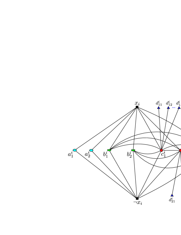
Figure 1: Gadget $G_{i}$.

Schedule.

We construct a schedule $\pi$ for $G$ under which $opt(I)$ clause nodes, $N$ literal nodes and all $N(4+9L)$ nodes in $\cup_{i=1}^{N}A_{i}\cup B_{i}\cup D_{i}$ choose $\mathcal{N}$, which proves the following lemma.

Lemma A.1.

$opt(G)\geq opt(I)+(5+9L)N.$

Proof.

Let $T$ be the set of TRUE literals in an optimal truth assignment of $I$. Then $T$ is an independent set of literal nodes in $G$ such that for each $i=1,2,\ldots,N$, exactly one of $x_{i}$ and $\neg x_{i}$ is contained in $T$. The schedule $\pi$ proceeds in two stages.

In the first stage, $\pi$ schedules the (literal) nodes in $T$ and then the $M$ clause nodes. Since $T$ is independent, all its nodes choose $\mathcal{Y}$. Therefore, the $opt(I)$ clause nodes (which correspond to the satisfied clauses) all choose $\mathcal{N}$.

In the second stage, $\pi$ schedules gadgets one after another in an arbitrary order. For each gadget $G_{i}$, let $x$ be $x_{i}$ or $\neg x_{i}$ whichever belongs to $T$ and thus has chosen $\mathcal{Y}$. Within subnetwork $G_{i}$, schedule $\pi$ proceeds in five steps. (1) $\pi$ schedules the nodes in the independent set $A_{i}\cup B_{i}$ first; obviously these nodes all choose $\mathcal{N}$ due to their common neighbor $x$. (2) Then $\pi$ schedules $c^{i}_{1}$, $c^{i}_{2}$, $\ldots$, $c^{i}_{8}$ in this order. When $c^{i}_{1}$ is scheduled, she has exactly one neighbor choosing $\mathcal{Y}$, i.e., $x$, and two neighbors choosing $\mathcal{N}$, i.e., $b^{i}_{1},b^{i}_{2}$. Therefore $c^{i}_{1}$ chooses $\mathcal{Y}$. Inductively, for $k=2,3,\ldots,8$, given $\pi[c^{i}_{k-1}]=\mathcal{Y}$, when $\pi$ schedules $c^{i}_{k}$, the node $c^{i}_{k}$ has exactly two neighbors choosing $\mathcal{Y}$ (i.e., $x,c^{i}_{k-1}$) and exactly two neighbors choosing $\mathcal{N}$ (i.e., $b^{i}_{1},b^{i}_{2}$), which implies $\pi[c^{i}_{k}]=\mathcal{Y}$. (3) Next, $\pi$ schedules $\neg x$. At that time, inside $G_{i}$ node $\neg x$ has exactly $|A_{i}\cup B_{i}|=4$ neighbors choosing $\mathcal{N}$ and $|C_{i}|-1=8$ neighbors choosing $\mathcal{Y}$; outside $G_{i}$, node $\neg x$ has at most 3 neighbors. It follows that $\neg x$ chooses $\mathcal{N}$. (4) Now $\pi$ schedules $c^{i}_{9}$. At this time $c^{i}_{9}$ has exactly three neighbors choosing $\mathcal{Y}$ (i.e., $x$, $c^{i}_{8}$, $c^{i}_{1}$) and exactly three neighbors choosing $\mathcal{N}$ (i.e., $b^{i}_{1},b^{i}_{2},\neg x$). Therefore $c^{i}_{9}$ chooses $\mathcal{Y}$ as all other nodes of $C_{i}$ do. (5) In the last step, $\pi$ schedules the nodes in $D_{i}$, all with decisions $\mathcal{N}$.

Since $\pi$ schedules each $G_{i}$ with $|A_{i}|+|B_{i}|+|\{\neg x\}|+|D_{i}|=5+9L$ decisions of $\mathcal{N}$, it follows that $\pi$ schedules $G$ with $opt(I)+N(5+9L)$ decisions of $\mathcal{N}$, establishing the lemma. ∎

Assignment.

Let $\pi^{*}$ be a schedule for $G$ that leads to a maximum number $opt(G)$ of $\mathcal{N}$ decisions. To establish the reverse inequality of the one in Lemma A.1, we will construct a truth assignment for $I$ based on $\pi^{*}$’s schedule of literal node. Notice from Lemma A.1, $|V|=M+(15+9L)N$ and $L=10N+M$ that $opt(G)>N(5+9L)=|V|-L$.

Claim 8.

$\pi^{*}$ schedules all $9N$ nodes in $\cup_{i=1}^{N}C_{i}$ with decision $\mathcal{Y}$, and therefore (by the maximality of $opt(G)$) schedules all nodes in $D^{i}_{k}$ after $c_{k}^{i}$ with $\mathcal{N}$ decisions for any $i=1,2,\ldots,N$ and $k=1,2,\ldots,9$.

Proof.

If $\pi^{*}$ schedules some $c^{i}_{k}\in C_{i}$ with decision $\mathcal{N}$, then all the $L$ nodes $d^{i}_{k1},d^{i}_{k2},\ldots,d^{i}_{kL}$ choose $\mathcal{Y}$ under $\pi^{*}$, a contradiction to $opt(G)>|V|-L$. ∎

Claim 9.

Let $T^{*}$ be the set of literal nodes who choose $\mathcal{Y}$ under $\pi^{*}$. For each $i=1,2,\ldots,N$, at most one of $x_{i}$ and $\neg x_{i}$ is contained in $T^{*}$.

Proof.

Suppose that $\pi^{*}$ schedules some literal node $x\in\{x_{i},\neg x_{i}\}$ with decision $\mathcal{Y}$ for some $i\in\{1,2,\ldots,N\}$. Note that $x$ has at most $16$ neighbors; 9 of them belong to $C_{i}$ and are scheduled by $\pi^{*}$ with decisions $\mathcal{Y}$ (see Claim 8). It must be the case that $\pi^{*}$ schedules $x$ before the last scheduled node $c\in C_{i}$. At the time $\pi^{*}$ schedules $c$, by Claim 8, $c$ has exactly two neighbors in $C_{i}$ choosing $\mathcal{Y}$, and has no neighbor in $D_{i}$ that has been scheduled. The other four neighbors of $c$ are $x,\neg x,b_{1},b_{2}$. It follows from $\pi^{*}[c]=\mathcal{Y}$ and $\pi^{*}[x]=\mathcal{Y}$ that $\pi^{*}$ schedules $\neg x$, $b_{1}$ and $b_{2}$ before $c$ with decision $\mathcal{N}$. ∎

Lemma A.2.

$opt(G)\leq opt(I)+(5+9L)N$.

Proof.

By Claim 9, $\{1,2,\ldots,N\}$ is the disjoint union of two sets $K_{1}$ and $K_{2}$ such that $\pi^{*}$ schedules exactly one of $x_{i}$ and $\neg x_{i}$ with $\mathcal{N}$ for every $i\in K_{1}$, and schedules $x_{i}$ and $\neg x_{i}$ with $\mathcal{N}$ for every $i\in K_{2}$. Note that $|K_{1}|=|T^{*}|$, $|T^{*}|+|K_{2}|=N$ and $\pi^{*}$ schedules all nodes in $\{a_{1}^{i},a_{2}^{i}:i\in K_{2}\}$ with $\mathcal{Y}$.

Define a truth assignment of $I$ by setting a literal to be TRUE if and only if it belongs to $T^{*}\cup\{x_{i}:i\in K_{2}\}$. Note that any clause node $y$ with decision $\pi^{*}[y]=\mathcal{N}$ must have a neighbor (which is a literal node) choosing $\mathcal{Y}$ under $\pi^{*}$. This neighbor thus belongs to $T^{*}$. Thus clause $y$ is satisfied by the truth assignment. It follows that $\pi^{*}$ schedules at most $opt(I)$ clause nodes with $\mathcal{N}$. From Claim 8 we deduce that

$$opt(G) \leq |V\setminus\cup_{j=1}^{N}C_{j}\setminus T^{*}\setminus\{a_{1}^{i},a_{2}^{i}:i\in K_{2}\}\setminus\{y_{j}:j=1,2,\ldots,M\}|+opt(I)$$

$$= |V|-9N-|T^{*}|-2|K_{2}|-M+opt(I)$$

$$= |V|-10N-|K_{2}|-M+opt(I).$$

It follows from $|V|\!=\!M+(15+9L)N$ that $opt(G)\!\leq\!(5+9L)N+opt(I)-|K_{2}|$. ∎

Appendix B Time complexity in Theorem 2.5

Preprocessing.

Initially, we set graph $H$ to be $G=(V,E)$, We find in $O(m)$ time a maximal independent set $X$ of $H$, and set $Y:=V\setminus X$.

To find $X_{i},Y_{i}$, $i=0,1,2,\ldots,\ell$, we will modify $H$ step by step via removing some nodes (together with their incident links). At any step, we call a node of $H$ an $X$-node (resp. a $Y$ node) if this node belongs to $X$ (resp. $Y$). In $H$, a $Y$-node is critical if it is adjacent to a pendant $X$-node. Any single non-critical node can be removed from $H$ without destroying the $Y$-node domination of $X$-nodes.

Inductively, we consider $i=0,1,\ldots,\ell$ in this order. The $i$-th stage of the process starts with $H=G_{i}$ and $Y_{i}=\emptyset$. Subsequently,

• whenever $H$ has a non-critical $Y$-node $v$, we remove $v$ from $H$, add $v$ to $Y_{i}$, and update $H$.

The repetition finishes when all $Y$-nodes in $H$ are critical. At that time, the $i$-th stage finishes with

• outputting $Y_{i}$ and $X_{i+1}$ the set of pendant nodes;

• removing all nodes of $X_{i+1}$ from $H$, and updates $H$ which gives $G_{i+1}=H$.

Running time.

Next we show that all the above $\ell+1$ stages finish in $O(m)$ time. At the initiation step, in $O(m)$ time we find the set of pendant $X$-nodes, and the set of non-critical $Y$-nodes of $H$, where $H=G$.

As our preprocessing proceeds, when we remove a $Y$-node $v$ from $H$, we update $H$ by modifying the adjacency list representation of $H$, and

• updating the degrees of all $X$-nodes;

• updating the set of pendant $X$-nodes (using the degrees updated);

• updating the set of non-critical $Y$-nodes (using the pendant $X$-nodes created).

These can be done in $O(d(v))$ time, where $d(v)$ is the degree of $v$ in $G$. Thus in the whole process, the removals of $Y$-nodes and their corresponding update in (i) take $O(\sum_{v\in Y}d(v))=O(|E|)=O(m)$ time.

When we remove all pendant $X$-nodes from $H$, we update by modifying the adjacency list representation of $H$,

• updating the set of pendant $X$-nodes (i.e., setting it to be empty);

• updating the set of non-critical $Y$-nodes (i.e., enlarging it by the unique $Y$-neighbors of the removed $X$-nodes).

Hence throughout removals of pendant $X$-nodes and their corresponding update in (iii) takes $O(|X|)=O(n)$ time.

Since throughout the process, we have an updated set of non-critical $Y$-nodes at hand, at any time, finding a non-critical node of $H$ takes $O(1)$ time. The overall running time of (i) is $O(m)$, so is that of (iii). Note that all $X_{i},Y_{i}$, $i=1,2,\ldots,\ell$, are mutually disjoint. Hence, overall, (ii) takes $O(n)$ time. Recall that $X_{0}=\emptyset$. We have the following results.

Lemma B.1.

All $X_{i}$ and $Y_{i}$, $i=0,1,\ldots,\ell$ can be found in $O(m)$ time.∎

Since $G_{i}\subseteq G_{i-1}$ for $i=\ell,\ell-1,\ldots,1$, the refinement of Algorithm 1, stated in Algorithm 2, runs $O(n^{2})$ time.

References

- [1] T. Adachi, Third-degree price discrimination, consumption externalities and social welfare, Economica 72 (2005) 171-178.
- [2] K. Apt, E. Markakis, Diffusion in social networks with competing products, In Proc. 4th international conference on Algorithmic game theory, pp.212-223, 2011
- [3] A. Borodin, Y. Filmus, and J. Oren, Threshold models for competitive influence in social networks, In Proc. 6th International Workshop on Internet and Network Economics, pp.539-550, 2010
- [4] Y. Bramoulle, Anti-coordination and social interactions. Games and Economic Behavior, 58 (2007) 30-49.
- [5] Z. Cao, X. Yang, A note on anti-coordination and social interactions, Journal of Combinatorial Optimization. 2012, online first, DOI: 10.1007/s10878-012-9486-7
- [6] D.M. Chiang, C. Teng, Consumption externalities: review and future research opportunities, Electroinic Commerce Studies 3 (2005) 15-38.
- [7] F. Chierichetti, J. Kleinberg, A. Panconesi, How to schedule a cascade in an arbitrary graph, In Proc. 13th ACM Conference on Electronic Commerce, pp.355-368, 2012
- [8] S. Goyal, M. Kearns, Competitive contagion in networks, In Proc. 44th Symposium on Theory of Computing, pp.759-774, 2012.
- [9] R.G. Holcombe, R.S. Sobel, Consumption externalities and economic welfare, Eastern Economic Journal 26 (2000)157-170.
- [10] M.O. Jackson, Social and economic networks. Princeton University Press, Princeton, NJ, 2008.
- [11] N. van Nes, Understanding replacement behaviour and exploring design solutions, in Longer Lasting Products: Alternatives to the Throwaway Society, T. Cooper (ed), 2010.
- [12] C.H. Papadimitriou, M. Yannakakis, Optimization, approximation, and complexity classes, Journal of Computer and System Science 43 (1991) 425-440.
- [13] J. Zabin, G. Brebach. Precision Marketing: The New Rules for Attracting, Retaining and Leveraging Profitable Customers. John Wiley & Sons, Inc., Hoboken, 2004.