Time-dependent Landauer–Büttiker formula for transient dynamics

Abstract

We solve analytically the Kadanoff–Baym equations for a noninteracting junction connected to an arbitrary number of noninteracting wide-band terminals. The initial equilibrium state is properly described by the addition of an imaginary track to the time contour. From the solution we obtain the time-dependent electron densities and currents within the junction. The final results are analytic expressions as a function of time, and therefore no time propagation is needed — either in transient or in steady-state regimes. We further present and discuss some applications of the obtained formulae.

1 Introduction

The Landauer–Büttiker formula [1, 2] provides an intuitive physical picture of the steady-state current flowing in a multi-terminal junction and it is simple to implement. First one calculates the steady-state current $I_{\alpha\beta}$ in terminal $\beta$ carried by the scattering states originating from terminal $\alpha\neq\beta$ and populated according to the electrochemical potential $\mu_{\alpha}$. Then one sums the difference $I_{\alpha\beta}-I_{\beta\alpha}$ between the currents flowing in and out terminal $\beta$ over all terminals $\alpha\neq\beta$. This gives the steady-state current $I_{\beta}$ in terminal $\beta$.

The first microscopic derivation (based on the time-dependent Schrödinger equation) of the Landauer–Büttiker formula was given by Caroli and co-workers [3, 4]. They considered the terminals initially uncontacted and in equilibrium at different chemical potentials. Then they switched on the contacts and derived the Landauer–Büttiker formula as the long-time limit of the expectation value at time $t$ of the current operator. We will refer to this procedure as the partitioned approach.

An alternative approach, more akin to the the way the experiments are carried out, was proposed by Cini about a decade later [5]. He considered the system initially contacted and in equilibrium at a unique chemical potential and then drove the system out of equilibrium by applying a bias voltage between the terminals. We will refer to this procedure as the partion-free approach. In both approaches one recovers the Landauer–Büttiker formula due to the loss of memory of the initial preparation [6].

The microscopic derivation of the Landauer–Büttiker formula requires the evaluation of the expectation value $I_{\beta}(t)=\langle\Psi(t)|\hat{I}_{\beta}|\Psi(t)\rangle$ where $|\Psi(t)\rangle$ is the many-body state of the system at time $t$ and $\hat{I}_{\beta}$ is the current operator. Since the electrons are noninteracting this expectation value can be rewritten as the sum over all occupied one-particle states $|\psi_{k}(t)\rangle={\mathrm{e}}^{-{\mathrm{i}}\hat{h}t}|\psi_{k}\rangle$ of $\langle\psi_{k}(t)|\hat{I}_{\beta}|\psi_{k}(t)\rangle$. Here $\hat{h}$ is the Hamiltonian of the contacted and biased system whereas $|\psi_{k}\rangle$ are the eigenstates of the Hamiltonian $\hat{h}_{0}$ which describes either the non-biased uncontacted system (in the partitioned approach) or the non-biased contacted system (in the partition-free approach). For the evaluation of $\langle\psi_{k}(t)|\hat{I}_{\beta}|\psi_{k}(t)\rangle$ one could naively insert a complete set of eigenstates $|\phi_{q}\rangle$ of $\hat{h}$ and evaluate the overlaps $\langle\psi_{k}|\phi_{q}\rangle$. This procedure is, however, numerically lengthy and unstable due to the singular $\delta$-like contribution to the overlaps. The calculation of $I_{\beta}(t)$ is most easily carried out using nonequilibrium Green’s functions [7, 8]. This mathematical tool when applied to quantum transport in multi-terminal junctions provides a natural framework to calculate the current at all times and not only at the steady state.

In fact, there have been several attempts to generalize the Landauer–Büttiker formula to the time domain. Here we mention the work of Pastawski who derived a formula for $I_{\beta}(t)$ using the partitioned approach in the linear response and adiabatic regime [9]. An important step forward in the calculation of $I_{\beta}(t)$ was done by Jauho et al. [8]. These authors used the partitioned approach to write $I_{\beta}(t)$ as a double integral (over time and energy) of the trace over the junction degrees of freedom of a calculable combination of Green’s functions in the same region. In the special case of terminals with a wide band and of junctions with one single level it is possible to perform the time-integral and obtain a time-dependent version of the Landauer–Büttiker formula. This formula was then derived in Ref. [6] using the partition-free approach, thus confirming the loss of memory of the initial preparation.

The derivation of a time-dependent Landauer–Büttiker formula for arbitrary junctions would be extremely useful to interpret the oscillations and damping times typically observed in the transient current after the sudden switch on of a bias. A progress in this direction was done in Ref. [10] where the authors derived a time-dependent Landauer–Büttiker formula for the spin current of a single-level junction.

In this work we generalize the results of Ref. [10] to junctions of any shape and dimensions using the wide-band limit approximation (WBLA) for noninteracting electrons (Secs. 2 and 3). Furthermore we also derive a general formula for the time-dependent one-particle density matrix which can be used to calculate the local density and current density. We will work in the partition-free approach which is conceptually easier since it does not involve the subtle issue of different chemical potentials in equilibrium. The final formulae for the current and the one-particle density matrix have the merit of elucidating the relative importance of the electronic transitions at a certain time. As an illustration we will use these formulae to calculate the transient response of a ring-shaped junction (Sec. 4).

2 Assumptions and set-up

We investigate the following quantum transport setup: An arbitrary number of metallic leads ($\alpha$) acting as charge-carrier reservoirs are connected to a lattice network acting as a molecular device ($C$). We assume that the electron transport is ballistic and therefore neglect the electron–electron interactions. We will also assume that the energy eigenvalues of the Hamiltonian of the molecular device are well inside the continuous energy spectrum of the leads and use the WBLA.

The described set-up is characterized by the following Hamiltonian:

$${\hat{H}}=\sum_{k\alpha,\sigma}\epsilon_{k\alpha}^{{\color[rgb]{1,1,1}\dagger}}\hat{n}_{k\alpha,\sigma}^{{\color[rgb]{1,1,1}\dagger}}+\sum_{mn,\sigma}T_{mn}^{{\color[rgb]{1,1,1}\dagger}}\hat{d}_{m,\sigma}^{\dagger}\hat{d}_{n,\sigma}^{{\color[rgb]{1,1,1}\dagger}}+\sum_{mk\alpha,\sigma}\left[T_{mk\alpha}^{{\color[rgb]{1,1,1}\dagger}}\hat{d}_{m,\sigma}^{\dagger}\hat{d}_{k\alpha,\sigma}^{{\color[rgb]{1,1,1}\dagger}}+T_{k\alpha m}^{{\color[rgb]{1,1,1}\dagger}}\hat{d}_{k\alpha,\sigma}^{\dagger}\hat{d}_{m,\sigma}^{{\color[rgb]{1,1,1}\dagger}}\right]\ .$$ (1)

The first term accounts for the leads with $k\alpha$ indexing the $k$:th basis function of the $\alpha=1,2,3,\ldots$ lead. The single-particle spectrum of the leads is $\epsilon_{k\alpha}$ and the number operator in the leads is expressed in terms of the creation and annihilation operators as $\hat{n}_{k\alpha,\sigma}^{{\color[rgb]{1,1,1}\dagger}}=\hat{d}_{k\alpha,\sigma}^{\dagger}\hat{d}_{k\alpha,\sigma}^{{\color[rgb]{1,1,1}\dagger}}$, with $\sigma$ the spin index. The second term is for the molecular device, or central region, (indices $m$ and $n$) with creation and annihilation operators $\hat{d}_{m,\sigma}^{\dagger}$ and $\hat{d}_{m,\sigma}^{{\color[rgb]{1,1,1}\dagger}}$ and hoppings $T_{mn}$ between sites $m$ and $n$. The last term is for the coupling between the central region and the leads with hoppings $T_{mk\alpha}$.

At times $t<t_{0}$ the system is in thermal equilibrium at inverse temperature $\beta$ and chemical potential $\mu$, the density matrix having the form $\hat{\rho}=\frac{1}{\mathcal{Z}}{\mathrm{e}}^{-\beta({\hat{H}}-\mu{\hat{N}})}$ where $\mathcal{Z}$ is the grand-canonical partition function. At $t=t_{0}$ the lead energy levels are suddenly shifted by some constant value, $\epsilon_{k\alpha}\to\epsilon_{k\alpha}+V_{\alpha}$, to model the sudden switch-on of an external bias voltage in the $\alpha$:th lead. This means that the system is driven out of equilibrium and charge carriers start to flow through the central region. To calculate the time-dependent current we use the equations of motion for the one-particle Green’s function on the Keldysh contour $\gamma_{\text{K}}$. This quantity is defined as the ensemble average of the contour-ordered product of particle creation and annihilation operators in the Heisenberg picture

$$G_{rs}(z,z^{\prime})=-{\mathrm{i}}\langle\mathcal{T_{\gamma_{\text{K}}}}[\hat{d}_{r,\mathrm{H}}^{{\color[rgb]{1,1,1}\dagger}}(z)\hat{d}_{s,\mathrm{H}}^{\dagger}(z^{\prime})]\rangle$$ (2)

where the indices $r$, $s$ can be either indices in the leads or in the central region and the variables $z$, $z^{\prime}$ run on the contour. The matrix $G$ with matrix elements $G_{rs}$ satisfies the equations of motion

$$\left[{\mathrm{i}}\frac{{\mathrm{d}}}{{\mathrm{d}}z}-\mbox{\boldmath$h$}(z)\right]\mbox{\boldmath$G$}(z,z^{\prime}) = \delta(z,z^{\prime})\mbox{\boldmath$1$}\ ,$$ (3)

$$\mbox{\boldmath$G$}(z,z^{\prime})\left[-{\mathrm{i}}\frac{\stackrel{{\scriptstyle\leftarrow}}{{{\mathrm{d}}}}}{{\mathrm{d}}z^{\prime}}-\mbox{\boldmath$h$}(z^{\prime})\right] = \delta(z,z^{\prime})\mbox{\boldmath$1$}\ ,$$ (4)

with Kubo–Martin–Schwinger (KMS) boundary conditions. Here $\mbox{\boldmath$h$}(z)$ is the single-particle Hamiltonian. In the basis $k\alpha$ and $m$ the matrix $h$ has the following block structure

$$\mbox{\boldmath$h$}=\begin{pmatrix}h_{11}&0&0&\cdots&h_{1C}\\ 0&h_{22}&0&\cdots&h_{2C}\\ 0&0&h_{33}&\cdots&h_{3C}\\ \vdots&\vdots&\vdots&\ddots&\vdots\\ h_{C1}&h_{C2}&h_{C3}&\cdots&h_{CC}\end{pmatrix}\ ,$$ (5)

where $(h_{\alpha\alpha^{\prime}})_{kk^{\prime}}=\delta_{\alpha\alpha^{\prime}}\delta_{kk^{\prime}}\epsilon_{k\alpha}$ corresponds to the leads, $(h_{\alpha C})_{km}=T_{k\alpha m}$ is the coupling part, and $(h_{CC})_{mn}=T_{mn}$ accounts for the central region. As the system is initially in thermal equilibrium we have that for $z$ on the vertical track of the contour $\epsilon_{k\alpha}(z)=\epsilon_{k\alpha}-\mu$, $T_{k\alpha m}(z)=T_{k\alpha m}$ and $T_{mn}(z)=T_{mn}-\mu\delta_{mn}$. On the other hand for $z$ on the horizontal branches we have $\epsilon_{k\alpha}(z)=\epsilon_{k\alpha}+V_{\alpha}$, $T_{k\alpha m}(z)=T_{k\alpha m}$ and $T_{mn}(z)=T_{mn}$. Due to the coupling between the central region and the leads the matrix $G$ has nonvanishing entries everywhere

$$\mbox{\boldmath$G$}=\begin{pmatrix}G_{11}&\cdots&G_{1C}\\ \vdots&\ddots&\vdots\\ G_{C1}&\cdots&G_{CC}\end{pmatrix}.$$ (6)

In the next Section we solve the equations of motion (3) and (4) for the Green’s function $G_{CC}$ projected in the central region.

3 Derivation of the time-dependent density and current

3.1 Projecting the equation of motion

We project the equation of motion (3) onto regions $CC$ and $\alpha C$. The equation for $G_{\alpha C}$ can be integrated using the Green’s function $g_{\alpha\alpha}(z,z^{\prime})$ of the isolated $\alpha$:th reservoir. This Green’s function solves the equation of motion $\left[{\mathrm{i}}\frac{{\mathrm{d}}}{{\mathrm{d}}z}-h_{\alpha\alpha}\right]g_{\alpha\alpha}(z,z^{\prime})=\delta(z,z^{\prime})$ as well as the adjoint equation with KMS boundary conditions. Introducing the embedding self-energy (with indices in region $C$)

$$\mbox{$\mathit{\Sigma}$}_{\text{em}}(z,z^{\prime})=\sum_{\alpha}\Sigma_{\alpha}(z,z^{\prime})\quad;\quad\Sigma_{\alpha}(z,z^{\prime})=h_{C\alpha}g_{\alpha\alpha}(z,z^{\prime})h_{\alpha C}$$ (7)

we obtain the equation of motion for the Green’s function of the central region (the subscripts $CC$ are omitted from now on)

$$\left[{\mathrm{i}}\frac{{\mathrm{d}}}{{\mathrm{d}}z}-h\right]G(z,z^{\prime})=\delta(z,z^{\prime})+\int_{\gamma_{\text{K}}}\!\!\!{\mathrm{d}}\bar{z}\mbox{$\mathit{\Sigma}$}_{\text{em}}(z,\bar{z})G(\bar{z},z^{\prime})$$ (8)

The adjoint equation of motion can be derived similarly and read [11]

$$G(z,z^{\prime})\left[-{\mathrm{i}}\frac{\stackrel{{\scriptstyle\leftarrow}}{{{\mathrm{d}}}}}{{\mathrm{d}}z^{\prime}}-h\right]=\delta(z,z^{\prime})+\int_{\gamma_{\text{K}}}\!\!\!{\mathrm{d}}\bar{z}G(z,\bar{z})\mbox{$\mathit{\Sigma}$}_{\text{em}}(\bar{z},z^{\prime})\ .$$ (9)

The embedded equations of motion for $G$ have the same structure as the Kadanoff–Baym equations (KBE), the difference being that the many-body self-energy is replaced by the embedding self-energy. In the case of interacting electrons with an interaction only in the central region Eqs. (8) and (9) are modified by the addition of the many-body self-energy $\mathit{\Sigma}$ to the embedding self-energy $\mbox{$\mathit{\Sigma}$}_{\text{em}}$, i.e., $\mbox{$\mathit{\Sigma}$}_{\text{em}}\rightarrow\mbox{$\mathit{\Sigma}$}_{\text{em}}+\mbox{$\mathit{\Sigma}$}$. Since $\mbox{$\mathit{\Sigma}$}=\mbox{$\mathit{\Sigma}$}[G]$ is a functional of the Green’s function in region $C$ the embedded equations of motion in the interacting case constitute a closed set of integro-differential, nonlinear equations for $G$ [11]. The simplification brought by the absence of interactions is that the KBE (8) and (9) are linear in $G$ since the embedding self-energy is completely specified by the parameters of the Hamiltonian.

The density and current density can be extracted from the lesser component of the Green’s function at equal time. We denote by $z=t_{-}$ the contour point on the forward branch, $z=t_{+}$ the contour point on the backward branch and $z=t_{0}-{\mathrm{i}}\tau$ the contour point on the vertical track. The Keldysh components lesser ($<$), greater ($>$), retarded (R), advanced (A), left ($\lceil$), right ($\rceil$) and Matsubara (M) of a function $k(z,z^{\prime})$ on the contour are defined according to [12]

$$k^{<}(t,t^{\prime}) = k(t_{-},t^{\prime}_{+})$$ (10)

$$k^{>}(t,t^{\prime}) = k(t_{+},t^{\prime}_{-})$$ (11)

$$k^{\rm R}(t,t^{\prime}) = +\theta(t-t^{\prime})\left[k^{>}(t,t^{\prime})-k^{<}(t,t^{\prime})\right]$$ (12)

$$k^{\rm A}(t,t^{\prime}) = -\theta(t^{\prime}-t)\left[k^{>}(t,t^{\prime})-k^{<}(t,t^{\prime})\right]$$ (13)

$$k^{\lceil}(\tau,t^{\prime}) = k(t_{0}-{\mathrm{i}}\tau,t^{\prime})$$ (14)

$$k^{\rceil}(t,\tau) = k(t,t_{0}-{\mathrm{i}}\tau)$$ (15)

$$k^{\rm M}(\tau,\tau^{\prime}) = k(t_{0}-{\mathrm{i}}\tau,t_{0}-{\mathrm{i}}\tau^{\prime})$$ (16)

To generate an equation for $G^{<}$ we subtract Eq. (9) from Eq. (8) and set $z=t_{-}$, $z^{\prime}=t_{+}^{\prime}$. Taking into account that $h(z)=h$ is independent of $z$ for $z$ on the horizontal branches we get at equal time

$${\mathrm{i}}\frac{{\mathrm{d}}}{{\mathrm{d}}t}G^{<}(t,t)-\left[{h},{G^{<}(t,t)}\right] = \left[\mbox{$\mathit{\Sigma}$}_{\text{em}}^{\text{R}}\cdot G^{<}-G^{\text{R}}\cdot\mbox{$\mathit{\Sigma}$}_{\text{em}}^{<}+\mbox{$\mathit{\Sigma}$}_{\text{em}}^{<}\cdot G^{\text{A}}-G^{<}\cdot\mbox{$\mathit{\Sigma}$}_{\text{em}}^{\text{A}}\right](t,t)$$ (17)

$$+ \left[\mbox{$\mathit{\Sigma}$}_{\text{em}}^{\rceil}\star G^{\lceil}-G^{\rceil}\star\mbox{$\mathit{\Sigma}$}_{\text{em}}^{\lceil}\right](t,t)\ ,$$

where we defined $\left[f\cdot g\right](t,t^{\prime})=\int_{t_{0}}^{\infty}{\mathrm{d}}\bar{t}f(t,\bar{t})g(\bar{t},t^{\prime})$ and $\left[f\star g\right](t,t^{\prime})=-{\mathrm{i}}\int_{0}^{\beta}{\mathrm{d}}\tau f(t,\tau)g(\tau,t^{\prime})$. Equation (17) can also be written as

$${\mathrm{i}}\frac{{\mathrm{d}}}{{\mathrm{d}}t}G^{<}(t,t)-\left[{h},{G^{<}(t,t)}\right]=-\left[G^{\text{R}}\cdot\mbox{$\mathit{\Sigma}$}_{\text{em}}^{<}+G^{<}\cdot\mbox{$\mathit{\Sigma}$}_{\text{em}}^{\text{A}}+G^{\rceil}\star\mbox{$\mathit{\Sigma}$}_{\text{em}}^{\lceil}\right](t,t)+\text{h.c.}$$ (18)

where we used the properties of $G$ and $\mbox{$\mathit{\Sigma}$}_{\text{em}}$ under complex conjugation [12].

Let us comment Eq. (18) briefly. Setting the right-hand side to zero we see that Eq. (18) reduces to the Liouville equation for the one-particle density matrix $\rho=-{\mathrm{i}}G$ of the isolated central region. Thus the embedding self-energy accounts for the openness of region $C$. The first term inside the square brackets is a convolution between the propagator in region $C$, $G^{\text{R}}$, and $\mbox{$\mathit{\Sigma}$}_{\text{em}}^{<}$. Since $\mbox{$\mathit{\Sigma}$}_{\text{em}}^{<}$ is proportional to the probability of finding an electron in the leads this term can be interpreted as a source term, i.e., a term that describes the injection of electrons into region $C$. The second term has the opposite structure: a propagator in the leads, $\mbox{$\mathit{\Sigma}$}_{\text{em}}^{\rm A}$, is convoluted with $G^{<}$ which is propotional to the probability of finding an electron in region $C$. Thus this term can be interpreted as a drain term and is responsible for damping and equilibration effects. The last term inside the square brackets accounts for the initial preparation of the system. In the partioned approach this term would be zero since the hopping integrals $T_{k\alpha m}=0$ in equilibrium. However, in the partition-free approach this term is nonzero and accounts for the initial coupling of the central region to the leads.

More generally convolutions along the vertical track carry information on the initial preparation of the system. For instance for a system of interacting electrons we can either start with a noninteracting system and then switch on the interaction in real time or we can start with a system already interacting. In the latter case the many-body self-energy is nonvanishing on the vertical track and the convolution $G\star\mbox{$\mathit{\Sigma}$}$ accounts for the effects of initial correlations.

3.2 Self-energy and Green’s function calculations

The solution of Eq. (18) requires first to calculate the Matsubara component $G^{\text{M}}$, and then from $G^{\text{M}}$ the right and left component $G^{\rceil}$ and $G^{\lceil}$. The Matsubara component $G^{\text{M}}$ can be determined from the retarded/advanced components by analytic continuation, see below. Since the equations for $G^{\text{M}}$, $G^{\rceil}$ and $G^{\lceil}$ contain the embedding self-energy the preliminary step is to obtain an expression for $\mbox{$\mathit{\Sigma}$}_{\text{em}}$.

Having a time-independent Hamiltonian (on the horizontal branches of the contour) the retarded/advanced components of the self-energy depend only on the time difference

$$\mbox{$\mathit{\Sigma}$}^{\text{A}}_{\alpha,mn}(t,t^{\prime})={\int\frac{{\mathrm{d}}\omega}{2\pi}}{\mathrm{e}}^{-{\mathrm{i}}{\omega}(t-t^{\prime})}\sum_{k}T_{mk\alpha}\,g_{k\alpha}^{\mathrm{A}}({\omega})\,T_{k\alpha n}$$ (19)

where $g_{k\alpha}$ is the diagonal element of the Green’s function $g_{\alpha\alpha}$ of the isolated $\alpha$:th lead, see Eq. (7). The retarded component of the self-energy is found by conjugating $\mbox{$\mathit{\Sigma}$}^{\text{R}}_{\alpha}(t,t^{\prime})=\left[\mbox{$\mathit{\Sigma}$}^{\text{A}}_{\alpha}(t^{\prime},t)\right]^{\dagger}$. According to the WBLA the Fourier transform of $\mbox{$\mathit{\Sigma}$}^{\text{A}}_{\alpha}$ is frequency independent

$$\mbox{$\mathit{\Sigma}$}^{\text{A}}_{\alpha,mn}({\omega})=\sum_{k}T_{mk\alpha}\,g_{k\alpha}^{\mathrm{A}}({\omega})\,T_{k\alpha n}=\sum_{k}T_{mk\alpha}\frac{1}{{\omega}-\epsilon_{k\alpha}-V_{\alpha}-{\mathrm{i}}\eta}T_{k\alpha n}=\frac{{\mathrm{i}}}{2}\mbox{$\mathit{\Gamma}$}_{\alpha,mn}\$$ (20)

which implies that $\mbox{$\mathit{\Sigma}$}^{\text{A}}_{\alpha}$ is also independent of the external bias voltage $V_{\alpha}$. The time-dependent self-energy of Eq. (19) is therefore

$$\mbox{$\mathit{\Sigma}$}^{\text{A}}_{\alpha,mn}(t,t^{\prime})={\int\frac{{\mathrm{d}}\omega}{2\pi}}{\mathrm{e}}^{-{\mathrm{i}}{\omega}(t-t^{\prime})}\mbox{$\mathit{\Sigma}$}^{\text{A}}_{\alpha,mn}({\omega})=\frac{{\mathrm{i}}}{2}\mbox{$\mathit{\Gamma}$}_{\alpha,mn}\delta(t-t^{\prime})\ .$$ (21)

Within the WBLA we can easily calculate the two other self-energy components in Eq. (18) (see A)

$$\mbox{$\mathit{\Sigma}$}_{\alpha,mn}^{\lceil}(\tau,t) = \mbox{$\mathit{\Gamma}$}_{\alpha,mn}\frac{1}{-{\mathrm{i}}\beta}\sum_{q}{\mathrm{e}}^{-{\omega}_{q}\tau}{\int\frac{{\mathrm{d}}\omega}{2\pi}}\frac{{\mathrm{e}}^{{\mathrm{i}}({\omega}+V_{\alpha})t}}{{\omega}_{q}-{\omega}+\mu}\ ,$$ (22)

$$\mbox{$\mathit{\Sigma}$}_{\alpha,mn}^{<}(t,t^{\prime}) = {\mathrm{i}}\mbox{$\mathit{\Gamma}$}_{\alpha,mn}{\int\frac{{\mathrm{d}}\omega}{2\pi}}f(\omega-\mu){\mathrm{e}}^{-{\mathrm{i}}({\omega}+V_{\alpha})(t-t^{\prime})}\ ,$$ (23)

where the sum over $q$ is a sum over the Matsubara frequencies ${\omega}_{q}=\frac{(2q+1)\pi}{-{\mathrm{i}}\beta}$, and the function $f$ is the Fermi function, $f({\omega})=1/[{\mathrm{e}}^{\beta{\omega}}+1]$.

Having the explicit form of the self-energy components we can derive expressions for the Green’s function. For the following calculations it is convenient to define the effective Hamiltonian $h_{\text{eff}}=h-\frac{{\mathrm{i}}}{2}\mbox{$\mathit{\Gamma}$}\ \Rightarrow\ h_{\text{eff}}^{\dagger}=h+\frac{{\mathrm{i}}}{2}\mbox{$\mathit{\Gamma}$}$, where $\mbox{$\mathit{\Gamma}$}=\sum_{\alpha}\mbox{$\mathit{\Gamma}$}_{\alpha}$. This effective Hamiltonian is therefore non-hermitean. The two Green’s function components in the square brackets of Eq. (18) read (see B)

$$G^{\rceil}(t,\tau) = {\mathrm{e}}^{-{\mathrm{i}}h_{\text{eff}}t}\Big{[}G^{\text{M}}(0,\tau)-\int_{0}^{t}{\mathrm{d}}t^{\prime}{\mathrm{e}}^{{\mathrm{i}}h_{\text{eff}}t^{\prime}}\int_{0}^{\beta}{\mathrm{d}}\bar{\tau}\mbox{$\mathit{\Sigma}$}_{\rm em}^{\rceil}(t^{\prime},\bar{\tau})G^{\text{M}}(\bar{\tau},\tau)\Big{]}\ ,$$ (24)

$$G^{\text{R}}(t,t^{\prime}) = -{\mathrm{i}}\theta(t-t^{\prime}){\mathrm{e}}^{-{\mathrm{i}}h_{\text{eff}}(t-t^{\prime})}\ ,$$ (25)

with $G^{\text{M}}$ the Matsubara Green’s function. $G^{\text{M}}$ can be obtained from $G^{\text{R}}$ and $G^{\text{A}}$ by analytic continuation since $G^{\text{M}}({\omega}_{q})=G^{\rm R}({\omega}_{q}+\mu)$ if ${\rm Im}[{\omega}_{q}]>0$ and $G^{\text{M}}({\omega}_{q})=G^{\text{A}}({\omega}_{q}+\mu)$ if ${\rm Im}[{\omega}_{q}]<0$, see B.

Now we have all ingredients to calculate the convolutions in Eq. (18). We report here the final results and refer to C for details. The three terms read

$$\left[G^{\text{R}}\cdot\mbox{$\mathit{\Sigma}$}_{\rm em}^{<}\right](t,t) = {\mathrm{i}}\sum_{\alpha}{\int\frac{{\mathrm{d}}\omega}{2\pi}}f(\omega-\mu)\left[1-{\mathrm{e}}^{{\mathrm{i}}({\omega}+V_{\alpha}-h_{\text{eff}})}\right]G^{\text{R}}({\omega}+V_{\alpha})\mbox{$\mathit{\Gamma}$}_{\alpha}\ ,$$ (26)

$$\left[G^{<}\cdot\mbox{$\mathit{\Sigma}$}^{\text{A}}_{\rm em}\right](t,t) = \frac{{\mathrm{i}}}{2}G^{<}(t,t)\mbox{$\mathit{\Gamma}$}\ ,$$ (27)

$$\left[G^{\rceil}\star\mbox{$\mathit{\Sigma}$}_{\rm em}^{\lceil}\right](t,t) = {\mathrm{i}}{\int\frac{{\mathrm{d}}\omega}{2\pi}}f(\omega-\mu)\sum_{\alpha}{\mathrm{e}}^{{\mathrm{i}}({\omega}+V_{\alpha}-h_{\text{eff}})t}G^{\text{R}}({\omega})\mbox{$\mathit{\Gamma}$}_{\alpha}\ .$$ (28)

3.3 Solving Eq. (18) for $G^{<}(t,t)$

We insert Eqs. (26), (27) and (28) into Eq. (18) and get

$${\mathrm{i}}\frac{{\mathrm{d}}}{{\mathrm{d}}t}G^{<}(t,t)-\big{[}h,G^{<}(t,t)\big{]}$$ (29)

$$= -\left\{{\mathrm{i}}\sum_{\alpha}{\int\frac{{\mathrm{d}}\omega}{2\pi}}f(\omega-\mu)\left[1-{\mathrm{e}}^{{\mathrm{i}}({\omega}+V_{\alpha}-h_{\text{eff}})t}\right]G^{\text{R}}({\omega}+V_{\alpha})\mbox{$\mathit{\Gamma}$}_{\alpha}+\frac{{\mathrm{i}}}{2}\mbox{$\mathit{\Gamma}$}G^{<}(t,t)\right.$$

$$\hskip 10.0pt+\left.{\mathrm{i}}{\int\frac{{\mathrm{d}}\omega}{2\pi}}f(\omega-\mu)\sum_{\alpha}{\mathrm{e}}^{{\mathrm{i}}({\omega}+V_{\alpha}-h_{\text{eff}})t}G^{\text{R}}({\omega})\mbox{$\mathit{\Gamma}$}_{\alpha}\right\}+\text{h.c.}$$

This is a nonhomogeneous, linear, first-order differential equation for $G^{<}(t,t)$ and, therefore, can be solved explicitly. The solution is worked out in D and reads

$$-{\mathrm{i}}G^{<}(t,t) = {\int\frac{{\mathrm{d}}\omega}{2\pi}}f(\omega-\mu)\sum_{\alpha}\Big{\{}\ A_{\alpha}({\omega}+V_{\alpha})$$ (30)

$$+ V_{\alpha}\left[{\mathrm{e}}^{{\mathrm{i}}({\omega}+V_{\alpha}-h_{\text{eff}})t}G^{\text{R}}({\omega})A_{\alpha}({\omega}+V_{\alpha})+\text{h.c.}\right]$$

$$+ V_{\alpha}^{2}{\mathrm{e}}^{-{\mathrm{i}}h_{\text{eff}}t}G^{\text{R}}({\omega})A_{\alpha}({\omega}+V_{\alpha})G^{\text{A}}({\omega}){\mathrm{e}}^{{\mathrm{i}}h_{\text{eff}}^{\dagger}t}\ \Big{\}}\ ,$$

where we introduced the partial spectral function as

$$A_{\alpha}({\omega})=G^{\text{R}}({\omega})\mbox{$\mathit{\Gamma}$}_{\alpha}G^{\text{A}}({\omega})\ .$$ (31)

The full nonequilibrium spectral function is $A({\omega})=\sum_{\alpha}A_{\alpha}({\omega})$.

Given the original complexity of the problem the final result is surprisingly compact. Equation (30) is an explicit closed formula for the equal-time $G^{<}$ or, equivalently, for the reduced one-particle density matrix. All the quantities inside the integral can be calculated separately, and no time-propagation nor self-consistency algorithms are needed. Also, we may extract several physical properties:

1. With no external bias, $V_{\alpha}=0$, only the first row contributes. This term correctly gives the equilibrium value of the equal-time $G^{<}$ since at zero bias $\sum_{\alpha}A_{\alpha}({\omega})$ is the equilibrium spectral function.

2. Both the second and the third row vanish exponentially in the long-time limit, and the equal-time $G^{<}$ approaches a unique steady-state value.

3. The transient dynamics is given by the second and the third row. By inserting a complete set of eigenstates of the effective Hamiltonian $h_{\text{eff}}$ we notice that:

   1. The second row gives rise to oscillations with frequency ${\omega}_{j}=|\mu+V_{\alpha}-\epsilon_{j}^{\text{eff}}|$ where $\epsilon_{j}^{\text{eff}}$ is the real part of the $j$:th complex eigenvalue of $h_{\text{eff}}$. These oscillations correspond to transitions between the biased Fermi level of the leads and the resonant levels of the central molecule.

   2. The third term accounts for intramolecular transitions and leads to oscillations with frequency ${\omega}_{jk}=|\epsilon_{j}^{\text{eff}}-\epsilon_{k}^{\text{eff}}|$. These oscillations are visible only if the effective Hamiltonian $h_{\text{eff}}$ does not commute with $\mbox{$\mathit{\Gamma}$}_{\alpha}$. In the case that $[h_{\text{eff}},\mbox{$\mathit{\Gamma}$}_{\alpha}]=0$ the time dependence of the third term is of the form ${\mathrm{e}}^{-{\mathrm{i}}h_{\text{eff}}t+{\mathrm{i}}h_{\text{eff}}^{\dagger}t}={\mathrm{e}}^{-\mbox{$\mathit{\Gamma}$}t}$.

3.4 Current calculation

The time-dependent current through the interface between the central region and the $\alpha$:th reservoir is calculated from the following equation [11]

$$I_{\alpha}(t)=4q\operatorname{Re}\left\{\mathrm{Tr}\left[\mbox{$\mathit{\Sigma}$}_{\alpha}^{<}\cdot G^{\text{A}}+\mbox{$\mathit{\Sigma}$}_{\alpha}^{\text{R}}\cdot G^{<}+\mbox{$\mathit{\Sigma}$}_{\alpha}^{\rceil}\star G^{\lceil}\right](t,t)\right\}\ .$$ (32)

For the terms inside Eq. (32) we proceed in the same manner as we did previously to obtain the results in Eqs. (26),  (27) and (28):

$$\left[\mbox{$\mathit{\Sigma}$}_{\alpha}^{<}\cdot G^{\text{A}}\right](t,t) = {\mathrm{i}}{\int\frac{{\mathrm{d}}\omega}{2\pi}}f(\omega-\mu)\mbox{$\mathit{\Gamma}$}_{\alpha}G^{\text{A}}({\omega}+V_{\alpha})\left[1-{\mathrm{e}}^{-{\mathrm{i}}({\omega}+V_{\alpha}-h_{\text{eff}}^{\dagger})t}\right]\ ,$$ (33)

$$\left[\mbox{$\mathit{\Sigma}$}_{\alpha}^{\text{R}}\cdot G^{<}\right](t,t) = -\frac{{\mathrm{i}}}{2}\mbox{$\mathit{\Gamma}$}_{\alpha}G^{<}(t,t)\ ,$$ (34)

$$\left[\mbox{$\mathit{\Sigma}$}_{\alpha}^{\rceil}\star G^{\lceil}\right](t,t) = {\mathrm{i}}{\int\frac{{\mathrm{d}}\omega}{2\pi}}f(\omega-\mu)\mbox{$\mathit{\Gamma}$}_{\alpha}G^{\text{A}}({\omega}){\mathrm{e}}^{-{\mathrm{i}}({\omega}+V_{\alpha}-h_{\text{eff}}^{\dagger})t}\ .$$ (35)

Inserting these results into Eq. (32) and taking into account the explicit expression for $G^{<}(t,t)$ in Eq. (30) we get

$$I_{\alpha}(t) = -2{\int\frac{{\mathrm{d}}\omega}{2\pi}}f(\omega-\mu)\sum_{\beta}\mathrm{Tr}\Big{\{}$$ (36)

$$\mbox{$\mathit{\Gamma}$}_{\alpha}G^{\text{R}}({\omega}+V_{\beta})\mbox{$\mathit{\Gamma}$}_{\beta}G^{\text{A}}({\omega}+V_{\beta})-\mbox{$\mathit{\Gamma}$}_{\alpha}G^{\text{R}}({\omega}+V_{\alpha})\mbox{$\mathit{\Gamma}$}_{\beta}G^{\text{A}}({\omega}+V_{\alpha})$$

$$+ V_{\beta}\left[\mbox{$\mathit{\Gamma}$}_{\alpha}{\mathrm{e}}^{{\mathrm{i}}({\omega}+V_{\beta}-h_{\text{eff}})t}G^{\text{R}}({\omega})\left(-{\mathrm{i}}\delta_{\alpha\beta}G^{\text{R}}({\omega}+V_{\beta})+A_{\beta}({\omega}+V_{\beta})\right)+\text{h.c.}\right]$$

$$+ V_{\beta}^{2}\mbox{$\mathit{\Gamma}$}_{\alpha}{\mathrm{e}}^{-{\mathrm{i}}h_{\text{eff}}t}G^{\text{R}}({\omega})A_{\beta}({\omega}+V_{\beta})G^{\text{A}}({\omega}){\mathrm{e}}^{{\mathrm{i}}h_{\text{eff}}^{\dagger}t}\ \Big{\}}\ .$$

The physical interpretation of the terms in Eq. (36) is similar to the one after Eq. (30). We have a steady-state part given by the first row, and a time-dependent part given by the second and the third rows. The time-dependent part vanishes exponentially in the long-time limit and the oscillations in the current have the same structure as in the reduced one-particle density matrix.

4 Results

Let us consider a six-site tight-binding ring connected to two tight-binding, semi-infinite, one-dimensional leads as shown schematically in Figs. 1 and 2.

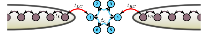
Figure 1: Six-site ring coupled symmetrically to one-dimensional TB leads.

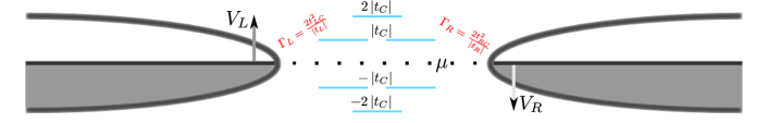
Figure 2: Schematic of the transport setup through the energy levels of the molecule.

The parameters according to the notation in the figures are $t_{C}=-2.0$ (hopping in the molecule), chemical potential $\mu=0$ and zero temperature ($\beta\to\infty$). We choose the hopping $t_{L}=t_{R}$ in the left/right lead to be much larger than any other energy scale. Then $\Sigma_{\alpha}^{\rm A}({\omega}\sim\mu)={\mathrm{i}}\,t^{2}_{\alpha C}/t_{\alpha}+O(1/t_{\alpha}^{2})$ where $t_{\alpha C}$ is the hopping between the molecule and the leads. For this situation the WBLA with $\mbox{$\mathit{\Gamma}$}_{\alpha}=2t^{2}_{\alpha C}/t_{\alpha}$ is a very good approximation. We study the weak coupling case $\Gamma_{L,R}=0.1$ and drive the system out of equilibrium by the sudden switch-on of a bias $V_{L}=V=-V_{R}$. We analyze the contribution of different terms in the charge current corresponding to different physical features as discussed below Eq. (30). In Eq. (36) the first row is ’steady state’, the second row consists of ’1st term, a’ and ’1st term, b’ and the third row is ’2nd term’. The second row is divided into two parts [$\sim G^{\text{R}}({\omega})G^{\text{R}}({\omega}+V_{\beta})$ and $\sim G^{\text{R}}({\omega})A_{\beta}({\omega}+V_{\beta})$] since they give rise to different features.

In Figs. 4 and 4 we plot the current through the right interface and see that weakly biased leads, $V=0.5$, give a negligible steady-state current. Transitions between the biased leads and the molecule are captured by the ’1st term, a’. This is confirmed by the peak in the Fourier spectrum at ${\omega}_{j}=\epsilon_{j}^{\text{eff}}\pm V$. Transitions between the molecular levels are accounted for by the ’2nd term’, as it can be seen in the Fourier transform with a peak at ${\omega}=6$. In addition to our previous observations: (1) the ’1st term, b’ also gives rise to intramolecular transitions and (2) there seems to be no intramolecular transitions at ${\omega}=2$ or ${\omega}=4$. By expanding Eq. (36) in the eigenbasis of the effective Hamiltonian and manipulating the terms further one can show that the the ’1st term, b’ contains a term of the form ${\mathrm{e}}^{-{\mathrm{i}}(\epsilon_{j}^{\text{eff}}-\epsilon_{k}^{\text{eff}})t}$ which explains the first finding. The second finding suggests that there is some underlying selection rule for some of the energy levels and hence that some levels do not participate to the transport process.

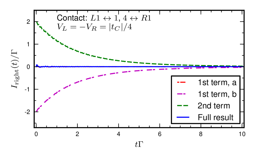
Figure 3: Different terms of the time-dependent current in units of $\Gamma$ through the right interface with symmetric coupling and weak bias.

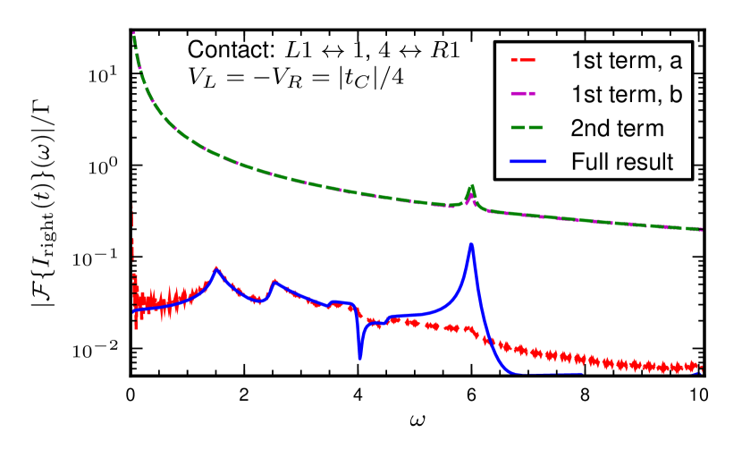
Figure 4: Absolute value of the Fourier transform of the terms of the current in units of $\Gamma$.

If we increase the bias window to cover the first molecular levels, $V=2.5$, then we see in Fig. 6 that the current has a non-zero steady-state value. Similar findings, as with weaker bias, for the possible transitions are seen in Fig. 6. We also see that there is a small bump at ${\omega}=4$ in ’1st term, b’ and ’2nd term’. Given that the setup is completely identical to the previous case, this fact is due to a second (or higher) order response since the same symmetry arguments apply.

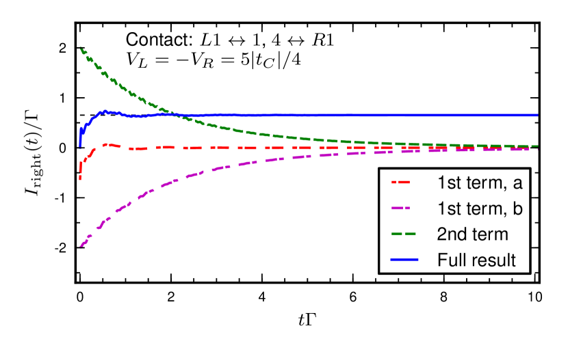
Figure 5: Different terms of the time-dependent current in units of $\Gamma$ through the right interface with symmetric coupling and strong bias.

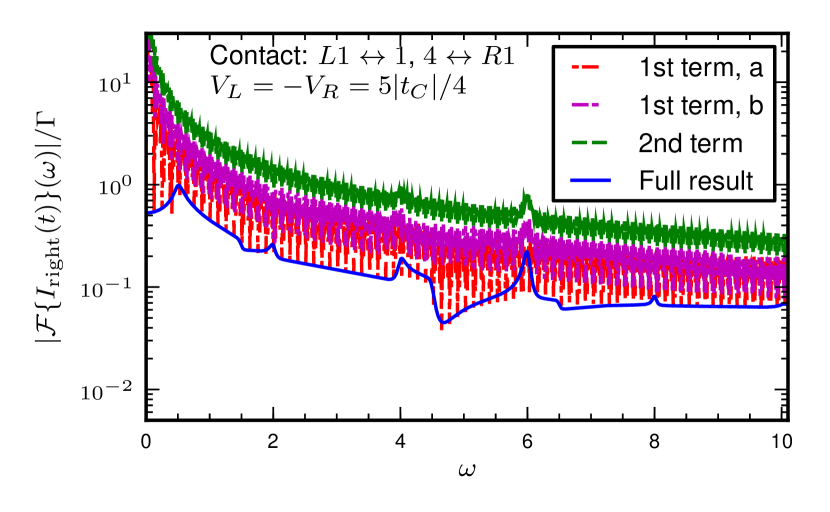
Figure 6: Absolute value of the Fourier transform of the terms of the current in units of $\Gamma$.

If we, however, distort the symmetry of the junction then also the intramolecular transitions with lower energies become visible. This is clearly seen in Figs. 8 and 8 where we connect the molecule asymmetrically to the leads (1st site to the left and 3rd site to the right, see Fig. 1).

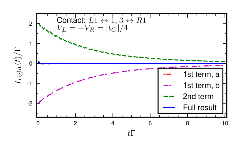
Figure 7: Different terms of the time-dependent current in units of $\Gamma$ through the right interface with asymmetric coupling and weak bias.

Figure 8: Absolute value of the Fourier transform of the terms of the current in units of $\Gamma$.

We can also break the symmetry by deforming the molecule with, for instance, one hopping (between sites $1$ and $6$) being $2t_{C}$. This splits the degenerate levels in Fig. 2 and also the corresponding intramolecular transitions can be seen in Figs. 10 and 10.

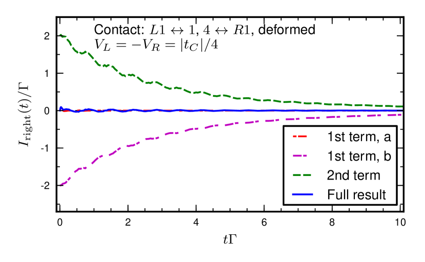
Figure 9: Different components of the time-dependent current in units of $\Gamma$ through the right interface of a deformed molecule with symmetric coupling and weak bias.

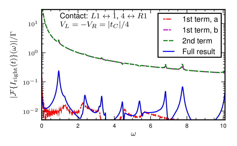
Figure 10: Absolute value of the Fourier transform of the terms of the current in units of $\Gamma$.

As the contributions from different terms sum up to the total current we can plot the full results for, e.g., the right current of the symmetrically coupled molecule against, e.g., the bias or the coupling strength. In Figs. 14, 14, 14 and 14 we display the full results. The transient dynamics is visualized better but distinguishing between the different contributions is more complicated. In Fig. 14 and 14 the axes are not scaled due to varying $\Gamma$. It is clear that by increasing the bias window more levels open up for transport and therefore the steady-state current grows. The oscillation frequencies corresponding to transitions between molecular levels remain unchanged while the oscillation frequencies corresponding to transitions between the molecule and the leads vary (peak shift). By increasing $\Gamma$, and hence by widening the resonances, electrons can flow even with intermediate bias voltages. Correspondingly, the steady-state value of the current increases, the relaxation time decreases whereas the oscillation frequencies remain invariant.

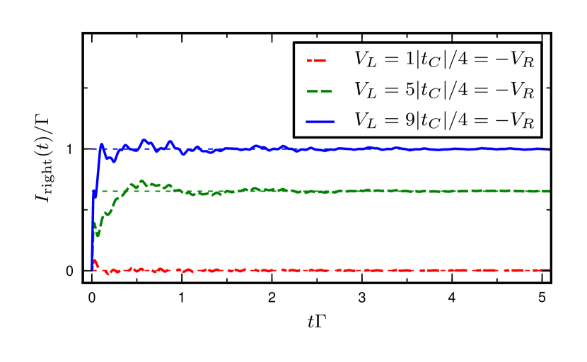
Figure 11: Time-dependent current in units of $\Gamma$ through the right interface with symmetric coupling ($\Gamma=0.1$) and varying bias. (Dotted lines refer to steady-state values.)

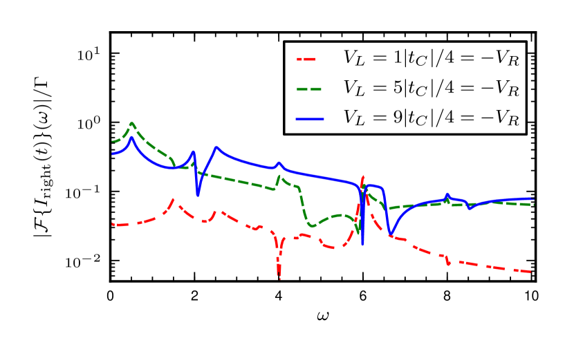
Figure 12: Absolute value of the Fourier transformed right current in units of $\Gamma$. white background text to level the figures. have some more white text. have some more white text.

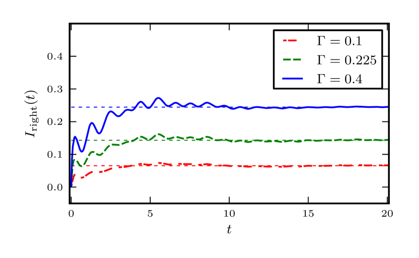
Figure 13: Time-dependent current through the right interface with symmetric coupling (varying strength) and bias $V_{L}=-V_{R}=2.5$. (Dotted lines refer to steady-state values.)

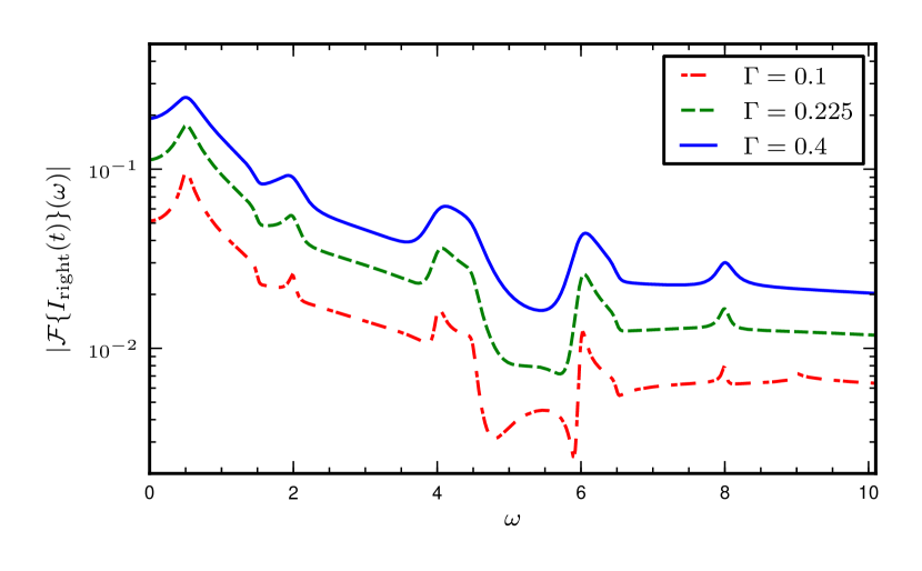
Figure 14: Absolute value of the Fourier transformed right current. white background text to level the figures. have some more white text. have some more white text.

5 Conclusions

In conclusion we solved the Kadanoff–Baym equations for the Green’s function of an open noninteracting system by properly taking into account the initial contacts between the system and the reservoirs. We used the analytic solution for the time-dependent density matrix to derive a time-dependent version of the Landauer–Büttiker formula. As an application we considered a tight-binding benzene-shaped junction and calculated the time-dependent current flowing through it. The advantages of having an explicit solution are that the numerical effort is drastically reduced and that the transient behavior can easily be interpreted in terms of virtual transitions and decay rates. Our time-dependent Landauer–Büttiker formula holds promise for studying the transient behavior of large junctions like, e.g., wide nanoribbons or large-diameter nanotubes, as well as disordered junctions where a large number of simulations is required to perform the average over different configurations.

R.T. wishes to thank Ellen and Artturi Nyyssönen’s foundation for financial support and CSC — the Finnish IT Center for Science — for providing computing resources. We also acknowledge Petri Myöhänen, Anna-Maija Uimonen, Niko Säkkinen and Markku Hyrkäs for productive discussions.

Appendix A Self-energy calculations

The Matsubara self-energy is an antiperiodic function (we are studying fermions) with period given by the inverse temperature $\beta$. For the calculation of the Fourier coefficients we can use the relation: $\mbox{$\mathit{\Sigma}$}^{\text{M}}_{\alpha}({\omega}\pm{\mathrm{i}}\eta)=\mbox{$\mathit{\Sigma}$}_{\alpha}^{\text{R}/\text{A}}({\omega}+\mu)$. Therefore the Matsubara self-energy is simply given by

$$\mbox{$\mathit{\Sigma}$}^{\text{M}}_{\alpha,mn}(\tau,\tau^{\prime}) = \frac{1}{-{\mathrm{i}}\beta}\sum_{q}{\mathrm{e}}^{-{\omega}_{q}(\tau-\tau^{\prime})}\mbox{$\mathit{\Sigma}$}^{\text{M}}_{\alpha,mn}({\omega}_{q})$$ (37)

where

$$\mbox{$\mathit{\Sigma}$}^{\text{M}}_{\alpha,mn}({\omega}_{q})=\left\{\begin{array}[]{ll}-\frac{{\mathrm{i}}}{2}\mbox{$\mathit{\Gamma}$}_{\alpha}&\operatorname{Im}[{\omega}_{q}]>0\\ \\ +\frac{{\mathrm{i}}}{2}\mbox{$\mathit{\Gamma}$}_{\alpha}&\operatorname{Im}[{\omega}_{q}]<0\end{array}\right.$$ (38)

and ${\omega}_{q}=(2q+1)\pi/(-{\mathrm{i}}\beta)$ are the Matsubara frequencies. For the isolated Green’s function of the biased $\alpha$:th reservoir we have

$$g^{\text{R}}_{k\alpha}(t,t_{0}) = -{\mathrm{i}}\theta(t-t_{0}){\mathrm{e}}^{-{\mathrm{i}}(\epsilon_{k\alpha}+V_{\alpha})(t-t_{0})}\ ,$$ (39)

$$g^{\text{M}}_{k\alpha}(\tau,\tau^{\prime}) = \frac{1}{-{\mathrm{i}}\beta}\sum_{q}\frac{{\mathrm{e}}^{-{\omega}_{q}(\tau-\tau^{\prime})}}{{\omega}_{q}-\epsilon_{k\alpha}+\mu}\ .$$ (40)

Without loss of generality we take the time $t_{0}$ at which the bias is switched on to be zero. Then we can write

$$g_{k\alpha}^{\rceil}(t,\tau) = {\mathrm{i}}g^{\text{R}}_{k\alpha}(t,0)g^{\text{M}}_{k\alpha}(0,\tau)={\mathrm{e}}^{-{\mathrm{i}}(\epsilon_{k\alpha}+V_{\alpha})t}g^{\text{M}}_{k\alpha}(0,\tau)\ ,$$ (41)

$$g_{k\alpha}^{\lceil}(\tau,t) = -{\mathrm{i}}g^{\text{M}}_{k\alpha}(\tau,0)g^{\text{A}}_{k\alpha}(0,t)={\mathrm{e}}^{{\mathrm{i}}(\epsilon_{k\alpha}+V_{\alpha})t}g^{\text{M}}_{k\alpha}(\tau,0)\ .$$ (42)

By using Eqs. (41) and (42) we can calculate the right and left embedding self-energies

$$\mbox{$\mathit{\Sigma}$}_{\alpha,mn}^{\rceil}(t,\tau) = \frac{1}{-{\mathrm{i}}\beta}\sum_{q}{\mathrm{e}}^{{\omega}_{q}\tau}\sum_{k}T_{m,k\alpha}\frac{{\mathrm{e}}^{-{\mathrm{i}}(\epsilon_{k\alpha}+V_{\alpha})t}}{{\omega}_{q}-\epsilon_{k\alpha}+\mu}T_{k\alpha,n}$$ (43)

$$= \mbox{$\mathit{\Gamma}$}_{\alpha,mn}\frac{1}{-{\mathrm{i}}\beta}\sum_{q}{\mathrm{e}}^{{\omega}_{q}\tau}{\int\frac{{\mathrm{d}}\omega}{2\pi}}\frac{{\mathrm{e}}^{-{\mathrm{i}}({\omega}+V_{\alpha})t}}{{\omega}_{q}-{\omega}+\mu}\ ,$$

$$\mbox{$\mathit{\Sigma}$}_{\alpha,mn}^{\lceil}(\tau,t) = \frac{1}{-{\mathrm{i}}\beta}\sum_{q}{\mathrm{e}}^{-{\omega}_{q}\tau}\sum_{k}T_{m,k\alpha}\frac{{\mathrm{e}}^{{\mathrm{i}}(\epsilon_{k\alpha}+V_{\alpha})t}}{{\omega}_{q}-\epsilon_{k\alpha}+\mu}T_{k\alpha,n}$$ (44)

$$= \mbox{$\mathit{\Gamma}$}_{\alpha,mn}\frac{1}{-{\mathrm{i}}\beta}\sum_{q}{\mathrm{e}}^{-{\omega}_{q}\tau}{\int\frac{{\mathrm{d}}\omega}{2\pi}}\frac{{\mathrm{e}}^{{\mathrm{i}}({\omega}+V_{\alpha})t}}{{\omega}_{q}-{\omega}+\mu}\ ,$$

where we used $\mbox{$\mathit{\Gamma}$}_{\alpha,mn}=2\pi\sum_{k}T_{mk\alpha}\delta({\omega}-\epsilon_{k\alpha}-V_{\alpha})T_{k\alpha n}$. It only remains to calculate the lesser component. We have

$$g^{<}_{k\alpha}(t,t^{\prime})={\mathrm{i}}f(\epsilon_{k\alpha}-\mu){\mathrm{e}}^{-{\mathrm{i}}(\epsilon_{k\alpha}+V_{\alpha})(t-t^{\prime})}$$ (45)

and therefore

$$\mbox{$\mathit{\Sigma}$}_{\alpha,mn}^{<}(t,t^{\prime}) = \sum_{k}T_{m,k\alpha}{\mathrm{i}}f(\epsilon_{k\alpha}-\mu){\mathrm{e}}^{-{\mathrm{i}}(\epsilon_{k\alpha}+V_{\alpha})(t-t^{\prime})}T_{k\alpha,n}$$ (46)

$$= {\mathrm{i}}\mbox{$\mathit{\Gamma}$}_{\alpha,mn}{\int\frac{{\mathrm{d}}\omega}{2\pi}}f(\omega-\mu){\mathrm{e}}^{-{\mathrm{i}}({\omega}+V_{\alpha})(t-t^{\prime})}\,.$$

Appendix B Green’s function calculations

The Fourier coefficient of the Matsubara Green’s function reads

$$G^{\text{M}}({\omega}_{q}) = \frac{1}{{\omega}_{q}-h-\mbox{$\mathit{\Sigma}$}^{\text{M}}_{\rm em}({\omega}_{q})+\mu}=\begin{cases}\frac{1}{{\omega}_{q}-h+\frac{{\mathrm{i}}}{2}\mbox{$\mathit{\Gamma}$}+\mu}&\operatorname{Im}[{\omega}_{q}]>0\\ \frac{1}{{\omega}_{q}-h-\frac{{\mathrm{i}}}{2}\mbox{$\mathit{\Gamma}$}+\mu}&\operatorname{Im}[{\omega}_{q}]<0\end{cases}$$ (47)

$$= \begin{cases}\frac{1}{{\omega}_{q}-h_{\text{eff}}+\mu}&\operatorname{Im}[{\omega}_{q}]>0\\ \frac{1}{{\omega}_{q}-h_{\text{eff}}^{\dagger}+\mu}&\operatorname{Im}[{\omega}_{q}]<0\ ,\end{cases}$$

where we defined $h_{\text{eff}}=h-\frac{{\mathrm{i}}}{2}\mbox{$\mathit{\Gamma}$}$. The right component of the Green’s function can be derived from the equation of motion

$$\left[{\mathrm{i}}\frac{{\mathrm{d}}}{{\mathrm{d}}t}-h\right]G^{\rceil}(t,\tau)=\int_{0}^{\infty}{\mathrm{d}}\bar{t}\mbox{$\mathit{\Sigma}$}^{\text{R}}_{\rm em}(t,\bar{t})G^{\rceil}(\bar{t},\tau)-{\mathrm{i}}\int_{0}^{\beta}{\mathrm{d}}\bar{\tau}\mbox{$\mathit{\Sigma}$}_{\rm em}^{\rceil}(t,\bar{\tau})G^{\text{M}}(\bar{\tau},\tau)\ .$$ (48)

The insertion of the retarded self-energy from Eq. (20) leads to

$$G^{\rceil}(t,\tau)={\mathrm{e}}^{-{\mathrm{i}}h_{\text{eff}}t}\Big{[}G^{\text{M}}(0,\tau)-\int_{0}^{t}{\mathrm{d}}t^{\prime}{\mathrm{e}}^{{\mathrm{i}}h_{\text{eff}}t^{\prime}}\int_{0}^{\beta}{\mathrm{d}}\bar{\tau}\mbox{$\mathit{\Sigma}$}_{\rm em}^{\rceil}(t^{\prime},\bar{\tau})G^{\text{M}}(\bar{\tau},\tau)\Big{]}\ ,$$ (49)

where we noticed that $G^{\text{M}}(0,\tau)=G^{\rceil}(0,\tau)$.

Finally the retarded Green’s function in Fourier space reads

$$G^{\text{R}}({\omega})=\frac{1}{{\omega}-h-\mbox{$\mathit{\Sigma}$}^{\text{R}}_{\rm em}({\omega})}=\frac{1}{{\omega}-h+\frac{{\mathrm{i}}}{2}\mbox{$\mathit{\Gamma}$}}$$ (50)

and Fourier transforming back in the time domain we recover Eq. (25).

Appendix C The three terms in Eq. (18)

For the first term we use Eqs. (25) and (46) to obtain

$$\left[G^{\text{R}}\cdot\mbox{$\mathit{\Sigma}$}_{\rm em}^{<}\right](t,t) = \int_{0}^{\infty}{\mathrm{d}}\bar{t}\,G^{\text{R}}(t,\bar{t})\mbox{$\mathit{\Sigma}$}_{\rm em}^{<}(\bar{t},t)$$ (51)

$$= {\mathrm{i}}\sum_{\alpha}{\int\frac{{\mathrm{d}}\omega}{2\pi}}f(\omega-\mu)\left[1-{\mathrm{e}}^{{\mathrm{i}}({\omega}+V_{\alpha}-h_{\text{eff}})}\right]G^{\text{R}}({\omega}+V_{\alpha})\mbox{$\mathit{\Gamma}$}_{\alpha}\ .$$

Also the second term is readily calculated by using Eq. (21)

$$\left[G^{<}\cdot\mbox{$\mathit{\Sigma}$}^{\text{A}}_{\rm em}\right](t,t)=\int_{0}^{\infty}{\mathrm{d}}\bar{t}\,G^{<}(t,\bar{t})\mbox{$\mathit{\Sigma}$}^{\text{A}}_{\rm em}(\bar{t},t)=\frac{{\mathrm{i}}}{2}G^{<}(t,t)\mbox{$\mathit{\Gamma}$}\ .$$ (52)

The third term involves somewhat more trickery because of the rather complicated form of the right Green’s function. Inserting the expressions from Eqs. (49) and (44) we get

$$\left[G^{\rceil}\star\mbox{$\mathit{\Sigma}$}_{\rm em}^{\lceil}\right](t,t) = -{\mathrm{i}}\int_{0}^{\beta}{\mathrm{d}}\tau\,G^{\rceil}(t,\tau)\mbox{$\mathit{\Sigma}$}_{\rm em}^{\lceil}(\tau,t)$$

$$= {\mathrm{e}}^{-{\mathrm{i}}h_{\text{eff}}t}\left\{\left[G^{\text{M}}\star\mbox{$\mathit{\Sigma}$}_{\rm em}^{\lceil}\right](0,t)-{\mathrm{i}}\int_{0}^{t}{\mathrm{d}}t^{\prime}{\mathrm{e}}^{{\mathrm{i}}h_{\text{eff}}t^{\prime}}\left[\mbox{$\mathit{\Sigma}$}_{\rm em}^{\rceil}\star G^{\text{M}}\star\mbox{$\mathit{\Sigma}$}_{\rm em}^{\lceil}\right](t^{\prime},t)\right\}.$$

By using $\int_{0}^{\beta}{\mathrm{d}}\tau{\mathrm{e}}^{({\omega}_{q}-{\omega}_{q^{\prime}})\tau}=\beta\delta_{qq^{\prime}}$ for the Matsubara frequencies we may manipulate Eq. (C) further. Inserting Eqs. (43), (44) and (47) we obtain for the double convolution

$$\left[\mbox{$\mathit{\Sigma}$}_{\rm em}^{\rceil}\star G^{\text{M}}\star\mbox{$\mathit{\Sigma}$}_{\rm em}^{\lceil}\right](t^{\prime},t) = -{\mathrm{i}}\int_{0}^{\beta}{\mathrm{d}}\tau(-{\mathrm{i}})\int_{0}^{\beta}{\mathrm{d}}\bar{\tau}\mbox{$\mathit{\Sigma}$}_{\rm em}^{\rceil}(t^{\prime},\bar{\tau})G^{\text{M}}(\bar{\tau},\tau)\mbox{$\mathit{\Sigma}$}_{\rm em}^{\lceil}(\tau,t)$$

$$= {\int\frac{{\mathrm{d}}\omega}{2\pi}}{\int\frac{{\mathrm{d}}\omega^{\prime}}{2\pi}}\sum_{\alpha,\alpha^{\prime}}\mbox{$\mathit{\Gamma}$}_{\alpha}\frac{1}{-{\mathrm{i}}\beta}\sum_{q}\frac{{\mathrm{e}}^{-{\mathrm{i}}({\omega}+V_{\alpha})t^{\prime}}}{{\omega}_{q}-{\omega}+\mu}G^{\text{M}}({\omega}_{q})\frac{{\mathrm{e}}^{{\mathrm{i}}({\omega}^{\prime}+V_{\alpha^{\prime}})t}}{{\omega}_{q}-{\omega}^{\prime}+\mu}\mbox{$\mathit{\Gamma}$}_{\alpha^{\prime}}\ .$$

The integration with respect to ${\omega}$ can be done by closing the contour in lower-half plane (LHP) because of the exponential convergence factor, whereas the integration with respect to ${\omega}^{\prime}$ can be done by closing the contour in the upper-half plane (UHP). However, the corresponding poles are located on different half planes, and this makes the double integral to vanish for every ${\omega}_{q}$. Hence

$$\left[\mbox{$\mathit{\Sigma}$}_{\text{em}}^{\rceil}\star G^{\text{M}}\star\mbox{$\mathit{\Sigma}$}_{\text{em}}^{\lceil}\right](t^{\prime},t)=0\ ,$$ (55)

and in Eq. (C) we are left with

$$\left[G^{\text{M}}\star\mbox{$\mathit{\Sigma}$}_{\text{em}}^{\lceil}\right](0,t) = -{\mathrm{i}}\int_{0}^{\beta}{\mathrm{d}}\tau G^{\text{M}}(0,\tau)\mbox{$\mathit{\Sigma}$}_{\text{em}}^{\lceil}(\tau,t)$$ (56)

$$= {\int\frac{{\mathrm{d}}\omega}{2\pi}}\frac{1}{-{\mathrm{i}}\beta}\sum_{q}\frac{G^{\text{M}}({\omega}_{q}){\mathrm{e}}^{\eta{\omega}_{q}}}{{\omega}_{q}-{\omega}+\mu}\sum_{\alpha}\mbox{$\mathit{\Gamma}$}_{\alpha}{\mathrm{e}}^{{\mathrm{i}}({\omega}+V_{\alpha})t}\ ,$$

where on the last line a convergence factor ${\mathrm{e}}^{\eta{\omega}_{q}}$ was added to account for correct limiting behaviour when $t\to 0$. The sum over Matsubara frequencies can be performed using the Luttinger–Ward trick [13] and yields

$$\frac{1}{-{\mathrm{i}}\beta}\sum_{q}\frac{G^{\text{M}}({\omega}_{q}){\mathrm{e}}^{\eta{\omega}_{q}}}{{\omega}_{q}-{\omega}+\mu} = \int_{\gamma}\frac{{\mathrm{d}}{\omega}^{\prime}}{2\pi}f({\omega}^{\prime}){\mathrm{e}}^{\eta{\omega}^{\prime}}\frac{G^{\text{M}}({\omega}^{\prime})}{{\omega}^{\prime}-{\omega}+\mu}$$ (57)

$$= \int_{-\infty}^{\infty}\frac{{\mathrm{d}}{\omega}^{\prime}}{2\pi}f({\omega}^{\prime})\left[\frac{G^{\text{M}}({\omega}^{\prime}-{\mathrm{i}}\delta)}{{\omega}^{\prime}-{\omega}+\mu-{\mathrm{i}}\delta}-\frac{G^{\text{M}}({\omega}^{\prime}+{\mathrm{i}}\delta)}{{\omega}^{\prime}-{\omega}+\mu+{\mathrm{i}}\delta}\right]\ .$$

By inserting Eq. (57) into Eq. (56) we get

$$\left[G^{\text{M}}\star\mbox{$\mathit{\Sigma}$}_{\rm em}^{\lceil}\right](0,t)={\int\frac{{\mathrm{d}}\omega}{2\pi}}{\int\frac{{\mathrm{d}}\omega^{\prime}}{2\pi}}f({\omega}^{\prime})\left[\frac{G^{\text{M}}({\omega}^{\prime}-{\mathrm{i}}\delta)}{{\omega}^{\prime}-{\omega}+\mu-{\mathrm{i}}\delta}-\frac{G^{\text{M}}({\omega}^{\prime}+{\mathrm{i}}\delta)}{{\omega}^{\prime}-{\omega}+\mu+{\mathrm{i}}\delta}\right]\sum_{\alpha}\mbox{$\mathit{\Gamma}$}_{\alpha}{\mathrm{e}}^{{\mathrm{i}}({\omega}+V_{\alpha})t}\ .$$ (58)

Now the integral over ${\omega}$ can be done by closing the contour in the UHP. The first term in square brackets integrates to zero because of the pole in the LHP. The pole of the second term occurs at ${\omega}={\omega}^{\prime}+\mu+{\mathrm{i}}\delta$, and therefore

$$\left[G^{\text{M}}\star\mbox{$\mathit{\Sigma}$}_{\rm em}^{\lceil}\right](0,t) = {\mathrm{i}}{\int\frac{{\mathrm{d}}\omega^{\prime}}{2\pi}}f({\omega}^{\prime})G^{\text{M}}({\omega}^{\prime}+{\mathrm{i}}\delta)\sum_{\alpha}{\mathrm{e}}^{{\mathrm{i}}({\omega}^{\prime}+\mu+{\mathrm{i}}\delta+V_{\alpha})t}$$

$$\scriptsize\left.\begin{matrix}\delta\to 0^{+}\\ {\omega}^{\prime}={\omega}-\mu\end{matrix}\ \right\}\ \rightarrow\ = {\mathrm{i}}{\int\frac{{\mathrm{d}}\omega}{2\pi}}f(\omega-\mu)\underbrace{G^{\text{M}}({\omega}-\mu)}_{=G^{\text{R}}({\omega})}\sum_{\alpha}\mbox{$\mathit{\Gamma}$}_{\alpha}{\mathrm{e}}^{{\mathrm{i}}({\omega}-\mu+\mu+V_{\alpha})t}$$ (59)

$$= {\mathrm{i}}{\int\frac{{\mathrm{d}}\omega}{2\pi}}f(\omega-\mu)G^{\text{R}}({\omega})\sum_{\alpha}\mbox{$\mathit{\Gamma}$}_{\alpha}{\mathrm{e}}^{{\mathrm{i}}({\omega}+V_{\alpha})}\ .$$

This can be inserted into Eq. (C) to obtain

$$\left[G^{\rceil}\star\mbox{$\mathit{\Sigma}$}_{\rm em}^{\lceil}\right](t,t)={\mathrm{i}}{\int\frac{{\mathrm{d}}\omega}{2\pi}}f(\omega-\mu)\sum_{\alpha}{\mathrm{e}}^{{\mathrm{i}}({\omega}+V_{\alpha}-h_{\text{eff}})t}G^{\text{R}}({\omega})\mbox{$\mathit{\Gamma}$}_{\alpha}\ .$$ (60)

Appendix D Derivation of Eq. (30)

We first state some useful identities for the retarded/advanced Green’s function to be used later:

$$G^{\rm R/A}({\omega}+V_{\alpha})=G^{\rm R/A}({\omega})-V_{\alpha}G^{\rm R/A}({\omega})G^{\rm R/A}({\omega}+V_{\alpha})\ ,$$ (61)

which can be checked directly by using Eq. (50) and its adjoint. From Eq. (61) it follows that

$$V_{\alpha}^{2}G^{\text{R}}({\omega})G^{\text{A}}({\omega})G^{\text{R}}({\omega}+V_{\alpha})G^{\text{A}}({\omega}+V_{\alpha})=\left[G^{\text{R}}({\omega})-G^{\text{R}}({\omega}+V_{\alpha})\right]\left[G^{\text{A}}({\omega})-G^{\text{A}}({\omega}+V_{\alpha})\right]\ .$$ (62)

Taking into account Eq. (61) in Eq. (29) we get

$${\mathrm{i}}\frac{{\mathrm{d}}}{{\mathrm{d}}t}G^{<}(t,t)-h_{\text{eff}}G^{<}(t,t)+G^{<}(t,t)h_{\text{eff}}^{\dagger}$$ (63)

$$= -{\mathrm{i}}{\int\frac{{\mathrm{d}}\omega}{2\pi}}f(\omega-\mu)\sum_{\alpha}\left\{{\mathrm{e}}^{{\mathrm{i}}({\omega}+V_{\alpha}-h_{\text{eff}})t}V_{\alpha}G^{\text{R}}({\omega})G^{\text{R}}({\omega}+V_{\alpha})+G^{\text{R}}({\omega}+V_{\alpha})\right\}\mbox{$\mathit{\Gamma}$}_{\alpha}$$

$$+ {\mathrm{i}}{\int\frac{{\mathrm{d}}\omega}{2\pi}}f(\omega-\mu)\sum_{\alpha}\mbox{$\mathit{\Gamma}$}_{\alpha}\left\{G^{\text{A}}({\omega}+V_{\alpha})G^{\text{A}}({\omega})V_{\alpha}{\mathrm{e}}^{-{\mathrm{i}}({\omega}+V_{\alpha}-h_{\text{eff}}^{\dagger})t}+G^{\text{A}}({\omega}+V_{\alpha})\right\}\ .$$

It is convenient to rewrite the Green’s function as $G^{<}(t,t)={\mathrm{e}}^{-{\mathrm{i}}h_{\text{eff}}t}\tilde{G}^{<}(t,t){\mathrm{e}}^{{\mathrm{i}}h_{\text{eff}}^{\dagger}t}$. In this way the left-hand side of Eq. (63) becomes

$${\mathrm{i}}\frac{{\mathrm{d}}}{{\mathrm{d}}t}\left[{\mathrm{e}}^{-{\mathrm{i}}h_{\text{eff}}t}\tilde{G}^{<}(t,t){\mathrm{e}}^{{\mathrm{i}}h_{\text{eff}}^{\dagger}t}\right]-h_{\text{eff}}{\mathrm{e}}^{-{\mathrm{i}}h_{\text{eff}}t}\tilde{G}^{<}(t,t){\mathrm{e}}^{{\mathrm{i}}h_{\text{eff}}^{\dagger}t}+{\mathrm{e}}^{-{\mathrm{i}}h_{\text{eff}}t}\tilde{G}^{<}(t,t){\mathrm{e}}^{{\mathrm{i}}h_{\text{eff}}^{\dagger}t}h_{\text{eff}}^{\dagger}$$ (64)

$$= {\mathrm{e}}^{-{\mathrm{i}}h_{\text{eff}}t}{\mathrm{i}}\frac{{\mathrm{d}}}{{\mathrm{d}}t}\tilde{G}^{<}(t,t){\mathrm{e}}^{{\mathrm{i}}h_{\text{eff}}^{\dagger}t}\ .$$

Then the right-hand side of Eq. (63) can be multiplied from left by ${\mathrm{e}}^{{\mathrm{i}}h_{\text{eff}}t}$ and from right by ${\mathrm{e}}^{-{\mathrm{i}}h_{\text{eff}}^{\dagger}t}$ to give

$${\mathrm{i}}\frac{{\mathrm{d}}}{{\mathrm{d}}t}\tilde{G}^{<}(t,t) = -{\mathrm{i}}{\int\frac{{\mathrm{d}}\omega}{2\pi}}f(\omega-\mu)\sum_{\alpha}{\mathrm{e}}^{{\mathrm{i}}h_{\text{eff}}t}\left[G^{\text{R}}({\omega}+V_{\alpha})\mbox{$\mathit{\Gamma}$}_{\alpha}-\mbox{$\mathit{\Gamma}$}_{\alpha}G^{\text{A}}({\omega}+V_{\alpha})\right]{\mathrm{e}}^{{\mathrm{i}}h_{\text{eff}}^{\dagger}t}$$ (65)

$$-{\mathrm{i}}{\int\frac{{\mathrm{d}}\omega}{2\pi}}f(\omega-\mu)\sum_{\alpha}V_{\alpha}\left[G^{\text{R}}({\omega})G^{\text{R}}({\omega}+V_{\alpha})\mbox{$\mathit{\Gamma}$}_{\alpha}{\mathrm{e}}^{{\mathrm{i}}({\omega}+V_{\alpha}-h_{\text{eff}}^{\dagger})t}\right.$$

$$\hskip 120.0pt\left.-{\mathrm{e}}^{-{\mathrm{i}}({\omega}+V_{\alpha}-h_{\text{eff}})t}\mbox{$\mathit{\Gamma}$}_{\alpha}G^{\text{A}}({\omega}+V_{\alpha})G^{\text{A}}({\omega})\right]\ .$$

Now we are ready to integrate both sides over $t$ to obtain

$$\tilde{G}^{<}(t,t)-\underbrace{\tilde{G}^{<}(0,0^{+})}_{\mathclap{=G^{<}(0,0^{+})=G^{\text{M}}(0,0^{+})}} = -{\int\frac{{\mathrm{d}}\omega}{2\pi}}f(\omega-\mu)\sum_{\alpha}\int_{0}^{t}{\mathrm{d}}t^{\prime}$$ (66)

$$\times\left\{{\mathrm{e}}^{{\mathrm{i}}h_{\text{eff}}t^{\prime}}\left[G^{\text{R}}({\omega}+V_{\alpha})\mbox{$\mathit{\Gamma}$}_{\alpha}-\mbox{$\mathit{\Gamma}$}_{\alpha}G^{\text{A}}({\omega}+V_{\alpha})\right]{\mathrm{e}}^{-{\mathrm{i}}h_{\text{eff}}^{\dagger}t^{\prime}}\right.$$

$$\hskip 14.22636pt-V_{\alpha}\left[G^{\text{R}}({\omega})G^{\text{R}}({\omega}+V_{\alpha})\mbox{$\mathit{\Gamma}$}_{\alpha}{\mathrm{e}}^{{\mathrm{i}}({\omega}+V_{\alpha}-h_{\text{eff}}^{\dagger})t^{\prime}}\right.$$

$$\left.\left.\hskip 42.67912pt-{\mathrm{e}}^{-{\mathrm{i}}({\omega}+V_{\alpha}-h_{\text{eff}})t^{\prime}}\mbox{$\mathit{\Gamma}$}_{\alpha}G^{\text{A}}({\omega}+V_{\alpha})G^{\text{A}}({\omega})\right]\right\}\ .$$

The integration over $t^{\prime}$ for the second term in Eq (66) can easily be done. For the first term we need the following result: Given two arbitrary matrices $A$ and $B$

$$\int_{0}^{t}{\mathrm{d}}t^{\prime}{\mathrm{e}}^{{\mathrm{i}}At^{\prime}}\left[\frac{1}{x-A}B-B\frac{1}{x-A^{\dagger}}\right]{\mathrm{e}}^{-{\mathrm{i}}A^{\dagger}t^{\prime}}=-{\mathrm{i}}{\mathrm{e}}^{{\mathrm{i}}At^{\prime}}\frac{1}{x-A}B\frac{1}{x-A^{\dagger}}{\mathrm{e}}^{-{\mathrm{i}}A^{\dagger}t^{\prime}}\ ,$$ (67)

which can directly be verified by differentiating the right-hand side with respect to $t^{\prime}$. Applying this result to Eq. (66) we obtain

$$\tilde{G}^{<}(t,t) = {\mathrm{i}}{\int\frac{{\mathrm{d}}\omega}{2\pi}}f(\omega-\mu)\sum_{\alpha}\left\{G^{\text{R}}({\omega})\mbox{$\mathit{\Gamma}$}_{\alpha}G^{\text{A}}({\omega})+{\mathrm{e}}^{{\mathrm{i}}h_{\text{eff}}t}G^{\text{R}}({\omega}+V_{\alpha})\mbox{$\mathit{\Gamma}$}_{\alpha}G^{\text{A}}({\omega}+V_{\alpha}){\mathrm{e}}^{-{\mathrm{i}}h_{\text{eff}}^{\dagger}t}\right.$$ (68)

$$\left.\hskip 85.0pt-G^{\text{R}}({\omega}+V_{\alpha})\mbox{$\mathit{\Gamma}$}_{\alpha}G^{\text{A}}({\omega}+V_{\alpha})\right.$$

$$\left.\hskip 85.0pt+V_{\alpha}G^{\text{R}}({\omega})G^{\text{R}}({\omega}+V_{\alpha})\mbox{$\mathit{\Gamma}$}_{\alpha}G^{\text{A}}({\omega})G^{\text{A}}({\omega}+V_{\alpha}){\mathrm{e}}^{{\mathrm{i}}({\omega}+V_{\alpha}-h_{\text{eff}}^{\dagger})t}\right.$$

$$\left.\hskip 85.0pt-V_{\alpha}G^{\text{R}}({\omega})G^{\text{R}}({\omega}+V_{\alpha})\mbox{$\mathit{\Gamma}$}_{\alpha}G^{\text{A}}({\omega})G^{\text{A}}({\omega}+V_{\alpha})\right.$$

$$\left.\hskip 85.0pt+V_{\alpha}G^{\text{R}}({\omega}+V_{\alpha}){\mathrm{e}}^{-{\mathrm{i}}({\omega}+V_{\alpha}-h_{\text{eff}})t}\mbox{$\mathit{\Gamma}$}_{\alpha}G^{\text{A}}({\omega}+V_{\alpha})G^{\text{A}}({\omega})\right.$$

$$\left.\hskip 85.0pt-V_{\alpha}G^{\text{R}}({\omega}+V_{\alpha})\mbox{$\mathit{\Gamma}$}_{\alpha}G^{\text{A}}({\omega}+V_{\alpha})G^{\text{A}}({\omega})\right\}\ .$$

Then the definition for $\tilde{G}$ can be inserted into the left-hand side, and multiply accordingly with ${\mathrm{e}}^{-{\mathrm{i}}h_{\text{eff}}t}$ from left and with ${\mathrm{e}}^{{\mathrm{i}}h_{\text{eff}}^{\dagger}t}$ from right. Combining terms according to Eqs. (61) and (62) we find Eq. (30).

References

• [1] Landauer R 1957 IBM J. Res. Dev. 1 233
• [2] Büttiker M 1986 Phys. Rev. Lett. 57 1761
• [3] Caroli C, Combescot R, Nozières P and Saint-James D 1971 J. Phys. C 4 916
• [4] Caroli C, Combescot R, Lederer D, Nozières P and Saint-James D 1971 J. Phys. C 4 2598
• [5] Cini M 1980 Phys. Rev. B 22 5887
• [6] Stefanucci G and Almbladh C O 2004 Phys. Rev. B 69 195318
• [7] Mier Y and Wingreen N S 1992 Phys. Rev. Lett. 68 2512
• [8] Jauho A P, Wingreen N S and Mier Y 1994 Phys. Rev. B. 50 5528
• [9] Pastawski H M 1992 Phys. Rev. B. 46 4053
• [10] Perfetto E, Stefanucci G and Cini M 2008 Phys. Rev. B 78 155301
• [11] Myöhänen P, Stan A, Stefanucci G and van Leeuwen R 2009 Phys. Rev. B 80 115107
• [12] Stefanucci G and van Leeuwen R 2013 Nonequilibrium Many-Body Theory of Quantum systems: A Modern Introduction (Cambridge University Press)
• [13] Luttinger J M and Ward J C 1960 Phys. Rev. 118 1417