Seeing the orbital ordering in Iron-based superconductors with magnetic anisotropy

Abstract

The orbital fluctuation of the conduction electrons in the Iron-based superconductors is found to contribute significantly to the magnetic response of the system. With the use of a realistic five-band model and group theoretical analysis, we have determined the orbital magnetic susceptibility in such a multi-orbital system. At $n=6.1$, the in-plane orbital magnetic susceptibility is predicted to be about 10$\mu_{\mathrm{B}}^{2}/\mathrm{eV}$, which is more than $2/3$ of the observed total susceptibility around 200 K in 122 systems(of about 14$\mu_{\mathrm{B}}^{2}/\mathrm{eV}$ or $4.5\times 10^{-4}\mathrm{erg}/\mathrm{G}^{2}\mathrm{mol}_{\mathrm{AS}}$Klingeler ). We find the in-plane orbital magnetic response is sensitive to the breaking of the tetragonal symmetry in the orbital space. In particular, when the observed band splitting(between the $3d_{xz}$ and the $3d_{yz}$-dominated band) is used to estimate the strength of the symmetry breaking perturbationShen , a 4.5% modulation in the in-plane orbital magnetic susceptibility can be produced, making the latter a useful probe of the orbital ordering in such a multi-orbital system. As a by product, the theory also explains the large anisotropy between the in-plane and the out-of-plane magnetic response observed universally in susceptibility and NMR measurements.

An unresolved issue in the study of the Iron-based superconductors is the role of their multi-orbital nature. In most other superconductors, the orbital degree of freedom is quenched at low energy in the crystal field environment. However, both LDA calculation and ARPES measurementFeng ; Shen ; Shimojima indicate that in the Iron-based superconductors all the five Fe $3d$ orbital play essential role in forming the low energy degree of freedom around the Fermi surface. Many novel properties of the Iron-based superconductors, especially those in the name of electronic nematicityChuang ; ChuPRB ; Chu1 ; Chu2 ; Kasahara , have been argued to be related to the orbital ordering in these systemsKu ; Lv1 ; Singh ; Lv2 ; Nevidomskyy . Most recently, a two-fold modulation of the magnetic susceptibility in the Fe-Fe plane is found to develop around a temperature that is significantly higher than the structural phase transition pointKasahara . However, it is still a mystery how the observed electronic nematicity is related to the orbital ordering of the system.

Another puzzle about the Iron-based superconductors is the strong anisotropy in their magnetic response observed universally in susceptibility and Knight shift measurementsChenCa ; ChenBa ; CanfieldSr ; Zheng . The susceptibility in the Fe-Fe plane is found to be significantly larger than that perpendicular to it. This is very unusual, since the magnetic response of a transition metal is usually attributed to the spin of its valence electron and is essentially isotropic. The orbital magnetic response, on the other hand, is usually quenched as a result of the crystal field effect. However, since the crystal field splitting in the Iron-based superconductors is very small and all the five $3d$ orbital are involved in the low energy physicsFeng ; Shen ; Shimojima , the orbital angular momentum of the conduction electron can contribute to the magnetic response of these systems. Such a contribution is intrinsically anisotropic and depends on the electronic structure of the system, especially on the symmetry breaking in the orbital space.

The purpose of this paper is to evaluate orbital magnetic response of the Iron-based superconductors from a realistic model and to explore the relation between orbital ordering and the electronic nematicity observed in recent torque magnetometry measurementKasahara . We find the orbital magnetic susceptibility in these multi-orbital systems is comparable in magnitude with the measured total magnetic susceptibility. More specifically, the in-plane orbital magnetic susceptibility is predicted to be about 10$\mu_{\mathrm{B}}^{2}/\mathrm{eV}$, which accounts for more than $2/3$ of the observed susceptibility at 200 K in 122 systemsKlingeler ; ChenCa ; ChenBa ; CanfieldSr . Furthermore, the in-plane orbital magnetic response is found to be sensitive to the breaking of the tetragonal symmetry in the orbital space, making it a useful probe of orbital ordering in these multi-orbital systems. As a by product, the observed strong anisotropy between the in-plane and out-of-plane magnetic susceptibility also find a natural explanation from our calculation.

The Iron-based superconductors have a very complicated band structure. In this study, we adopt the five-band tight-binding model derived from fitting the LDA band structureKuroki of the LaFeAsO system. Following the notations of Ref.Kuroki, , the band model reads,

$$H_{kin}=\sum_{i,j}\sum_{\nu,\nu^{\prime},\sigma}[t_{i,j}^{\nu,\nu^{\prime}}c_{i,\nu,\sigma}^{\dagger}c_{j,\nu^{\prime},\sigma}+h.c.]+\sum_{i,\nu,\sigma}\varepsilon_{\nu}n_{i,\nu,\sigma},$$

(1)

where $\nu,\nu^{\prime}=1,..,5$ is the index for the five maximally localized Wannier functions(MLWFs) on the Fe site, namely, $|1\rangle=|3d_{3Z^{2}-R^{2}}\rangle$, $|2\rangle=|3d_{XZ}\rangle$, $|3\rangle=|3d_{YZ}\rangle$, $|4\rangle=|3d_{X^{2}-Y^{2}}\rangle$ and $|5\rangle=|3d_{XY}\rangle$. $t_{i,j}^{\nu,\nu^{\prime}}$ denotes the hopping integral between the $\nu$-th and $\nu^{\prime}$-th orbital at site $i$ and site $j$. Here an unfolded scheme is adopted as in Ref.Kuroki, . The $X$ and $Y$-axis for the Wannier functions, which are in the Fe-As bond direction, are rotated by 45 degree from the $x$ and $y$-axis of the Fe-Fe square lattice(see Fig.1). $\varepsilon_{\nu}$ is the on-site energy of the $\nu$-th orbital. The hopping integral is truncated at the fifth neighbor and the values of the model parameters can be found in Ref.Kuroki, .

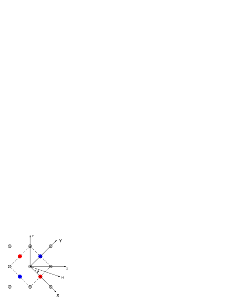
Figure 1: The square lattice of the Fe ions (shown as gray dots) and the local coordinate system for the atomic orbital. The red and blue dots denote the As ions above and below the Fe-Fe plane. $\phi$ is the angle between the $X$-axis and the direction in which magnetic susceptibility is measured. In the tetragonal phase, the point group symmetry around the Fe ion is $D_{2d}$, which is broken down to $D_{2}$ in the orthogonal phase.

The interaction of electron has the following general form

$$H_{int} =U\sum_{i,\nu,\sigma}n_{i,\nu,\sigma}n_{i,\nu,\overline{\sigma}}+(U^{\prime}-J)\sum_{i,\nu^{\prime}\neq\nu,\sigma}n_{i,\nu,\sigma}n_{i,\nu^{\prime},\sigma}$$ (2)

$$+U^{\prime} \sum_{i,\nu^{\prime}\neq\nu,\sigma}n_{i,\nu,\sigma}n_{i,\nu^{\prime},\overline{\sigma}}-J\sum_{i,\nu^{\prime}\neq\nu,\sigma}c^{\dagger}_{i,\nu,\sigma}c_{i,\nu,\overline{\sigma}}c^{\dagger}_{i,\nu^{\prime},\overline{\sigma}}c_{i,\nu^{\prime},\sigma}$$

$$-J \sum_{i,\nu^{\prime}\neq\nu,\sigma}c^{\dagger}_{i,\nu,\sigma}c^{\dagger}_{i,\nu,\overline{\sigma}}c_{i,\nu^{\prime},\sigma}c_{i,\nu^{\prime},\overline{\sigma}}.$$

Here we have included the intra- and inter-orbital Coulomb repulsion, the Hund’s rule coupling and the pair hopping term and have assumed that $U^{\prime}=U-2J$. $n_{i}=\sum_{\nu,\sigma}n_{i,\nu,\sigma}=\sum_{\nu,\sigma}c^{\dagger}_{i,\nu,\sigma}c_{i,\nu,\sigma}$ is the number density operator of the electron and $\overline{\sigma}=-\sigma$.

Since the five Fe $3d$ orbital $|\nu\rangle$ are all real functions, they can not carry current and thus their orbital angular momentum are quenched in the static limit. However, since the orbital content varies on the Fermi surface, fluctuation in the orbital character and orbital angular momentum survives in the low energy limit and can contribute to the magnetic response of the system. In the following we will calculate such a magnetic response in the RPA scheme.

The orbital magnetic susceptibility is defined through the correlation function of the orbital magnetic moment in the following way

$$\chi^{\alpha}_{L}({\mathbf{q}},\tau)=-\langle T_{\tau}\hat{L}^{\alpha}({\mathbf{q}},\tau)\hat{L}^{\alpha}(-{\mathbf{q}},0)\rangle,$$ (3)

in which $\hat{L}^{\alpha}({\mathbf{q}},\tau)$ denotes the Fourier component of the orbital magnetic moment density in the $\alpha$ direction and $\alpha=X,Y,Z$. Here we use $\mu_{B}^{2}$ as the unit of susceptibility. The operator for the orbital magnetic moment on a given site is defined as $\hat{L}^{\alpha}=\sum_{\nu,\nu^{\prime},\sigma}c^{\dagger}_{\nu,\sigma}l^{\alpha}_{\nu,\nu^{\prime}}c_{\nu^{\prime},\sigma}$, where $l^{\alpha}_{\nu,\nu^{\prime}}$ is the matrix element of the orbital magnetic moment in the basis spanned by the five MLWFs.

The matrix element $l^{\alpha}_{\nu,\nu^{\prime}}$ can be determined in principle from a first principle calculation. Here we will be satisfied with the result of a semi-quantitative analysis, for which much simplification can be achieved when symmetry arguments are adopted. In the following, we will illustrate the steps for $l^{Z}_{\nu,\nu^{\prime}}$. First, since $\hat{L}^{Z}$ is time reversal odd and the five $3d$ orbital are all real, $l^{Z}_{\nu,\nu^{\prime}}$ must be purely imaginary. Second, since $\hat{L}^{Z}$ is odd under the action of the three generators of the $D_{2d}$ point group around each Fe ion, namely $R_{x}(\pi)$, $\sigma_{X}$ and $\sigma_{Y}$group , while the five $3d$ orbital transform as

$$R_{x}(\pi):\left(\begin{array}[]{c}|1\rangle\\ |2\rangle\\ |3\rangle\\ |4\rangle\\ |5\rangle\\ \end{array}\right)\rightarrow\left(\begin{array}[]{c}|1\rangle\\ -|3\rangle\\ -|2\rangle\\ -|4\rangle\\ |5\rangle\\ \end{array}\right)$$ (14)

$$\sigma_{X}:\left(\begin{array}[]{c}|1\rangle\\ |2\rangle\\ |3\rangle\\ |4\rangle\\ |5\rangle\\ \end{array}\right)\rightarrow\left(\begin{array}[]{c}|1\rangle\\ -|2\rangle\\ |3\rangle\\ |4\rangle\\ -|5\rangle\\ \end{array}\right)$$ (25)

and

$$\sigma_{Y}:\left(\begin{array}[]{c}|1\rangle\\ |2\rangle\\ |3\rangle\\ |4\rangle\\ |5\rangle\\ \end{array}\right)\rightarrow\left(\begin{array}[]{c}|1\rangle\\ |2\rangle\\ -|3\rangle\\ |4\rangle\\ -|5\rangle\\ \end{array}\right),$$ (36)

the only none-zero matrix elements are $l^{Z}_{2,3}=-l^{Z}_{3,2}$ and $l^{Z}_{4,5}=-l^{Z}_{5,4}$. Thus $\hat{L}^{Z}$ can be generally written as

$$\hat{L}^{Z}=i\sum_{\sigma}[\gamma_{1}c^{\dagger}_{2,\sigma}c_{3,\sigma}+\gamma_{2}c^{\dagger}_{4,\sigma}c_{5,\sigma}]+h.c.,$$

in which $\gamma_{1}$ and $\gamma_{2}$ are two real numbers. Following the same line of reasoning one find that

$$\hat{L}^{X} =i \sum_{\sigma}[\gamma_{3}c^{\dagger}_{1,\sigma}c_{3,\sigma}+\gamma_{4}c^{\dagger}_{2,\sigma}c_{5,\sigma}+\gamma_{5}c^{\dagger}_{3,\sigma}c_{4,\sigma}]+h.c.$$

$$\hat{L}^{Y} =-i \sum_{\sigma}[\gamma_{3}c^{\dagger}_{1,\sigma}c_{2,\sigma}+\gamma_{4}c^{\dagger}_{3,\sigma}c_{5,\sigma}-\gamma_{5}c^{\dagger}_{2,\sigma}c_{4,\sigma}]+h.c.,$$

with the three real coefficients $\gamma_{3,4,5}$ left undetermined.

To have an estimate of the values of the five coefficients $\gamma_{1,..,5}$, we approximate the five MLWFs $|\nu\rangle$, $\nu=1,..,5$, with the five Fe $3d$ orbital in the atomic limit. These atomic orbital are related to the spherical harmonics of $l=2$ in the following ways(apart from the radial part of the wave function which is not used in determining the matrix element of $\hat{L}^{\alpha}$)

$$|1\rangle = |2,0\rangle$$

$$|2\rangle = \frac{1}{\sqrt{2}}\left(|2,-1\rangle-|2,1\rangle\right)$$

$$|3\rangle = \frac{i}{\sqrt{2}}\left(|2,-1\rangle+|2,1\rangle\right)$$

$$|4\rangle = \frac{1}{\sqrt{2}}\left(|2,-2\rangle+|2,2\rangle\right)$$

$$|5\rangle = \frac{i}{\sqrt{2}}\left(|2,-2\rangle-|2,2\rangle\right),$$

where $|2,m\rangle\propto Y^{m}_{2}$ are the spherical harmonics of $l=2$. Since $\langle 2,m^{\prime}|\hat{L}^{Z}|2,m\rangle=m\delta_{m,m^{\prime}}$ and $\langle 2,m|\hat{L}^{+}|2,m^{\prime}\rangle=\sqrt{6-m^{\prime}(m^{\prime}+1)}\delta_{m,m^{\prime}+1}$(here $\hat{L}^{+}=\hat{L}^{X}+i\hat{L}^{Y}$), we have

$$\gamma_{1} =- \gamma_{4}=\gamma_{5}=-1$$

$$\gamma_{2} = -2$$

$$\gamma_{3} = \sqrt{3}.$$

We will use these values in the following calculation.

The bare orbital magnetic susceptibility is readily obtained as

$$\chi^{0,\alpha}_{L}(T) = \lim_{{\mathbf{q}}\rightarrow 0}\frac{2}{N}{\sum_{\mathbf{k},m,m^{\prime}}}\frac{f(\xi_{\mathbf{k+q},m^{\prime}})-f(\xi_{{\mathbf{k}},m})}{\xi_{{\mathbf{k}},m}-\xi_{\mathbf{k+q},m^{\prime}}}\left|L^{\alpha}_{{\mathbf{k}},m,m^{\prime}}\right|^{2}.$$

Here $\xi_{{\mathbf{k}},m}=\epsilon_{{\mathbf{k}},m}-\mu$ is the band energy of the $m$-th band($m=1,...,5$) and $\mu$ is the chemical potential. $L^{\alpha}_{{\mathbf{k}},m,m^{\prime}}=\sum_{\nu,\nu^{\prime}}l^{\alpha}_{\nu,\nu^{\prime}}u^{*}_{{\mathbf{k}},\nu,m}u_{{\mathbf{k}},\nu^{\prime},m^{\prime}}$ and $u_{{\mathbf{k}},\nu,m}$ is the $m$-th eigenvector of the band Hamiltonian at momentum ${\mathbf{k}}$. As a comparison, the Pauli spin susceptibility is given by

$$\chi^{0,\alpha}_{S}(T) = \lim_{{\mathbf{q}}\rightarrow 0}\frac{2}{N}\sum_{{\mathbf{k}},m}\left[\frac{f(\xi_{\mathbf{k+q},m})-f(\xi_{{\mathbf{k}},m})}{\xi_{{\mathbf{k}},m}-\xi_{\mathbf{k+q},m}}\right].$$

Unlike the orbital magnetic susceptibility, the Pauli spin susceptibility has contribution only from intra-band process. Thus at low temperature the spin susceptibility is solely determined by the electronic state around the Fermi surface, while the orbital magnetic susceptibility depends on electronic states both on and far away from the Fermi energy. As a result, both the temperature and the doping dependence of the orbital magnetic response should be much weaker than that of the spin magnetic response.

Now we consider the RPA correction of the orbital magnetic susceptibility. The orbital magnetic excitation of the system has the general form of $\hat{O}^{\nu\nu^{\prime}}=i\sum_{\sigma}(c^{\dagger}_{\nu,\sigma}c_{\nu^{\prime},\sigma}-c^{\dagger}_{\nu^{\prime},\sigma}c_{\nu,\sigma})$. Without losing generality, we assume $\nu^{\prime}>\nu$. There are in total 10 such excitations and all of them are time reversal odd and spin singlet. The correlation function between these excitations can be defined in the following way

$$\chi^{\nu\nu^{\prime},\upsilon\upsilon^{\prime}}_{O}({\mathbf{q}},\tau)=-\langle T_{\tau}\hat{O}^{\nu\nu^{\prime}}({\mathbf{q}},\tau)\hat{O}^{\upsilon\upsilon^{\prime}}(-{\mathbf{q}},0)\rangle,$$

and the corresponding bare susceptibility in the static limit $\chi^{0,\nu\nu^{\prime},\upsilon\upsilon^{\prime}}_{O}(T)$ is given by an expression similar to Eq.(LABEL:eqn6), except that the matrix element $|L^{\alpha}_{{\mathbf{k}},m,m^{\prime}}|^{2}$ should be replaced by

$$O^{\nu\nu^{\prime},\upsilon\upsilon^{\prime}}_{{\mathbf{k}},m,m^{\prime}} = (u^{*}_{{\mathbf{k}},\nu^{\prime},m^{\prime}}u_{{\mathbf{k}},\nu,m}-u^{*}_{{\mathbf{k}},\nu,m^{\prime}}u_{{\mathbf{k}},\nu^{\prime},m})$$

$$\times (u^{*}_{{\mathbf{k}},\upsilon,m}u_{{\mathbf{k}},\upsilon^{\prime},m^{\prime}}-u^{*}_{{\mathbf{k}},\upsilon^{\prime},m}u_{{\mathbf{k}},\upsilon,m^{\prime}}).$$

The RPA correction of $\chi^{\nu\nu^{\prime},\upsilon\upsilon^{\prime}}_{O}$ is contributed by the inter-orbital Coulomb repulsion, the Hund’s rule coupling and the pair hopping term. The RPA kernel is extremely simple and is given by $V_{\nu\nu^{\prime},\upsilon\upsilon^{\prime}}=\frac{(U^{\prime}-J)}{4}\delta_{\nu\nu^{\prime},\upsilon\upsilon^{\prime}}$(see Supplementary material A). The RPA corrected susceptibility can be written formally as

$$\chi_{O}=\frac{\chi^{0}_{O}}{1-V\chi^{0}_{O}},$$

in which $\chi_{O}$, $\chi^{0}_{O}$ and $V$ are all to be understood as $10\times 10$ matrix(we note while $V$ is a diagonal matrix in the space of $\hat{O}^{\nu,\nu^{\prime}}$, $\chi^{0}_{O}$ is not). The orbital magnetic susceptibility can be obtained from the combinations of the matrix element of $\chi_{O}$. For example,

$$\chi^{Z}_{L}=\chi^{23,23}_{O}+4(\chi^{45,45}_{O}+\chi^{23,45}_{O}).$$

The orbital magnetic susceptibility in other direction can be obtained in a similar way.

The observation of the two-fold modulation in the in-plane magnetic susceptibility indicates that the tetragonal symmetry of the system is broken down to orthogonal. This can happen either through orbital ordering, or through nematicity in spin correlationXu ; Chubukov1 . Here we assume it happens through orbital ordering, since the orbital magnetic response is much more sensitive to it than to spin nematicity. The form of the symmetry breaking perturbation in the orthogonal phase can be largely determined by group theoretical arguments. Among the five $3d$ orbital, the $3d_{3Z^{2}-R^{2}}$, $3d_{XY}$ and $3d_{X^{2}-Y^{2}}$ orbital each form a one dimensional representation of the $D_{2d}$ point group. The $3d_{XZ}$ and $3d_{YZ}$ orbital form a two-dimensional representation which becomes reducible when the symmetry is lowered to orthogonal. We thus focus on symmetry breaking terms in the space spanned by the $3d_{XZ}$ and $3d_{YZ}$ orbital. A group theoretical analysis then shows that up to nearest neighboring hopping terms, the only allowable symmetry breaking perturbation in the orthogonal phase takes the form (see Supplementary information B)

$$\Delta H = \eta_{1}\sum_{i,\sigma}(c^{\dagger}_{i,2,\sigma}c_{i,3,\sigma}+c^{\dagger}_{i,3,\sigma}c_{i,2,\sigma})$$ (38)

$$+ \eta_{2}\sum_{i,\delta,\sigma}\mathrm{d}_{\delta}(c^{\dagger}_{i,2,\sigma}c_{i+\delta,2,\sigma}+c^{\dagger}_{i,3,\sigma}c_{i+\delta,3,\sigma})$$

$$+ \eta_{3}\sum_{i,\delta,\sigma}(c^{\dagger}_{i,2,\sigma}c_{i+\delta,3,\sigma}+c^{\dagger}_{i,3,\sigma}c_{i+\delta,2,\sigma}),$$

in which $\delta=\pm x,\pm y$ is the vector between nearest neighboring Fe sites. $\mathrm{d}_{\delta}$ is the d-wave form factor and $\mathrm{d}_{\pm x}=1$, $\mathrm{d}_{\pm y}=-1$. Here, $\eta_{1}$ is the strength of the on-site symmetry breaking perturbation. $\eta_{2}$ and $\eta_{3}$ are the strengths of the d-wave intra-orbital and s-wave inter-orbital hopping terms between nearest neighboring Fe sites. From ARPES measurementShen , it is found that the splitting between the $3d_{xz}$ and the $3d_{yz}$-dominated band is zero at the $\Gamma$ point and maximizes at the X and Y point. Among the three perturbations in Eq.(38), only the d-wave intra-orbital hopping term is consistent with such a momentum dependence. For example, both the $\eta_{1}$ or $\eta_{3}$-type perturbation would result in an nonzero band splitting at the $\Gamma$ point, which is not observed. Furthermore, the $\eta_{3}$-type perturbation has no effect at the X and Y point, where the observed band splitting reaches its maximum. We thus set $\eta_{1}=\eta_{3}=0$. This leaves us $\eta_{2}$ as the only undetermined parameter.

We are now at the position to present the numerical results. Our calculation is done at a fixed band filling of $n=6.1$. The chemical potential is determined by solving the mean field particle number equation at each temperature. We have set $U=1.2$eV, $J=0.15$eV, as is chosen in Ref.Kuroki, . To estimate the value of $\eta_{2}$ from the observed band splitting, we note that the band width of the Iron-based superconductors is significantly smaller than the prediction of band structure calculation. We thus fit the relative rather than the absolute magnitude of the band splitting. According to ARPES measurement, the maximal band splitting between the $3d_{yz}$ and $3d_{xz}$-dominated band is about one half of the dispersion of the $3d_{yz}$-dominated band between the $\Gamma$ and X pointShen . To fit such a splitting, we set $\eta_{2}=30$ meV. The calculated band dispersion along the $\Gamma-\mathrm{X}$ and $\Gamma-\mathrm{Y}$ direction is shown in Fig.2, which looks very similar to the experimental resultShen . The temperature dependence of $\eta_{2}$ is modeled by the mean field form of $\eta_{2}(T)=\eta_{2}(0)\sqrt{1-(T/T_{c})^{2}}$, in which $T_{c}$ is to be understood as the mean field critical temperature of orbital ordering. We set $T_{c}=150$K in our calculationKasahara .

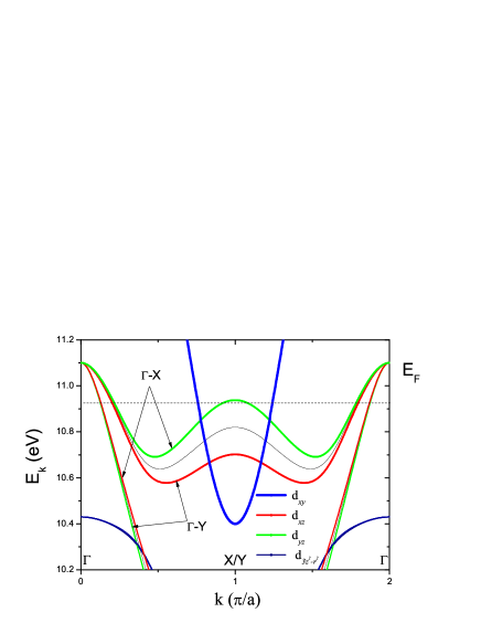
Figure 2: Overlay of the band dispersion along the $\Gamma-\mathrm{X}$ and $\Gamma-\mathrm{Y}$ direction in the orthogonal phase. The orbital character is indicated by the color of the lines and the dispersion in the tetragonal phase is plotted in thin lines for reference. In the calculation we have set $\eta_{2}=30$ meV. The dashed line indicates the Fermi level at $n=6.1$.

In the tetragonal phase, the orbital magnetic susceptibility is found to be isotropic in the Fe-Fe plane and is almost temperature and doping independent for $6.0\leq n\leq 6.2$(see Supplementary material C). This is reasonable since the orbital magnetic response is contributed by the whole band, rather than the electronic state near the Fermi level only. At $n=6.1$, the bare orbital magnetic susceptibility in the Fe-Fe plane is found to be about 7.3$\mu_{\mathrm{B}}^{2}/\mathrm{eV}$, which is enhanced to 10$\mu_{\mathrm{B}}^{2}/\mathrm{eV}$ after RPA correction. This is already comparable to the observed total in-plane magnetic susceptibility at 200K in 122 systems, which is about $4.5\times 10^{-4}\mathrm{erg}/\mathrm{G}^{2}\mathrm{mol}_{\mathrm{AS}}$ (or 14$\mu_{\mathrm{B}}^{2}/\mathrm{eV}$)Klingeler . As a comparison, the bare Pauli spin susceptibility is only about 2$\mu_{\mathrm{B}}^{2}/\mathrm{eV}$.

When a symmetry breaking perturbation of the $\eta_{2}$-type is turned on, a two-fold modulation shows up in the in-plane orbital magnetic susceptibility. The angular dependence of the in-plane susceptibility at $T=T_{c}/5$ is shown in Fig.3a. Here $\phi$ denotes the angle between the $X$-axis and the direction in which the magnetic susceptibility is measured. The relative strength of the modulation is about 2.6% before RPA correction and is enhanced to 4.5% after RPA correction. The principle axes of the modulation are along the direction of the nearest Fe-Fe bond, which is just what we should expect from our model construction. The temperature dependence of the susceptibility in the principle axes are shown in Fig.3b. These predictions are in good agreement with the result of the recent torque magnetometry measurementKasahara . Thus the magnetic anisotropy provide a realistic probe of the orbital ordering in the Iron-based superconductors.

A robust prediction of our theory is the strong anisotropy between the in-plane and the out-of-plane orbital magnetic susceptibility. At $n=6.1$, the bare orbital magnetic susceptibility in $Z$ direction is found to be about 3.8$\mu_{\mathrm{B}}^{2}/\mathrm{eV}$, which is enhanced to 4.5$\mu_{\mathrm{B}}^{2}/eV$ after RPA correction. This is only about the half of the value of the in-plane orbital magnetic susceptibility. We find the ratio between the in-plane and out-of-plane orbital magnetic susceptibility is also almost temperature and doping independent for $6.0\leq n\leq 6.2$ and is always close to 2. According to experiments, both the in-plane and the out-of-plane magnetic susceptibility exhibit linear temperature dependence with almost the same slope. However, the intercept of the in-plane magnetic susceptibility is always much larger than that of the out-of-plane magnetic susceptibilityChenCa ; ChenBa ; CanfieldSr ; Zheng . This behavior can be easily understood if we decompose the measured magnetic susceptibility into an isotropic component that is linearly temperature dependent and a temperature independent component that is anisotropic, or,

$$\chi^{\alpha}(T)=\chi^{\alpha}_{L}+\chi_{S}(T).$$ (39)

It is then quite natural to associate the anisotropic component $\chi^{\alpha}_{L}$ with the orbital magnetic response, which is essentially temperature independent. The isotropic component $\chi_{S}(T)$ should then be attributed to the spin magnetic response, whose linear temperature dependence is still an unresolved issue in the field.GMZhang ; SPKou ; Chubukov2

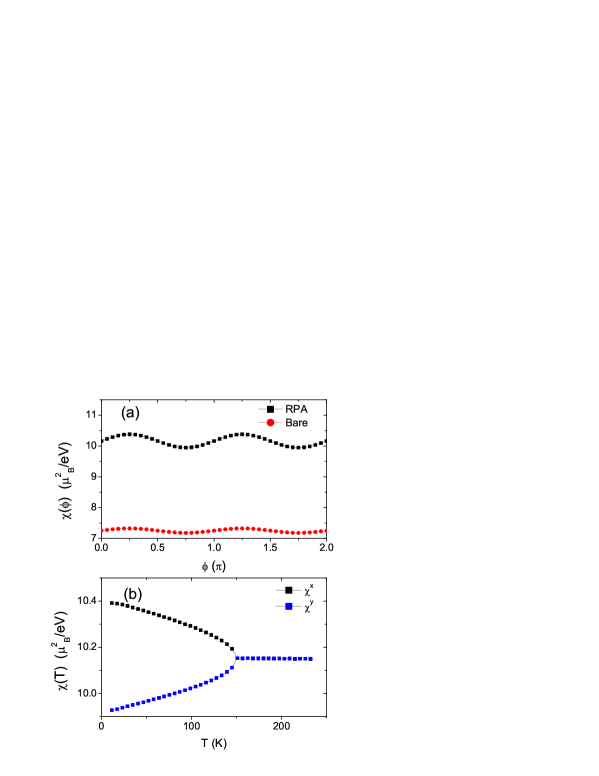
Figure 3: (a)The in-plane modulation of the orbital magnetic susceptibility before and after RPA correction. (b) The temperature dependence of the RPA-corrected orbital magnetic susceptibility along the two principle axes of the orthogonal phase.

In our calculation, we have used a five-band model derived from the band structure of the LaFeAsO system. However, the best known susceptibility data on single crystalline sample are all taken from the 122 system. It is thus better to perform the calculation with a material-specific band structure for the 122 systems. While this is an interesting possibility and should be pursued in the future, we note that the basic structure of the bands in both the 1111 and the 122 systems are quite similar. Since the orbital magnetic response is contributed by the whole band rather than the electronic state near the Fermi level only, we expect the 1111 and 122 system to exhibit similar orbital magnetic response. Another way to improve our calculation is to use the matrix element of $\hat{L}^{\alpha}$ calculated from first principle code, rather than approximating them with those in the basis spanned by the atomic orbital. However, since the form the matrix element is largely determined by symmetry, we do not expect such more advanced calculation to change the conclusion of this paper in a qualitative way. Indeed, we find that our results are not sensitive to the small variation of the parameters $\gamma_{1,.,5}$.

In summary, we have shown that the orbital angular momentum of the conduction electrons in the Iron-based superconductors contributes significantly to the magnetic response of the system. In particular, the theory predicts that the orbital magnetic susceptibility accounts for more than $2/3$ of the observed magnetic susceptibility at 200 K in 122 systems. We show that the orbital magnetic response is sensitive to symmetry breaking in the orbital space, which makes it a useful probe of the orbital ordering in these multi-orbital systems. A large and temperature independent anisotropy between the in-plane and the out-of plane susceptibility is predicted, which provides a natural understanding on the behavior of the magnetic response of these systems.

Yuehua Su is support by NSFC Grant No. 10974167 and Tao Li is supported by NSFC Grant No. 10774187, No. 11034012 and National Basic Research Program of China No. 2010CB923004. We are grateful to K. Kuroki for clarifying the phase convention used in Ref.Kuroki, .

I Supplementary materials

I.1 The form of the RPA kernel for orbital magnetic excitations

The ten orbital magnetic excitation of the form $\hat{O}^{\nu\nu^{\prime}}=i\sum_{\sigma}(c^{\dagger}_{\nu,\sigma}c_{\nu^{\prime},\sigma}-c^{\dagger}_{\nu^{\prime},\sigma}c_{\nu,\sigma})$ are all time reversal odd and spin rotational invariant. In the absence of time reversal symmetry breaking they form a subspace within the space of all orbital excitations. It is thus sufficient to restrict our consideration in this subspace.

The RPA correction to the orbital magnetic response is contributed by the inter-orbital Coulomb term, the Hund’s rule coupling term and the pair hopping term. For example, the inter-orbital Coulomb term has the following mean field decoupling($\nu^{\prime}>\nu$),

$$U^{\prime}n_{i,\nu,\sigma}n_{\i,\nu^{\prime},\sigma}\sim- U^{\prime} \langle c^{\dagger}_{i,\nu,\sigma}c_{i,\nu^{\prime},\sigma}\rangle c^{\dagger}_{i,\nu^{\prime},\sigma}c_{i,\nu,\sigma}$$

$$- U^{\prime} \langle c^{\dagger}_{i,\nu^{\prime},\sigma}c_{i,\nu,\sigma}\rangle c^{\dagger}_{i,\nu,\sigma}c_{i,\nu^{\prime},\sigma}$$

$$+ U^{\prime} \langle c^{\dagger}_{i,\nu,\sigma}c_{i,\nu^{\prime},\sigma}\rangle\langle c^{\dagger}_{i,\nu^{\prime},\sigma}c_{i,\nu,\sigma}\rangle.$$

When expressed in terms of $\hat{O}^{\nu,\nu^{\prime}}$, we have

$$U^{\prime}\sum_{\sigma}n_{i,\nu,\sigma}n_{\i,\nu^{\prime},\sigma}\sim-\frac{U^{\prime}}{4}\langle\hat{O}^{\nu,\nu^{\prime}}\rangle\hat{O}^{\nu,\nu^{\prime}}+\frac{U^{\prime}}{8}\langle\hat{O}^{\nu,\nu^{\prime}}\rangle\langle\hat{O}^{\nu,\nu^{\prime}}\rangle.$$

Thus the RPA kernel is diagonal in the subspace of $\hat{O}^{\nu,\nu^{\prime}}$. Following the same steps, it can be shown that the RPA correction contributed by the last two terms in Eq.(2) cancels with each other.

I.2 The form of the symmetry breaking perturbation in the orthogonal phase

The form of the symmetry breaking perturbation in the orthogonal phase can be determined from the following group theoretical arguments. We first consider the form of the on-site symmetry breaking term. The point group around each Fe ion in the orthogonal phase is $D_{2}$ and has four one dimensional irreducible representations. Among the five MLWFs, $|3Z^{2}-R^{2}\rangle$ and $|XY\rangle$ both belong to the identity representation, $|X^{2}-Y^{2}\rangle$ belongs to the $\mathrm{B}_{1}$ representation, the linear combinations $|XZ\rangle+|YZ\rangle$ and $|XZ\rangle-|YZ\rangle$ belong to the $\mathrm{B}_{2}$ and $\mathrm{B}_{3}$ representation. Thus symmetry allowed on-site Fermion bilinear terms have the general form of

$$H_{2} = \sum_{i,\sigma}(\beta_{1}c^{\dagger}_{i,1,\sigma}c_{i,1,\sigma}+\beta_{2}c^{\dagger}_{i,5,\sigma}c_{i,5,\sigma}+\beta_{3}c^{\dagger}_{i,4,\sigma}c_{i,4,\sigma})$$ (40)

$$+ \beta_{4}\sum_{i,\sigma}(c^{\dagger}_{i,1,\sigma}c_{i,5,\sigma}+c^{\dagger}_{i,5,\sigma}c_{i,1,\sigma})$$

$$+ \beta_{5}\sum_{i,\sigma}(c^{\dagger}_{i,2,\sigma}+c^{\dagger}_{i,3,\sigma})(c_{i,2,\sigma}+c_{i,3,\sigma})$$

$$+ \beta_{6}\sum_{i,\sigma}(c^{\dagger}_{i,2,\sigma}-c^{\dagger}_{i,3,\sigma})(c_{i,2,\sigma}-c_{i,3,\sigma})$$

In the tetragonal phase, the local symmetry around each Fe ion is promoted to $D_{2d}$, which has four one dimensional representations and a two dimensional representation. Among the five MLWFs, $|3Z^{2}-R^{2}\rangle$ belongs to the identity representation, $|XY\rangle$ and $|X^{2}-Y^{2}\rangle$ belong to the $\mathrm{B}_{1}$ and $\mathrm{B}_{2}$ representation, the linear combinations $|XZ\rangle+|YZ\rangle$ and $|XZ\rangle-|YZ\rangle$ form the two components of the two dimensional representation. For this reason, the bilinear form $c^{\dagger}_{i,1,\sigma}c_{i,1,\sigma}$, $c^{\dagger}_{i,4,\sigma}c_{i,4,\sigma}$, $c^{\dagger}_{i,5,\sigma}c_{i,5,\sigma}$, and $c^{\dagger}_{i,2,\sigma}c_{i,2,\sigma}+c^{\dagger}_{i,3,\sigma}c_{i,3,\sigma}$ all belong to the identity representation of $D_{2d}$. When these symmetric perturbations are removed from Eq.(40), we get the symmetric breaking perturbation in the orthogonal phase, which now takes the form of

$$\Delta H = \lambda_{1}\sum_{i,\sigma}(c^{\dagger}_{i,2,\sigma}c_{i,3,\sigma}+c^{\dagger}_{i,3,\sigma}c_{i,2,\sigma})$$

$$+ \lambda_{2}\sum_{i,\sigma}(c^{\dagger}_{i,1,\sigma}c_{i,5,\sigma}+c^{\dagger}_{i,5,\sigma}c_{i,1,\sigma}),$$

in which $\lambda_{1}=\beta_{5}-\beta_{6}$, $\lambda_{2}=\beta_{4}$.

The above argument can be easily generalized to determined the form the symmetry breaking perturbation on various bonds. In particular, we find there are in total 13 independent symmetry breaking perturbations on nearest neighboring Fe-Fe bonds. The form of these terms are

$$\Delta H=\Delta H_{s}+\Delta H_{p}+\Delta H_{d},$$

in which

$$\Delta H_{s} = \kappa_{2}\sum_{i,\delta,\sigma}(c^{\dagger}_{i,2,\sigma}c_{i+\delta,3,\sigma}+c^{\dagger}_{i,3,\sigma}c_{i+\delta,2,\sigma})$$

$$+ \sum_{i,\delta,\sigma}(\kappa_{3}c^{\dagger}_{i,1,\sigma}c_{i+\delta,5,\sigma}+\kappa_{4}c^{\dagger}_{i,5,\sigma}c_{i+\delta,1,\sigma})$$

$$\Delta H_{p} = \kappa_{8}\sum_{i,\delta,\sigma}(\mathrm{p}_{\delta}c^{\dagger}_{i,2,\sigma}c_{i+\delta,1,\sigma}+\mathrm{p}^{\prime}_{\delta}c^{\dagger}_{i,3,\sigma}c_{i+\delta,1,\sigma})$$

$$+ \kappa_{9}\sum_{i,\delta,\sigma}(\mathrm{p}_{\delta}c^{\dagger}_{i,1,\sigma}c_{i+\delta,2,\sigma}+\mathrm{p}^{\prime}_{\delta}c^{\dagger}_{i,1,\sigma}c_{i+\delta,3,\sigma})$$

$$+ \kappa_{10}\sum_{i,\delta,\sigma}(\mathrm{p}^{\prime}_{\delta}c^{\dagger}_{i,2,\sigma}c_{i+\delta,5,\sigma}+\mathrm{p}_{\delta}c^{\dagger}_{i,3,\sigma}c_{i+\delta,5,\sigma})$$

$$+ \kappa_{11}\sum_{i,\delta,\sigma}(\mathrm{p}^{\prime}_{\delta}c^{\dagger}_{i,5,\sigma}c_{i+\delta,2,\sigma}+\mathrm{p}_{\delta}c^{\dagger}_{i,5,\sigma}c_{i+\delta,3,\sigma})$$

$$+ \kappa_{12}\sum_{i,\delta,\sigma}(\mathrm{p}_{\delta}c^{\dagger}_{i,2,\sigma}c_{i+\delta,4,\sigma}-\mathrm{p}^{\prime}_{\delta}c^{\dagger}_{i,3,\sigma}c_{i+\delta,4,\sigma})$$

$$+ \kappa_{13}\sum_{i,\delta,\sigma}(\mathrm{p}_{\delta}c^{\dagger}_{i,4,\sigma}c_{i+\delta,2,\sigma}-\mathrm{p}^{\prime}_{\delta}c^{\dagger}_{i,4,\sigma}c_{i+\delta,3,\sigma}),$$

and

$$\Delta H_{d} = \kappa_{1}\sum_{i,\delta,\sigma}\mathrm{d}_{\delta}(c^{\dagger}_{i,2,\sigma}c_{i+\delta,2,\sigma}+c^{\dagger}_{i,3,\sigma}c_{i+\delta,3,\sigma})$$

$$+ \kappa_{5}\sum_{i,\delta,\sigma}\mathrm{d}_{\delta}c^{\dagger}_{i,1,\sigma}c_{i+\delta,1,\sigma}$$

$$+ \kappa_{6}\sum_{i,\delta,\sigma}\mathrm{d}_{\delta}c^{\dagger}_{i,4,\sigma}c_{i+\delta,4,\sigma}$$

$$+ \kappa_{7}\sum_{i,\delta,\sigma}\mathrm{d}_{\delta}c^{\dagger}_{i,5,\sigma}c_{i+\delta,5,\sigma}.$$

Here $\mathrm{p}_{\delta}$, $\mathrm{p^{\prime}}_{\delta}$ are p-wave form factors, $\mathrm{d}_{\delta}$ is the d-wave form factor. The value of these form factors are illustrated in Fig.4

Figure 4: An illustration of the p-wave and d-wave form factor defined in the main text.

If we restrict our consideration to the subspace spanned by the $d_{XZ}$ and $d_{YZ}$ orbital, then up to nearest neighboring hopping term, the only allowable symmetry breaking perturbation has the following form

$$\Delta H = \eta_{1}\sum_{i,\sigma}(c^{\dagger}_{i,2,\sigma}c_{i,3,\sigma}+c^{\dagger}_{i,3,\sigma}c_{i,2,\sigma})$$

$$+ \eta_{2}\sum_{i,\delta,\sigma}\mathrm{d}_{\delta}(c^{\dagger}_{i,2,\sigma}c_{i+\delta,2,\sigma}+c^{\dagger}_{i,3,\sigma}c_{i+\delta,3,\sigma})$$

$$+ \eta_{3}\sum_{i,\delta,\sigma}(c^{\dagger}_{i,2,\sigma}c_{i+\delta,3,\sigma}+c^{\dagger}_{i,3,\sigma}c_{i+\delta,2,\sigma}),$$

in which $\eta_{1}=\lambda_{1}=\beta_{5}-\beta_{6}$, $\eta_{2}=\kappa_{1}$, $\eta_{3}=\kappa_{2}$.

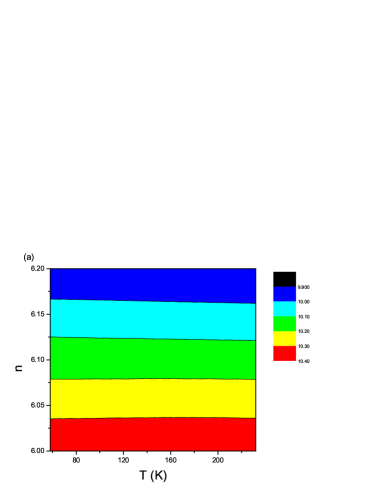
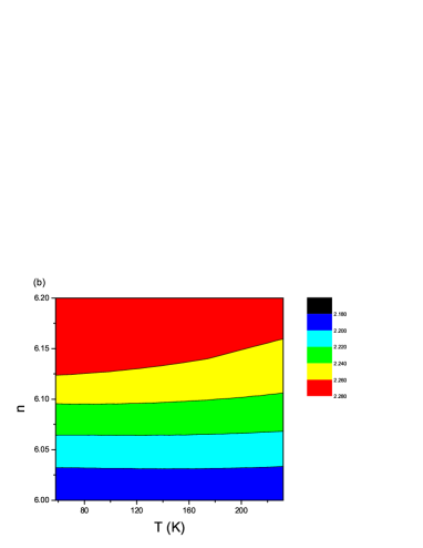
Figure 5: The temperature and doping dependence of the RPA-corrected in-plane orbital magnetic susceptibility(a) and the ratio between the in-plane and out-of-plane orbital magnetic susceptibility(b) for $6.0\leq n\leq 6.2$.

I.3 The temperature and doping dependence of the anisotropy ratio

Unlike the spin magnetic response, the orbital magnetic response is contributed by both intra-band and inter-band process. As a result, the orbital magnetic response is much less sensitive to the variation of temperature and doping concentration of the system. In Fig.5, we present the temperature and doping dependence of the RPA-corrected in-plane orbital magnetic susceptibility and the ratio between the in-plane and the out-of-plane orbital magnetic susceptibility.

From the figure it is clear that both quantities have only small temperature and doping dependence. More specifically, the relative change of the in-plane orbital magnetic susceptibility for $6.0\leq n\leq 6.2$ is only about 5 percent. The change in the anisotropy ratio is less than 0.1.

References

• (1) M. Yi, D. Lu, J.H. Chu, J. Analytis, A. Sorini, A. Kemper, B. Moritz, S.K. Mo, R.G. Moore, M. Hashimoto, W.S. Lee, Z. Hussain, T. Devereaux, I.R. Fisher, and Z.X. Shen, Proc. Natl. Acad. Sci. 108, 6878 (2011).
• (2) Y. Zhang, F. Chen, C. He, B. Zhou, B. P. Xie, C. Fang, W. F. Tsai, X. H. Chen, H. Hayashi, J. Jiang, H. Iwasawa, K. Shimada, H. Namatame, M. Taniguchi, J. P. Hu, D. L. Feng, Phys. Rev. B 83, 054510 (2011).
• (3) T. Shimojima, K. Ishizaka, Y. Ishida, N. Katayama, K. Ohgushi, T. Kiss, M. Okawa, T. Togashi, X.-Y. Wang, C.-T. Chen, S. Watanabe, R. Kadota, T. Oguchi, A. Chainani and S. Shin, Phys. Rev. Lett. 104, 057002 (2010).
• (4) T.M. Chuang, M.P. Allan, J. Lee, Y. Xi, N. Ni, S. Bud’ko, G.S. Boebinger, P.C. Canfield, and J.C. Davis, Science 327, 181 (2010).
• (5) J.H. Chu, J.G. Analytis, D. Press, K. De Greve, T.D. Ladd, Y. Yamamoto, I.R. Fisher, Phys. Rev. B 81, 214502 (2010).
• (6) J.H. Chu, J.G. Analytis, K. De Greve, P.L. McMahon, Z. Islam, Y. Yamamoto, and I.R. Fisher, Science 329, 824 (2010).
• (7) J.H. Chu, H.H. Kuo, J.G. Analytis and I.R. Fisher, Science 337, 710 (2012).
• (8) S. Kasahara, H. J. Shi, K. Hashimoto, S. Tonegawa, Y. Mizukami, T. Shibauchi, K. Sugimoto, T. Fukuda, T. Terashima, A.H. Nevidomskyy and Y. Matsuda Nature 486, 382 (2012).
• (9) C.C. Lee, W.G. Yin and W. Ku, Phys. Rev. Lett. 103, 267001 (2009).
• (10) W. Lv, J. Wu, and P. Phillips, Phys. Rev. B 80, 224506 (2009).
• (11) C.C. Chen, J. Maciejko, A.P. Sorini, B. Moritz, R. Singh and T. P. Devereaux, Phys. Rev. B 82, 100504 (2010).
• (12) W. Lv, F. Kruger, and P. Phillips, Phys. Rev. B 82, 045125 (2010).
• (13) A. H. Nevidomskyy, arxiv.org:1104.1747 (2011).
• (14) G. Wu, H. Chen, T. Wu, Y.L. Xie, Y.J. Yan, R.H. Liu, X.F. Wang, J.J. Ying and X.H. Chen, J. Phys.: Cond. Matter 20, 422201 (2008).
• (15) X.F. Wang, T. Wu, G. Wu, H. Chen, Y.L. Xie, J.J. Ying, Y.J. Yan, R.H. Liu, and X.H. Chen, Phys. Rev. Lett. 102, 117005 (2009).
• (16) J.Q. Yan, A. Kreyssig, S. Nandi, N. Ni, S.L. Bud’ko, A. Kracher, R.J. McQueeney, R.W. McCallum, T.A. Lograsso, A.I. Goldman, and P.C. Canfield, Phys. Rev. B 78, 024516 (2008).
• (17) Z. Li, D.L. Sun, C.T. Lin, Y.H. Su, J.P. Hu, G.Q. Zheng, Phys. Rev. B 83, 140506 (2011).
• (18) C. Xu, M. Muller, and S. Sachdev, Phys. Rev. B 78, 020501 (2008).
• (19) R. M. Fernandes, A. V. Chubukov, J. Knolle, I. Eremin, and J. Schmalian, Phys. Rev. B 85, 024534 (2012).
• (20) K. Kuroki, S. Onari, R. Arita, H. Usui, Y. Tanaka, H. Kontani, and H. Aoki, Phys. Rev. Lett.101, 087004 (2008).
• (21) Here $R_{x}(\pi)$ and $R_{y}(\pi)$ are the $\pi$ rotations along the $x$ and $y$ axis, $\sigma_{X}$ and $\sigma_{Y}$ are the mirror planes normal to the $X$ and $Y$ axis. $R_{x}(\pi)$, $\sigma_{X}$ and $\sigma_{Y}$ form a set of generators of the symmetry group $D_{2d}$ of the tetragonal phase and $R_{x}(\pi)$ and $R_{y}(\pi)$ form a set of generators of the symmetry group $D_{2}$ of the orthogonal phase.
• (22) R. Klingeler, N. Leps, I. Hellmann, A. Popa, U. Stockert, C. Hess, V. Kataev, H.J. Grafe, F. Hammerath, G. Lang, S. Wurmehl, G. Behr, L. Harnagea, S. Singh, and B. Büchner, Phys. Rev. B 81, 024506 (2010).
• (23) G.M. Zhang, Y.H. Su, Z.Y. Weng, D.H. Lee, and T. Xiang, EuroPhys. Lett. 86 37006 (2009).
• (24) S.P. Kou, T. Li, and Z.Y. Weng, EuroPhys. Lett. 88 17010 (2009).
• (25) M.M. Korshunov, I. Eremin, D.V. Efremov, D.L. Maslov, and A.V. Chubukov,Phys. Rev. Lett. 102, 236403 (2009).