Modeling the quantum interference signatures of the Ba ii D₂ 4554 Å line in the second solar spectrum

Abstract

Quantum interference effects play a vital role in shaping the linear polarization profiles of solar spectral lines. The Ba ii D₂ line at 4554 Å is a prominent example, where the $F$-state interference effects due to the odd isotopes produce polarization profiles, which are very different from those of the even isotopes that have no $F$-state interference. It is therefore necessary to account for the contributions from the different isotopes to understand the observed linear polarization profiles of this line. Here we do radiative transfer modeling with partial frequency redistribution (PRD) of such observations while accounting for the interference effects and isotope composition. The Ba ii D₂ polarization profile is found to be strongly governed by the PRD mechanism. We show how a full PRD treatment succeeds in reproducing the observations, while complete frequency redistribution (CRD) alone fails to produce polarization profiles that have any resemblance with the observed ones. However, we also find that the line center polarization is sensitive to the temperature structure of the model atmosphere. To obtain a good fit to the line center peak of the observed Stokes $Q/I$ profile, a small modification of the FALX model atmosphere is needed, by lowering the temperature in the line-forming layers. Because of the pronounced temperature sensitivity of the Ba ii D₂ line it may not be a suitable tool for Hanle magnetic-field diagnostics of the solar chromosphere, because there is currently no straightforward way to separate the temperature and magnetic-field effects from each other.

1 Introduction

The linearly polarized spectrum of the Sun known as the Second Solar Spectrum exhibits signatures of a number of physical processes not seen in the intensity spectrum and which may also be used to diagnose weak and turbulent magnetic fields that are inaccessible with the ordinary Zeeman effect. Many of the most prominent spectral lines in the Second Solar Spectrum, like Na i D₁ and D₂,  Ba ii D₁ and D₂, and Ca ii H and K, are governed by effects of quantum interference between states of different total angular momentum ($J$ or $F$ states). The profound importance of quantum interference for the formation of these lines was first demonstrated both observationally and theoretically by Stenflo (1980, see also ).

Quantum interference between the $J$-states governs the linear polarization signatures of atomic multiplets such as the Ca ii H and K, Na i D₁ and D₂, and Cr i triplet lines. The theory of such $J$-state interference was developed to include the effects of partial frequency redistribution (PRD) by Smitha et al. (2011, 2013). This theory was then applied successfully to model the linear polarization profiles of the Cr i triplet at 5204-5208 Å  by Smitha et al. (2012a).

When an atom possesses nuclear spin the $J$ states are split into $F$ states (hyperfine structure splitting). The quantum interference between the $F$ states produces depolarization in the line core. Examples of lines governed by $F$-state interference are the Na i D₂, Ba ii D₂, and Sc ii line at 4247 Å. The Ba ii D₂ line is due to the transition between the upper fine structure level $J=3/2$ and the lower level $J=1/2$ (see Figure 1(a)). In the odd isotopes of Ba, both the upper and lower levels undergo hyperfine structure splitting (HFS) due to the nuclear spin $I_{s}=3/2$, resulting in four upper and two lower $F$-states (see Figure 1(b)). The quantum interference between the upper $F$-states needs to be taken into account in the modeling of the Ba ii D₂ line. The odd isotopes contribute about 18% of the total Ba abundance in the Sun  (c.f. Table 3 of Asplund et al., 2009). The remaining 82% comes from the even isotopes, which are not subject to HFS (because $I_{s}=0$).

Figure 1: (a) represents the Ba ii model atom for the even isotopes, while for the odd isotopes the atomic model is modified by replacing two of the levels, ${}^{2}P_{3/2}$ and ${}^{2}S_{1/2}$, with their hyperfine structure components, as shown in (b). In (b), $I_{s}$ is the nuclear spin. The energy levels are not drawn to scale.

The intensity profile of the Ba ii D₂ line has earlier been studied extensively, for example by Holweger & Mueller (1974) and Rutten (1978, and the references cited therein). Some of these studies aimed at determining the solar abundance of Ba. Observations with the high precision spectro-polarimeter ZIMPOL by Stenflo & Keller (1997) clearly revealed the existence of three distinct peaks in the linear polarization $(Q/I)$ profiles of the Ba ii D₂ line. The nature of these peaks could subsequently be theoretically clarified by Stenflo (1997), who used the last scattering approximation to model the $Q/I$ profiles. It was demonstrated that the central $Q/I$ peak is due to the even isotopes of Ba, while the two side peaks are due to the odd isotopes.

Using a similar last scattering approximation, the magnetic sensitivity of the Ba line was explored by Belluzzi et al. (2007). Both these papers however did not account for radiative transfer or PRD effects. The potential of using the Ba ii D₂ line as a diagnostic tool for chromospheric weak turbulent magnetic fields and the important role of PRD were discussed by Faurobert et al. (2009), but the treatment was limited to the even Ba isotopes, for which HFS is absent. In contrast, our radiative-transfer treatment with PRD in the present paper includes both even and odd isotopes and the full effects of HFS with $F$-state interferences.

The theory of $F$-state interference with PRD in the non-magnetic collisionless regime was recently developed in Smitha et al. (2012b, herafter P1). The PRD matrix was also incorporated into the polarized radiative transfer equation. The transfer equation was then solved for the case of constant property isothermal atmospheric slabs. In the present paper we extend the work of P1 to solve the line formation problem in realistic 1-D model atmospheres in order to model the Ba ii D₂ line profile observed in a quiet region close to the solar limb.

The outline of the paper is as follows: In Section 2 we present the polarized radiative transfer equation which is suitably modified to handle several isotopes of Ba. In Section 3 we present the details of the observations. In Section 4 we discuss the model atom and the model atmosphere used. The results are presented in Section 5 with concluding remarks in Section 6.

2 Polarized line transfer equation with $F$-state interference

The polarization of the radiation field is in general represented by the full Stokes vector $(I,Q,U,V)^{\rm T}$. However, in the absence of a magnetic field Stokes $U$ and $V$ are zero in an axisymmetric 1-D atmosphere. Hence in a non-magnetic medium the Stokes vector $(I,Q)^{\rm T}$ is sufficient to express the polarization state of the radiation field. The transfer equation in the reduced Stokes vector basis (see Smitha et al., 2012a) is

$$\mu\frac{{\partial{\bm{\mathcal{I}}}(\lambda,\mu,z)}}{\partial z}=-k_{\rm tot}(\lambda,z)\left[{\bm{\mathcal{I}}}(\lambda,\mu,z)-{\bm{\mathcal{S}}}(\lambda,z)\right],$$ (1)

with positive $Q$ defined to represent linear polarization oriented parallel to the solar limb. The quantities appearing in Equation (1) are defined in the reference mentioned above. However, we need to generalize the previous definitions of opacity and source vector to handle even and odd isotope contributions together.

The total opacity $k_{\rm tot}(\lambda,z)=k_{l}(z)\phi_{g}(\lambda,z)+\sigma_{c}(\lambda,z)+k_{\rm th}(\lambda,z)$, where $\sigma_{c}$ and $k_{\rm th}$ are the continuum scattering and continuum absorption coefficients, respectively. In the present treatment, $k_{\rm th}$ also includes the contribution from the blend lines, which are assumed to be depolarizing and hence are treated in LTE. $k_{l}$ is the wavelength averaged absorption coefficient for the $J_{a}\to J_{b}$ transition. $J_{a}$ and $J_{b}$ are the electronic angular momentum quantum numbers of the lower and upper level, respectively. $\phi_{g}$ is the Voigt profile function written as

$$\phi_{g}(\lambda,z)=0.822~{}\phi_{e}(\lambda,z)+0.178~{}\phi_{o}(\lambda,z).$$ (2)

$\phi_{e}(\lambda,z)$ is the Voigt profile function for the even isotopes of Ba ii corresponding to the $J_{a}=1/2\to J_{b}=3/2$ transition in the absence of HFS. The profile function for the odd isotopes is $\phi_{o}(\lambda,z)$, which is the weighted sum of the individual Voigt profiles $\phi(\lambda_{F_{b}F_{a}},z)$ representing each of the $F_{a}\to F_{b}$ absorption transitions. Here $F_{a}$ and $F_{b}$ are the total angular momentum quantum numbers of the initial and the intermediate hyperfine split levels, respectively. $\phi_{o}(\lambda,z)$ is the same as $\phi_{\rm HFS}(\lambda,z)$ defined in Equation (7) of P1 and is given by

$$\phi_{o}(\lambda,z)=\bigg{[}\frac{2}{32}\phi(\lambda_{0\,1},z)+\frac{5}{32}\phi(\lambda_{1\,1},z)$$

$$+\frac{5}{32}\phi(\lambda_{2\,1},z)+\frac{1}{32}\phi(\lambda_{1\,2},z)$$

$$+\frac{5}{32}\phi(\lambda_{2\,2},z)+\frac{14}{32}\phi(\lambda_{3\,2},z)\bigg{]}.$$ (3)

The $17.8\%$ of $\phi_{o}(\lambda,z)$ in Equation (2) contains contributions from both the ¹³⁵Ba (6.6%) and ¹³⁷Ba (11.2%) odd isotopes.

The reduced total source vector $\bm{\mathcal{S}}(\lambda,z)$ appearing in Equation (1) is defined as

$$\bm{\mathcal{S}}(\lambda,z)=\frac{k_{l}(z)\bm{\mathcal{S}}_{l}(\lambda,z)+\sigma_{c}(\lambda,z)\bm{\mathcal{S}}_{c}(\lambda,z)}{k_{\rm tot}(\lambda,z)}$$

$$+\frac{k_{\rm th}(\lambda,z)\bm{\mathcal{S}}_{\rm th}(\lambda,z)+\epsilon~{}k_{l}(z)\phi_{g}(\lambda,z)\bm{\mathcal{S}}_{\rm th}(\lambda,z)}{k_{\rm tot}(\lambda,z)},$$

(4)

for a two-level atom with an unpolarized lower level. For the case of Ba ii D₂ it was shown by Derouich (2008) that any ground level polarization would be destroyed by elastic collisions with hydrogen atoms (see also Faurobert et al., 2009).

In Equation (4), $\bm{\mathcal{S}}_{\rm th}=(B_{\lambda},0)^{T}$, where $B_{\lambda}$ is the Planck function. ${\bm{\mathcal{S}}}_{l}(\lambda,z)$ is the line source vector defined as

$${\bm{\mathcal{S}}}_{l}(\lambda,z) = \int_{0}^{+\infty}\frac{1}{2}\int_{-1}^{+1}{\widetilde{{\bm{\mathcal{R}}}}(\lambda,\lambda^{\prime},z)}\hat{\Psi}(\mu^{\prime})$$ (5)

$$\times{\bm{\mathcal{I}}}(\lambda^{\prime},\mu^{\prime},z)\,d\mu^{\prime}\,d\lambda^{\prime},\ \ \ \ \$$

with

$${\widetilde{{\bm{\mathcal{R}}}}(\lambda,\lambda^{\prime},z)}=0.822~{}\widetilde{{\bm{\mathcal{R}}}_{e}}(\lambda,\lambda^{\prime},z)+0.178~{}\widetilde{{\bm{\mathcal{R}}}_{o}}(\lambda,\lambda^{\prime},z).$$ (6)

Here $\widetilde{{\bm{\mathcal{R}}}_{o}}(\lambda,\lambda^{\prime},z)$ is a $(2\times 2)$ diagonal matrix, which includes the effects of HFS for the odd isotopes. Its elements are $\widetilde{{\bm{\mathcal{R}}}_{o}}=$ diag $({\mathcal{R}}_{o}^{0},{\mathcal{R}}_{o}^{2})$, where ${\mathcal{R}}_{o}^{K}$ are the redistribution function components for the multipolar index $K$, containing both type-II and type-III redistribution of Hummer (1962). The expression for ${\mathcal{R}}^{K}$ is obtained by the quantum number replacement $L\rightarrow J;\ \ \ J\rightarrow F;\ \ \ S\rightarrow I_{s}$ in Equation (7) of Smitha et al. (2012b, see also and P1). In our present computations, we replace the type-III redistribution functions by CRD functions. We have verified that both of these give nearly identical results (see also Mihalas, 1978; Smitha et al., 2012a) and such a replacement drastically reduces the computation time. The redistribution matrix for the $17.8\%$ of the odd isotopes includes the contributions from the individual redistribution matrices for the ¹³⁵Ba and ¹³⁷Ba isotopes.

$\widetilde{{\bm{\mathcal{R}}}_{e}}(\lambda,\lambda^{\prime},z)$ is also a $(2\times 2)$ diagonal matrix for the even isotopes without HFS. Its elements ${\mathcal{R}}_{e}^{K}$ are the redistribution functions corresponding to the $J_{a}=1/2\to J_{b}=3/2\to J_{f}=1/2$ scattering transition. They are obtained by setting the nuclear spin $I_{s}=0$ in $\widetilde{{\bm{\mathcal{R}}}_{o}}(\lambda,\lambda^{\prime},z)$. An expression for $\widetilde{{\bm{\mathcal{R}}}_{e}}(\lambda,\lambda^{\prime},z)$ can be found in Domke & Hubeny (1988) and in Bommier (1997, see also ,  ) in the Stokes vector basis. It is the angle averaged versions of these quantities that are used in our present computations. As has been demonstrated in Supriya et al. (2013), the use of the angle-averaged redistribution matrix is sufficiently accurate for all practical purposes.

Like in Smitha et al. (2012b) we use the two branching ratios defined by

$$A=\frac{\Gamma_{R}}{\Gamma_{R}+\Gamma_{I}+\Gamma_{E}},$$

$$\!\!\!\!\!\!\!\!\!\!\!\!\!\!\!B^{(K)}=\frac{\Gamma_{R}}{\Gamma_{R}+\Gamma_{I}+D^{(K)}}\frac{\Gamma_{E}-D^{(K)}}{\Gamma_{R}+\Gamma_{I}+\Gamma_{E}}.$$ (7)

$\Gamma_{R}$ and $\Gamma_{I}$ are the radiative and inelastic collisional rates, respectively. $\Gamma_{E}$ is the elastic collision rate computed from Barklem & O’Mara (1998). $D^{(K)}$ are the depolarizing elastic collision rates with $D^{(0)}=0$. The $D^{(2)}$ is computed using (see Derouich, 2008; Faurobert et al., 2009)

$$D^{(2)}=6.82\times 10^{-9}n_{\rm H}(T/5000)^{0.40}$$

$$\!\!\!\!\!\!\!\!\!\!\!\!\!\!\!+7.44\times 10^{-9}(1/2)^{1.5}n_{\rm H}(T/5000)^{0.38}\exp(\Delta E/kT),$$

where $n_{\rm H}$ is the neutral hydrogen number density, $T$ the temperature, and $\Delta E$ the energy difference between the ${}^{2}P_{1/2}$ and ${}^{2}P_{3/2}$ fine structure levels. In the present treatment we neglect the collisional coupling between the ${}^{2}P_{3/2}$ level and the metastable ${}^{2}D_{5/2}$ level. The importance of such collisions for the line center polarization of Ba ii D₂ has been pointed out by Derouich (2008), who showed that the neglect of such collisions would lead to an overestimate of the line core polarization by $\sim 25\%$. This in turn would cause the microturbulent magnetic field $(B_{\rm turb})$ to be overestimated by $\sim 35\%$, as shown by Faurobert et al. (2009). However, the aim of the present paper is not to determine the value of $B_{\rm turb}$ but to explore the roles of PRD, HFS, quantum interferences, and the atmospheric temperature structure in the modeling of the triple peak structure of the Ba ii D₂ linear polarization profile.

Frequency coherent scattering is assumed in the continuum (see Smitha et al., 2012a) with its source vector given by

$${\bm{\mathcal{S}}}_{c}(\lambda,z)=\frac{1}{2}\int_{-1}^{+1}\hat{\Psi}(\mu^{\prime}){\bm{\mathcal{I}}}(\lambda,\mu^{\prime},z)\,d\mu^{\prime}.$$ (9)

The matrix $\hat{\Psi}$ is the Rayleigh scattering phase matrix in the reduced basis (see Frisch, 2007). The line thermalization parameter $\epsilon$ is defined by $\epsilon={\Gamma_{I}}/(\Gamma_{R}+\Gamma_{I})$. The Stokes vector $(I,Q)^{\rm T}$ can be computed from the irreducible Stokes vector $\bm{\mathcal{I}}$ by simple transformations given by (see Frisch, 2007)

$$I(\lambda,{\theta},z) = \mathcal{I}^{0}_{0}(\lambda,\mu,z)$$

$$+\frac{1}{2\sqrt{2}}(3\cos^{2}\theta-1)\mathcal{I}^{2}_{0}(\lambda,\mu,z),$$

$$Q(\lambda,\bm{\theta},z) = \frac{3}{2\sqrt{2}}(1-\cos^{2}\theta)\mathcal{I}^{2}_{0}(\lambda,\mu,z),\ \ \ \$$ (10)

where $\theta$ is the colatitude of the scattered ray. The scattering geometry is shown in Figure 1 of Anusha et al. (2011).

3 Observational details

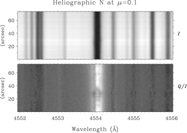
Figure 2: CCD image showing the $I$ and $Q/I$ spectra of the Ba ii D₂ line at $\mu=0.1$. The observations were obtained on June 3, 2008, with ZIMPOL-2 at the French THEMIS telescope on Tenerife.

The observed polarization profiles of the Ba ii D₂ line that are used in the present paper for modeling purposes were acquired by the ETH team of Stenflo on June 3, 2008, using their ZIMPOL-2 imaging polarimetry system (Gandorfer et al., 2004) at the THEMIS telescope on Tenerife. Figure 2 shows the CCD image of the data recorded at the heliographic north pole with the spectrograph slit placed parallel to the limb at $\mu=0.1$. The polarization modulation was done using Ferroelectric Liquid Crystal (FLC) modulators. The spectrograph slit was 1″  wide and 70″ long on the solar disk. The resulting CCD image has 140 pixels in the spatial direction and 770 pixels in the spectral direction. The effective pixel size was 0.5″spatially and 5.93 mÅ  spectrally. The observed profiles used to compare with the theoretical ones have been obtained by averaging the $I$ and $Q/I$ images in Figure 2 over the spatial interval 40″- 52″.

The recording presented in Figure 2 does not show much spatial variation along the slit, since it represents a very quiet region. However, recordings near magnetic regions made during the same observing campaign with ZIMPOL on THEMIS exhibit large spatial variations. It has long been known that all strong chromospheric scattering lines (like the Ca i 4227 Å, Na i D₂, Sr ii 4079 Å line, etc) have such spatial variations. Our observations confirm that the Ba ii D₂ line is no exception, which means that it is sensitive to the Hanle effect like the other chromospheric lines. Observations of spatial variations of this line have also been carried out by López Ariste et al. (2009) and Ramelli et al. (2009).

4 Modeling procedure

To model the polarization profiles of the Ba ii D₂ line we use a procedure similar to the one described in Holzreuter et al. (2005, see also ,  ,  ). It involves the computation of the intensity, opacity and collisional rates from the PRD-capable MALI (Multi-level Approximate Lambda Iteration) code developed by Uitenbroek (2001, referred to as the RH-code). The code solves the statistical equilibrium equation and the unpolarized radiative transfer equation self-consistently. The opacities and the collision rates thus obtained are kept fixed, while the reduced Stokes vector $\bm{\mathcal{I}}$ is computed perturbatively by solving the polarized radiative transfer equation with the angle-averaged redistribution matrices defined in Section 2.

Such a procedure requires a model atom and a model atmosphere as inputs to the RH-code. The details of the model atom and the atmosphere are discussed in the next subsections.

4.1 Model atom

Three different atom models are considered, two for the odd and one for the even isotope. The atom model for the even isotope (¹³⁸Ba) is given by the five levels of Figure 1(a), while for the odd isotopes (¹³⁵Ba and ¹³⁷Ba) the model is extended to include the hyperfine splitting as described by Figure 1(b). We neglect the contribution from other less abundant even isotopes. The wavelengths of the six hyperfine transitions for the odd isotopes are taken from Kurucz’ database and are listed in Table 1. These transitions are weighted with their line strengths given in Equation (3) (see Table 1).

4.2 Model atmosphere

We present the results computed for some of the standard realistic 1-D model atmospheres, like FALA, FALF, FALC (Fontenla et al., 1993) and FALX (Avrett, 1995). Among these four models FALF is the hottest and FALX the coolest. Their temperature structures are shown in the top panel of Figure 3. However, as will be discussed below, we find that a model atmosphere that is cooler than FALX is needed to fit the observed profiles. The new model, denoted $\overline{\rm FALX}$, is obtained by reducing the temperature of the FALX model by about 300 K in the height range 500 – 1200 km above the photosphere.

We have verified that such a modification of the FALX model does not significantly affect the intensity spectra. In contrast, the $Q/I$ spectra turn out to be very sensitive to such temperature changes. Like in Smitha et al. (2012a), we test the $\overline{\rm FALX}$ atmosphere by computing the limb darkening function for a range of wavelengths and $\mu$ values and compare it with the observed data from Neckel & Labs (1994). This is shown in the bottom panel of Figure 3. One can see that $\overline{\rm FALX}$ and the standard FALX fit the observed center-to-limb variation equally well. Therefore small modifications of the temperature structure to achieve a good fit to the observed $Q/I$ profile can be made without affecting the model constraints imposed by the intensity spectrum.

5 Results

In the following we discuss the modeling details and the need for a model atmosphere that is cooler than FALX. This helps us to evaluate the temperature sensitivity of the Ba ii D₂ line and its usefulness for magnetic-field diagnostics. In addition we demonstrate the profound role that PRD plays for the formation of the polarized line profile.

5.1 Modeling the Ba ii D₂ line profile

5.1.1 Modeling details

From the three Ba ii atom models described in Section 4.1 we obtain three sets of physical quantities (two for the odd isotopes and one for the even isotope) from the RH code. These quantities include line opacity, line emissivity, continuum absorption coefficient, continuum emissivity, continuum scattering coefficient, and the mean intensity. The mathematical expressions used to compute these various quantities for the even isotopes are given in Uitenbroek (2001). For the odd isotopes, the profile functions in these expressions are replaced by $\phi_{o}(\lambda,z)$ defined by Equation (3).

The three sets of quantities are then combined in the ratio of their respective isotope abundances and subsequently used as inputs to the polarization code.

5.1.2 Temperature sensitivity

The polarization profiles thus computed for the various model atmospheres are shown in Figure 4, displayed separately for the even, odd, and combined even-odd cases in three different panels. The Stokes $Q/I$ profiles in Figure 4 are computed by setting the total abundance of Ba in the Sun equal to the abundance of even isotopes in the first panel; the abundance of odd isotopes in the second panel; and a fractional abundance of even (82%) and odd (18%) isotopes in the third panel. The profiles in the first panel can be compared to the results presented in Figure 6 of Faurobert et al. (2009). As seen from the first panel, the amplitude of the central peak for the even isotopes is very sensitive to the temperature structure of the model atmosphere in contradiction with the conclusions of Faurobert et al. (2009). Also in their paper, the amplitude of the central peak obtained from the FALC model is larger than the one obtained from FALX, which is opposite to our findings (although it could be that the version of the FALC model they used is not identical to the one that we have used). However, the profile computed with the FALX model in first panel of Figure 4 for the even isotopes is in good agreement with the one given in their paper.

The profiles in the second panel of Figure 4, which represent the odd isotopes, also exhibit a similar large sensitivity to the choice of model atmosphere. Therefore the combined even-odd isotopes profiles in the third panel are also very sensitive to the temperature structure.

For the sake of clarity, let us point out that the combined $Q/I$ profiles in the bottom panel of Figure 4 differ profoundly from what one would obtain from a linear superposition of the corresponding profiles for the even and odd isotopes individually in the two other panels, in proportion to their isotope ratios. The reason is that the combination is highly non-linear, since the lines are formed in an optically thick medium (namely the radiative transfer effects). While the opacities and redistribution matrices are combined in a linear way as described by Equations (2) and (6), the even and odd isotopes blend with each other in the radiative transfer process, which makes the combination as it appears in the emergent spectrum highly non-linear.

The drastic depolarization of $Q/I$ in the line core has its origin in the polarizability factor $W_{2}$ of the odd isotopes. It is well known that the trough like suppression of $W_{2}$ in the line core for Ba ii is formed due to hyperfine structure for the odd isotopes (see Stenflo, 1997). In our radiative transfer calculations we have a superposition (in the proportion of the isotope ratios), of the trough-like scattering opacity of the odd isotopes, with the peak-like scattering opacity of the even isotopes. The shape of the $Q/I$ profile depends on the details of radiative transfer and PRD (see Equations (2)-(6)) namely on how these two scattering opacities non-linearly blend to produce the net result for the emergent radiation in the optically thick cases.

5.1.3 Need for the $\overline{\rm FALX}$ model

As seen from the last panel of Figure 4, the central peak is not well reproduced by any of the standard model atmospheres. All the models produce a dip at line center. Such a central dip is commonly due to the effects of PRD, caused by the properties of the type-II frequency redistribution. In the case of Ba ii D₂, the contribution to this central dip comes mainly from the even isotopes, as shown in Figure 5. The three rows in this figure represent the even, odd and combined even-odd cases, respectively, for the FALX model atmosphere. The first column shows the profiles computed with only type-II redistribution, the second column those computed with CRD only. The CRD profiles are obtained by setting the branching ratios $A=0$ and $B^{(K)}=(1-\epsilon)$. None of the CRD profiles shows a central dip.

The occurrence and nature of this central dip has been explored in detail in Holzreuter et al. (2005), who showed that its magnitude is strongly dependent on the choice of atmospheric parameters. This behavior is also evident from Figure 4. The cooler the atmosphere, the smaller is the central dip. The dip is often smoothed out by instrumental and macro-turbulent broadening. However, the profiles in Figure 4 have already been smeared with a Gaussian function having a full width at half maximum (FWHM) of 70 mÅ. The dip could be suppressed by additional smearing, but such large smearing would also suppress the observed side peaks of the odd isotopes and would make the intensity profile inconsistent with the observed one. The value 70 mÅ has been chosen to optimize the fit, but it is also consistent with what we expect based on the observing parameters and turbulence in the chromosphere.

The failure of all the tried standard model atmospheres therefore leads us to introduce a new model with a modified temperature structure, which is cooler than the standard FALX model. The details of the new cooler $\overline{\rm FALX}$ model has been given in Section 4.2. This new model atmosphere succeeds in giving a good fit to both the intensity and the polarization profiles, as shown in Figure 6. To simulate the effects of spectrograph stray light on the intensity and polarization profiles we have applied a spectrally flat unpolarized background of 4% of the continuum intensity level to the theoretical $(I,Q/I)$ profiles. For a good $Q/I$ line center fit, we find that it is necessary to include Hanle depolarization from a non-zero magnetic field. Our theoretical profiles are based on a micro-turbulent magnetic field of strength $B_{\rm turb}$ with an isotropic angular distribution. Our best fit to the $Q/I$ profile corresponds to a field strength of $B_{\rm turb}$ = 2 G.

5.2 The importance of PRD

The importance of PRD in modeling the Ba ii D₂ line has already been demonstrated in Faurobert et al. (2009), although by only considering the even isotopes. Figure 5 demonstrates the importance of PRD for both the odd and the even isotopes. As seen from the second column of this figure, the $Q/I$ profiles for the odd isotopes when computed exclusively in CRD do not produce any side peaks, while the profiles computed with type-II redistribution exhibits such peaks. Also, by comparing the $Q/I$ profiles for the even isotopes in the first row, we see that CRD fails to generate the needed line wing polarization. A comparison between the observed profiles and the theoretical profiles based on CRD alone (dotted line) and on full PRD (dashed line) for the $\overline{\rm{FALX}}$ model is shown in Figure 7. While the intensity profile can be fitted well using either PRD or CRD, the polarization profile cannot be fitted at all with CRD alone. PRD is therefore essential to model the $Q/I$ profiles of the Ba ii D₂ line.

6 Conclusions

In the present paper we have for the first time tried to model the polarization profiles of the Ba ii D₂ line by taking full account of PRD, radiative transfer, and HFS effects. We use the theory of $F$-state interference developed in P1 in combination with different atom models representing different isotopes of Ba ii and various choices of model atmospheres. Applications of the well known standard model atmospheres FALF, FALC, FALA, and FALX fail to reproduce the central peak, and instead produce a central dip mainly due to PRD effects. We have shown that in the case of Ba ii D₂ the central dip is reduced by lowering the temperature of the atmospheric model. We can therefore achieve a good fit to the observed polarization profile by slightly reducing the temperature of the FALX model.

In modeling the Ba ii D₂ line we account for the depolarizing effects of elastic collisions with hydrogen atoms but neglect the alignment transfer between the ${}^{2}P_{3/2}$ level and the metastable ${}^{2}D_{5/2}$ level. It has been shown by Derouich (2008) that this alignment transfer affects the line center polarization and is needed for magnetic field diagnostics. The purpose of the present paper is however not to determine magnetic fields but to clarify the physics of line formation.

We demonstrate that PRD is essential to reproduce the triple peak structure and the line wing polarization of the Ba ii D₂ line, but find that the line center polarization is very sensitive to the temperature structure of the atmosphere, which contradicts the conclusions of Faurobert et al. (2009), who find that the barium line is temperature insensitive and therefore suitable for Hanle diagnostics. This contradiction illustrates that a full PRD treatment as done in the present paper, including the contributions from both the even and odd isotopes, is necessary to bring out the correct temperature dependence of the line. The large temperature sensitivity of the Ba ii D₂ line makes it rather unsuited for magnetic-field diagnostics, since there is no known straightforward way to separate the temperature and magnetic-field effects for this line.

Table 1: Wavelengths (Å) of the hyperfine transitions for the odd isotopes of Ba ii

$F_{a}$	$F_{b}$	135Ba	137Ba	Line strength
1	0	4553.999	4553.995	0.15625
1	1	4554.001	4553.997	0.06250
1	2	4554.001	4553.998	0.15625
2	1	4554.046	4554.049	0.43750
2	2	4554.059	4554.051	0.15625
2	3	4554.050	4554.052	0.03125

Figure 3: Top panel: The temperature structure of some of the standard model atmospheres. $\overline{\rm{FALX}}$ represents the model for which the temperature is reduced by about 300 K over a 700 km range around the height of formation of the Ba ii D₂ line. Bottom panel: Comparison between the observed center-to-limb variation (CLV) of the continuum intensity and the predictions from different model atmospheres including $\overline{\rm FALX}$ for a wide range of wavelengths from the violet to the IR region of the spectrum. For all the $\mu$ values the dashed and the dash-triple dotted lines are practically indistinguishable as the models FALX and $\overline{\rm FALX}$ produce nearly identical fits.

Figure 4: Comparison between the observed $Q/I$ profile and the theoretical profiles for some of the standard model atmospheres, separately displayed for the even, odd, and combined even-odd cases. The theoretical profiles represent the non-magnetic case and have been smeared with a Gaussian having a full width at half maximum (FWHM) of 70 mÅ to account for instrumental and macro-turbulent broadening.

Figure 5: Theoretical $Q/I$ profiles computed for the non-magnetic FALX model for the even (first row), odd (second row), and combined even-odd (third row) isotopes, with only type-II frequency redistribution (first column) and only complete frequency redistribution CRD (second column). A prominent central dip is present for the type-II redistribution profiles although they have been smeared with a Gaussian having FWHM = 70 mÅ.

Figure 6: Fit to the observed profile using the $\overline{\rm{FALX}}$ model with and without a micro-turbulent magnetic field $B_{\rm turb}$. The theoretical profiles have been smeared using a Gaussian with FWHM = 70 mÅ.

Figure 7: Comparison between the observed Stokes profiles and the profiles computed with CRD (dotted line) and PRD (dashed line) for the $\overline{\rm FALX}$ model. The theoretical profiles have been smeared with a Gaussian having FWHM = 70 mÅ. The strength of the micro-turbulent magnetic field $B_{\rm turb}$ has been chosen to be 2 G for the PRD and 5 G for the CRD profiles. The dashed line in this figure is same as the dashed line in Figure 6.

References

- Anusha et al. (2010) Anusha, L. S., Nagendra, K. N., Stenflo, J. O., Bianda, M., Sampoorna, M., Frisch, H., Holzreuter, R., & Ramelli, R. 2010, ApJ, 718, 988
- Anusha et al. (2011) Anusha, L. S., et al. 2011, ApJ, 737, 95
- Asplund et al. (2009) Asplund, M., Grevesse, N., Sauval, A. J., & Scott, P. 2009, ARA&A, 47, 481
- Avrett (1995) Avrett, E. H. 1995, in Infrared tools for solar astrophysics: What’s next?, ed. J. R. Kuhn & M. J. Penn, 303–311
- Barklem & O’Mara (1998) Barklem, P. S., & O’Mara, B. J. 1998, MNRAS, 300, 863
- Belluzzi et al. (2007) Belluzzi, L., Trujillo Bueno, J., & Landi Degl’Innocenti, E. 2007, ApJ, 666, 588
- Bommier (1997) Bommier, V. 1997, A&A, 328, 706
- Derouich (2008) Derouich, M. 2008, A&A, 481, 845
- Domke & Hubeny (1988) Domke, H., & Hubeny, I. 1988, ApJ, 334, 527
- Faurobert et al. (2009) Faurobert, M., Derouich, M., Bommier, V., & Arnaud, J. 2009, A&A, 493, 201
- Fontenla et al. (1993) Fontenla, J. M., Avrett, E. H., & Loeser, R. 1993, ApJ, 406, 319
- Frisch (2007) Frisch, H. 2007, A&A, 476, 665
- Gandorfer et al. (2004) Gandorfer, A. M., Steiner, H. P. P. P., Aebersold, F., Egger, U., Feller, A., Gisler, D., Hagenbuch, S., & Stenflo, J. O. 2004, A&A, 422, 703
- Holweger & Mueller (1974) Holweger, H., & Mueller, E. A. 1974, Sol. Phys., 39, 19
- Holzreuter et al. (2005) Holzreuter, R., Fluri, D. M., & Stenflo, J. O. 2005, A&A, 434, 713
- Hummer (1962) Hummer, D. G. 1962, MNRAS, 125, 21
- López Ariste et al. (2009) López Ariste, A., Asensio Ramos, A., Manso Sainz, R., Derouich, M., & Gelly, B. 2009, A&A, 501, 729
- Mihalas (1978) Mihalas, D. 1978, Stellar atmospheres /2nd edition/
- Nagendra (1994) Nagendra, K. N. 1994, ApJ, 432, 274
- Neckel & Labs (1994) Neckel, H., & Labs, D. 1994, Sol. Phys., 153, 91
- Ramelli et al. (2009) Ramelli, R., Bianda, M., Trujillo Bueno, J., Belluzzi, L., & Landi Degl’Innocenti, E. 2009, in Astronomical Society of the Pacific Conference Series, Vol. 405, Solar Polarization 5: In Honor of Jan Stenflo, ed. S. V. Berdyugina, K. N. Nagendra, & R. Ramelli, 41
- Rutten (1978) Rutten, R. J. 1978, Sol. Phys., 56, 237
- Sampoorna (2011) Sampoorna, M. 2011, ApJ, 731, 114
- Smitha et al. (2013) Smitha, H. N., Nagendra, K. N., Sampoorna, M., & Stenflo, J. O. 2013, J. Quant. Spec. Radiat. Transf., 115, 46
- Smitha et al. (2012a) Smitha, H. N., Nagendra, K. N., Stenflo, J. O., Bianda, M., Sampoorna, M., Ramelli, R., & Anusha, L. S. 2012a, A&A, 541, A24
- Smitha et al. (2011) Smitha, H. N., Sampoorna, M., Nagendra, K. N., & Stenflo, J. O. 2011, ApJ, 733, 4
- Smitha et al. (2012b) Smitha, H. N., Sowmya, K., Nagendra, K. N., Sampoorna, M., & Stenflo, J. O. 2012b, ApJ, 758, 112
- Stenflo (1980) Stenflo, J. O. 1980, A&A, 84, 68
- Stenflo (1997) —. 1997, A&A, 324, 344
- Stenflo & Keller (1997) Stenflo, J. O., & Keller, C. U. 1997, A&A, 321, 927
- Supriya et al. (2013) Supriya, H. D., Smitha, H. N., Nagendra, K. N., Ravindra, B., & Sampoorna, M. 2013, MNRAS, 429, 275
- Uitenbroek (2001) Uitenbroek, H. 2001, ApJ, 557, 389