Decay behavior of localized states at reconstructed armchair graphene edges

Abstract

Density functional theory calculations are used to investigate the electronic structures of localized states at reconstructed armchair graphene edges. We consider graphene nanoribbons with two different edge types and obtain the energy band structures and charge densities of the edge states. By examining the imaginary part of the wavevector in the forbidden energy region, we reveal the decay behavior of the wavefunctions in graphene. The complex band structures of graphene in the armchair and zigzag directions are presented in both tight-binding and first-principles frameworks.

I Introduction

One-dimensional boundaries are a distinctive feature of finite-sized graphene, which means that an investigation and understanding of the electronic properties of graphene edges are of particular importance. Even before the first production of graphene from graphite by mechanical exfoliation in 2004graphene , the edge state was shown to be a typical example of the manifestation of the topological characteristics of a bulk bandtopology . The boundary or edge effects become more significant for practical applications as the size of graphene in a device becomes smaller. Real graphene edges are usually passivated with functional groups, transition metals, or hydrogen atoms depending on the specific purpose, but even without these external chemicals or elements, reconstruction of the graphene edge itself has been observedKoskinen . How deeply the edge-induced state penetrates the bulk determines the decay length and extent of the state localization.

According to Bloch’s theorem, the eigenstates of the single-electron Schrödinger equation in a crystal satisfy $\psi({\bf r})=e^{i{\bf k}\cdot{\bf r}}u_{n{\bf k}}({\bf r}),$ where $u_{n{\bf k}}$ is a function that has the same periodicity as the crystal, $n$ is the band index, and k is the wavevector. In the case of an infinite crystal, the Born–von Karman cyclic boundary conditionsAshcroft restrict the wavevectors to real quantities. However, complex Bloch k vectors are allowed for finite crystals, and the complex band structure of a periodic system is the conventional band structure extended to complex Bloch k vectors. Near a crystal surface or interface, one can match a wavefunction with a complex k between the inside and outside of the crystal region, and thus surface or interface evanescent states ariseKohn ; Heine1 ; Heine2 ; Chang .

The complex band structure concept can also be adopted for graphene edges; the properties of the edge states are closely related to the band structure of infinite graphene. If we know the dispersion relation of the edge state that can be accurately calculated in a relatively narrow graphene nanoribbon (GNR), then this approach allows us to predict the decay behavior of the edge state in semi-infinite graphene, combined with the complex band structure of infinite (bulk) graphene. The wavevector can be split into a component parallel to the edge, $k_{||}$, which is conserved during scattering, and a perpendicular component, $k_{\perp}$. Then, for each real $k_{||}$, the dispersion relation $E=E(k_{\perp})$ allows a complex $k_{\perp}=k^{\prime}+i\kappa$, where $k^{\prime}$ and $\kappa$ are real. We refer to the imaginary part $\kappa$ as the decay parameter.

In this paper, we focus on reconstructed armchair graphene edges. A perfect armchair graphene edge has no localized edge state since its one-dimensional bulk Hamiltonian $H_{k_{||}}(k_{\perp})$ is topologically trivial for any $k_{\|}$ valuetopology . However, reconstructed armchair edges may have localized edge states because of the modification of the geometries and hopping properties. Using first-principles calculations, we show that the possible localized edge states have decay behaviors that are associated with the complex band structure of graphene in the bulk. Near a graphene edge, the solution for an edge state should be matched to the bulk graphene wavefunction with complex k. Therefore, to investigate the decay pattern of the localized edge states, we need to calculate the complex band structure of graphene. In addition, we provide analytic solutions to the complex band structures for both the armchair and zigzag directions using the nearest-neighbor tight-binding method.

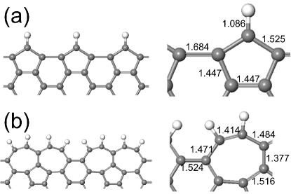
Figure 1: (Color online) Model structures of reconstructed armchair edges: (a) pentagonal armchair edge with missing carbon atoms [ac(56)], and (b) reconstructed armchair edge in which two heptagons created by the Stone–Wales transformation share a side [ac(677)]. The bond lengths (in Å) at the graphene edges are shown in the right panel. The gray and white spheres are carbon and hydrogen atoms, respectively.

II Computational details

We performed density functional theory calculations within the generalized gradient approximation (GGA) for the exchange-correlation functional. The Perdew–Burke–Ernzerhof (PBE) functional formPBE was adopted for the GGA. Ionic potentials were described by the projector augmented wave (PAW)PAW method implemented in the Vienna Ab Initio Simulation Package (VASP)VASP . To mimic semi-infinite graphene, we chose GNRs that have an ac(56)- or ac(677)-type edgeKoskinen on one side and a perfect armchair edge on the other side. The widths of our model GNRs with the ac(56)- and ac(677)-type edges were $\sim$5 and $\sim$6 nm, respectively. We used 24 and 12 k points to sample the Brillouin zone (BZ) in the edge direction in the respective edge geometries. A plane-wave energy cutoff of 400 eV was used for the structural relaxation, which continued until the atomic forces were smaller than 20 meV/Å. The size of the unit cell of the ac(677)-type edge was twice that of the ac(56)-type edge along the ribbon axis, as shown in Fig. 1. The supercells contained 91 and 204 carbon atoms for the GNRs with the ac(56)- and ac(677)-type edges, respectively.

To calculate the complex band structures in the primitive cell, we employed the Quantum Espresso packagepwscf . The Vanderbilt ultrasoft pseuopotentialVanderbilt was generated through the Rappe–Rabe–Kaxiras–Joannopoulos (RRKJ)RRKJ pseudo-wavefunction construction scheme. The kinetic energy cutoff was 30 Ry. From the symmetry of the hexagonal cell, the net force exerted on each carbon atom was zero, and the lattice parameters were optimized by the Birch–Murnaghan equation of stateMurnaghan ; Birch . To consider the conservation of ${\bf k}_{||}$ in the presence of the edge and the crystallographic direction to the edge, we considered a rectangular unit cell containing 4 carbon atoms for the armchair and zigzag edges. This is the smallest unit cell with the lattice vector aligned along ${\bf k}_{||}$. All results are obtained in the rectangular unit cell in the present study.

For the k point sampling, 24 $\times$ 24 $\times$ 1 k points were chosen in the Monkhorst–Pack schemeMonkhorst-Pack .

In the tight-binding approximation, the Hamiltonian of a graphene monolayer is expressed as

$$H=\sum_{<i,j>}\left(tc_{i}^{\dagger}c_{j}+{\rm h.c.}\right),$$ (1)

where $\sum_{<i,j>}$ sums over only nearest-neighbor pairs, $c_{i}^{\dagger}$($c_{i}$) is the creation (annihilation) operator, and h.c. indicates the Hermitian conjugate. Here, $t$ is the nearest-neighbor hopping energy ($=-2.88$ eV).

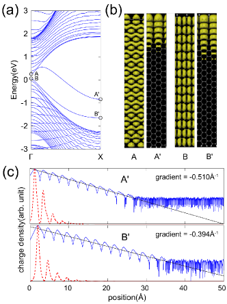
Figure 2: (Color online) (a) Band structure of a GNR with an ac(56) edge, and (b) electronic densities of two edge-related states. The labels A (B) and A^′ (B^′) indicate electronic densities in the same band at $\Gamma$ and X, respectively. (c) Plane-averaged electron densities (red) and their semilog plots (blue) of the GNR with the ac(56) edge showing an exponentially decaying character; the gradients of the fitted curves give the decay parameters in units of Å^-1. The position indicated on the horizontal axis is the distance from the hydrogen atom at the ac(56) edge to the middle of the ribbon.

III Results and discussion

The optimized structures of the two GNRs are shown in Fig. 1. The ac(56) model shows a pentagonal reconstruction of the armchair edge (with a connecting hexagon) that requires the diffusion of carbon atomsKoskinen . The ac(677) modelKoskinen ; GDLee , however, shows a reconstruction in which two heptagons share a side (a carbon bond). Unlike the models of Koskinen et al.Koskinen , our graphene edges are passivated with hydrogen atoms.

Figure 2 shows the electronic band structure and charge densities at $\Gamma$ and X in the armchair GNR with the pentagonal reconstruction, ac(56). Two bands labeled as AA^′ and BB^′ are seen in the forbidden energy band. Because of the added carbon atoms, one additional band, labeled as AA^′, appears near the Fermi level. In terms of the tight-binding calculation, this corresponds to the inclusion of new basis functions. At the zone boundary (X), the edge states exist as deep levels in the forbidden energy region so that they are more localized than the edge states at the $\Gamma$ point. The overlapping of a localized state with the bulk states in k-space is generally referred to as surface resonanceKolasinski ; the localized state penetrates the bulk and couples strongly to the bulk states. Thus, the electronic states labeled A and B for the ac(56) model are extended GNR states with enhanced amplitudes near the edge.

In our previous studyPNAS of the reconstructed armchair edge ac(56), we showed that the edge hopping energy $t_{0}$ at the pentagon is approximately $-2$ eV by using the maximally localized Wannier function methodMarzari . In ideal graphene, the hopping energy $t$ is $-2.88$ eV, which thus corresponds to boundary softening ($t_{0}<t$). Li et al.WLi showed that edge-hopping modulation may give rise to the edge state at the perfect armchair edge.

We can estimate the decay lengths of edge states from a calculation of the energy levels of a relatively narrow GNR because the interaction between the two edges of the nanoribbon quickly decreases as the width of the ribbon increases; the energies of the edge states then rapidly converge to the semi-infinite limit. The decay length $\lambda_{\text{decay}}(=2\pi/\kappa)$ is obtained from the decaying factor $e^{-\kappa r_{\perp}}$, where $r_{\perp}$ is the perpendicular direction to the boundary. The estimated decay lengths are 1.23 and 1.59 nm for states A^′ and B^′, respectively, as obtained from gradients of $-$0.510 and $-$0.394 Å^-1, respectively, in the semilog plot of the decaying electronic densities in Fig. 2. The shorter decay length of state A^′ can also be seen in Fig. 2(b).

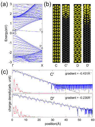
Figure 3: (Color online) (a) Band structure of a GNR with the ac(677) edge, and (b) electronic densities of two edge-related states. The labels C (D) and C^′ (D^′) indicate electronic densities in the same band at $\Gamma$ and X, respectively. (c) Plane-averaged electron densities (red) and their semilog plots (blue) for the GNR with the ac(677) edge showing an exponential decaying character; the gradients of fitted curved give the decay parameters in units of Å^-1. The position indicated on the horizontal axis is the distance from the hydrogen atom at the ac(677) edge to the middle of the ribbon.

Figure 3 shows the edge states near the Fermi level at the ac(677)-reconstructed edge. The reconstruction can be understood as an array of Stone–Wales defects, as this geometry is obtained by rotating particular carbon–carbon bonds by $90^{\circ}$. The Stone–Wales defect in carbon nanotubes is known to be able to form two quasi-bound statesHChoi that are characterized as bonding and anti-bonding states in the rotated carbon dimerGKim . Figure 3(a) shows that a nearly flat band, labeled as CC^′, is unoccupied and may act as an acceptor level. In Fig. 3(b), the electronic charge densities of states C^′ and D have distinct anti-bonding and bonding characteristics in the rotated carbon dimer, respectively. Although the energy dispersion of the CC^′ band is nearly flat, the decay lengths of the edge states vary significantly depending on $k_{||}$ in the edge direction. In fact, near the $\Gamma$ point, the edge state is located inside an allowed energy band so that it is not a localized state due to mixing with the extended states. For state C^′, the energy level is deep into the bulk energy gap. Consequently, its electronic charge density is strongly localized at the edge and has a decay length of 1.46 nm. In contrast, the energy level of state D^′ is so close to the valence band edge over the whole $k_{\|}$ range that the decay length is relatively long (2.73 nm). The difference in the decay lengths can also be seen Figure 3(b).

We can deduce the decay length of an edge state from its energy level when the Bloch wavevector k is assumed to be a complex number. The general procedure for considering the complex wavevector is as follows: The crystal translational symmetry produces a wavevector k a good quantum number, and the bulk Hamiltonian can be decoupled for each k. The secular equation

$$det[E-H({\bf{k}})]=det[E-H(k_{\|},k_{\perp})]=0$$ (2)

then gives the energy levels and Bloch wavefunctions of the crystal. In this case, k is regarded as a parameter. If we now also regard the energy and $k_{\|}$ as parameters and solve the secular equation with respect to $k_{\perp}$, then the secular equation becomes a polynomial of $k_{\perp}$ in generalsuperlattice . In line with the fundamental theorem of algebra, the polynomial has the same number of zeroes (including complex values) as the degree of the polynomial independent of the energy and $k_{\|}$. This means that whenever there is a band edge where the real band begins to vanish, a corresponding complex band appears from the band edge. In view of the single-particle Schrödinger equation, the wavefunction at the boundary should be matched to a linear combination of bulk wavefunctions (including waves having complex wavevectors). When this linear combination does not include any wavefunctions with a purely real wavevector, it forms surface or interface evanescent states.

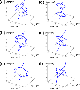
Figure 4: (Color online) Tight-binding complex band structures of graphene in the armchair direction (a) $k_{||}=0$, (b) $k_{||}=\frac{1}{4}G_{||}$, and (c) $k_{||}=\frac{1}{2}G_{||}$, where $G_{\|}=\frac{2\pi}{3a}$, and $a$ is the carbon–carbon bond length (= 1.42Å), and the zigzag direction (d) $k_{||}=0$, (e) $k_{||}=\frac{1}{3}G_{||}$, and (f) $k_{||}=\frac{1}{2}G_{||}$, where $G_{\|}=\frac{2\pi}{\sqrt{3}a}$. The hopping energy is set to $-2.88$ eV.

Near the band edge, the behavior of the complex band is easily derived from an effective Hamiltonian. Usually, the real band has an approximately quadratic dispersion near its edge, and the effective Hamiltonian can be expressed as

$$H({\bf{k}})=\frac{\hbar^{2}|{\bf k}|^{2}}{2m}+E_{0}=\frac{\hbar^{2}}{2m}(k_{\|}^{2}+k_{\perp}^{2})+E_{0}.$$ (3)

For a given $k_{\|}=k_{0}$ and $E$, solving this Hamiltonian with respect to $k_{\perp}$ gives the complex band structure. When $E$ lies in the forbidden energy regime ($E<\frac{\hbar^{2}k_{0}^{2}}{2m}+E_{0}$),

$$k_{\perp}=\pm i\sqrt{k_{0}^{2}-\frac{2m(E-E_{0})}{\hbar^{2}}},$$ (4)

and the decaying parameter $k_{\perp}\propto\sqrt{E_{0}^{\prime}-E}$, where $E_{0}^{\prime}\equiv\frac{\hbar^{2}k_{0}^{2}}{2m}+E_{0}$ is the band edge for a given $k_{\|}$.

The nearest-neighbor tight-binding model provides the essential features of the complex band structure and assists in understanding the overall structures of the complex bands We can solve the secular equation of a $4\times 4$ tight-binding matrix for $k_{\perp}$ and obtain analytic solutions for specific $k_{||}$ and $E$ values. Within the framework of the tight-binding approximation, we can obtain the decay parameters for states A^′, B^′, C^′, and D^′ in the ac(56) and ac(677) edges (Figs. 2 and 3). At $k_{||}=\frac{1}{2}G_{\|}=\frac{\pi}{3a}$, where $a$ is the carbon–carbon bond length, the decay parameters for states A^′ and B^′ are 0.375 and 0.325 Å^-1, respectively. On the other hand, the decay parameters for states C^′ and D^′ are 0.297 and 0.196 Å^-1, respectively, at $k_{||}=\frac{1}{4}G_{\|}=\frac{\pi}{6a}$. Although the nearest-neighbor tight-binding method can provide overall structures of the complex band, there is a discrepancy between the decay lengths calculated using the tight-binding and first-principles methods for each state. Unlike the real band structure that can accurately describe the energy region near the Fermi level, the complex band structure derived from the tight-binding calculation is not accurate because it depends sensitively on the energy positions of the band edges at each $k_{\|}$, which is usually far from the Fermi level.

In Fig. 4, the tight-binding complex band structures are plotted for particular $k_{\|}$ values in both the armchair and zigzag directions. In both cases, the complex band has a quadratic shape near the X point (the band edge), the localization becomes stronger further away from the band edge, and reaches a maximum deep inside the band gap. At any energy around the Fermi level, there are always four (two) $\pi$-bands in the graphene in the armchair (zigzag) directions. This feature is related to the different number of maximum scattering channels in the two directions because the energy and crystal momentum along the direction parallel to the edge are conserved during electron scatteringPNAS .

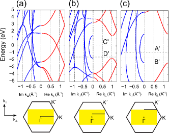
Figure 5: (Color online) First-principles complex band structures of graphene in the armchair direction. Real and imaginary bands are plotted along the positive and negative axes, respectively. The lower hexagons are the BZ of graphene, and the yellow rectangles denote the BZ if a doubled unit cell of graphene is considered for the armchair cell construction. The band structures are plotted along line segments. From the left panel, (a) $k_{||}=0$, (b) $k_{||}=\frac{1}{4}G_{||}$, and (c) $k_{||}=\frac{1}{2}G_{||}$, where $G_{\|}=\frac{2\pi}{3a}$. In (b) and (c), the dotted lines represent the energy levels of the localized edge states A^′, B^′, C^′, and D^′ in Figs. 2 and 3, respectively.

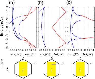
Figure 6: (Color online) First-principles complex band structures of graphene in the zigzag direction. The yellow rectangle denotes the BZ of a doubled unit cell of graphene for the zigzag rectangular cell construction. From the left panel, (a) $k_{||}=0$, (b) $k_{||}=\frac{1}{3}G_{||}$, and (c) $k_{||}=\frac{1}{2}G_{||}$, where $G_{\|}=\frac{2\pi}{\sqrt{3}a}$, and $a$ is the carbon–carbon bond length.

Complex band structures of graphene in the armchair direction calculated from first principles in a plane-wave basis are shown in Fig. 5 for three $k_{||}$ values ($k_{||}=0$, $\frac{1}{4}G_{||}$, and $\frac{1}{2}G_{||}$), where $G_{\|}=\frac{2\pi}{3a}$. In principle, any edge state in the bulk region can be represented by a linear combination of wavefunctions that correspond to a complex band of the same energy, and in practice, the dominant contribution comes from the first few bands with long decay lengths. Furthermore, in case of the graphene edge, the first complex band with the longest decay length is composed of $\pi$-electrons and determines the decay length of the edge state. The energy levels of the edge states of the ac(56) edge at the X point (A^′ and B^′ in Fig. 2) are $-$0.84 and $-$1.64 eV, respectively, and the corresponding decay parameters ($\kappa$) are 0.255 and 0.207 Å^-1, as shown in Fig. 5(c). Because the charge density is given by the squared magnitude of the wavefunction, the decay parameters ($\kappa$) should be doubled for comparison with the gradients in Fig. 2: this gives decay lengths of 0.510 and 0.394 Å^-1 for A^′ and B^′, respectively. The small difference is attributed to the finite size effect of the ribbon width.

In the case of the ac(677) edge, both $k_{\|}=\frac{1}{4}G_{\|}$ and $k_{\|}=\frac{1}{2}G_{\|}$ should be considered due to the doubling of the armchair unit cell. The energy levels of the C^′ and D^′ states in Fig. 3 are 0.14 and $-$1.55 eV, respectively, and the corresponding decay parameters are 0.219 and 0.110 Å^-1 at $k_{\|}=\frac{1}{4}G_{\|}$ and 0.249 and 0.216 Å^-1 at $k_{\|}=\frac{1}{2}G_{\|}$. Because the complex bands at $k_{\|}=\frac{1}{4}G_{\|}$ have smaller decay parameter, the decay lengths are determined by those bands. As mentioned earlier, the ac(677)-type edge has a lattice parameter that is twice that of the ac(56)-type edge, and the band edge corresponding to the ac(677) edge is at $k_{\|}=\frac{1}{4}G_{\|}$. If the $\kappa$ values at $k_{\|}=\frac{1}{4}G_{\|}$ is doubled, then agreement with the gradients of the charge densities (0.431 Å^-1 for C^′ and 0.230 Å^-1 for D^′) in Fig. 3(c) is obtained. Here, it is necessary to adjust the energy levels of the GNR to those of graphene. As the GNR becomes wider, the band gap decreases at ${\bf k}_{||}=0$ (${\bf k}_{||}=\frac{2\pi}{3\sqrt{3}a}$) in the armchair (zigzag) ribbonYWSon1 . For the undoped case, we can adjust the center of the band gap of the GNR to the Fermi level of graphene. If the model GNR is sufficiently wide, the error becomes negligibly small.

We would like to stress here that the relationship between the complex band and the decay length is applicable to any graphene edge regardless of its chemical passivation because only the energy dispersion of the edge state along $k_{\|}$ is needed. In practice, since the calculated energy quickly approaches the semi-infinite limit even for a relatively narrow ribbon, we can deduce the decay length of various graphene edge states from relatively narrow ribbon calculations. In the case of the zigzag graphene edge, we must consider the spin polarizationYWSon2 , and the wavefunctions should also be matched to the bulk graphene wavefunctions with complex k. As long as the spin density is localized at the edge, the bulk Hamiltonian for each spin component is almost identical to the unpolarized spin density so that the decay behaviors of the spin polarized graphene edge state are also accurately analyzed with the complex band structures in Figs. 5 and 6.

Grain boundaries in polycrystalline graphene, in a similar manner to reconstructed edges, also have topological defects such as pentagons and heptagons. At a grain boundary, at least two domains are matched, and the topological defects give rise to localized electronic states. In such cases, the decay lengths are affected by the crystallographic direction of the domain. The complex band structures in the zigzag direction for $k_{||}=0,\frac{1}{3}G_{||}$ and $\frac{1}{2}G_{||}$, where $G_{\|}=\frac{2\pi}{\sqrt{3}a}$, shown in Fig. 6, have considerably different structures from those in the armchair direction (Fig. 5). This unambiguously shows that the decay length of a localized state depends on the crystallographic direction of the domain when two distinguishable domains are connected and a grain boundary is formed. We expect that the decay behavior of localized states originating from the topological defects at the grain boundaries is observable using scanning tunneling spectroscopy.

IV Conclusion

In summary, we have shown that it is possible for localized states to appear in reconstructed armchair graphene edges using ab initio pseudopotential calculations. The edge state in the ac(677) model decays more rapidly than that in the ac(56) model at the X point. We have also presented complex band structures of graphene in the armchair and zigzag directions in both the tight-binding and first-principles frameworks. The extension of the conventional band structures to a complex band structure provides information on the energy-dependent decay lengths of the graphene edge states. By comparing the shapes of the complex bands in the armchair and zigzag crystallographic directions, we revealed that the decay behaviors of the edge state are strongly related to the crystallographic directions. Our analysis indicates that our theoretical approach to understanding the edge states through the complex band structure is quite general and can be applied to any graphene-based structure with edges or grain boundaries.

Appendix: Tight-binding model for calculating the complex band structure of graphene

If we construct the unit cell of graphene in the armchair direction as shown in Fig. 7(a), the Hamiltonian can be Fourier transformed, and each decoupled $H(\vec{k})$ is represented as the following $4\times 4$ matrix,

$$\begin{bmatrix}0&t&0&t(1+e^{-i\vec{k}\cdot\vec{R_{x}}})\\ t&0&t(1+e^{-i\vec{k}\cdot\vec{R_{x}}})&0\\ 0&t(1+e^{i\vec{k}\cdot\vec{R_{x}}})&0&te^{-i\vec{k}\cdot\vec{R_{y}}}\\ t(1+e^{i\vec{k}\cdot\vec{R_{x}}})&0&te^{i\vec{k}\cdot\vec{R_{y}}}&0\end{bmatrix},$$

where $\vec{k}=(k_{x},k_{y}),\vec{R_{x}}=(\sqrt{3}a,0),\vec{R_{y}}=(0,3a)$, and $a$ is the carbon–carbon bond length. The order of the basis ($i$ = 1, 2, 3, and 4) is shown in Fig. 7(a). If we define $r\equiv e^{i\vec{k}\cdot\vec{R_{x}}}=e^{i\sqrt{3}Re(k_{x})a}\cdot e^{-\sqrt{3}Im(k_{x})a}$ and $s\equiv e^{i\vec{k}\cdot\vec{R_{y}}}$, the secular equation for a given $E$ and $k_{y}$ can be written as follows:

$$0 = \frac{det(E-H)}{t^{4}}$$ (5)

$$= \left(r+\frac{1}{r}\right)^{2}+\left\{4-2Re(s)-2\left(\frac{E}{t}\right)^{2}\right\}\left(r+\frac{1}{r}\right)$$

$$+ 5-4Re(s)+\left(\frac{E}{t}\right)^{4}-6\left(\frac{E}{t}\right)^{2}.$$

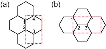
Figure 7: (Color online) Doubled unit cells of graphene for the (a) armchair and (b) zigzag construction. The bases are indexed in the same order as the $4\times 4$ matrix representation of $H(\vec{k})$ in the text.

Because $r\neq 0$, this equation is a fourth-order polynomial of $r$ and has four solutions. Equation (5) is invariant under the operations $r\rightarrow\frac{1}{r}$ and $\frac{1}{r}\rightarrow r$. If $r_{s}$ is a solution to Eq. (5), then $r_{s}^{*},\frac{1}{r_{s}}$, and $\frac{1}{r_{s}^{*}}$ are also solutions of the secular equation. If the solution has a nonzero $\kappa$ ($=Im\ k_{x}$), then the four solutions correspond to left- and right-decaying states and their time-reversal pairs. The existence condition of the complex band can be derived if $\kappa$ is set to zero.

To visualize the energy-dependent decay length, consider a special case of the band edge: $k_{y}=\frac{1}{2}G_{\|}=\frac{\pi}{3a}$. In this case, if we put $s=-1$, the equation becomes

$$\left\{r+\frac{1}{r}+3-\left(\frac{E}{t}\right)^{2}\right\}^{2}=0.$$ (6)

The solution of equation (6) is

$$\sqrt{3}k_{x}a=\begin{cases}\pm\pi\pm i\cosh^{-1}\left\{\frac{3}{2}-\frac{1}{2}\left(\frac{E}{t}\right)^{2}\right\},&E^{2}\leq t^{2}\\ \pm\cos^{-1}\left\{-\frac{3}{2}+\frac{1}{2}\left(\frac{E}{t}\right)^{2}\right\},&t^{2}<E^{2}\leq 5t^{2}\\ \pm i\cosh^{-1}\left\{-\frac{3}{2}+\frac{1}{2}\left(\frac{E}{t}\right)^{2}\right\},&5t^{2}<E^{2}\end{cases}$$

and numerical solutions are plotted for the case of $k_{y}=0,\frac{\pi}{6a}$, and $\frac{\pi}{3a}$ in Fig. 4(a), (b), and (c), respectively.

In the same manner, for graphene in the zigzag direction, the Hamiltonian $H(k_{x},k_{y})$ is given by

$$\begin{bmatrix}0&t(1+e^{i\vec{k}\cdot\vec{R_{y}}})&0&te^{-i\vec{k}\cdot\vec{R_{x}}}\\ t(1+e^{-i\vec{k}\cdot\vec{R_{y}}})&0&t&0\\ 0&t&0&t(1+e^{-i\vec{k}\cdot\vec{R_{y}}})\\ te^{i\vec{k}\cdot\vec{R_{x}}}&0&t(1+e^{i\vec{k}\cdot\vec{R_{y}}})&0\end{bmatrix},$$

where $\vec{k}=(k_{x},k_{y})$, $\vec{R_{x}}=(3a,0)$, and $\vec{R_{y}}=(0,\sqrt{3}a)$. The order of the basis ($i$ = 1, 2, 3, and 4) is shown in Fig. 7(b). If we define $r\equiv e^{i\vec{k}\cdot\vec{R_{x}}}$ and $s\equiv e^{i\vec{k}\cdot\vec{R_{y}}}$, then secular equation for a given $E$ and $k_{y}$ can be written as follows:

$$0 = \frac{det(E-H)}{t^{4}}$$ (7)

$$= 5-\{2+2Re(s)\}\left(r+\frac{1}{r}\right)+4\{Re(s)\}^{2}$$

$$+ \left\{8-4\left(\frac{E}{t}\right)^{2}\right\}Re(s)+\left(\frac{E}{t}\right)^{4}-6\left(\frac{E}{t}\right)^{2}.$$

With respect to the variable $r$, this equation has two solutions connected by an inverse relation. From this equation we can calculate the decay length of the edge states of the GNR. Because the edge state of a zigzag-edged GNR is a zero-energy mode, the $k_{y}$-dependence of the decay length is obtained by solving the following equation,

$$\{2+2Re(s)\}\left(r+\frac{1}{r}\right)=\{2+2Re(s)\}^{2}+1.$$ (8)

The solution of equation (8) is $k_{x}a=\pm\frac{i}{3}\ln\left\{4\cos^{2}\left(\frac{\sqrt{3}k_{y}a}{2}\right)\right\}$, and numerical solutions are plotted for the cases of $k_{y}=0,\frac{2\pi}{3\sqrt{3}a}$, and $\frac{\pi}{\sqrt{3}a}$ in Fig. 4(d), (e) and (f), respectively.

References

- (1) K. S. Novoselov, A. K. Geim, S. V. Morozov, D. Jiang, Y. Zhang, S. V. Dubonos, I. V. Grigorieva and A. A. Firsov, Science 306, 666 (2004).
- (2) S. Ryu and Y. Hatsugai, Phys. Rev. Lett. 89, 077002 (2002).
- (3) P. Koskinen, S. Malola, and H. Häkkinen, Phys. Rev. Lett. 101, 115502 (2008).
- (4) N. W. Ashcroft and N. D. Mermin, Solid State Physics (Saunders College, 1976).
- (5) W. Kohn, Phys. Rev. 116, 809 (1959).
- (6) V. Heine, Proc. Phys. Soc. London 81, 300 (1962).
- (7) V. Heine, Phys. Rev. 138, A1689 (1965).
- (8) Y.-C. Chang, Phys. Rev. B 25, 605 (1982).
- (9) J. P. Perdew, K. Burke, and M. Ernzerhof, Phys. Rev. Lett. 77, 3865 (1996).
- (10) G. Kresse and D. Joubert, Phys. Rev. B 59, 1758 (1999).
- (11) G. Kresse and J. Furthmüller, Phys. Rev. B 54, 11169 (1996).
- (12) The package can be obtained from the web page (http://www.quantum-espresso.org/).
- (13) D. Vanderbilt, Phys. Rev. B. 41, 7892 (1990).
- (14) A. M. Rappe, K. M. Rabe, E. Kaxiras, and J. D. Joannopoulos, Phys. Rev. B 41, 1227 (1990).
- (15) F. D. Murnaghan, Proc. Natl. Acad. Sci. USA 30, 244 (1944).
- (16) F. Birch, Phys. Rev. 71, 809 (1947).
- (17) H. J. Monkhorst and J. D. Pack, Phys. Rev. B 13, 5188 (1976).
- (18) G.-D. Lee, C. Z. Wang, E. Yoon, N.-M. Hwang, and K. M. Ho, Phys. Rev. B 81, 195419 (2010).
- (19) K. W. Kolasinski, Surface Science (Wiley, 2008).
- (20) C. Park, H. Yang, A. J. Maynec, G. Dujardin, S. Seo, Y. Kuk, J. Ihm and G. Kim, Proc. Natl. Acad. Sci. USA 108, 18622 (2009).
- (21) N. Marzari and D. Vanderbilt, Phys. Rev. B i56, 12847 (1997).
- (22) W. Li and R. Tao, J. Phys. Soc. Jpn. 81, 024704 (2012).
- (23) H. J. Choi, J. Ihm, S. G. Louie, and M. L. Cohen, Phys. Rev. Lett. 84, 2917 (2000).
- (24) G. Kim, B. W. Jeong and J. Ihm, Appl. Phys. Lett. 88, 193107 (2006).
- (25) D. L. Smith and C. Mailhiot, Rev. Mod. Phys. 62, 173 (1990).
- (26) Y.-W. Son, M. L. Cohen and S. G. Louie, Phys. Rev. Lett. 97, 216803 (2006).
- (27) Y.-W. Son, S. G. Louie and M. Cohne, Nature 444, 347 (2006).