CMB likelihood approximation for banded probability distributions

Abstract

We investigate sets of random variables that can be arranged sequentially such that a given variable only depends conditionally on its immediate predecessor. For such sets, we show that the full joint probability distribution may be expressed exclusively in terms of uni- and bivariate marginals. Under the assumption that the CMB power spectrum likelihood only exhibits correlations within a banded multipole range, $\Delta\ell$, we apply this expression to two outstanding problems in CMB likelihood analysis. First, we derive a statistically well-defined hybrid likelihood estimator, merging two independent (e.g., low- and high-$\ell$) likelihoods into a single expression that properly accounts for correlations between the two. Applying this expression to the WMAP likelihood, we verify that the effect of correlations on cosmological parameters in the transition region is negligible in terms of cosmological parameters for WMAP; the largest relative shift seen for any parameter is $0.06\sigma$. However, because this may not hold for other experimental setups (e.g., for different instrumental noise properties or analysis masks), but must rather be verified on a case-by-case basis, we recommend our new hybridization scheme for future experiments for statistical self-consistency reasons. Second, we use the same expression to improve the convergence rate of the Blackwell-Rao likelihood estimator, reducing the required number of Monte Carlo samples by several orders of magnitude, and thereby extend it to high-$\ell$ applications.

1. Introduction

The cosmic microwave background (CMB) radiation is one of the most pristine sources of information about the early Universe available to us. Since its discovery in 1964 (Penzias & Wilson, 1965), the amount of information available to us about the CMB has increased at a rapid pace through series of ground-based, sub-orbital and satellite experiments. The recently released Planck temperature sky maps (Planck I, 2013) is just the latest example of how the present challenge in the field of cosmology is one of overabundance rather than shortage of data.

To extract cosmological parameters from these ever growing data sets requires increasingly sophisticated and efficient algorithms, both due to larger data volumes and to more stringent requirements to statistical precision. For example, the COBE-DMR sky maps published twenty years ago (Smoot et al., 1992) comprised $\mathcal{O}(10^{4})$ pixels, and could be analyzed using exact brute-force likelihood techniques (e.g., Górski, 1994), with a computational scaling of $\mathcal{O}(N_{\textrm{pix}}^{3})$. The WMAP sky maps published ten years ago comprised $\mathcal{O}(10^{7})$ pixels (Bennett et al., 2003a), at which point faster and approximate methods had to be used for parameter estimation (Hivon et al., 2002; Verde et al., 2003). However, for WMAP the error budget was still dominated by cosmic variance on large angular scales and instrumental noise on small angular scales, and confusion with Galactic and extra-Galactic emission was minimal, allowing for very simple component separation methods (Bennett et al., 2003b; Hinshaw et al., 2003). For Planck, the total number of data points in nine frequency bands is $\mathcal{O}(3\cdot 10^{8})$, and instrumental noise never dominates the uncertainties at any angular scales, as small-scale astrophysical confusion becomes important at multipoles $\ell\gtrsim 1500$ (Planck XII, 2013). As a result, an unprecendented study of all important sources of uncertainty, including instrumental, systematic and astrophysical, was required for Planck to reach its ambitious goals (Planck XV, 2013).

With the advent of these massive mega-pixel data sets, a number different analysis strategies have been developed to robustly extract cosmological parameters with acceptable computational cost. As of today, the preferred option for full-sky high-resolution experiments such as Planck and WMAP is to divide the analysis into two separate components according to large and small angular scales, and merge the two at the likelihood level. On large angular scales, they use a Gibbs sampling based (Jewell et al., 2004; Wandelt et al., 2004; Eriksen et al., 2004, 2007) Blackwell-Rao estimator (Chu et al., 2005) that takes into account the full non-Gaussian structure of the true CMB likelihood, while on small angular scales, they use faster approaches (e.g., Hivon et al., 2002; Rocha et al., 2011; Planck XV, 2013) coupled to an analytic multivariate Gaussian (and/or log-normal) likelihood approximation. The computational cost of this hybrid approach is dominated by spherical harmonics transforms, and therefore scales as $\mathcal{O}(N_{\textrm{pix}}^{3/2})$, which is acceptable even for large data sets. However, there is an unsolved problem associated with this hybrid approach, and that is how to merge the two likelihood components into a single all-scale expression; correlations between the smallest scales in the large-scale likelihood and the largest scales in the small-scale likelihood should in principle be accounted for. As of today, no fully satisfactory solution to this exists in the CMB literature, though various approaches were explored during the Planck analysis.

Having a computational scaling of $\mathcal{O}(N_{\textrm{pix}}^{3/2})$, the Gibbs sampling approach could in principle be employed for all angular scales, thus eliminating the need for any hybrid approximation. Unfortunately, in practice this method is in its current implementation limited to low angular scales for two reasons: First, joint CMB analysis and component separation is currently implemented in terms of pixel-based fits of physical foreground models, requiring all frequency bands to have the same angular resolution, dictated by the coarsest resolution in a given data set. Second, although the computational scaling for the Gibbs sampler is acceptable, the prefactor is high. The 2013 Planck likelihood employed 100 000 Gibbs samples in order to achieve robust Blackwell-Rao convergence, and each of those samples required $\sim$2000 Conjugate Gradient iterations (and twice as many spherical harmonic transforms) to converge, for a total cost of 500 000 CPU hours. Naively scaling this to full Planck resolution suggest a final cost of $\mathcal{O}(10^{8})$ CPU hours.

The main result of the present paper is a statistically well motivated block factorization of the CMB power spectrum likelihood that is applicable to several of these problems. Specifically, we show that for sets of random variables that can be arranged sequentially in such a way that all correlations have a finite range within the sequence, the full joint probability distribution may be written in terms of lower-dimensional marginals. The arch-typical example of such a distribution is a multivariate Gaussian with a strictly banded covariance matrix, and we therefore call the general (non-Gaussian but conditionally limited) case also “banded”. With this statistical identity ready at hand, we first suggest a statistically well-motivated likelihood hybridization scheme that takes properly into account correlations between the low- and high-$\ell$ regimes, and, second, we show how the convergence rate of the Blackwell-Rao estimator can be improved by factorizing the full high-dimensional multivariate posterior into a set of lower-dimensional distributions, each of which converges much faster than the full distribution. This approach differs from the direct Gaussianization technique proposed by Rudjord et al. (2009) in that the underlying probabilistic structure (e.g., shapes of marginal and $N$-point correlations) is conserved; in principle, the only modification to the full likelihood enforced by our new approach is that assumed negligible correlations are explicitly set to zero.

2. Factorizing the CMB likelihood

2.1. Factorization of banded probability distributions

We begin with a general joint probability density $P(\{\theta\})=P(\theta_{1},\theta_{2},\theta_{3},\dots,\theta_{n})$ for a set of random variables, $\theta_{k}$, with $k=1,2,3,\dots,n$. We choose one specific sequential ordering of these variables (out of all the possible orderings), and use the definition of a conditional to write the joint distribution as a product of univariate conditionals,

$$P(\{\theta\})= \quad P(\theta_{1},\theta_{2},\theta_{3},\dots,\theta_{n})$$

$$= \quad P(\theta_{1}|\theta_{2},\theta_{3},\dots,\theta_{n})$$

$$\cdot P(\theta_{2}|\theta_{3},\dots\theta_{n})\cdots$$

$$\cdot P(\theta_{n-1}|\theta_{n})\cdot P(\theta_{n})$$

We then assume that our variables only have a conditional probability dependence on their immediate neighbors in the sequence, i.e., that the probability distribution is tri-diagonally banded,

$$P(\{\theta\})\approx \,P(\theta_{1}|\theta_{2})\cdot\,P(\theta_{2}|\theta_{3})\cdots\,P(\theta_{n-1}|\theta_{n})\cdot\,P(\theta_{n})$$

$$= \,\frac{P(\theta_{1},\theta_{2})}{P(\theta_{2})}\cdot\frac{P(\theta_{2},\theta_{3})}{P(\theta_{3})}\cdots\frac{P(\theta_{n-1},\theta_{n})}{P(\theta_{n})}\cdot P(\theta_{n})$$

$$= \,\frac{\prod_{k=1}^{n-1}P(\theta_{k},\theta_{k+1})}{\prod_{k=2}^{n-1}P(\theta_{k})}.$$ (1)

Thus, this simple derivation shows that a strictly (tri-diagonally) banded probability distribution may be factorized recursively into a product of uni- and bivariate marginals.

Before applying this expression to CMB likelihood approximation, we note that even if the joint probability distribution do not have correlations exclusively between neighboring variables, it may still be possible to factorize it, provided at least some correlations may be ignored. For instance, suppose we can ignore all but the nearest two neighbors; in that case, the joint distribution will factorize into a product of uni-, bi- and trivariate marginals.

2.2. Block factorization of the CMB likelihood

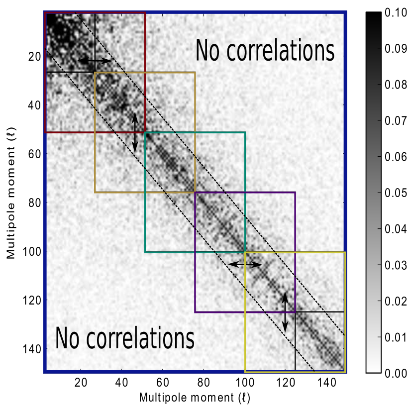
Figure 1.— Angular power spectrum correlation matrix, $M_{\ell\ell^{\prime}}$, for the official Planck low-$\ell$ CMB data set, estimated by Monte Carlo sampling. Note that any two-point correlations are contained within a band of $\Delta\ell\sim 15$, suggesting that the CMB likelihood may be approximated as a banded probability distribution. To factorize the CMB likelihood into lower-dimensional elements, we partition the full multipole range into a set of disjoint blocks such that all non-zero covariance elements are embedded within a tri-diagonal block structure, indicated here by colored squares.

In its most basic representation, a CMB data set, $\mathbf{d}$, may be modelled as

$$\mathbf{d}=\mathbf{s}+\mathbf{n},$$ (2)

where $\mathbf{s}$ is the true sky signal and $\mathbf{n}$ represents instrumental noise. Both the signal and noise are usually assumed to be zero-mean Gaussian variables with covariances $\mathbf{S}$ and $\mathbf{N}$, respectively.

The noise covariance matrix is typically given by external knowledge about the instrumental noise characteristics and the scanning strategy of a given experiment. The signal covariance matrix, on the other hand, is generally unknown, and must be estimated from the data. However, given the fact that we only have one observable sky available, it is impossible to estimate the $N_{\textrm{pix}}^{2}$ elements in $\mathbf{S}$ from the $N_{\textrm{pix}}$ elements in $\mathbf{d}$ without imposing strong priors on its structure. The most commonly accepted prior is simply that the CMB sky is isotropic and homogeneous (e.g., Planck XXIII, 2013). It is therefore convenient to expand $\mathbf{s}$ in spherical harmonics, such that

$$\mathbf{s}(\hat{\mathbf{n}})=\sum_{\ell,m}a_{\ell m}Y_{\ell m}(\hat{\mathbf{n}}),$$ (3)

where $\hat{\mathbf{n}}$ is a unit vector pointing to a given position on the sky, $Y_{\ell m}$ are the spherical harmonics, and $a_{\ell m}$ are the corresponding spherical harmonics coefficients. Then the signal covariance matrix may be written as

$$S_{\ell m,\ell^{\prime}m^{\prime}}=\left<a_{\ell m}a^{*}_{\ell^{\prime}m^{\prime}}\right>\equiv C_{\ell}\delta_{\ell\ell^{\prime}}\delta_{mm^{\prime}},$$ (4)

where $C_{\ell}$ is known as the angular power spectrum.

The main goal of most CMB experiments is precisely to measure the CMB power spectrum, and the most straightforward way to do so is by maximum-likelihood estimation. Since we have assumed that both signal and noise are Gaussian distributed, the CMB power spectrum likelihood simply reads

$$\mathcal{L}(C_{\ell})\equiv P(\mathbf{d}|C_{\ell})\propto\frac{e^{-\frac{1}{2}\mathbf{d}^{t}(\mathbf{S}(C_{\ell})+\mathbf{N})^{-1}\mathbf{d}}}{\sqrt{|\mathbf{S}(C_{\ell})+\mathbf{N}|}},$$ (5)

where $\mathbf{S}=\mathbf{S}(C_{\ell})$ is the covariance matrix given in Equation 4 expressed in pixel domain. Note that $C_{\ell}$ denotes the set of all power spectrum coefficients, and the likelihood therefore spans an $\ell_{\textrm{max}}$-dimensional space.

As already mentioned, brute-force evaluation of Equation 5 scales computationally as $\mathcal{O}(N_{\textrm{pix}}^{3})$, and is therefore feasible only for very low angular resolutions. Much of the CMB analysis literature therefore revolves around finding computationally tractable approximations to this expression.

In order to build up some intuition about the correlation structure of $\mathcal{L}(C_{\ell})$, it is useful to plot the correlation matrix

$$M_{\ell\ell^{\prime}}\equiv\frac{\left<(C_{\ell}-\left<C_{\ell}\right>)(C_{\ell^{\prime}}-\left<C_{\ell^{\prime}}\right>\right>}{\sqrt{\left<(C_{\ell}-\left<C_{\ell}\right>)^{2}\right>\left<(C_{\ell^{\prime}}-\left<C_{\ell^{\prime}}\right>)^{2}\right>}}.$$ (6)

Figure 1 shows this matrix for the official Planck low-$\ell$ CMB data, as evaluated from $200,000$ Monte Carlo samples generated with a CMB Gibbs sampler (Eriksen et al., 2007). In this case, there are significant correlations between all elements at $\ell\lesssim 20$, while at $\ell\gtrsim 50$ any correlations are well contained inside a band of $\Delta\ell=15$; any correlations beyond $\Delta\ell\gtrsim 30$ are well below 1 %. Higher-order correlations are significantly smaller than these two-point correlations.

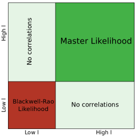
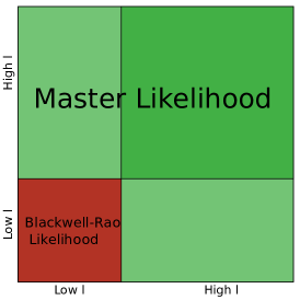
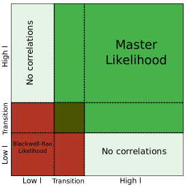
Figure 2.— Schematic overview of the three hybridization schemes discussed in the text. The left panel illustrates a sharp transition between the low- (Blackwell-Rao) and high-$\ell$ (MASTER) likelihood, as currently adopted by Planck. The middle panel illustrates the WMAP approach, which includes the off-diagonal elements between the low- and high-$\ell$ regions in the high-$\ell$ likelihood estimator. The right panel illustrates the new estimator proposed in this paper, in which correlations are accounted for through an transition region that is sufficiently wide to include all non-negligible correlations between the low- and high-$\ell$ regions. To avoid double-counting of the diagonal elements, the total log-likelihood is corrected by the log-likelihood including elements within the transition region only.

For typical sky cuts and instrumental noise characteristics, the basic CMB likelihood can therefore be approximated as a banded probability distribution with a bandwidth of $\Delta\ell\lesssim 15$, and can therefore in principle be factorized by Equation 1. However, as currently written this expression only applies to a strictly tri-diagonal covariance matrix. To circumvent this problem, we therefore introduce an auxiliary block structure that embeds all non-negligible elements within a larger tri-diagonal structure, as illustrated by the colored blocks in Figure 1. That is, we define a set of multipole blocks such that $\theta_{1}=\{C_{\ell_{\textrm{min}}},\ldots,C_{\ell_{1}}\}$, $\theta_{2}=\{C_{\ell_{1}+1},\ldots,C_{\ell_{2}}\}$, …, $\theta_{n}=\{C_{\ell_{n-1}+1},\ldots,C_{\ell_{\textrm{max}}}\}$. Thus, each univariate marginal in Equation 1 is replaced with a multivariate distribution of dimension $\ell_{i}-\ell_{i-1}$, and each bivariate marginal is replaced with a multivariate distribution of dimension $\ell_{i}-\ell_{i-2}$. This block-wise factorization constitutes the main result of this paper, and in the following sections we will apply this to two concrete problems in CMB likelihood estimation.

Table 1Summary of cosmological parameters derived with three different hybridization schemes; the original WMAP approach including off-diagonal elements in the inverse covariance matrix (second column); a sharp transition at $\ell_{\textrm{trans}}=32$ (third column); and the new approach implementing a transition region between $\ell=21$ and 32 (fifth column). The fourth and sixth columns show the relative shifts with respect to the WMAP approach measured in units of $\sigma$.

	Default WMAP	Sharp transition		Transition region
	Constraint	Constraint	Deviation ($\sigma$)	Constraint	Deviation ($\sigma$)
$\Omega_{b}h^{2}$	$0.0225\pm 0.0006$	$0.0225\pm 0.0006$	$0.02$	$0.0225\pm 0.0006$	$0.02$
$\Omega_{m}h^{2}$	$0.111\pm 0.005$	$0.111\pm 0.005$	$0.01$	$0.112\pm 0.006$	$0.05$
$\theta$	$1.039\pm 0.003$	$1.039\pm 0.003$	$0.04$	$1.039\pm 0.003$	$0.05$
$\tau$	$0.088\pm 0.015$	$0.088\pm 0.015$	$0.04$	$0.088\pm 0.015$	$0.05$
$n_{s}$	$0.969\pm 0.013$	$0.969\pm 0.014$	$0.03$	$0.968\pm 0.014$	$0.06$
$\textrm{log}[10^{10}A_{s}]$	$3.08\pm 0.04$	$3.08\pm 0.03$	$0.03$	$3.08\pm 0.04$	$0.05$

Note. — The confidence intervals are 1 $\sigma$, and the best-fit points are the marginalised means of the parameters.

3. Accurate hybrid CMB likelihood estimation

As already mentioned, both Planck and WMAP have adopted so-called ”hybrid” likelihood approximations, combining a Gibbs sampling based Blackwell-Rao estimator at large angular scales with a Gaussian (and/or log-normal) pseduo cross-spectrum approximation at small angular scales. These two components are merged into a single expression at the log-likelihood level. The Planck likelihood simply adds the two log-likelihoods (Planck XV, 2013), adopting a so-called “sharp transition” between the low- and high-$\ell$ regimes, schematically illustrated in the left panel of Figure 2. This is the simplest possible approach, and assumes that any correlations across the transition multipole are negligible. The WMAP likelihood makes a different choice, by including the off-diagonal terms between the low- and high-$\ell$ blocks in the (Gaussian plus log-normal) high-$\ell$ likelihood, as illustrated in the middle panel of Figure 2.

In this section, we introduce a new and statistically better motivated approach than either of two employed by Planck and WMAP, taking advantage of the block factorization derived in Equation 1. The first step in our approach is to partition the full multipole range between $\ell_{\textrm{min}}$ and $\ell_{\textrm{max}}$ into three disjoint regions, $L=\{\ell_{\textrm{min}},\ldots,\ell_{\textrm{low}}\}$, $T=\{\ell_{\textrm{low}}+1,\ldots,\ell_{\textrm{high}}-1\}$ and $H=\{\ell_{\textrm{high}},\ldots,\ell_{\textrm{max}}\}$, corresponding to a low-$\ell$ region, a transition region and a high-$\ell$ region, respectively. The width of the transition region is chosen to be at least as wide as the effective bandwidth of the $C_{\ell}$ covariance matrix (see Figure 1). With this partitioning, we now specialize Equation 1 to the case with $n=3$ regions;

$$\log\mathcal{L}(C_{\ell})=\log\mathcal{L}(L,T)+\log\mathcal{L}(T,H)-\log\mathcal{L}(T).$$ (7)

Note that this approximation is exact under the assumption of vanishing correlations between the low- and high-$\ell$ regions, which can be ensured simply by letting the transition region be sufficiently wide. This estimator is schematically illustrated in the right panel of Figure 2.

Equation 7 has a simple intuitive interpretation: The log-likelihood is simply the sum of a low- and a high-$\ell$ contribution, defined such that they overlap over a sufficiently wide multipole range that all non-negligible correlations are included. However, because the diagonal block in the transition region is included twice, both by the low- and the high-$\ell$ likelihood, one must subtract the corresponding marginal for the transition region once to avoid double-counting (this is also an immediate consequence of equation 1, under the assumption that $p(L|T,H)=p(L|T)=p(L,T)/P(T)$, i.e. the low-$\ell$ region is conditionally independent of the high-$\ell$ region given the transition region). Note that any estimator for the transition likelihood may be used for the correction term, typically by extracting the relevant range from either the low- or the high-$\ell$ likelihoods.

To assess the importance of the specific strategy adopted for hybridization, we modify the (7-year) WMAP likelihood to include each of the three solutions, and derive constraints on the standard $\Lambda$CDM model using WMAP data only. The transition multipole is set to $\ell_{\textrm{trans}}=32$ for the sharp transition case, whereas the transition region is defined as $\ell=\{21,\ldots,32\}$ for the new hybrid scheme. The WMAP Blackwell-Rao estimator is used both for the low-$\ell$ and the transition regions in the latter case. We adopt $\Omega_{b}h^{2},\Omega_{m}h^{2},\theta,\tau,n_{s},$ and $\log(10^{10}A_{s})$ as our primary parameters, and adopt CosmoMC (Lewis & Bridle, 2002) as our MCMC engine. The resulting one-dimensional marginals are shown in Figure 3 for all three cases, and posterior mean summary statistics are given in Table 1.

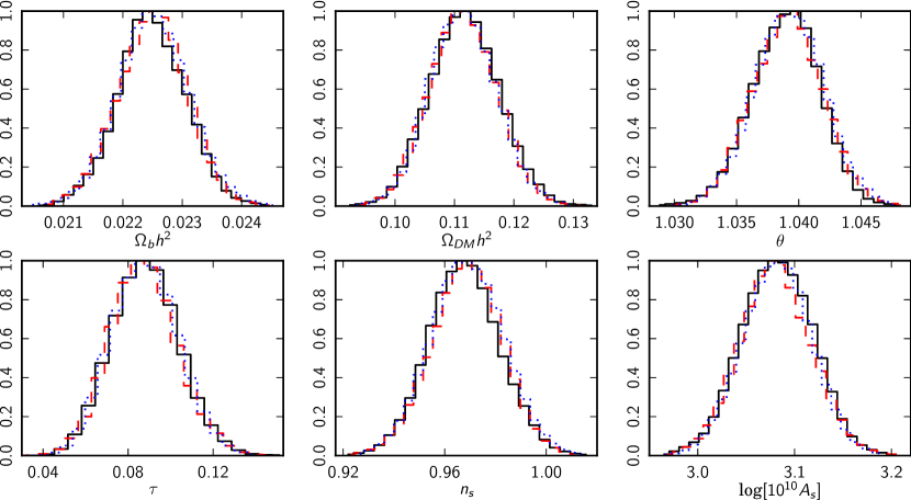
Figure 3.— Comparison of best-fit parameters derived by CosmoMC from WMAP using likelihood approximations based on the new hybrid estimator presented in this paper (solid black line); the WMAP approach including off-diagonal elements in the inverse covariance matrix (dashed red line); and a sharp transition between the low- and high-$\ell$ regions (dotted blue line).

With a largest relative difference between any two cases of $0.06\sigma$, these results demonstrate that the standard six-parameter $\Lambda$CDM model is highly robust with respect to assumptions about the correlations across the transition regime. Similar conclusions were found when performing an identical analysis for the the recently released Planck likelihood (Planck XV, 2013), and this motivated the choice of a sharp transition for that particular implementation. For future experiments and analyses we nevertheless recommend the hybrid approach presented here, for two main reasons. First, our expression provides a statistically well motivated solution whose validity may be monitored directly through the $C_{\ell}$ covariance matrix; without the same level of statistical rigour, detailed simulations are more critical for the other two approaches, and these should in principle be repeated both when the data set or the parametric model is changed. Second, this expression is implementationally trivial once both low- and high-$\ell$ likelihoods are available, and there is therefore no practical reason for not including these correlations, even if their impact may be small.

4. Faster Blackwell-Rao convergence

4.1. Review of the Blackwell-Rao estimator

As mentioned in Section 1, both the Planck and WMAP low-$\ell$ likelihoods (Planck XV, 2013; Hinshaw et al., 2012) employs a specific Blackwell-Rao (BR) estimator to produce an accurate likelihood approximation that accounts for all correlations and non-Gaussian structures (Chu et al., 2005). The main advantages of this estimator are 1) computational speed, 2) implementational simplicity, and 3) support for seamless marginalization over systematic effects and component separation errors through Gibbs sampling (Eriksen et al., 2007).

This estimator may be explained intuitively as follows: Suppose it is possible to construct an experiment that provides a perfect full-sky noiseless image of the CMB sky, $\mathbf{d}=\mathbf{s}$. For that experiment, the only source of uncertainty on $C_{\ell}$ is cosmic variance, and the exact CMB likelihood in Equation 5 reduces to an inverse Gamma distribution,

$$\mathcal{L}_{0}(C_{\ell})\propto\frac{e^{-\frac{1}{2}\mathbf{s}^{t}\mathbf{S}(C_{\ell})^{-1}\mathbf{s}}}{\sqrt{|\mathbf{S}(C_{\ell})|}}\propto\prod_{\ell}\sigma_{\ell}^{-\frac{2\ell-1}{2}}\frac{e^{\frac{2\ell+1}{2}\frac{\sigma_{\ell}}{C_{\ell}}}}{C_{\ell}^{\frac{2\ell+1}{2}}}.$$ (8)

Here we have defined $\sigma_{\ell}\equiv\frac{1}{2\ell+1}\sum_{\ell=-m}^{m}|a_{\ell m}|^{2}$ to be the realization specific power spectrum of $\mathbf{s}$.

However, for any real experiment there are additional sources of uncertainty beyond cosmic variance, for instance from instrumental noise and foreground contamination, and $P(\mathbf{s}|\mathbf{d})$ is no longer a delta function. In order to account for this additional uncertainty, one must weight the ideal likelihood in Equation 8 with respect to $P(\mathbf{s}|\mathbf{d})$,

$$\mathcal{L}_{\textrm{BR}}(C_{\ell})=\int d\mathbf{s}\,\mathcal{L}_{0}(C_{\ell})\,P(\mathbf{s}|\mathbf{d}).$$ (9)

At first glance, this integral appears difficult to evaluate, as it involves millions of degrees of freedom. However, this is precisely where the CMB Gibbs sampler enters the picture. As explained in detail by Jewell et al. (2004); Wandelt et al. (2004); Eriksen et al. (2004, 2007), the output from this algorithm is a set of samples drawn directly from $P(\mathbf{s}|\mathbf{d})$, accounting for both instrumental noise and foreground errors. Thus, the integral can be simply evaluated by Monte Carlo integration as a sum over these samples,

$$\mathcal{L}_{\textrm{BR}}(C_{\ell})\approx\sum_{i=1}^{N_{\textrm{samp}}}\prod_{\ell=\ell_{\textrm{min}}}^{\ell_{\textrm{max}}}{\sigma^{i}_{\ell}}^{\frac{2\ell-1}{2}}\frac{e^{\frac{2\ell+1}{2}\frac{\sigma^{i}_{\ell}}{C_{\ell}}}}{C_{\ell}^{\frac{2\ell+1}{2}}}.$$ (10)

This is the CMB power spectrum Blackwell-Rao estimator, which is guaranteed to converge to the true likelihood in the limit of $N_{\textrm{samp}}\rightarrow\infty$.

4.2. Lifting the “curse of dimensionality”
by block factorization

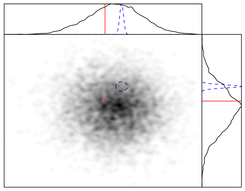
Figure 4.— Illustration of the “curse of dimensionality”. The Blackwell-Rao estimator builds up a smooth histogram from a finite set of Monte Carlo samples by assigning a distribution (or kernel) to each sample. The number of samples required to reach convergence is proportional to the ratio between the volume of the kernel (blue) and the volume of the full distribution (black). If this ratio is $r<1$ in one dimension (top and left panels), it is $r^{2}$ in two dimensions (central panel), and $r^{n}$ in $n$ dimensions. This implies that the number of Monte Carlo samples required to reach convergence for the CMB BR estimator scales exponentially with $\ell_{\textrm{max}}$. The evaluation of the 2-d likelihood at a specific point in parameter space (red cross) will be much more sensitive to the number of samples than the corresponding evaluations in the respective marginalized parameter spaces (red lines).

While the Blackwell-Rao estimator is guaranteed to converge to the correct answer, it is not obvious how fast it does so, as measured in terms of number of samples required for convergence, $N_{\textrm{samp}}$. Further, since the computational cost of a single Gibbs sample is typically on the order of several CPU hours (Eriksen et al., 2004), depending on the angular resolution and/or signal-to-noise ratio of the data set under consideration, it is important to understand this scaling before attempting a full-scale analysis. Indeed, Chu et al. (2005) showed that $N_{\textrm{samp}}$ scales exponentially with $\ell_{\textrm{max}}$, effectively limiting its operational range to $\ell_{\textrm{max}}\approx 50$–70. The main goal of the present section is to improve on this limit, and extend the BR estimator to high $\ell$’s.

To understand the origin of the exponential scaling, we show in Figure 4 a simple two-dimensional Gaussian distribution mapped by a Monte Carlo sampler. The top and left panels show the respective one-dimensional marginals. The Blackwell-Rao estimator establishes a smooth approximation to these distributions by assigning a kernel of finite width to each individual Monte Carlo sample (illustrated by blue contours/Gaussians) before taking the average over all samples. Suppose now that the width of the one-dimensional kernel is 10% of the width of the marginal distribution; in that case, one needs $\sim$10 samples in order to cover the marginal once. In two dimensions, however, one needs $\sim$$10^{2}$ samples to cover the full joint distribution once, since the ratio now is only 10% in each of the two directions. More generally, in $n$ dimensions one would need $\sim$$10^{n}$ samples. This is a variation of the well-known “curse of dimensionality”, which says that the number of points required to cover an $n$-dimensional space scales exponentially with $n$.

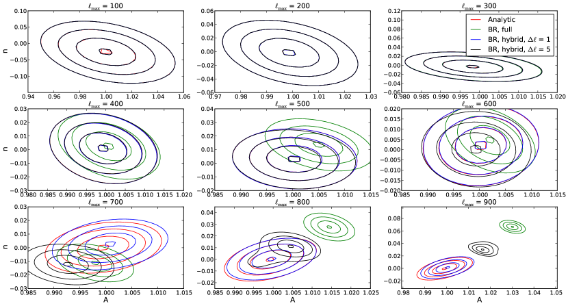
Figure 5.— Comparison of four different methods of evaluating a simple amplitude-tilt likelihood for a full-sky simulation: The analytic case, the full Blackwell-Rao case, and two versions of the hybrid likelihood described in this paper - with $\Delta\ell=1$ and $5$, respectively.

The BR estimator given in Equation 10 converges well up to $\ell\approx 30$ with only a few thousand samples for WMAP (Chu et al., 2005), while for Planck it is found to be robust up to $\ell\approx 70$ with 100 000 samples (Planck XV, 2013). To extend to even higher $\ell$’s by brute force would soon require a prohibitively large number of samples, as the computational cost for the Gibbs sampling step of the latter case is already half a million CPU hours.

Fortunately, the block factorization presented in Section 2 may be used to define an alternative and computationally much cheaper algorithm:

1. Partition the full $\ell_{\textrm{max}}$-dimensional $\mathcal{L}(C_{\ell})$ into a sequence of lower-dimensional blocks, $r_{k}$, for instance of width $\Delta\ell$.

2. Use the standard BR estimator to estimate the marginal likelihood for each block and each neighboring set of two blocks.

3. Merge these block marginals into a single all-$\ell$ estimator through the block factorization in Equation 1.

Thus, our new likelihood approximation can be written succinctly on the following form,

$$\mathcal{L}(C_{\ell})\approx\frac{\prod_{k=1}^{n-1}\mathcal{L}_{\textrm{BR}}(r_{k},r_{k+1})}{\prod_{k=2}^{n-2}\mathcal{L}_{\textrm{BR}}(r_{k})}.$$ (11)

Note that all the likelihood evaluations on the right side of this expression involve a maximum of $2\Delta\ell-1$ dimensions, as opposed to $\ell_{\mathrm{max}}-\ell_{\mathrm{min}}+1$ for the full joint BR estimator, effectively lifting the curse of dimensionality.

4.3. Accuracy and convergence

4.3.1 Methodology

Before the block factorized BR estimator can be used for real analysis, it is necessary to assess its accuracy and convergence properties. To this aim, we analyze two different simulations with the above machinery, adopting the convergence analysis methodology of Chu et al. (2005), but implementing a few minor changes to improve the reliability of the convergence statistics. Monte Carlo samples are produced with Commander (Eriksen et al., 2004, 2007).

The first simulation consists of a full-sky high-resolution ($N_{\textrm{side}}=512$, $\ell_{\textrm{max}}=1024$, 14’ Gaussian beam) data set with uniform noise (65 $\mu\textrm{K}$ RMS per pixel). The main advantage of this case is that the $C_{\ell}$ likelihood (Equation 5) factorizes in $\ell$, and can be evaluated analytically,

$$\mathcal{L}_{\textrm{ideal}}(C_{\ell})\propto\prod_{\ell}\frac{e^{-\frac{2\ell+1}{2}\frac{\hat{\sigma}_{\ell}}{(C_{\ell}+N_{\ell})}}}{(C_{\ell}+N_{\ell})^{\frac{2\ell+1}{2}}},$$ (12)

where $\hat{\sigma}_{\ell}$ is the angular power spectrum of the noisy sky map, and $N_{\ell}$ is the ensemble averaged noise power spectrum. The second simulation consists of a low-resolution ($N_{\textrm{side}}=32$, $\ell_{\textrm{max}}=95$, $4^{\circ}$ FWHM Gaussian beam) data set with the WMAP KQ85 sky cut imposed, removing 25 % of the sky. White noise of 5 $\mu\textrm{K}$ RMS is added to each pixel, resulting in a signal-to-noise of unity at $\ell\approx 70$. The main purpose of this simulation is to study the effect of correlations between different multipoles arising from the sky cut through comparison with brute-force pixel-space likelihood evaluation. However, because of the brute-force evaluations, this case is necessarily limited to low angular resolution.

The CMB signal is drawn from a Gaussian distribution with a covariance given by the best-fit WMAP $\Lambda$CDM power spectrum, $C_{\ell}^{\mathrm{ref}}$ (Hinshaw et al., 2012). In each case, we fit a two-parameter amplitude-tilt ($A$–$n$) model on the form

$$C_{\ell}(A,n)=A\,\left(\frac{\ell}{\ell_{0}}\right)^{n}\,C_{\ell}^{\mathrm{ref}},$$ (13)

where $\ell_{0}=\ell_{\textrm{max}}/2$, simply by mapping out $\mathcal{L}(A,n)$ over a two-dimensional grid. For $\ell_{\mathrm{min}}=2$, this choice of pivot multipole ensures a low degree of correlation between $A$ and $n$.

To assess both convergence and accuracy, we adopt the following measure of difference between two likelihoods, $\mathcal{L}_{1}$ and $\mathcal{L}_{2}$ (Chu et al., 2005),

$$q=\int\left|\mathcal{L}_{1}(A,n)-\mathcal{L}_{2}(A,n)\right|\,dA\,dn.$$ (14)

One can show that if $\mathcal{L}_{1}$ and $\mathcal{L}_{2}$ are two bivariate Gaussian distributions with the same covariance matrix, $\mathbf{\Sigma}$, but different means, $\vec{\mu}_{1}$ and $\vec{\mu}_{2}$, then

$$q=\Phi\left(\frac{1}{2\sqrt{2}}\sqrt{(\vec{\mu}_{1}-\vec{\mu}_{2})\mathbf{\Sigma}^{-1}(\vec{\mu}_{1}-\vec{\mu}_{2})}\right),$$ (15)

where $\Phi$ is the cumulative standard normal distribution function. From this, one finds that a $0.1\sigma$ shift in a Gaussian distribution corresponds to $q\sim 0.05$. In the following, we therefore define two distributions to agree if $q<0.05$.

For the accuracy assessment, we simply compare the block factorized BR likelihood with the exact case. Convergence assessment, however, is done by drawing two disjoint sample subsets from the full set of available Monte Carlo samples, compute the BR estimator from each subset, and compare the resulting likelihoods. We then increase the number of samples in the two subsets, $N_{\textrm{samp}}$, until $q$ is consistently lower than 0.05 even when adding 100 additional samples; the latter criterion is imposed in order to avoid chance agreement. Finally, we repeat this calculation a certain number of times with different sample subsets (but drawn from the same full sample set), and report the median of the resulting values of $N_{\textrm{samp}}$ as the final estimate of the number of samples required for convergence.

4.3.2 Results

Figure 5 shows $\mathcal{L}(A,n)$ evaluated from the high-resolution full-sky simulation for nine different values of $\ell_{\textrm{max}}$ with four different likelihood expressions; analytic, standard BR, and two variations of the block-factorized BR estimator. A total of $N_{\textrm{samp}}=28,000$ samples are included in the two latter, a choice that is set to highlight the fundamental difference between the various cases. In particular, since there are no correlations between any multipoles in this case, all four approaches are in principle exact, and the only difference among the four cases are their relative convergence rates.

For $\ell_{\textrm{max}}\leq 300$, we see that all four estimator agree to very high accuracy. However, from $\ell_{\textrm{max}}\geq 400$ the full-range BR likelihood starts to diverge. At $\ell_{\textrm{max}}=900$, it is separated from the analytic result by more than $15\sigma$. In this case, the sum in Equation 10 is strongly dominated by the one sample that happens to have the lowest power spectrum scatter about some best-fit mode, and the resulting distribution is simply an imprint of the cosmic variance kernel (Equation 8) for that sample.

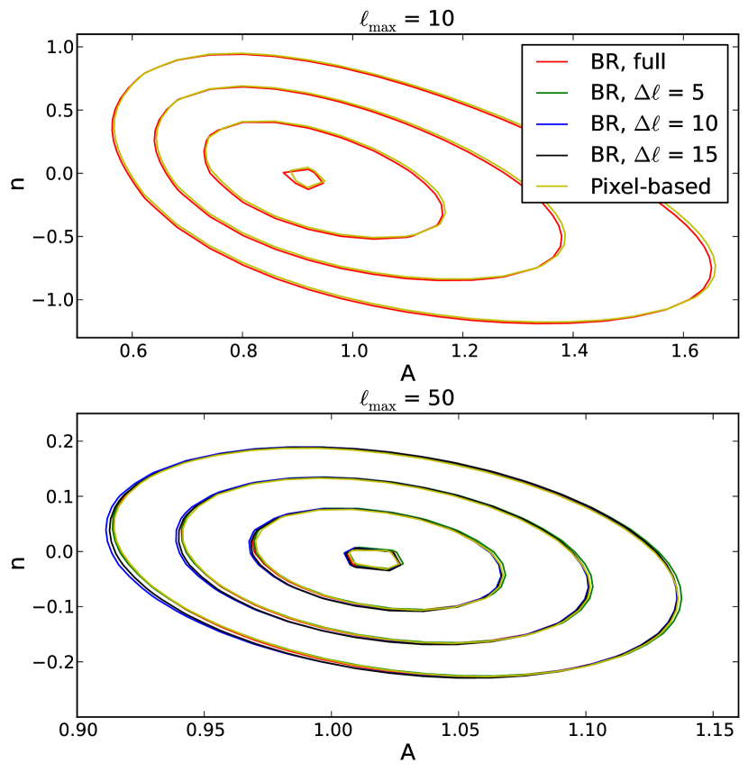
Figure 6.— Comparison of five different methods of evaluating a simple amplitude-tilt likelihood for a cut-sky simulation: The pixel-based case, the full Blackwell-Rao case, and three versions of the hybrid likelihood described in this paper - with $\Delta\ell=5$, $10$, and $15$, respectively.

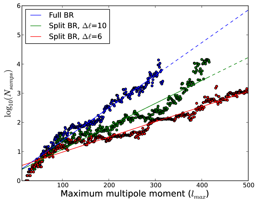
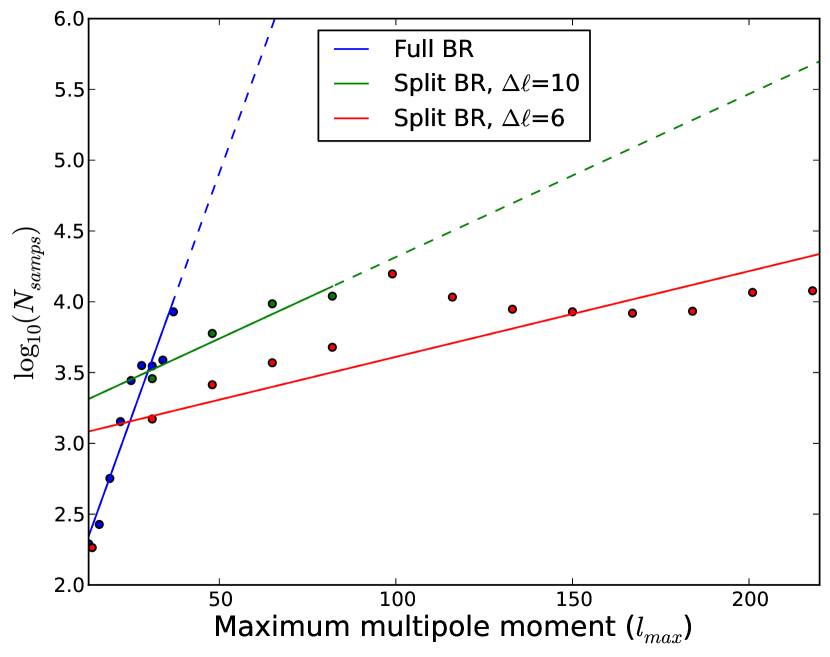
Figure 7.— Convergence analysis for the split Blackwell-Rao estimator, with convergence defined in sec. 4.3. The samples come from running Commander on a full-sky simulation. We show the median of the number of samples needed for convergence for a given $\ell_{\mathrm{max}}$, along with the best-fit regression line in $\log_{10}$-space. The median is computed from 10 (top) and 1024 (bottom) runs where the samples are scrambled between each run. The regression lines are dotted when they extend past the available data points. The high number of runs per data point for the bottom plot is also the reason for the more sparse sampling - each data point represented a very high computational cost, and so the number of data points were reduced.

The block factorized BR estimators remain valid to higher $\ell_{\textrm{max}}$, demonstrating how the “curse of dimensionality” is lifted by breaking the full parameter space into smaller regions that are easier to handle. In particular, the case with $\Delta\ell=1$ agrees with the analytic case even at $\ell_{\textrm{max}}=900$ to $\sim$$0.3\sigma$.

In Figure 6 we show similar results for the low-resolution simulation for which 25 % of the sky is removed by masking, but this time comparing with the brute-force pixel-based likelihood estimator, and this time using $N_{\textrm{samp}}=60,000$ samples. Again, we see that all cases agree to better than $0.1\sigma$, even for the factorized BR estimator with $\Delta\ell=5$, demonstrating the accuracy of both the full and the factorized BR estimators, even with very small block sizes and for the fairly large WMAP mask.

Next, in the top panel of Figure 7 we plot the number of samples required for convergence according to the above criterion for the high-resolution full-sky simulation described above, and in the bottom panel we show the same, but after applying the WMAP mask, in order to introduce a realistic multipole correlation structure. The upper vertical limit in these plots is set by the finite number of samples included in the analysis.

In all cases we see the same qualitative behaviour: Reducing the dimensionality of the BR estimator through block factorization greatly improves the convergence rate by reducing the required number of samples by orders of magnitude at high $\ell$’s. For instance, for the full-sky case and with a block size of $\Delta\ell=6$, only $10^{3}$ samples are required in order to reach convergence up to $\ell_{\textrm{max}}=500$, whereas the full BR estimator would require $10^{6}$. For the 25 % WMAP mask, about $10^{4}$ samples are required for $\ell_{\textrm{max}}=200$, while it is difficult to establish any sensible estimate for the full BR estimator in this case. (Note that the high-$\ell$ projection for the latter case, marked by a dashed line, is based on linear extrapolation from a few low-$\ell$ points, since convergence was not reached at all within the current sample set at higher multipoles. This projection is therefore associated with a very large systematic uncertainty.)

5. Conclusions

The main result presented in this paper is a statistically well motivated block factorization of the CMB power spectrum likelihood. Because the spherical harmonics are nearly orthogonal over the large sky coverages achieved by current CMB satellite experiments such as Planck and WMAP, any correlations between different $C_{\ell}$s are localized in multipole space. Under the assumption that these probabilistic dependencies have a strictly finite range, the full CMB likelihood may be reduced into a product of lower-dimensional marginals.

We have applied this result to two outstanding problems in CMB analysis. First, we use this expression to derive a well-motivated hybrid CMB likelihood estimator, merging an exact low-$\ell$ component with an approximate high-$\ell$ component, that accounts for correlations between the two regions. Although a detailed analysis of the WMAP likelihood shows that these correlations are negligible for the WMAP sky cut and the six-parameter $\Lambda$CDM model, we nevertheless recommend this new estimator for future experiments and analyses, both because its implementation is trivial, and because it provides additional safety when analyzing non-standard models.

Second, we have shown how the same expression may be used to accelerate the convergence rate of the Blackwell-Rao CMB likelihood estimator by orders of magnitude at high $\ell$s. This is achieved by factorizing the full parameter space into subspaces that each individually converge faster, and then merging these sub-blocks into a full-range estimator at the likelihood level using the block factorization formula.

It should be noted that these results rely directly on the assumption of vanishing long-range correlations. While this assumption holds to a very high accuracy for the basic CMB signal plus noise data model, it is in general not valid when including systematic effects in the analysis. Perhaps the two most important examples are correlated beam uncertainties and unresolved extra-Galactic point sources, each of which extend through all $\ell$’s (e.g., Planck XV, 2013). Fortunately, these long-range degrees of freedom may be modelled in terms of a small number of power spectrum templates, each with an unknown amplitude. One can therefore marginalize over these by sampling the unknown amplitudes as nuiscance parameters, similar to what was done for high-$\ell$ astrophysical parameters in the 2013 Planck likelihood (Planck XV, 2013).

Finally, we note that the block factorization presented in Section 2 is a completely general statistical result that holds exactly for any banded probability distribution, and we therefore expect it to also find applications outside the CMB field.

References

- Bennett et al. (2003a) Bennett, C. L., Halpern, M., Hinshaw, G., et al. 2003a, ApJS, 148, 1
- Bennett et al. (2003b) Bennett, C. L., Hill, R. S., Hinshaw, G., et al. 2003b, ApJS, 148, 97
- Chu et al. (2005) Chu, M., Eriksen, H. K., Knox, L., et al. 2005, Phys. Rev. D, 71, 103002
- Eriksen et al. (2004) Eriksen, H. K., O’Dwyer, I. J., Jewell, J. B., et al. 2004, ApJS, 155, 227
- Eriksen et al. (2007) Eriksen, H. K., Jewell, J. B., Dickinson, C., Banday, A. J., Górski, K. M., & Lawrence, C. R. 2007, ApJ, 676, 19
- Górski (1994) Górski, K. M. 1994, ApJ, 430, L85
- Górski et al. (2005) Górski, K. M., Hivon, E., Banday, A. J.,Wandelt, B. D., Hansen, F. K., Reinecke, M., Bartelman, M. 2005, ApJ, 622, 759
- Hinshaw et al. (2003) Hinshaw, G., Spergel, D. N., Verde, L., et al. 2003, ApJS, 148, 135
- Hinshaw et al. (2012) Hinshaw, G., Larson, D., Komatsu, E., et al. 2012, arXiv:1212.5226
- Hivon et al. (2002) Hivon, E., Górski, K. M., Netterfield, C. B., et al. 2002, ApJ, 567, 2
- Jarosik et al. (2011) Jarosik, N., Bennett, C. L., Dunkley, J., et al. 2011, ApJS, 192, 14
- Jewell et al. (2004) Jewell, J., Levin, S., & Anderson, C. H. 2004, ApJ, 609, 1
- Lewis & Bridle (2002) Lewis, A., & Bridle, S. 2002, Phys. Rev. D, 66, 103511
- Penzias & Wilson (1965) Penzias, A. A., & Wilson, R. W. 1965, ApJ, 142, 419
- Planck I (2013) Planck Collaboration I 2013, [1303.5062]
- Planck XII (2013) Planck Collaboration XII 2013, [1303.5072]
- Planck XV (2013) Planck Collaboration XV 2013, [1303.XXXX]
- Planck XVI (2013) Planck Collaboration XVI 2013, [1303.5076]
- Planck XXIII (2013) Planck Collaboration XXIII 2013, [1303.5083]
- Planck XXIV (2013) Planck Collaboration XXIV 2013, [1303.5084]
- Rocha et al. (2011) Rocha, G., Contaldi, C. R., Bond, J. R., & Górski, K. M. 2011, MNRAS, 414, 823
- Rudjord et al. (2009) Rudjord, Ø., Groeneboom, N. E., Eriksen, H. K., et al. 2009, ApJ, 692, 1669
- Smoot et al. (1992) Smoot, G. F., Bennett, C. L., Kogut, A., et al. 1992, ApJ, 396, L1
- Verde et al. (2003) Verde, L., Peiris, H. V., Spergel, D. N., et al. 2003, ApJS, 148, 195
- Wandelt et al. (2004) Wandelt, B. D., Larson, D. L., & Lakshminarayanan, A. 2004, Phys. Rev. D, 70, 083511