Counter effects of meridional flows and magnetic fields in stationary axisymmetric self-gravitating barotropes under the ideal MHD approximation: Clear examples — toroidal configurations

Abstract

We obtain the general forms for the current density and the vorticity from the integrability conditions of the basic equations which govern the stationary states of axisymmetric magnetized self-gravitating barotropic objects with meridional flows under the ideal MHD approximation. As seen from the stationary condition equations for such bodies, the presence of the meridional flows and that of the poloidal magnetic fields act oppositely on the internal structures.

The different actions of these two physical quantities, the meridional flows and the poloidal magnetic fields, could be clearly seen through stationary structures of the toroidal gaseous configurations around central point masses in the framework of Newtonian gravity because the effects of the two physical quantities can be seen in an amplified way for toroidal systems compared to those for spheroidal stars. The meridional flows make the structures more compact, i.e. the widths of toroids thinner, while the poloidal magnetic fields are apt to elongate the density contours in a certain direction depending on the situation. Therefore the simultaneous presence of the internal flows and the magnetic fields would work as if there were no such different actions within and around the stationary gaseous objects such as axisymmetric magnetized toroids with internal motions around central compact objects under the ideal MHD approximation, although these two quantities might exist in real systems.

1 Introductory analysis and motivation

1.1 Theoretical treatment of stationary states of axisymmetric magnetized self-gravitating barotropes under the ideal MHD approximation

In this paper, we give new expressions for the current density and the vorticity vector inside the stationary and axisymmetric magnetized self-gravitating barotropes with internal gaseous motions under the ideal magnetohydrodynamics (MHD) approximation. Although stationary states of the magnetized self-gravitating barotropes without internal flows have been investigated in many old papers (e.g., Chandrasekhar & Fermi 1953; Lüst & Schlüter 1954; Ferraro 1954; Gjellestad 1954; Roberts 1955; Chandrasekhar 1956a; Chandrasekhar 1956b; Chandrasekhar & Prendergast 1956; Prendergast 1956; Sykes 1957; Woltjer 1959a; Woltjer 1959b; Woltjer 1960; Ostriker & Hartwick 1968) and in recent papers (e.g., Tomimura & Eriguchi 2005; Yoshida & Eriguchi 2006; Yoshida et al. 2006; Otani et al. 2009; Fujisawa et al. 2012), the effects of the internal flows on structures of magnetized self-gravitating barotropes have barely studied so far.

Dynamic equilibrium equations for stationary states of magnetized self-gravitating bodies with internal flows are given by

$${1\over\rho}\nabla p=-\nabla\phi_{g}-\nabla\phi_{c}-{1\over 2}\nabla|\mbox{\boldmath$v$}|^{2}+\mbox{\boldmath$v$}\times\mbox{\boldmath$\omega$}+{1\over c\rho}\mbox{\boldmath$j$}\times\mbox{\boldmath$B$}\ ,$$ (1)

where $\rho$, $p$, $\phi_{g}$, $\phi_{c}$, $v$, $\omega$, $c$, $j$, and $B$ are the density, the pressure, the gravitational potential of the gaseous body, the gravitational potential of external objects, the fluid velocity, the vorticity vector, the speed of light, the current density, and the magnetic field, respectively. In this study, the gravitational potential of external objects is assumed to be given by

$$\phi_{c}=-{GM_{c}\over r}\,,$$ (2)

where $M_{c}$, $G$, and $r$ denote the mass of the central external object, the gravitational constant, and the distance from the central object, respectively. Using the expressions for the current density and the vorticity vector inside the stationary, axisymmetric and infinitely conducting barotropes (for details, see Appendix A), we may simplify the forth term in the right-hand side of Eq. (1) as

$$\mbox{\boldmath$v$}\times\mbox{\boldmath$\omega$}=\left\{\begin{array}[]{ll}\Omega(\Psi)\nabla(Rv_{\varphi})+\displaystyle{1\over 4\pi c\rho}\displaystyle{dQ(\Psi)\over d\Psi}\mbox{\boldmath$B$}\times\mbox{\boldmath$\omega$}\ ,&(\mbox{for $\mbox{\boldmath$B$}\neq 0,\mbox{\boldmath$v$}_{p}\neq 0$})\\ \nu(Q)\nabla Q\ ,&(\mbox{for $\mbox{\boldmath$B$}=0,\mbox{\boldmath$v$}_{p}\neq 0$})\\ {1\over 2}\nabla(R^{2}\Omega^{2}(R))+R\Omega^{2}(R)\mbox{\boldmath$e$}_{R}\ ,&(\mbox{for $\mbox{\boldmath$B$}=0,\mbox{\boldmath$v$}_{p}=0$})\end{array}\right.$$ (6)

where $\Psi$ and $Q$ are the flux and stream functions, respectively (see Eqs. (39) and (40)), $\Omega$ and $\nu$ are arbitrary functions of the given argument, and $R$ and $\mbox{\boldmath$e$}_{R}$ are the radial coordinate and base vector for the cylindrical coordinate with respect to the symmetry axis, respectively. We describe the details of these arbitrary functions in Appendix A and Appendix B. Here, $\mbox{\boldmath$v$}_{p}$ and $v_{\varphi}$ stand for the poloidal velocity and the toroidal velocity, given by

$$\mbox{\boldmath$v$}_{p}={1\over 4\pi\rho}\nabla Q\times\nabla\varphi\,,$$ (7)

$$v_{\varphi}=R\Omega+\displaystyle{1\over 4\pi c\rho}\displaystyle{dQ(\Psi)\over d\Psi}B_{\varphi}\,,$$ (8)

with $\varphi$ and $B_{\varphi}$ being the azimuthal angle and the toroidal magnetic field, respectively. The stream function $Q$ is a function of the flux function $\Psi$ if and only if $\mbox{\boldmath$B$}\neq 0$ and $\mbox{\boldmath$v$}_{p}\neq 0$. Thus, equi-stream function surfaces are similar to equi-magnetic flux function surfaces if $\mbox{\boldmath$B$}\neq 0$ and $\mbox{\boldmath$v$}_{p}\neq 0$. Similarly, the Lorentz force term appearing in the fifth term in the right-hand side of Eq. (1) may be rewritten as

$${1\over c\rho}\mbox{\boldmath$j$}\times\mbox{\boldmath$B$}=\left\{\begin{array}[]{ll}\nabla(\Omega(\Psi))Rv_{\varphi}+\mu(\Psi)\nabla\Psi+\displaystyle{1\over 4\pi c\rho}\displaystyle{dQ(\Psi)\over d\Psi}\mbox{\boldmath$\omega$}\times\mbox{\boldmath$B$}\ ,&(\mbox{for $\mbox{\boldmath$B$}\neq 0$})\\ 0\ ,&(\mbox{for $\mbox{\boldmath$B$}=0$})\\ \end{array}\right.$$ (11)

where $\mu(\Psi)$ is an arbitrary function. From Eqs. (1)–(11), we obtain Bernoulli’s equations for the present situation:

$$\int{dp\over\rho}=\left\{\begin{array}[]{l}-\phi_{g}+\displaystyle{GM_{c}\over r}-{1\over 2}(|\mbox{\boldmath$v$}_{p}|^{2}+v_{\varphi}^{2})+Rv_{\varphi}\Omega(\Psi)+\int^{\Psi}\mu(\Psi)d\Psi+C\ ,\\ \qquad(\mbox{for $\mbox{\boldmath$B$}\neq 0$})\\ -\phi_{g}+\displaystyle{GM_{c}\over r}-{1\over 2}(|\mbox{\boldmath$v$}_{p}|^{2}+v_{\varphi}^{2})+\int^{Q}\nu(Q)dQ+C\ ,\\ \qquad(\mbox{for $\mbox{\boldmath$B$}=0,\mbox{\boldmath$v$}_{p}\neq 0$})\\ -\phi_{g}+\displaystyle{GM_{c}\over r}+\int^{R}R\Omega^{2}dR+C\ ,\\ \qquad(\mbox{for $\mbox{\boldmath$B$}=0,\mbox{\boldmath$v$}_{p}=0$})\\ \end{array}\right.$$ (18)

where $C$ is an integration constant. It should be emphasized that these three expressions cannot be united to a single expression as can be understood from Eqs. (6) and (11). Note that in this study, we do not consider the case of $\mbox{\boldmath$B$}_{p}=0$ and $B_{\varphi}\neq 0$, for which Bernoulli’s equations differ from Eq. (18).

By comparing Bernoulli’s equation for the case of $\mbox{\boldmath$B$}=0$ and $\mbox{\boldmath$v$}_{p}=0$ with that for the case of $\mbox{\boldmath$B$}=0$ and $\mbox{\boldmath$v$}_{p}\neq 0$, we may expect that the presence of the meridional flows tends to decrease the volume occupied by the fluid. This is because the kinetic energy of the meridional flow contributes to the fluid as positive ram pressures (dynamic pressure), which result in reducing the fluid pressure and consequently decreasing the density of stationary fluid objects. In contrast to the effect of the meridional flow, for magnetized equilibrium configurations with $\mbox{\boldmath$v$}_{p}=0$ whose magnetic fields are generated by positive toroidal currents, the poloidal magnetic field is apt to expand the fluid region to the direction perpendicular to the symmetry axis like the centrifugal force (see, e.g. old papers Ferraro 1954; Gjellestad 1954; Roberts 1955; and recent papers Tomimura & Eriguchi 2005; Yoshida & Eriguchi 2006; Yoshida et al. 2006; Fujisawa et al. 2012). Therefore, simultaneous presence of the meridional flows and the poloidal magnetic fields could result in almost no changes in the matter distributions. So far, such effects have not been investigated because stationary states of axisymmetric magnetized barotropes with meridional flows have not been obtained. Thus it is one of the purposes in this study to show the above statements could be proved to hold in some numerical examples.

1.2 Toroids: Best astrophysical systems in which both meridional flows and magnetic fields would work simultaneously but differently

In order to show clearly the oppositely working effects of the above mentioned two quantities, meridional flows and poloidal magnetic fields, we will show numerical results of stationary configurations of axisymmetric magnetized self-gravitating toroidal barotropes with meridional flows which locate around central point masses in the framework of Newtonian gravity under the ideal MHD approximation. For toroidal configurations, matter distribution changes in wider space would be expected compared to size changes of spheroidal objects because toroids could change their shapes to two opposite directions, i.e. to the outside direction and to the inside direction of the toroids. Thus we will solve stationary states of axisymmetric magnetized barotropic toroids with meridional flows under the ideal MHD approximation and clarify the oppositely working effects explicitly in this study.

Concerning self-gravitating toroidal configurations or disks, we need to take recent results of fully general relativistic (GR) numerical simulations into account. These simulations show that a few-solar-mass black hole and a highly dense toroid whose maximum density can reach $10^{10}$ - $10^{11}\mathrm{g/cm}^{3}$ around the black hole could be formed after merging of binary neutron stars (Shibata & Uryū 2000; Shibata et al. 2003; Shibata et al. 2005; Kiuchi et al. 2009; Hotokezaka et al. 2011), after merging of a neutron star and a black hole in binary systems (Shibata & Uryū 2006;Shibata & Uryu 2007; Shibata & Taniguchi 2008; Kyutoku et al. 2010; Kyutoku et al. 2011) or after collapsing of a supermassive rotating star (Shibata 2000; Shibata & Shapiro 2002; Shibata 2003; Sekiguchi & Shibata 2004; Sekiguchi & Shibata 2007; Sekiguchi & Shibata 2011). Therefore, dense toroids and central compact objects could be formed after collapsing or merging of compact objects. Similar kinds of systems with magnetic fields have also been investigated by several groups (e.g. Narayan et al. 2001; Shibata & Sekiguchi 2005; Duez et al. 2006; Shibata et al. 2007). Although, in order to understand the origin and dynamical formation processes of these systems, we must take into account many realistic physics and compute stationary configurations with magnetic fields in GR, nobody has yet succeeded in solving stationary states both with poloidal and toroidal magnetic fields in GR at present. Therefore, we explore such stationary states of axisymmetric magnetized barotropic systems in the framework of Newtonian gravity. Although there were many papers to obtain magnetized stationary states of disks/toroids only with poloidal magnetic fields (e.g. Bisnovatyi-Kogan & Blinnikov 1972; Bisnovatyi-Kogan & Seidov 1985; Baureis et al. 1989; Li & Shu 1996) and disks/toroids only with toroidal magnetic fields inside the disks/toroids (e.g. Okada et al. 1989; Banerjee et al. 1995; Ghanbari & Abbassi 2004), no solutions both with poloidal and toroidal components of magnetic fields have been obtained yet. This is because it has been difficult to solve the Grad-Shafranov equation as well as the equations of motion consistently by some means. Concerning this type of systems, the most general formulation was derived by Lovelace et al. (1986) systematically. However, Lovelace et al. (1986) computed solutions only with poloidal magnetic fields for non-self-gravitating disks.

Recently, Otani et al. (2009) have obtained magnetized self-gravitating equilibrium states both with poloidal and toroidal magnetic fields self-consistently in the framework of Newtonian gravity. Their method is based on Tomimura & Eriguchi (2005). In this study we have extended the method employed in Otani et al. (2009) to the most general configurations for the stationary states of axisymmetric magnetized barotropic toroids with meridional flows under the ideal MHD approximation and obtained sequences of stationary states. Comparing these results with those of non-magnetized toroids without meridional flows (e.g. Ostriker 1964;Wong 1974), with those of magnetized toroids without meridional flows (e.g. Otani et al. 2009) or with those of non-magnetized toroids with meridional flows (e.g. Eriguchi et al. 1986), we will be able to clearly see the effect of the presence of both physical quantities, i.e. meridional flows and magnetic fields as explained in the previous subsection.

2 Brief description of the problem

In this study, as mentioned, we investigate stationary configurations of axisymmetric magnetized polytropic toroids with internal fluid motions. We consider inviscid and infinitely conductive toroids with equatorial symmetry located around central point masses in the framework of Newtonian gravity. Since a similar problem, but without meridional flows, was already treated by Otani et al. (2009) and our strategy is basically the same as theirs, we briefly summarize the basic equations, boundary conditions, and solving scheme. We describe the details of physical quantities and dimensionless forms in Appendix C and the numerical scheme in Appendix D.

Continuity and pressure balance equations for stationary states are respectively given by

$$\nabla\cdot(\rho\mbox{\boldmath$v$})=0\,,$$ (19)

$$\frac{1}{\rho}\nabla p=-\nabla\phi_{g}+\nabla\left(\frac{GM_{c}}{r}\right)-\frac{1}{2}\nabla|\mbox{\boldmath$v$}^{2}|+\mbox{\boldmath$v$}\times\mbox{\boldmath$\omega$}+\frac{1}{\rho}\left(\frac{\mbox{\boldmath$j$}}{c}\times\mbox{\boldmath$B$}\right)\,.$$ (20)

The Poisson equation for $\phi_{g}$ is

$$\Delta\phi_{g}=4\pi G\rho\,.$$ (21)

We make use of the polytropic equation of state

$$p=K_{0}\rho^{1+\frac{1}{N}}\,,$$ (22)

where $K_{0}$ and $N$ are a constant and the polytropic index, respectively.

Maxwell equations for stationary electromagnetic fields are

$$\nabla\cdot\mbox{\boldmath$B$} = 0\,,$$ (23)

$$\nabla\times\mbox{\boldmath$E$} = 0\,,$$ (24)

$$\nabla\times\mbox{\boldmath$B$} = 4\pi\frac{\mbox{\boldmath$j$}}{c}\,,$$ (25)

where $E$ is the electric field, which is determined by the perfect conductivity condition

$$\mbox{\boldmath$E$}+\frac{\mbox{\boldmath$v$}}{c}\times\mbox{\boldmath$B$}=0\,.$$ (26)

The magnetic flux function $\Psi$ is, in terms of the azimuthal component of the vector potential $A_{\varphi}$, defined by

$$\Psi=RA_{\varphi}\ .$$ (27)

From the azimuthal component of the Maxwell equation (25), we obtain

$$R\dfrac{\partial\Psi}{\partial R}\left(\frac{1}{R}\dfrac{\partial\Psi}{\partial R}\right)+\dfrac{\partial^{2}\Psi}{\partial z^{2}}=-4\pi R\frac{j_{\varphi}}{c}\ ,$$ (28)

where the cylindrical coordinates $(R,\varphi,z)$ have been used. This equation is equivalent to the so called Grad-Shafranov equation for this problem, but we treat the right-hand side of Eq. (28) as the source term of the differential operator in the left-hand side of Eq. (28) even though $j_{\varphi}$ includes the term proportional to the left-hand side of Eq. (28) if $\mbox{\boldmath$v$}_{p}\neq 0$. Explicit expression for $j_{\varphi}$ is given in Eq. (45). In order to solve Eq. (28) numerically, it is useful to transform Eq. (28) into

$$\Delta(A_{\varphi}\sin\varphi)=-4\pi\frac{j_{\varphi}}{c}\sin\varphi\,,$$ (29)

where $\Delta$ denotes the Laplacian (see, e.g., Tomimura & Eriguchi 2005 and Otani et al. 2009).

Because isolated mass and current densities are considered in this study, boundary conditions at infinity for the gravitational potential $\phi_{g}$ and the vector potential $A_{\varphi}$ are respectively given by

$$\phi_{g}={\cal O}\left(\frac{1}{r}\right)\,,\hskip 10.0ptA_{\varphi}={\cal O}\left(\frac{1}{r}\right)\,.$$ (30)

Solutions for the present problem are obtained by solving the pressure balance equation and the two Poisson equations for $\phi_{g}$ and $A_{\varphi}\sin\varphi$ with the boundary condition (30). In order to impose the boundary condition (30) automatically, in this study, the two Poisson equations (21) and (29) are converted into the two integral equations, given by

$$\phi_{g} = -G\int\frac{\rho(\mbox{\boldmath$r$}^{\prime})}{|\mbox{\boldmath$r$}-\mbox{\boldmath$r$}^{\prime}|}\,d^{3}\mbox{\boldmath$r$}^{\prime}\ ,$$ (31)

$$A_{\varphi}(r,\theta)\sin\varphi = \frac{1}{c}\int\frac{j_{\varphi}(\mbox{\boldmath$r$}^{\prime})}{|\mbox{\boldmath$r$}-\mbox{\boldmath$r$}^{\prime}|}\sin\varphi^{\prime}\,d^{3}\mbox{\boldmath$r$}^{\prime}\ .$$ (32)

Integrating Eq. (20), we obtain Eq. (18). Eqs. (18), (31), and (32) are the master equations for the present problem, which are solved with a variant of the numerical scheme used by Otani et al. (2009) (for details, see Appendix D).

In general, the toroid cannot approach indefinitely to the central object because gravitational effects of the central object can unboundedly increase as the distance from the central object to the toroid decreases and any forces counteracting the gravity cannot stanch the matter flow shedding from the inner edge of the toroid if their distance is shorter than some critical value. In the present numerical scheme to obtain magnetized toroids, the distance from the central object to the inner edge of the toroid (or the width of the toroid) is characterized by a dimensionless parameter $q$, defined by

$$q\equiv\frac{R_{\rm{inner}}}{R_{\rm{outer}}},$$ (33)

where $R_{\rm{inner}}$ and $R_{\rm{outer}}$ are the shortest and the longest distances from the symmetry axis to the toroid, respectively. In terms of $q$, this disappearance property of the equilibrium sates describes as the existence of $q_{c}$ such that there is no stationary solution of the toroid for $q<q_{\rm c}$. Note that the value of $q_{c}$ depends on what parameters characterizing equilibrium sequences keep constant when the value of $q$ changes. Following Otani et al. (2009), we call equilibrium solutions characterized by $q=q_{c}$ the critical configuration or the critical state. The distance from the symmetry axis to the inner edge of the toroid for the critical configuration is named the critical distance. In this study, we focus only on the critical configurations.

Otani et al. (2009) investigated the critical configuration for the magnetized toroids without meridional flows and found the following properties. (i) The critical configuration features cusp-like structures at the inner edge of the toroids. (ii) The critical configuration rotates very slowly. This implies that the critical toroids are mainly sustained by the balance among the magnetic forces, the gravity of the central objects and the pressure gradients. (iii) The critical distances are almost independent of the mass ratio of the toroids to the central objects. (iv) The critical distances are much larger than $6GM_{c}/c^{2}$, the radius of the innermost stable circular orbit for the Schwarzschild black hole with the gravitational mass $M_{c}$. This means that making use of Newtonian gravity is reasonable to investigate structures of the toroids considered in Otani et al. (2009).

3 Numerical results

Following Otani et al. (2009), we consider two polytropic indices $N=1.5$ and $N=3$ only in the present study. As for the arbitrary functions, which need to be specified to obtain particular solutions, we employ the same functional forms as those used in Yoshida et al. (2006) and Otani et al. (2009) except for the toroidal current function $\mu$. For the toroidal current function $\mu$, we choose the same functional form as that used in Fujisawa et al. (2012) in order for the inner edge of the toroid to have stronger magnetic fields. As for the stream function $Q^{\prime}$, which does not appear in Otani et al. (2009), a similar functional form to that of the poloidal current function $\kappa$ is employed. Details of the functional forms of the arbitrary functions are collected in Appendix A.2.

As mentioned before, recent numerical simulations performed with numerical relativity show that geometrically thick toroids rotating around black holes form after mergers of neutron star binaries, mergers of black hole-neutron star binaries, or collapses of supermassive rotating stars (e.g. Sekiguchi & Shibata 2007; Sekiguchi & Shibata 2011). Typical values of physical quantities of such black hole-toroid systems are given by $M_{t}=1.0\times 10^{-1}M_{\odot}$, $M_{c}=5.0M_{\odot}$ ($M_{t}/M_{c}=2.0\times 10^{-2}$), and $\rho_{\rm{c}}=1.0\times 10^{11}\rm{g/cm^{3}}$, where $M_{t}$ and $\rho_{\rm{c}}$ are the mass and the maximum density of the toroid, respectively. Since these black hole-toroid systems are of large significance in high energy astrophysics, we focus on the models characterized by the mass ratio $M_{t}/M_{c}=2.0\times 10^{-2}$ and use these values of the mass of the central object and the maximum density of the toroid to estimate values of other physical quantities with physical dimension, e.g. $|\mbox{\boldmath$B$}|$ and $R_{inner}$.

To check numerical accuracies of the stationary configurations obtained in this study, we estimate values of a virial relation, which vanishes for exact stationary solutions:

$${\rm VC}=\left|\frac{2T+W+3\Pi+\mathfrak{M}}{W}\right|\ ,$$ (34)

where $T,W,\Pi$, and $\mathfrak{M}$ are the kinetic energy, the gravitational energy, the volume integral of the pressure and the magnetic energy, respectively (for details, see Appendix C). As shown later, all the stationary configurations obtained in this study are within acceptable accuracy (for details, see Appendix E).

3.1 Widening of the widths of toroids: Effect of the localized poloidal magnetic fields

$m$	$q_{c}$	$\hat{\mu}_{0}$	$r_{e}$(cm)	$|\hat{W}|$	$\mathfrak{M}/|W|$	$U/|W|$	VC
				$N=1.5$
0.5	0.680	6.960E+00	2.984E+07	2.573E-02	6.509E-01	1.164E-01	2.763E-05
0.3	0.650	4.700E+00	2.791E+07	3.893E-02	6.421E-01	1.193E-01	2.713E-05
0.0	0.598	2.984E+00	2.518E+07	7.401E-02	6.272E-01	1.243E-01	2.610E-05
-0.1	0.578	2.661E+00	2.432E+07	9.226E-02	6.218E-01	1.261E-01	2.575E-05
-0.3	0.533	2.238E+00	2.264E+07	1.449E-01	6.100E-01	1.300E-01	2.525E-05
-0.5	0.481	2.033E+00	2.105E+07	2.312E-01	5.966E-01	1.345E-01	2.444E-05
-0.7	0.419	1.996E+00	1.954E+07	3.754E-01	5.812E-01	1.396E-01	2.381E-05
-0.9	0.344	2.117E+00	1.812E+07	6.201E-01	5.631E-01	1.456E-01	2.329E-05
-1.1	0.252	2.408E+00	1.683E+07	1.036E+00	5.415E-01	1.528E-01	2.274E-05
-1.4	0.067	2.956E+00	1.564E+07	1.923E+00	5.111E-01	1.630E-01	2.471E-05
				$N=3$
0.5	0.720	1.159E+01	4.653E+07	1.747E-03	6.910E-01	1.030E-01	6.433E-05
0.3	0.687	6.031E+00	4.243E+07	3.080E-03	6.807E-01	1.065E-01	6.073E-05
0.0	0.628	2.742E+00	3.656E+07	7.732E-03	6.639E-01	1.121E-01	5.472E-05
-0.1	0.605	2.227E+00	3.473E+07	1.064E-02	6.578E-01	1.141E-01	5.279E-05
-0.3	0.554	1.600E+00	3.129E+07	2.044E-02	6.446E-01	1.185E-01	4.880E-05
-0.5	0.495	1.289E+00	2.814E+07	3.993E-02	6.297E-01	1.234E-01	4.470E-05
-0.7	0.425	1.164E+00	2.529E+07	7.927E-02	6.127E-01	1.291E-01	4.064E-05
-0.9	0.342	1.173E+00	2.274E+07	1.593E-01	5.926E-01	1.358E-01	3.644E-05
-1.1	0.242	1.298E+00	2.057E+07	3.195E-01	5.678E-01	1.441E-01	3.224E-05
-1.4	0.057	1.467E+00	1.901E+07	6.864E-01	5.261E-01	1.580E-01	2.944E-05

Table 1: Physical quantities for the critical configurations with $\hat{Q}_{0}=0.0$ (no meridional flow), $\hat{\Omega}_{0}=0.0$ (no rotation) and $\hat{\kappa}_{0}=4.5$.

Figure 1: The density contours on the meridional cross section for four critical configurations with different values of $m$. From left to right, the density contours correspond to the toroids with $m=-1.4$, $m=-0.7$, $m=-0.1$, and $m=0.5$, respectively. Values of the other parameters are $N=3$, $\hat{Q}_{0}=0$, $\hat{\Omega}_{0}=0$, and $\hat{\kappa}_{0}=4.5$. The tear-shaped closure curves with a cusp-like structure indicate the surfaces of the toroids. The density difference between two adjacent contours is one-tenth of the maximum density. It is observed that the width of the toroid on the equator becomes wider as values of $m$ decrease.

Figure 2: Top panel: The poloidal magnetic fields on the meridional plane for the $N=3$ toroids with $m=-1.4$ (solid curves) and $m=0.5$ (dashed curves). Values of the other model parameters are the same as those of the models given in Fig. 1. The tear-shaped closure curves with a cusp-like structure indicate the surfaces of the toroids. Middle left and bottom left panels: $\log_{10}|\mbox{\boldmath$B$}|$ on the equator for two critical configurations with $m=-1.4$ (middle) and $m=0.5$ (bottom), given as functions of $R/r_{e}$. The horizontal axises range from $R_{inner}/r_{e}(=q_{c})$ to $R_{outer}/r_{e}(=1)$. Middle right and bottom right panels: $-\hat{M_{c}}/4\pi\hat{r}$ (thick dashed curve), $\hat{\phi}_{g}$ (thin dashed curve), $-\int\hat{\mu}(\hat{\Psi})\,d\hat{\hat{\Psi}}-\hat{C}$ (dotted curve), and sum of these three potentials (solid curve) on the equator for the critical configurations with $m=-1.4$ (middle) and $m=0.5$ (bottom), given as functions of $R/r_{e}$. The horizontal axises range from $R_{inner}/r_{e}(=q_{c})$ to $R_{outer}/r_{e}(=1)$.

The counter effects of the meridional flows against the magnetic forces on structures of magnetized toroids would be clearly seen for toroids with rather widened shapes due to poloidal magnetic fields. Thus, in this subsection, we will try to compute magnetized toroids with highly localized poloidal magnetic fields because such equilibrium configurations could be toroids with a rather small value of $q$, i.e. the width of toroids on the equatorial plane being rather wide (see e.g. Fujisawa et al. 2012).

To investigate effects of the localized poloidal magnetic fields on the toroid structures, no fluid flow inside the toroid is considered here. Thus, values of the parameters $\hat{Q}_{0}$, $\hat{\Omega}_{0}^{2}$, $\alpha$, and $d$ are taken to be $\hat{Q}_{0}=0$, $\hat{\Omega}_{0}^{2}=0$, $\alpha=0$, and $d=0$ (for details, see Appendix A.2). As for $\hat{\kappa}_{0}$, following Otani et al. (2009), we take $\hat{\kappa}_{0}=4.5$. Since there are no rotation and no meridional flows, the toroids are in stationary states by the balance among the gravitational force of the central object, the Lorentz force and the gas pressure gradient. If there could be very strong poloidal magnetic fields near the central objects, stronger gravitational forces of the central objects could be balanced by the strong magnetic forces near the central objects. For such situations the toroids could be elongated toward the central objects and have wider widths.

Fujisawa et al. (2012) showed that the poloidal magnetic field distributions substantially depend on the parameter $m$ in the arbitrary function $\mu(\Psi)$ for magnetized stars. In particular, they found that negative values of $m$ result in concentration of the poloidal magnetic fields near the symmetry axis of magnetized stars. Thus, it is expected that we may obtain toroids in which poloidal magnetic fields are concentrated near the inner edge of the toroids by choosing an appropriate value of $m$.

We show our numerical results for critical configurations of $N=1.5$ and $N=3$ polytropic sequences in Table 1 and density contours on the meridional cross section of $N=3$ polytropes with $m=-1.4$, $m=-0.7$, $m=-0.1$ and $m=0.5$ in Fig. 1. As seen from these table and figure, the critical distance decreases as the value of $m$ decreases. The density distribution of the $m=-1.4$ toroid is stretched toward the central object because of the strong gravity of the central object. In addition to this, the cusp-like shape at the inner edge of the toroids becomes ’sharper’ as the value of $m$ becomes smaller. We find the same tendency for the $N=1.5$ polytropes.

The top panel of Fig. 2 shows the structures of the magnetic fields on the meridional plane for the $N=3$ critical configurations with $m=-1.4$ (solid curves) and $m=0.5$ (dashed curves). In this figure, the surfaces of the toroids are indicated by the tear-shaped closure curves. The structures of the magnetic fields for the model with $m=-1.4$ are remarkably different from those for the model with $m=0.5$. The shapes of the contours of the magnetic flux function for the toroid with $m=0.5$ look nearly circle, but those for the toroid with $m=-1.4$ deform oblately. Moreover, the magnetic field lines are more densely distributed near the inner edge region of the toroid for the toroid with $m=-1.4$ compared to those for the toroid with $m=0.5$. In other words, the magnetic fields are highly localized toward the central object for the toroid with $m=-1.4$ compared to those of the toroid with $m=0.5$.

The panels in the middle left and the bottom left of Fig. 2 show distributions of $\log_{10}|\mbox{\boldmath$B$}|$ on the equatorial plane, and the panels in the middle right and the bottom right of Fig. 2 show values of each term in the right-hand side of the first line of Eq. (18) on the equatorial plane. Note that the horizontal axises of these figures range from $R_{inner}/r_{e}(=q_{c})$ to $R_{outer}/r_{e}(=1)$. As seen from the middle left and the bottom left panels of Fig. 2, the distributions of the magnetic fields are significantly different for the two equilibrium configurations. The ring of maximum magnetic field strength locates near the inner edge of the toroid for the model with $m=-1.4$, while it locates near the central region of the meridional cross section of the toroid for the model with $m=0.5$. The toroids with $m=-1.4$ can sustain highly localized and strong magnetic fields in the nearer region from the central object compared to the toroids with $m=0.5$ and can extend themselves toward the central object although the gravitational force of the central object is much stronger there. This implies that the toroids with $m=-1.4$ can produce strong magnetic force near their inner edge, which is balanced against the gravitational force of the central compact object as shown later.

In the middle right and the bottom right panels of Fig. 2, the gravitational potential of the central object, $-\hat{M}_{c}/4\pi\hat{r}$ (thick dashed curve), the gravitational potential of the toroids, $\hat{\phi}_{g}$ (thin dashed curve), the magnetic potential (Fujisawa et al. 2012), $-\int\hat{\mu}\,d\hat{\Psi}-\hat{C}$ (dotted curve) and the sum of all the potentials (thick solid curve) are shown as functions of $R/r_{e}$. Here, physical quantities with $(\ \hat{}\ )$ are dimensionless quantities defined in Appendix C.2. From these figures, it is clearly seen that the magnetic force is the primary agent supporting the toroid against the gravitational force of the central object. The gradient of the gravitational potential of the central object for the toroid with $m=-1.4$ is steeper than that for the toroid with $m=0.5$ because the $m=-1.4$ toroid is located closer to the central object than the $m=0.5$ toroid. The magnetic potentials behave very differently for these two equilibrium configurations with different values of $m$. For the $m=0.5$ toroid, the magnetic potential curve has a substantial local minimum at $R/r_{e}\sim 0.9$. For the $m=-1.4$ toroid, however, the magnetic potential curve is shallower and extends within a broader region and its slope is steepest near the inner edge of the toroid. As a result, the strong magnetic fields can exist near the inner edge region of the toroid and their magnetic force supports the toroid against the gravitational force of the central compact object. In this way, the $m=-1.4$ toroid can be in a stationary state even if the gravitational potential becomes much steeper as approaching to the central object.

3.2 Effects of the meridional flows on the magnetized configurations

3.2.1 Basic features of magnetized configurations with meridional flows

Figure 3: The poloidal magnetic fields (left), the meridional flow pattern (right) on the meridional plane for the toroid with $N=1.5$, $\hat{Q}_{0}=20$, $\hat{\Omega}_{0}=1.0\times 10^{-5}$, $m=0$, $q=0.6$, and $\hat{\kappa}_{0}=0.5$. The tear-shaped closure curves with a cusp-like structure indicate the surfaces of the toroids. Length of vectors given in the right panel is not proportional to the speed of the meridional flows and does not have any physical meaning. The bottom panel shows the distribution of the absolute value of the meridional velocity (solid line) and the rotational velocity (dashed line) normalized by the local Kepler velocity on the equatorial plane.

Concerning the parameters which appear in the arbitrary functions, to examine effects of the meridional flow on toroid structures, the following values are chosen in this subsection: $\hat{\kappa}_{0}=0.5$, $\alpha=-0.5$, $d=0.1$, $m=0$ and $\hat{\Omega}_{0}^{2}=1.0\times 10^{-5}$. Note that smaller values of $\hat{\kappa}_{0}$ result in more rapid meridional flows and that this small value of $\hat{\Omega}_{0}$ gives equilibrium configurations with almost no rotation. Parameters for the rotation law are the same as those in Yoshida et al. (2006).

The left panel of Fig. 3 shows contours of the flux function $\Psi$ on the meridional plane for the critical configuration of an $N=1.5$ polytrope with meridional flows. Direction of the fluid velocity on the meridional cross section in the critical configuration is shown in the right panel of Fig. 3. Here, the lengths of the vectors are not proportional to the absolute values of the fluid velocities. Note that the region where the meridional flows are present is only a part of the meridional cross section of the toroid because a particular functional form for $\hat{Q}^{\prime}(\Psi)$ is used to avoid singular behaviors of the meridional flow near the toroid surface (see Appendix A.2). The bottom panel of Fig. 3 displays the velocity distributions normalized by the local Kepler velocity, on the equatorial plane. The solid and dashed curves denote the absolute value of the meridional velocity and the rotational velocity, respectively. As seen from this panel, the rotational velocity is sub-Keplarian, because our rotational parameter $\hat{\Omega}_{0}$ is assumed to be small in this paper. On the other hand, the meridional velocity is slightly faster than the rotational velocity in this parameter region ($\hat{Q}_{0}$ = 20).

As shown in Figs. 2 and 3 (see, also, Table 2 given later), general structures of the toroids and their magnetic fields do not change significantly even when the fluid flows exist on the meridional plane. As argued later, however, the presence of the meridional flows changes the density distributions of the toroids slightly and increases the critical distance a little bit.

3.2.2 Critical distances for magnetized toroids with meridional flows

$\hat{Q}_{0}$	$q_{c}$	$\hat{\mu}_{0}$	$r_{e}$(cm)	$\mathfrak{M}/|W|$	$\Pi/|W|$	$T/|W|$	$T_{p}/|W|$	VC
				$N=1.5$
0	0.597	3.047E+00	2.500E7	6.213E-01	1.262E-01	8.322E-05	0.000E+00	2.656E-05
20	0.600	3.020E+00	2.514E7	6.226E-01	1.255E-01	4.138E-04	3.185E-04	3.032E-05
40	0.605	2.942E+00	2.555E7	6.268E-01	1.235E-01	1.431E-03	1.314E-03	4.271E-05
60	0.615	2.817E+00	2.627E7	6.338E-01	1.199E-01	3.217E-03	3.063E-03	6.505E-05
80	0.629	2.653E+00	2.759E7	6.437E-01	1.148E-01	6.101E-03	5.875E-03	1.595E-04
				$N=3$
0	0.625	2.810E+00	3.551E7	6.583E-01	1.133E-01	9.202E-04	0.000E+00	5.497E-05
20	0.628	2.784E+00	3.570E7	6.598E-01	1.125E-01	1.464E-03	4.866E-04	3.642E-05
40	0.632	2.711E+00	3.622E7	6.639E-01	1.101E-01	2.935E-03	1.842E-03	3.115E-05

Table 2: Physical quantities for the critical configurations with meridional flows. Model parameters are $\hat{\kappa}_{0}=0.5$, $\hat{\Omega}_{0}^{2}=1.0\times 10^{-5}$, and $m=0$.

Figure 4: Top left and middle left panels: Density contours on the meridional cross section for the critical configurations with $\hat{Q}_{0}=0$ (top left) and $\hat{Q}_{0}=80$ (middle left). The heavy curves indicate the surfaces of the toroids. The density difference between two adjacent contours is one-tenth of the maximum density. Top right and middle right panels: $\frac{1}{2}|\hat{\mbox{\boldmath$v$}}^{2}|-\hat{R}\hat{v}_{\varphi}\hat{\Omega}$ (solid curve), $-\hat{M}_{c}/4\pi\hat{r}$ (thick dashed curve), $-\int\hat{\mu}\,d\hat{\Psi}-\hat{C}$ (dotted curve) for the critical configurations with $\hat{Q}_{0}=0$ (top right) and $\hat{Q}_{0}=80$ (middle right), given as functions of $R/r_{e}$. The horizontal axis ranges from $R_{inner}/r_{e}(=q_{c})$ to $R_{outer}/r_{e}(=1)$. Bottom left panel: Densities normalized by $\rho_{c}$ on the equatorial plane for the critical configurations with $\hat{Q}_{0}=0$ (dashed curve) and $\hat{Q}_{0}=80$ (solid curve), given as functions of $R/r_{e}$. The horizontal axises range from $R_{inner}/r_{e}(=q_{c})$ to $R_{outer}/r_{e}(=1)$. Bottom right panel: The dimensionless velocity potential term, $\frac{1}{2}|\hat{\mbox{\boldmath$v$}}^{2}|-\hat{R}\mbox{\boldmath$v$}_{\varphi}\hat{\Omega}$, on the equatorial plane for the the critical configurations with $\hat{Q}_{0}=20$ (solid curve), $\hat{Q}_{0}=40$ (dashed curve) and $\hat{Q}_{0}=80$ (dotted curve), given as functions of $R/r_{e}$. The horizontal axis ranges from $R_{inner}/r_{e}(=q_{c})$ to $R_{outer}/r_{e}(=1)$. The model parameters are $m=0$, $N=1.5$, $\hat{\kappa}_{0}=0.5$, and $\hat{\Omega}_{0}^{2}=1.0\times 10^{-5}$.

In order to study the influence of the meridional flows on the critical distances, we calculate two polytropic sequences ($N=1.5$, $N=3$) by changing the value of $\hat{Q}_{0}$ for the $m=0$ toroidal current function. We fix the other parameters as $\hat{\kappa}_{0}=0.5$, $\alpha=-0.5$, $d=0.1$, and $\hat{\Omega}_{0}^{2}=1.0\times 10^{-5}$ in this subsection. Physical quantities for several models belonging to the two polytropic sequences are tabulated in Table 2. Here, $T_{p}$ denotes the kinetic energy of the meridional flow.

As seen from this table, the energy ratio $T_{p}/|W|$ is much smaller than that of ${\cal M}/|W|$, thus, the kinetic energy of the meridional flow is much smaller than the magnetic energy for the models obtained in the present study. This means that the magnetic forces mainly support the toroids against the gravitational forces of the central objects even when the meridional flow becomes stronger in the present parameter space. The meridional flow cannot change global structures of the toroids and their magnetic fields significantly. However, the energy ratio $T_{p}/|W|$ reaches $\sim 1.0\times 10^{-3}$ when $\hat{Q}_{0}>40$ $(N=1.5)$ and $\hat{Q}_{0}=40$ $(N=3)$. In fact, the critical distance $q_{c}$ increases as $\hat{Q}_{0}$ increases as shown in Table 2. This implies that the toroids tend to shed their mass when the meridional flow becomes stronger. In some sense, therefore, the influence of the meridional flow on the density distribution of the toroids should not be considered to be small. The rotational velocities of these models are also sub-Keplarian. The typical value is about 2 % of the Kepler velocity which is similar to that given in Fig.3. On the other hand, the meridional flow velocity is about several times as large as the rotational velocity. The maximum velocity of the meridional flow for the $\hat{Q}_{0}=80$ model reaches about 10 times as large as that of the rotational velocity.

In order to clarify the effects of the meridional flows, let us investigate the density distributions of toroids and the profiles of potential terms on the equatorial planes for the $N=1.5$ toroids with and without meridional flows. Fig. 4 shows the density contours on the meridional plane (top left and middle left) and the profiles of the potentials on the equator (top right and middle right). Bottom panels of Fig. 4 show the profiles of the density on the equator (left) and the velocity potential term, $\frac{1}{2}|\hat{\mbox{\boldmath$v$}}^{2}|-\hat{R}\hat{v}_{\varphi}\hat{\Omega}$, on the equator (right) as functions of $R/r_{e}$. In the top right panel of Fig. 4, each curve denotes $\frac{1}{2}|\hat{\mbox{\boldmath$v$}}^{2}|-\hat{R}\hat{v}_{\varphi}\hat{\Omega}$ (solid curve), $-\hat{M}_{c}/4\pi\hat{r}$ (thick dashed curve), $\hat{\phi}_{g}$ (thin dashed curve) and $-\int\hat{\mu}d\hat{\Psi}-\hat{C}$ (doted curve). As seen from these profiles, in both the models, the gravitational potentials of the toroid make a tiny contribution to the equilibrium solutions and the balance between the term $-\int\hat{\mu}d\hat{\Psi}-C$ and the gravitational potential of the central object mainly determines the stationary states of the toroid. Taking a detailed look at the middle right panel of Fig. 4, we observe that the potential terms due to the meridional flow and rotation (solid curve) show their maximum value near the radius of $R/r_{e}=0.95$ for the $N=1.5$ models with $\hat{Q}_{0}=80.0$. This very tiny protuberance is considered to appear due to the presence of the meridional flows because as shown in Table 2, the kinetic energy due to rotation is negligible small. More detailed structures of the velocity potential terms can be seen by enlarging these tiny protuberances. The bottom right panel of Fig. 4 shows the profiles of $\frac{1}{2}|\hat{\mbox{\boldmath$v$}}^{2}|-\hat{R}\hat{v}_{\varphi}\hat{\Omega}$ on the equator for $N=1.5$ polytopes with $\hat{Q}_{0}=20$ (solid curve), $\hat{Q}_{0}=40$ (dashed curve) and $\hat{Q}_{0}=80$ (dotted curve). These profiles have double peaks which locate at $\hat{R}\sim 0.85$ and $\hat{R}\sim 0.92$. These double peaks appear from the balance of the density distributions of the toroids and the meridional flows. As we have described in Sec. 1, the presence of the poloidal velocity fields results in reducing the density of toroids (see Eq. (18)). For our numerical examples, the presence of the poloidal velocity fields decreases the density on the equatorial plane around radii of $\hat{R}\sim 0.85$ and $\hat{R}\sim 0.92$, which can be observed in the bottom two panels of Fig.4 (more detailed considerations are given below).

The top left and middle left panels of Fig. 4 show the density distributions of $N=1.5$ toroids with $\hat{Q}_{0}=0.0$ and $\hat{Q}_{0}=80$, respectively. Comparing the top left panel with the middle left panel, we see that the matter distribution of the toroid with $\hat{Q}_{0}=80$ is shifted outward slightly. The bottom left panel of Fig.4 displays the density profiles on the equator for each toroid. The dotted and solid curves denote the density profiles for the models with $\hat{Q}_{0}=0.0$ and $\hat{Q}_{0}=80$, respectively. As seen form this panel, the meridional flows shift the place where the density takes its maximum value outward and make the density gradient around $\hat{R}\sim 0.92$ steeper. This is due to the double peak structure of the velocity potential profiles. The inner peak of this potential affects to decrease the density around $\hat{R}\sim 0.85$ where the density takes the maximum value if there is no meridional flow. On the other hand, the outer peak of this potential also leads to decrease in the density around $\hat{R}\sim 0.92$. Since the density decreases around $\hat{R}\sim 0.85$ and $\hat{R}\sim 0.92$ by the presence of the meridional flows, the place where the density becomes maximum moves outward and the density gradient becomes steeper if the toroids have rapid meridional flows ($\hat{Q}_{0}=80$ model). These effects result in decreasing the critical distances.

Next, we deal with the influence of the equation of state on the critical distance. As we have seen in Table 2, the critical distances of the $N=3$ toroids are larger than those of the $N=1.5$ toroids. The same tendency in the equilibrium configurations without meridional flows found in Otani et al. (2009). This is because that the mass shedding from the inner edge of the toroids is more likely to occur for softer equations of state.

3.2.3 Effects of meridional flows on equilibrium configurations with highly localized poloidal magnetic fields

Figure 5: Top panels: The density contours on the meridional cross section for the critical configurations with $\hat{Q}_{0}=0.0$ (left panel) and $\hat{Q}_{0}=15$ (right panel). The heavy curves denote the surfaces of the toroids. The density difference between two adjacent contours is one-tenth of the maximum density. Bottom left panel: Densities normalized by $\rho_{c}$ on the equatorial plane for critical configurations with $\hat{Q}_{0}=0$ (dashed curve) and $\hat{Q}_{0}=15$ (solid curve), given as functions of $R/r_{e}$. The horizontal axis ranges from $R_{inner}/r_{e}(=q_{c})$ to $R_{outer}/r_{e}(=1)$. Bottom right panel : The dimensionless velocity potential term, $\frac{1}{2}|\hat{\mbox{\boldmath$v$}}^{2}|-\hat{R}\hat{\mbox{\boldmath$v$}}_{\varphi}\hat{\Omega}$, on the equatorial plane for critical configurations with $\hat{Q}_{0}=10$ (dashed curve), $\hat{Q}_{0}=15$ (solid curve), given as functions of $R/r_{e}$. The horizontal axis ranges from $R_{inner}/r_{e}(=q_{c})$ to $R_{outer}/r_{e}(=1)$. The model parameters are $m=-1.4$, $N=1.5$, $\hat{\kappa}_{0}=0.5$, and $\hat{\Omega}_{0}^{2}=1.0\times 10^{-5}$.

Figure 6: $\Delta_{q_{c}}(0,m,;0,0)$ vs. $m$ (left panel) and $\Delta_{q_{c}}(\hat{Q}_{0},m,;0,m)$ vs. $T_{p}/|W|$ for the critical configurations with $m=0.5,\ 0,\ -0.7,\ -1.4$ (right panel). Here, $\Delta_{q_{c}}(Q_{1},m_{1};Q_{2},m_{2})\equiv q_{c}(Q_{1},m_{1})/q_{c}(Q_{2},m_{2})-1$ and $T_{p}/|W|$ is given as a function of $\hat{Q}_{0}$ for the sequence of the critical configurations.

Finally, we unveil the effects of the meridional flows on structures of the toroid having highly localized poloidal magnetic fields. We consider the $N=1.5$ toroid models only in this subsection because basic properties are independent of the equation of state. Fig. 5 displays typical models characterized by highly localized magnetic fields with and without strong meridional flows. Here, we take $m=-1.4$, with which highly localized poloidal magnetic fields are obtained inside the toroid as argued in Sec. 3. Other parameters are $\hat{\kappa}_{0}=0.5$, $\alpha=-0.5$, $d=0.1$, and $\hat{\Omega}_{0}^{2}=1.0\times 10^{-5}$, which are the same as those used in Sec. 3.2.2. The top two panels of Fig. 5 show the density distributions on the meridional cross section for the toroids with no meridional flow (left) and with strong meridional flows (right). The bottom two panels of Fig. 5 display the densities (left) and the velocity potential terms (right) on the equatorial plane as functions of $R/r_{e}$. In the bottom left (right) panel, the solid and dashed curves are correspond to the models with $\hat{Q}_{0}=15$ ($\hat{Q}_{0}=15$) and $\hat{Q}_{0}=0$ ($\hat{Q}_{0}=10$), respectively. Comparing the bottom two panels of Fig. 5 to those of Fig. 4, we observe that the density profiles of the $m=-1.4$ models are substantially different from those of the $m=0$ models though behaviors of their velocity potential terms are similar in the sense that they show similar double peaks. The toroids with highly localized magnetic fields (the $m=-1.4$ models) are extended inward due to the strong gravity of the central object in comparison with the $m=0$ models (Compare the bottom left panels of Figs. 4 and 5 ). As shown in the bottom left panel of Fig. 5, the positions of the maximum density rings for the $m=-1.4$ models are nearly independent of values of $\hat{Q}_{0}$, but the density gradient of the $\hat{Q}_{0}=15$ model is steeper than that of the $\hat{Q}_{0}=0$ model around $\hat{R}\sim 0.85$ because of the presence of the meridional flows. As a result, the matter distribution around $\hat{R}\sim 0.7$ is stretched outward. The presence of the meridional flows also decreases the critical distance slightly as shown in the bottom left panel of Fig. 5, which can be seen more clearly for the $m=0$ models (see the bottom left panel of Fig. 4).

As we have exhibited in numerical examples so far, values of $q_{c}$ decrease as values of $m$ decrease, while they increase as values of $\hat{Q}_{0}(>0)$ increase. In other words, the poloidal magnetic fields generated by positive toroidal currents are apt to expand the toroids to the directions normal to the equi-flux function surfaces in particular when the magnetic fields are highly localized around the inner edge of the toroids and the meridional flows act as an agent for shrinking the region where the fluid matter occupies. In order to quantify the influence of the highly localized magnetic fields and the meridional flows on the critical distance, we introduce a quantity $\Delta_{q_{c}}(Q_{1},m_{1};Q_{2},m_{2})$, defined by

$$\Delta_{q_{c}}(Q_{1},m_{1};Q_{2},m_{2})\equiv\frac{q_{c}(Q_{1},m_{1})}{q_{c}(Q_{2},m_{2})}-1\,,$$ (35)

where $q_{c}(Q_{0},m_{0})$ is the critical distance of the equilibrium sequence of the toroid characterized by $N=1.5$, $M_{t}/M_{c}=2.0\times 10^{-2}$, $\hat{Q}=Q_{0}$, and $m=m_{0}$. Positive (Negative) values of $\Delta_{q_{c}}$ mean that the critical distance for the sequence with $(Q_{1},m_{1})$ increases (decreases) or its width of the toroid decreases (increases) compared to that with $(Q_{2},m_{2})$. In the left and right panels of the Fig. 6, $\Delta_{q_{c}}(0,m;0,0)$ is given as a function of $m$ and $\Delta_{q_{c}}(\hat{Q_{0}},m;0.,m)$’s are given as functions of $T_{p}/|W|$ for several fixed values of $m$, respectively. The left panel shows that the values of $\Delta_{q_{c}}$ range from about $-0.9$ to $0.2$. Highly localized magnetic fields (for models with negative values of $m$) show the significant influence on the critical distances. On the other hand, the right panel shows that $\Delta_{q_{c}}$ can reach about $0.05$ due to the effects of the meridional flows. Regardless of the sign of $m$, the values of $T_{p}/|W|$ range up to $\sim 0.006$ and the maximum value of $\Delta_{q_{c}}$ can reach 0.05 as the values of $\hat{Q}_{0}$ are changed. Thus, the maximum value of $\Delta_{q_{c}}$ would be 0.05 when the meridional flows exist. This means that the influence of the meridional flows on the critical distances is much smaller than that of the highly localized magnetic fields, but it is certainly true that the meridional flows work as an increasing factor for the critical distances. We also find that the effects of the poloidal magnetic fields and the meridional flows may nearly cancel out for the toroids characterized by $T_{p}/|W|\sim 0.005$ and $m=-0.2$. For this model, the critical distance or the width of the toroids is similar to that of the model with $T_{p}/|W|=0$ and $m=0$. As expected in Sec. 1.1, thus, we confirm that the oppositely working effects of the highly localized magnetic fields and the meridional flows result in nearly no change in the critical distance for some particular toroid model.

4 Discussion and concluding remarks

4.1 Strength of the magnetic fields inside the toroids

Figure 7: The magnetic energy normalized by the value of the equilibrium configuration with $m=0.0$ and $N=3$, given as functions of $m$. The solid and dashed curves correspond to the $N=1.5$ and $N=3$ polytropes, respectively.

As shown in the middle left and bottom left panels of Fig. 2, for some particular set of the parameters, the toroids in the critical states have very strong magnetic fields and their strength are about $10^{15}$ G if we take $M_{c}=5.0M_{\odot}$ and $\rho_{\rm{c}}=1.0\times 10^{11}\rm{g/cm^{3}}$. Fig. 7 shows the magnetic energy of the toroids as functions of $m$. Here, the magnetic energy is normalized by that of the $m=0.0$ and $N=3$ model. From this figure, it is found that the magnetic energy becomes larger as the value of $m$ decreases. The magnetic energies of the $m=-1.4$ models are nearly three times larger than that of the $m=0.0$ and $N=3$ model. Therefore, we conclude that larger magnetic energy can be sustained in the toroids whose magnetic fields are highly localized around the inner edge of the toroids and which locate closer to the central compact object.

4.2 Critical distances for magnetized toroids with meridional flows and highly localized magnetic fields

Assuming the toroidal current function $\mu$ to be constant ($m=0$), Otani et al. (2009) showed that there appears a critical distance in the self-gravitating toroids with the magnetic fields and that the critical distances are much larger than the radii of the inner-most stable circular orbit (ISCO) of the Schwarzschild black hole with the mass $M=M_{c}$. In this study, we show that their conclusions hold true when the meridional flows are taken into account and the functional form of $\mu$ is generalized to the cases of $m\geq 0$. For the cases of $m<0$, however, we find that the critical distance can be much shorter than that of the $m=0$ case. The radius of ISCO of the Schwarzschild black hole with the mass $M=M_{c}$, $r_{\mathrm{ISCO}}$, is given by

$$r_{\mathrm{ISCO}}=\frac{6GM_{c}}{c^{2}}\,.$$ (36)

If $M_{c}=5.0M_{\odot}$, which is the fiducial value in this study, $r_{\mathrm{ISCO}}\sim 4.43\times 10^{6}$cm. For the $N=3$ models with $m=0.0$ and $m=-1.4$, using results given in Table 1, we respectively obtain

$$r_{\mathrm{in}}=q\times r_{e}\sim 2.30\times 10^{7}\mathrm{cm}>r_{\mathrm{ISCO}}\,,$$ (37)

and

$$r_{\mathrm{in}}=q\times r_{e}\sim 1.08\times 10^{6}\mathrm{cm}\lessapprox r_{\mathrm{ISCO}}\,.$$ (38)

Therefore, the critical distance can be the same order or even smaller than the radius of the ISCO in this parameter space. Since this study is done within the framework of Newtonian gravity, the quantitative evaluation is not correct if $r_{\mathrm{in}}=O(r_{\mathrm{ISCO}})$, while the results given in the present study are reasonable as long as $r_{\mathrm{in}}\gg r_{\mathrm{ISCO}}$. We need to use general relativity for the toroids with $r_{\mathrm{in}}=O(r_{\mathrm{ISCO}})$. However, this is beyond the scope of the present study as mentioned before.

4.3 Concluding remarks

In this paper, we have investigated and calculated the stationary states of magnetized self-gravitating toroids with meridional flows and various kinds of the magnetic fields around central compact objects. As a result, we have obtained the toroids with strong meridional flows and with strong poloidal magnetic fields. Our findings and conjectures are summarized as follows.

1. Choosing the functional forms of arbitrary functions, we can change the strengths of the meridional flows. The critical distances for stationary toroids with meridional flows become larger than those for stationary toroids without meridional flows. In addition to this, the distances increase as the strengths of meridional flows becomes larger. This is what we have discussed in Sec. 1, i.e. the effects of the meridional flows and the magnetic fields are oppositely working.

2. Changing the value of the parameter $m$ in the certain choice of the arbitrary function $\mu$, we can change the distributions of the poloidal magnetic fields inside the toroids. In particular, the critical distances could be smaller as the value of $m$ is decreased. If we adopt $M_{c}=5.0M_{\odot}$ and the maximum density of the toroid to be $\rho_{\mathrm{max}}=1.0\times 10^{11}\mathrm{g/cm}^{3}$, the critical distance for the $m=-1.4$ toroids becomes the same order as that of the ISCO of the Schwarzschild black hole with mass $M_{c}$. For such toroids, a general relativistic treatment is necessary for their correct description.

3. The magnetic energy for the critical configuration could increase as the value of $m$ is decreased. The magnetic energy for the critical configuration with $m=-1.4$ is about three times larger than that for the $m=0.5$ critical configuration.

4. By obtaining stationary configurations of axisymmetric magnetized self-gravitating polytropic toroid with meridional flows under the ideal MHD approximation, we have shown that the effects of the meridional flows would work oppositely to those of the poloidal magnetic fields. In other words, the oppositely working effects can be easily understood if we consider that the dense magnetic field lines expand the gaseous configurations due to the repulsive nature of the magnetic field lines and that the presence of the meridional flows works as lowering the gas pressure due to the appearance of the ram pressure as seen from the stationary condition equation.

ACKNOWLEDGMENTS

The authors would like to thank Dr. Shin. Yoshida and Dr. K. Taniguchi for their useful comments and discussions. The authors would also like to thank the anonymous reviewer for useful comments and suggestions that helped us to improve this paper. This research was supported by Grand-in-Aid for JSPS Fellows and for Scientific Research (24540245).

Appendix A Integrability of basic equations and appearance of arbitrary functions: Magnetic flux function based formulation

A.1 Integrability conditions and expression for the current density

Since equilibrium configurations treated in our problem are axisymmetric, Eqs.(19) and (23) are automatically satisfied by introducing the stream function $Q(R,z)$ and the magnetic flux function $\Psi(R,z)$, defined by

$$v_{R}\equiv-\frac{1}{4\pi\rho R}\dfrac{\partial Q}{\partial z}\ ,\hskip 10.0ptv_{z}\equiv\frac{1}{4\pi\rho R}\dfrac{\partial Q}{\partial R}\ ,$$ (39)

and

$$B_{R}\equiv-\frac{1}{R}\dfrac{\partial\Psi}{\partial z}\ ,\hskip 10.0ptB_{z}\equiv\frac{1}{R}\dfrac{\partial\Psi}{\partial R}\ .$$ (40)

If and only if the meridional flows and the poloidal magnetic fields exist simultaneously, the stream function is given by a function of the magnetic flux function, i.e.,

$$Q=Q(\Psi).$$ (41)

This relation is obtained from Eqs.(24) and (26). From the $\varphi$-components of Eqs.(24) and (26), we obtain

$${v_{\varphi}-\displaystyle{Q^{\prime}\over 4\pi\rho}B_{\varphi}\over R}=\Omega(\Psi)\ ,$$ (42)

where ${}^{{}^{\prime}}$ means the derivative with respect to $\Psi$ and $\Omega(\Psi)$ is an arbitrary function of $\Psi$. From integrability conditions for Eq. (20), we obtain two relations:

$$RB_{\varphi}-Q^{\prime}(\Psi)Rv_{\varphi}=\kappa(\Psi)\ ,$$ (43)

$$-\frac{B_{\varphi}\kappa^{\prime}(\Psi)}{4\pi\rho R}-Rv_{\varphi}\Omega^{\prime}(\Psi)-\frac{v_{\varphi}Q^{\prime\prime}(\Psi)B_{\varphi}}{4\pi\rho}+\frac{j_{\varphi}/c}{\rho R}-\frac{\omega_{\varphi}Q^{\prime}(\Psi)}{4\pi\rho R}=\mu(\Psi)\ ,$$ (44)

where $\kappa(\Psi)$ and $\mu(\Psi)$ are arbitrary functions of $\Psi$. Using Eqs. (25) and (44), we may describe the current density $j$ as follows:

$$\frac{\mbox{\boldmath$j$}}{c} =\left[\kappa^{\prime}(\Psi)+Rv_{\varphi}Q^{\prime\prime}(\Psi)\right]\frac{\mbox{\boldmath$B$}}{4\pi}+Q^{\prime}(\Psi)\frac{\mbox{\boldmath$\omega$}}{4\pi}$$ (45)

$$+\rho R\left[\mu(\Psi)+Rv_{\varphi}\Omega^{\prime}(\Psi)\right]\mbox{\boldmath$e$}_{\varphi}\ .$$

It should be noted that in this current density formula, the four arbitrary functions appear and that each function is related to different physical quantities corresponding to each term in the right-hand side of Eq. (45). Lovelace et al. (1986) obtained the current density including another arbitrary function which is related to the entropy. This arbitrary function, related to the entropy, does not appear in our problem because uniform entropy distributions is implicitly assumed.

A.2 Choice of arbitrary functions in this study

We choose the functions $\kappa$, $Q^{\prime}$, $\Omega$ and $\mu$ as:

$$\kappa(\Psi)=\left\{\begin{array}[]{lr}0\ ,&\mathrm{for}\hskip 10.0pt\Psi\leq\Psi_{\max}\ ,\\ \dfrac{\kappa_{0}}{k+1}(\Psi-\Psi_{\max})^{k+1}\ ,&\mathrm{for}\hskip 10.0pt\Psi\geq\Psi_{\max}\ ,\end{array}\right.$$ (48)

$$Q^{\prime}(\Psi)=\left\{\begin{array}[]{lr}0\ ,&\mathrm{for}\hskip 10.0pt\Psi\leq\epsilon_{Q}\Psi_{\max}\ ,\\ \dfrac{Q_{0}}{k+1}(\Psi-\epsilon_{Q}\Psi_{\max})^{k+1}\ ,&\mathrm{for}\hskip 10.0pt\Psi\geq\epsilon_{Q}\Psi_{\max}\ ,\end{array}\right.$$ (51)

$$\Omega(\Psi) = \Omega_{0}(\Psi^{2}+d^{2})^{\alpha}\ ,$$ (52)

$$\mu(\Psi) = \mu_{0}(\Psi+\epsilon)^{m}\ ,$$ (53)

where, $\kappa_{0}$, $k$, $Q_{0}$, $\epsilon_{Q}$, $\Omega_{0}$, $d$, $\mu_{0}$, $\epsilon$, $\alpha$, and $m$ are constant parameters and $\Psi_{\max}$ denotes the maximum value of $\Psi$ in the vacuum region. This choice of $\kappa$ is the same as that employed in Tomimura & Eriguchi (2005), Yoshida & Eriguchi (2006), Yoshida et al. (2006), and Otani et al. (2009). We introduce the parameter $\epsilon_{Q}$ in Eq. (51) and set $\epsilon_{Q}=1.1$ in order to restrict the region where meridional flows exist well inside the surface of the toroid. Choosing these functional forms, we can avoid singular behavior of the solutions which could appear on the surface of the toroid.

Appendix B Stream function based formulation: Vorticity formula

So far, we consider the situations in which the poloidal magnetic fields exist everywhere except in vacuum region. For such situations, as already shown, the flux function $\Psi$ can be a principal variable by which all the magnetohydrodynamical quantities are determined. If we assume that the poloidal velocity fields exist everywhere inside the fluid region, the same problem as that treated in this study may be formulated by considering the stream function $Q$ as a principal variable, which is named “the stream function based formulation”. For this formulation, the magnetic flux function is given by a function of the stream function,

$$\Psi=\Psi(Q)\ .$$ (54)

The other arbitrary functions of the magnetic flux function defined in Appendix A are regarded as functions of $Q$. Then, the vorticity vector may be written as:

$$\omega = 4\pi\rho\left\{{d\ell(Q)\over dQ}+R{d^{2}\Psi(Q)\over dQ^{2}}B_{\varphi}\right\}\mbox{\boldmath$v$}$$ (55)

$$+ 4\pi{d\Psi(Q)\over dQ}\frac{\mbox{\boldmath$j$}}{c}+\rho R\left\{-\nu(Q)+R\displaystyle{d\sigma(Q)\over dQ}B_{\varphi}\right\}\mbox{\boldmath$e$}_{\varphi}\ ,$$

where $\ell(Q)$, $\nu(Q)$ and $\sigma(Q)$ are another set of arbitrary functions of $Q$ for the stream function based formulation. The arbitrary functions $\ell(Q)$ and $\sigma(Q)$ are related to the physical quantities $v_{\varphi}$ and $B_{\varphi}$ through

$$\ell(Q)=Rv_{\varphi}-R{d\Psi(Q)\over dQ}B_{\varphi}\ ,$$ (56)

$$\sigma(Q)={B_{\varphi}\over\rho R}-{4\pi\over R}v_{\varphi}{d\Psi(Q)\over dQ}\ .$$ (57)

Appendix C Physical quantities

C.1 Global physical quantities

Some useful global quantities are defined as follows: The gravitational energy of the magnetized toroid and the central object is defined by

$$W\equiv\frac{1}{2}\int\left(\phi_{g}-\frac{GM_{c}}{r}\right)\rho\,d^{3}\mbox{\boldmath$r$}\ ,$$ (58)

where the self energy of the central object is discarded. The kinetic energy of the fluid is defined by

$$T\equiv\frac{1}{2}\int\rho|\mbox{\boldmath$v$}|^{2}\,d^{3}\mbox{\boldmath$r$}\ .$$ (59)

The volume integral of the pressure is defined by

$$\Pi\equiv\int p\,d^{3}\mbox{\boldmath$r$}\ .$$ (60)

Through $\Pi$, the internal energy is defined as

$$U\equiv N\Pi\,.$$ (61)

The magnetic energy is defined by

$$\mathfrak{M}\equiv\int r\cdot\left(\frac{\mbox{\boldmath$j$}}{c}\times\mbox{\boldmath$B$}\right)\,d^{3}\mbox{\boldmath$r$}\,.$$ (62)

The mass of the toroid is defined by

$$M\equiv\int\rho d^{3}\mbox{\boldmath$r$}\ .$$ (63)

In order to evaluate the effect of the meridional flows, we also define the kinetic energy of the meridional flows as follows:

$$T_{p}\equiv\frac{1}{2}\int\rho v_{p}^{2}\,d^{3}\mbox{\boldmath$r$}.$$ (64)

C.2 Dimensionless physical quantities

For the numerical computations, the physical quantities are transformed into dimensionless ones. The dimensionless quantities employed in this study are defined as follows:

For local quantities,

$$\hat{r}\equiv\frac{r}{r_{e}}=\frac{r}{\sqrt{\frac{1}{\beta}\frac{p_{\mathrm{max}}}{4\pi G\rho_{\mathrm{c}}^{2}}}}\,\hskip 10.0pt,$$ (65)

$$\hat{\rho}\equiv\frac{\rho}{\rho_{\mathrm{c}}}\ ,$$ (66)

$$\hat{\phi}_{g}\equiv\frac{\phi_{g}}{4\pi Gr_{e}^{2}\rho_{\mathrm{c}}}\ ,$$ (67)

$$\hat{\Omega}\equiv\frac{\Omega}{\sqrt{{4\pi G\rho_{\mathrm{c}}}}}\ ,$$ (68)

$$\hat{\mbox{\boldmath$v$}}\equiv\frac{\mbox{\boldmath$v$}}{\sqrt{{4\pi Gr_{e}^{2}\rho_{\mathrm{c}}}}}\ ,$$ (69)

$$\hat{\kappa}\equiv\frac{\kappa}{\sqrt{4\pi G}r_{e}^{2}\rho_{\rm{c}}}\ ,$$ (70)

$$\hat{\mu}\equiv\frac{\mu}{\sqrt{4\pi G}/r_{e}}\ ,$$ (71)

$$\hat{\mbox{\boldmath$B$}}\equiv\frac{\mbox{\boldmath$B$}}{\sqrt{4\pi G}r_{e}\rho_{\rm{c}}}\ ,$$ (72)

$$\hat{A}_{\varphi}\equiv\frac{A_{\varphi}}{\sqrt{4\pi G}r_{e}^{2}\rho_{\rm{c}}}\ ,$$ (73)

$$\hat{\Psi}\equiv\frac{\Psi}{\sqrt{4\pi G}r_{e}^{3}\rho_{\rm{c}}}\ ,$$ (74)

$$\hat{K}\equiv\frac{K}{4\pi Gr_{e}^{6}\rho_{\rm{c}}^{2}}\ ,$$ (75)

$$\hat{j}_{\varphi}\equiv\frac{j_{\varphi}}{\sqrt{4\pi G}\rho_{\rm{c}}c}\ .$$ (76)

$$\hat{C}\equiv\frac{C}{4\pi Gr_{e}^{2}\rho_{\rm{c}}}\ ,,$$ (77)

where $r_{e}$ and $p_{\max}$ denote the equatorial radius of the outer edge of the toroid and the maximum pressure $p_{\max}$, respectively.

As for the global quantities,

$$\hat{M}=\frac{M}{r_{e}^{3}\rho_{\rm{c}}}\ ,$$ (78)

$$\hat{W}=\frac{W}{4\pi Gr_{e}^{5}\rho_{\rm{c}}^{2}}\ ,$$ (79)

$$\hat{T}=\frac{T}{4\pi Gr_{e}^{5}\rho_{\rm{c}}^{2}}\ ,$$ (80)

$$\hat{\Pi}=\frac{\Pi}{4\pi Gr_{e}^{5}\rho_{\rm{c}}^{2}}\ ,$$ (81)

$$\hat{{\mathfrak{M}}}=\frac{{\mathfrak{M}}}{4\pi Gr_{e}^{5}\rho_{\rm{c}}^{2}}\ .$$ (82)

Here, $\beta$ appearing in Eq. (65) is introduced so as to make the distance from the symmetry axis to the outer edge of the toroid to be unity (or $\hat{r}=1$) during numerical iterations (see, e.g., Otani et al. (2009)). Thus, values of $\beta$ are obtained after converged solutions are obtained. Increasing $\beta$ results in decrease in $r_{e}$ and decreasing $\beta$ results in increase in $r_{e}$.

Using the dimensionless quantities defined above, we obtain the dimensionless form of the right-hand side of Eq. (18),

$$\frac{1}{4\pi Gr_{e}^{2}\rho_{c}}\int\frac{dp}{\rho} = -\hat{\phi}_{g}+\frac{\hat{M}_{c}}{4\pi\hat{r}}-\frac{1}{2}|\hat{\mbox{\boldmath$v$}}|^{2}+\int_{\hat{\Psi}}\hat{\mu}(\hat{\Psi})\,d\hat{\Psi}$$ (83)

$$+ \hat{r}\sin\theta\hat{v}_{\varphi}\hat{\Omega}(\hat{\Psi})+\hat{C}.$$

We integrate the left side of this equation by using polytrope relation as follows:

$$\frac{1}{4\pi Gr_{e}^{2}\rho_{c}}\int\frac{dp}{\rho}=\beta(N+1)\hat{\rho}^{1/N}.$$ (84)

Then, we obtain the dimensionless form of Bernoulli’s equation as follows:

$$\beta(N+1)\hat{\rho}^{1/N} = -\hat{\phi}_{g}+\frac{\hat{M}_{c}}{4\pi\hat{r}}-\frac{1}{2}|\hat{\mbox{\boldmath$v$}}|^{2}+\int_{\hat{\Psi}}\hat{\mu}(\hat{\Psi})\,d\hat{\Psi}$$ (85)

$$+ \hat{r}\sin\theta\hat{v}_{\varphi}\hat{\Omega}(\hat{\Psi})+\hat{C}.$$

We have used this dimensionless forms in actual numerical computations.

Appendix D Numerical method

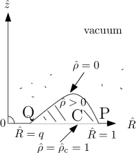
Figure 8: Three points used in the HSCF scheme.

In our numerical studies, the generalized iteration scheme known as Hachisu’s Self-Consistent-Field (HSCF) method (Hachisu 1986) is adopted in order to solve the system of non-linear partial differential equations for equilibrium configurations of magnetized toroids. In this generalized HSCF method, the density, the gravitational potential and the vector potential are discretized on grid points $(r_{i},\theta_{j})$ and non-linear algebraic equations for these discretized physical quantities are iteratively solved (Tomimura & Eriguchi 2005).

We start our computation by assuming initial guesses for the discretized mass density and flux function. Using a trial density and a flux function distribution, the dimensionless gravitational potential $\hat{\phi}_{g}$ and the vector potential $\hat{A}_{\varphi}$ are respectively computed through the integrations, which are equivalent to Eqs. (31) and (32),

$$\hat{\phi}_{g}(\hat{r},\theta) = -\sum_{n=0}^{n_{\max}}\mathrm{P}_{2n}(\cos\theta)\int_{0}^{\infty}d\hat{r}^{\prime}\hat{r}^{\prime 2}f_{2n}(\hat{r},\hat{r}^{\prime})$$ (86)

$$\times \int_{0}^{\pi/2}d\theta^{\prime}\sin\theta^{\prime}\mathrm{P}_{2n}(\cos\theta^{\prime})\hat{\rho}(\hat{r}^{\prime},\theta^{\prime}),$$

$$\hat{A}_{\varphi}(\hat{r},\theta) = 4\pi\sum_{n=1}^{n_{\max}}\frac{\mathrm{P}_{2n-1}^{1}(\cos\theta)}{2n(2n-1)}\int_{0}^{\infty}d\hat{r}^{\prime}\hat{r}^{\prime 2}f_{2n-1}(\hat{r},\hat{r}^{\prime})$$ (87)

$$\times \int_{0}^{\pi/2}d\theta^{\prime}\sin\theta^{\prime}\mathrm{P}_{2n-1}^{1}(\cos\theta^{\prime})\hat{j}_{\varphi}(\hat{r}^{\prime},\theta^{\prime}),$$

$$f_{2n}(\hat{r},\hat{r}^{\prime})=\left\{\begin{array}[]{lr}\hat{r}^{\prime 2n}/\hat{r}^{2n+1},&(\hat{r}\geq\hat{r}^{\prime}),\\ \hat{r}^{2n}/\hat{r}^{\prime 2n+1},&(\hat{r}\leq\hat{r}^{\prime}).\end{array}\right.$$ (88)

Here P${}_{n}(\cos\theta)$ are the Legendre polynomials of degree $n$ and P${}^{1}_{n}(\cos\theta)$ are the associated Legendre functions of order one. In the actual computations, we take $n_{\max}=40$ typically. We use Eq. (45) to obtain the distribution of $\hat{j}_{\varphi}$. After these integrals, we calculate the distribution of the flux function using the relation of Eq. (27). Although there are many constant parameters in our formulation, three constants, the length scale factor $\beta$, the integration constant $\hat{C}$, and the strength of the toroidal current $\hat{\mu}_{0}$ are especial in the sense that they cannot be specified before converged solutions are obtained. These three constants are determined by imposing the following three conditions given at three special grid points and therefore change their values during the iteration procedures. Fig. 8 shows a schematic image of our scheme. At the inner surface (point Q), i.e. at $\hat{r}=q$ and $\theta=\pi/2$, and at the outer surface (point P), i.e. at $\hat{r}=1$ and $\theta=\pi/2$, the density must vanish. At the point where the density takes its maximum value (point C), i.e. at a point of $\hat{r}=\hat{r}_{\mathrm{max}}$ and $\theta=\theta_{\mathrm{max}}$, the dimensionless density must be unity. From Bernoulli’s equation (85) and three conditions are explicitly given by

$$0=-{\hat{\phi}_{g}}|_{P}+\frac{\hat{M}_{c}}{4\pi\hat{r}}\Big{|}_{P}-\frac{1}{2}({\hat{v}_{r}}^{2}+{\hat{v}_{\theta}}^{2}+{\hat{v}_{\varphi}}^{2})|_{P}$$

$$+\frac{\hat{\mu}_{0}}{m+1}(\hat{\Psi}|_{P}+\epsilon)^{m+1}+\hat{r}\sin\theta\hat{v}_{\varphi}\hat{\Omega}_{0}(\hat{\Psi}^{2}+d^{2})^{\alpha}|_{P}+\hat{C}\ ,$$ (89)

$$0=-{\hat{\phi}_{g}}|_{Q}+\frac{\hat{M}_{c}}{4\pi\hat{r}}\Big{|}_{Q}-\frac{1}{2}({\hat{v}_{r}}^{2}+{\hat{v}_{\theta}}^{2}+{\hat{v}_{\varphi}}^{2})|_{Q}$$

$$+\frac{\hat{\mu}_{0}}{m+1}(\hat{\Psi}|_{Q}+\epsilon)^{m+1}+\hat{r}\sin\theta\hat{v}_{\varphi}\hat{\Omega}_{0}(\hat{\Psi}^{2}+d^{2})^{\alpha}|_{Q}+\hat{C}\ ,$$ (90)

$$\beta(1+N)=-{\hat{\phi}_{g}}|_{C}+\frac{\hat{M}_{c}}{4\pi\hat{r}}\Big{|}_{C}-\frac{1}{2}({\hat{v}_{r}}^{2}+{\hat{v}_{\theta}}^{2}+{\hat{v}_{\varphi}}^{2})|_{C}$$

$$+\frac{\hat{\mu}_{0}}{m+1}(\hat{\Psi}|_{C}+\epsilon)^{m+1}+\hat{r}\sin\theta\hat{v}_{\varphi}\hat{\Omega}_{0}(\hat{\Psi}^{2}+d^{2})^{\alpha}|_{C}+\hat{C}\ ,$$ (91)

Solving these equations, we obtain three constants $\beta$, $\hat{C}$ and $\hat{\mu}_{0}$. Using the three constants, gravitational potential and flux function obtained newly, we solve Bernoulli’s equation in terms of the matter density as follows:

$$\hat{\rho}=\Big{(}\dfrac{-{\hat{\phi}_{g}}+\frac{\hat{M}_{c}}{4\pi\hat{r}}-\frac{1}{2}({\hat{v}_{r}}^{2}+{\hat{v}_{\theta}}^{2}+{\hat{v}_{\varphi}}^{2})+\frac{\hat{\mu}_{0}}{m+1}(\hat{\Psi}+\epsilon)^{m+1}+\hat{r}\sin\theta\hat{v}_{\varphi}\hat{\Omega}_{0}(\hat{\Psi}^{2}+d^{2})^{\alpha}+\hat{C}}{\beta(1+N)}\Big{)}^{N}\ .$$ (92)

The newly obtained density and other quantities are used as a new guess for the next potentials in the iteration cycle. We carry out this iteration procedure until the relative changes of all physical quantities between two iteration cycles becomes less than some prescribed small number, e.g., $10^{-4}$.

Appendix E Numerical accuracy check

Figure 9: Values of VC vs. the number of the grid points in the $r$ direction.

In order to check the convergence and the accuracy of the obtained stationary solutions, we use a virial relation,

$$2T+W+3\Pi+\mathfrak{M}=0.$$ (93)

This relation is satisfied for the exact stationary solutions. Numerical solutions, however, have numerical errors. Thus, in general, the right-hand side of Eq. (93) does not vanish although its value should be sufficiently small. In order to quantify numerical errors contained in the numerical solutions obtained, we evaluate a virial relation, defined by

$${\rm VC}=\left|\frac{2\hat{T}+\hat{W}+3\hat{\Pi}+\mathfrak{\hat{M}}}{\hat{W}}\right|.$$ (94)

VC is an estimate of the numerical errors and has been used in many papers (e.g., Hachisu 1986; Tomimura & Eriguchi 2005; Lander & Jones 2009; Otani et al. 2009; Fujisawa et al. 2012). If a value of VC is less than $10^{-4}$ - $10^{-5}$, the solution is considered to be sufficiently accurate. We have checked the convergence of VC by changing the gird number in the $\hat{r}$ direction, $N_{r}$, to test our numerical code in which we have used the spherical coordinates. As for the grid number in the $\theta$ direction, $N_{\theta}$, we fix it as $N_{\theta}=129$ during the test computations. Since we assume equatorial symmetry and the gravitational potential of the central object has a singularity at $\hat{r}=0$, we consider the region defined by $\hat{r}\in[1.0\times 10^{-2}:4.0]$ and $\theta\in[0:\pi/2]$ as our computational space. In order to resolve structures of the toroid properly, we use non-uniformly distributed grid points used in Fujisawa et al. 2012). We compute equilibrium configurations with $q=0.6$, $M_{t}/M_{c}=2.0\times 10^{-2}$, $m=0$, $\hat{\kappa}_{0}=4.5$, $\hat{Q}_{0}=0.0$, $\hat{\Omega}_{0}=0.0$ (no rotation) for several different values of $N_{r}$. Fig. 9 shows values of log VC against values of log $N_{r}$. In this figure, we observe that as the grid number in the $r$-direction is increased, the value of VC becomes smaller as

$${\rm VC}\propto N_{r}^{-2}\,.$$ (95)

This behavior of VC is quite reasonable and proper because we use the numerical scheme with the second-order accuracy formula for numerical derivatives and Simpson’s integration formula. If $N_{r}=513$ ($\log N_{r}\sim 2.710$), the value of VC is $\sim 10^{-5}$ ($\log$ VC $=-4.58$). In the present study, we choose the grid number as $N_{r}=513$ and $N_{\theta}=513$ because this grid number is sufficiently large to obtain numerical solutions with acceptable accuracy as shown before.

References

- Banerjee et al. (1995) Banerjee D., Bhatt J. R., Das A. C., Prasanna A. R., 1995, ApJ, 449, 789
- Baureis et al. (1989) Baureis P., Ebert R., Schmitz F., 1989, A&A, 225, 405
- Bisnovatyi-Kogan & Blinnikov (1972) Bisnovatyi-Kogan G. S., Blinnikov S. I., 1972, Ap&SS, 19, 119
- Bisnovatyi-Kogan & Seidov (1985) Bisnovatyi-Kogan G. S., Seidov Z. F., 1985, Ap&SS, 115, 275
- Chandrasekhar (1956a) Chandrasekhar S., 1956a, ApJ, 124, 232
- Chandrasekhar (1956b) —, 1956b, Proceedings of the National Academy of Science, 42, 1
- Chandrasekhar & Fermi (1953) Chandrasekhar S., Fermi E., 1953, ApJ, 118, 116
- Chandrasekhar & Prendergast (1956) Chandrasekhar S., Prendergast K. H., 1956, Proceedings of the National Academy of Science, 42, 5
- Duez et al. (2006) Duez M. D., Liu Y. T., Shapiro S. L., Shibata M., Stephens B. C., 2006, Phys. Rev. D, 73, 104015
- Eriguchi et al. (1986) Eriguchi Y., Mueller E., Hachisu I., 1986, A&A, 168, 130
- Ferraro (1954) Ferraro V. C. A., 1954, ApJ, 119, 407
- Fujisawa et al. (2012) Fujisawa K., Yoshida S., Eriguchi Y., 2012, MNRAS, 422, 434
- Ghanbari & Abbassi (2004) Ghanbari J., Abbassi S., 2004, MNRAS, 350, 1437
- Gjellestad (1954) Gjellestad G., 1954, ApJ, 119, 14
- Hachisu (1986) Hachisu I., 1986, ApJS, 61, 479
- Hotokezaka et al. (2011) Hotokezaka K., Kyutoku K., Okawa H., Shibata M., Kiuchi K., 2011, Phys. Rev. D, 83, 124008
- Kiuchi et al. (2009) Kiuchi K., Sekiguchi Y., Shibata M., Taniguchi K., 2009, Phys. Rev. D, 80, 064037
- Kyutoku et al. (2011) Kyutoku K., Okawa H., Shibata M., Taniguchi K., 2011, Phys. Rev. D, 84, 064018
- Kyutoku et al. (2010) Kyutoku K., Shibata M., Taniguchi K., 2010, Phys. Rev. D, 82, 044049
- Lander & Jones (2009) Lander S. K., Jones D. I., 2009, MNRAS, 395, 2162
- Li & Shu (1996) Li Z.-Y., Shu F. H., 1996, ApJ, 472, 211
- Lovelace et al. (1986) Lovelace R. V. E., Mehanian C., Mobarry C. M., Sulkanen M. E., 1986, ApJS, 62, 1
- Lüst & Schlüter (1954) Lüst R., Schlüter A., 1954, ZAp, 34, 263
- Narayan et al. (2001) Narayan R., Piran T., Kumar P., 2001, ApJ, 557, 949
- Okada et al. (1989) Okada R., Fukue J., Matsumoto R., 1989, PASJ, 41, 133
- Ostriker (1964) Ostriker J., 1964, ApJ, 140, 1067
- Ostriker & Hartwick (1968) Ostriker J. P., Hartwick F. D. A., 1968, ApJ, 153, 797
- Otani et al. (2009) Otani J., Takahashi R., Eriguchi Y., 2009, MNRAS, 396, 2152
- Prendergast (1956) Prendergast K. H., 1956, ApJ, 123, 498
- Roberts (1955) Roberts P. H., 1955, ApJ, 122, 508
- Sekiguchi & Shibata (2004) Sekiguchi Y., Shibata M., 2004, Phys. Rev. D, 70, 084005
- Sekiguchi & Shibata (2007) —, 2007, Progress of Theoretical Physics, 117, 1029
- Sekiguchi & Shibata (2011) —, 2011, ApJ, 737, 6
- Shibata (2000) Shibata M., 2000, Progress of Theoretical Physics, 104, 325
- Shibata (2003) —, 2003, ApJ, 595, 992
- Shibata & Sekiguchi (2005) Shibata M., Sekiguchi Y., 2005, Phys. Rev. D, 72, 044014
- Shibata et al. (2007) Shibata M., Sekiguchi Y., Takahashi R., 2007, Progress of Theoretical Physics, 118, 257
- Shibata & Shapiro (2002) Shibata M., Shapiro S. L., 2002, ApJ, 572, L39
- Shibata & Taniguchi (2008) Shibata M., Taniguchi K., 2008, Phys. Rev. D, 77, 084015
- Shibata et al. (2003) Shibata M., Taniguchi K., Uryū K., 2003, Phys. Rev. D, 68, 084020
- Shibata et al. (2005) —, 2005, Phys. Rev. D, 71, 084021
- Shibata & Uryū (2006) Shibata M., Uryū K., 2006, Phys. Rev. D, 74, 121503
- Shibata & Uryū (2000) Shibata M., Uryū K. ō., 2000, Phys. Rev. D, 61, 064001
- Shibata & Uryu (2007) Shibata M., Uryu K., 2007, Classical and Quantum Gravity, 24, 125
- Sykes (1957) Sykes J., 1957, ApJ, 125, 615
- Tomimura & Eriguchi (2005) Tomimura Y., Eriguchi Y., 2005, MNRAS, 359, 1117
- Woltjer (1959a) Woltjer L., 1959a, ApJ, 130, 400
- Woltjer (1959b) —, 1959b, ApJ, 130, 405
- Woltjer (1960) —, 1960, ApJ, 131, 227
- Wong (1974) Wong C.-Y., 1974, ApJ, 190, 675
- Yoshida & Eriguchi (2006) Yoshida S., Eriguchi Y., 2006, ApJS, 164, 156
- Yoshida et al. (2006) Yoshida S., Yoshida S., Eriguchi Y., 2006, ApJ, 651, 462