Coexistence of oppositely flowing multi-$\varphi$-currents: Key to large toroidal magnetic fields within stars

Abstract

We will show the importance of coexistence of oppositely flowing $\varphi$-currents for magnetized stars to sustain strong toroidal magnetic fields within the stars by analyzing stationary states of magnetized stars with surface currents which flow in the opposite direction with respect to the bulk currents within the stars. We have imposed boundary conditions for currents and toroidal magnetic fields to vanish outside the stars. It is important to note that these boundary conditions set an upper limit for the total current within the stars. This upper limit for the total current results in the presence of an upper limit for the magnitude of the energy for the toroidal magnetic fields of the stars. If the stars could have the toroidal surface currents which flow in the opposite directions to the internal toroidal currents, the positively flowing internal toroidal currents can become stronger than the upper limit value of the current for configurations without surface toroidal currents. Thus the energies for the toroidal magnetic fields can become much larger than those for the magnetized stars without surface toroidal currents. We have also analyzed the same phenomena appearing in spherical incompressible stars for dipole-like magnetic fields with or without surface toroidal currents by employing the zero-flux-boundary method. We have applied those configurations with surface toroidal currents to magnetars and discussed their flares through which magnetic helicities could arise outside the stellar surfaces.

1 Introduction

The origin of the magnetic fields inside the star is not still understood well. According to the recent progresses of the theoretical researches, there are two possibilities for the mechanism to generate and sustain magnetic fields, i.e. 1) the dynamo theory and 2) the fossil field theory (see the review by Moss 1994). Stars which have convective regions regenerate and sustain the magnetic fields by the dynamo mechanism. On the other hand, A, B, O stars have a convective core where dynamo action develops (e.g. Brun et al. 2005 ). However, the timescale for the dynamo-generated field in this core to reach the surface is too long (Charbonneau & MacGregor 2001). Therefore the magnetic field observed at the stellar surface is supposed to be fossil field. Recent observations show the observed magnetic fields’ properties confirm this hypothesis (see Wade et al. 2011). Consequently, it has long been considered that magnetic fields of such stars would come from fossil magnetic fields. According to the fossil field theory, the magnetic fields of such stars would be originated from magnetized interstellar media. If the magnetic fluxes would be conserved during star formation processes, the magnetic fields could be concentrated to smaller regions of the stars by the gravitational contraction and result in strong magnetic fields inside the stars. Since the electric conductivities of the stars are very large, those magnetic fields do not diffuse during their formation stages. As for neutron stars, the origin of their strong magnetic fields is much more uncertain. If the fossil field theory could be applied, the strong magnetic fields could be reached by the same mechanism as those mentioned above for stars without external convective regions. On the other hand, if we could adopt the dynamo theory, the strong magnetic fields would be formed by the dynamo due to the rapid differential rotations in the convective regions of the proto-neutron stars (Duncan & Thompson 1992). The differential rotations could wind up the initial poloidal magnetic fields to produce strong toroidal magnetic fields before the crusts would crystallize. In either case, the magnetic fields of neutron stars would be present even at birth and survive in much longer timescales than the Alfvén timescale ($=\sqrt{4\pi\rho}r_{s}/B\sim 100$ s for typical neutron stars with magnetic fields of order of $B=10^{12}$G). Here $r_{s}$ is the radius of the stellar surface which is, for axisymmetric configurations, a function of $\theta$ of the polar coordinates $(r,\theta,\varphi)$, i.e. $r_{s}(\theta)$. In order to sustain these kinds of fossil magnetic fields for a long time, these magnetic fields must be stationary and stable. Thus, in order to understand the magnetic fields originated from the fossil fields, it would be useful and important to get stationary and stable configurations of magnetized stars.

As for stability, analytic studies have shown that any configurations with either purely poloidal or purely toroidal magnetic fields are unstable (Tayler 1973; Markey & Tayler 1973). Stable magnetized stars should have both the poloidal and the toroidal magnetic fields. Moreover, the magnitudes of the toroidal fields must be comparable with those of the poloidal fields (Tayler 1980). This argument has been shown to be the case from the recent simulations. Braithwaite & Spruit (2004) have shown that an initial random magnetic field in stably stratified stellar layers relaxes on the stable twisted-torus magnetic field configuration after several Alfvén timescale. Similar twisted-torus magnetic field configurations have been also obtained in many previous works by numerically exact computations of the axisymmetric stationary states of magnetized stars (Tomimura & Eriguchi 2005; Yoshida & Eriguchi 2006; Lander & Jones 2009; Lander et al. 2011; Fujisawa et al. 2012), structure separated Grad-Shafranov (GS) solving method (Ciolfi et al. 2009; Glampedakis et al. 2012) or zero-flux-boundary method (Prendergast 1956; Ioka & Sasaki 2004; Duez & Mathis 2010; Yoshida et al. 2012). The stabilities of these fields, however, have not been clarified yet because it is difficult to analyze their stability by linear stability analyses or other means based on the stationary configurations. On the other hand, Braithwaite (2009) and Duez et al. (2010) have shown that the stability criteria of the magnetized stars could be expressed as below:

$$a\frac{{\cal M}}{|W|}<\frac{{\cal M}_{p}}{\cal M}\leq 0.8,$$ (1)

where ${\cal M}/{|W|}$ is the ratio of the magnetic energy to the gravitational energy (see Appendix A.1). ${\cal M}_{p}/{\cal M}$ is the ratio of the poloidal magnetic energy to the total magnetic energy and $a$ is a certain dimensionless factor of order 10 for main-sequence stars and of order $10^{3}$ for neutron stars. The value of ${\cal M}/{|W|}$ is about $10^{-6}$ even for magnetars and is expected to be ${\cal M}/{|W|}<10^{-6}$ for other real stars. Thus the left hand side of this inequality could be less than about $10^{-3}$ even if the value of $a$ might be $\sim 1000$. Therefore, this criterion means the configurations with the twisted torus magnetic fields are stable even if the toroidal magnetic fields are much stronger than the poloidal magnetic fields. In contrast, the right hand side of this inequality means that the strong poloidal magnetic field configurations are unstable (we define that the poloidal fields are strong when ${\cal M}_{p}/{\cal M}>0.8$ in this paper). As shown in dynamical simulations mentioned above, configurations with the strong poloidal magnetic fields are likely to become unstable within several Alfvén timescales. This criteria would not be applied to all situations because we might be able to consider various kinds of magnetic field configurations as the initial states and different choices of the initial conditions might influence on the evolutions of the magnetic fields. However, it seems to be the case that there is a tendency to become more unstable even for the twisted-torus magnetic field configurations with larger poloidal magnetic field energies. Therefore, it would be a natural consequence to consider that there would be stable magnetized stars with strong toroidal magnetic fields which satisfy the condition ${\cal M}_{p}/{\cal M}<0.8$, i.e. ${\cal M}_{t}/{\cal M}>0.2$ where ${\cal M}_{t}$ is the energy of the toroidal field.

On the other hand, the majority of investigations in which stationary states of the magnetized stars have been treated (e.g. Yoshida & Eriguchi 2006; Yoshida et al. 2006; Lander & Jones 2009; Ciolfi et al. 2009; Lander et al. 2011; Fujisawa et al. 2012) failed to obtain configurations with strong toroidal magnetic fields. In these studies, stationary states of magnetized stars have been pursued either by numerically exact methods (e.g. Tomimura & Eriguchi 2005) or structure separated GS solving methods (e.g. Ciolfi et al. 2009). However, they have only found that it was very difficult to obtain stationary states of magnetized stars with very strong toroidal magnetic fields. In some of their solutions the toroidal magnetic fields have been almost as strong as the poloidal magnetic fields only in the particular local regions inside the stars, but the total energies of the toroidal magnetic fields as a whole are much smaller than those of the total poloidal magnetic fields. In other words, the ratios of ${\cal M}_{p}/{\cal M}$ in their solutions are much bigger than 0.8.

By contrast, some studies of magnetized stationary configurations by structure separated GS solving method (Glampedakis et al. 2012) by zero-flux-boundary method (Duez & Mathis 2010; Yoshida et al. 2012) have succeeded in obtaining the magnetized equilibria with strong toroidal magnetic fields by choosing very special boundary conditions for the poloidal magnetic fields. The boundary condition adopted by Tomimura & Eriguchi (2005) and Ciolfi et al. (2009) in which they failed to obtain configurations with strong toroidal magnetic fields is that the poloidal magnetic field lines should continue smoothly through the stellar surfaces into the vacuum region which is considered to be outside of the stars. On the other hand, the boundary condition employed by Glampedakis et al. (2012) is different. The poloidal magnetic field lines need not continue smoothly at the stellar surfaces, because in some of their models it has been allowed for the surface currents to exist. By specifying such a boundary condition, they have succeeded in finding that magnetized configurations whose total energies of the toroidal magnetic fields become much stronger as the surface currents are increased.

Duez & Mathis (2010) and Yoshida et al. (2012) also obtained the stationary configurations with strong toroidal magnetic fields, but the boundary condition which they adopted is of different kind from those mentioned above. Their assumptions are essentially the same as those in the previous works (Prendergast 1956; Woltjer 1959a, b, 1960; Ioka & Sasaki 2004). They imposed the boundary condition that the magnetic flux on the stellar surfaces should vanish, so all of poloidal field lines are closed and confined inside the stars and no poloidal magnetic fields penetrate to the vacuum region outside of stars. In their solutions, the region where the toroidal magnetic fields exist inside the star is much larger than that of any other models. However, they did not explain the reason why the magnetized stars can sustain such configurations with large toroidal magnetic energies under their special boundary condition.

In this paper we will deal with magnetized configurations with large amount of the magnetic energies in the toroidal fields and present the reason why the magnetized stars can sustain strong toroidal magnetic fields within the stars. As will be shown, we have found that the total currents of the magnetized stars are important keys to understand this problem systematically and the values of the total currents seem to be deeply related to the boundary condition of the magnetic fields.

It should be noted that for the stationary configurations the magnetic fields are governed by the Grad-Shafranov equation which is of the elliptic type partial differential equation for the magnetic flux function. Therefore, the solutions of the GS equation are necessarily strongly depending on the boundary condition(s).

In this paper, we use both the numerically exact non-force-free method (Tomimura & Eriguchi 2005) and the method in which boundary conditions are applied at finite locations from the stellar centre (e.g., Prendergast 1956; Ioka & Sasaki 2004; Duez & Mathis 2010). We will show configurations with negative surface currents or with the regions where the current become negative can sustain the strong toroidal magnetic fields inside the star. Here the term ’negative’ means that the currents flow in the opposite direction to the flow direction of the bulk of the interior currents.

2 Formulation

Our formulation of the problem  and the numerical methods are essentially the same as that of Tomimura & Eriguchi (2005), i.e. the numerically exact method, and that of Duez & Mathis (2010), i.e. the zero-flux-boundary method.

2.1 Grad-Shafranov equation

We calculate self-gravitating, axisymmetric, stationary magnetized stars in order to obtain magnetized equilibria with strong toroidal fields in the Newtonian gravity. We assume that the system is in a stationary and axisymmetry state. For rotating stars, the rotational axis and the magnetic axis coincide and the rotation is assumed to be rigid. The star has no meridional flows. The conductivity of the stellar matter is infinite, i.e. the ideal MHD approximation is employed. There is no magnetosphere around the star. In other words, no electric current exists in the vacuum region. Therefore, the toroidal magnetic field is confined within the star and the only poloidal component can penetrate the surface and extend to the outside of the star. We use the polytropic equation of state as below:

$$p=K\rho^{1+1/N}.$$ (2)

Here $p$, $\rho$, $K$ and $N$ are the pressure, the mass density, the polytropic constant and the polytropic index, respectively. We fix $N=1$ for simplicity when we compute stationary configurations by using the numerically exact method. This choice of $N$ is the same as that adopted in the previous works (e.g. Lander & Jones 2009).

We introduce the magnetic flux function $\Psi$ in order to obtain magnetized equilibria efficiently. The magnetic flux function is defined as below:

$$B_{r}\equiv\frac{1}{r^{2}\sin\theta}\dfrac{\partial\Psi}{\partial\theta},\hskip 10.0ptB_{\theta}\equiv-\frac{1}{r\sin\theta}\dfrac{\partial\Psi}{\partial r}\ ,$$ (3)

where $B_{r}$ and $B_{\theta}$ are the components of the magnetic field in the $r$-direction and the $\theta$-direction, respectively. Using the flux function $\Psi$, we derive the Grad-Shafranov equation from Maxwell equations as follows:

$$\Delta^{*}\Psi\equiv\dfrac{\partial^{2}\Psi}{\partial r^{2}}+\frac{\sin\theta}{r^{2}}\dfrac{\partial}{\partial\theta}\left(\frac{1}{\sin\theta}\dfrac{\partial\Psi}{\partial\theta}\right)=-4\pi r\sin\theta\frac{j_{\varphi}}{c},$$ (4)

where $j_{\varphi}$ and $c$ are the $\varphi$-component of the current and the speed of light, respectively.

The magnetic flux function $\Psi$ can be expressed as:

$$\Psi=r\sin\theta A_{\varphi}\ ,$$ (5)

where $A_{\varphi}$ is the $\varphi$-component of the vector potential which satisfies $\nabla\times\mbox{\boldmath$A$}\equiv\mbox{\boldmath$B$}$. The form of Grad-Shafranov equation can be rewritten as:

$$\Delta(A_{\varphi}\sin\varphi)=-\frac{4\pi}{c}j_{\varphi}\sin\varphi,$$ (6)

where, $\Delta$ denotes the ordinary Laplacian operator. This equation seems strange because the system treated in this paper is axisymmetric and $\varphi$-dependency would not appear. The reason why we introduce the term $\sin\varphi$ is that by introducing the $\sin\varphi$ term we can get an equation which contains the three dimensional Laplacian operator as shown above. The tree dimensional Laplacian operator which emerges by this seemingly ’strange’ device allows us to transform the equation into an integral form as shown below. By taking the boundary condition for the vector potential into account and using Green’s function which satisfies the boundary condition, we derive the integral form of the GS equation as follows:

$$A_{\varphi}(\mbox{\boldmath$r$})\sin\varphi=\frac{1}{c}\int\frac{j_{\varphi}(\mbox{\boldmath$r$}^{\prime})}{|\mbox{\boldmath$r$}-\mbox{\boldmath$r$}^{\prime}|}\sin\varphi^{\prime}\,d^{3}\mbox{\boldmath$r$}^{\prime}+A_{\varphi,h}(r,\theta)\sin\varphi,$$ (7)

where $A_{\varphi,h}$ is a homogeneous general solution to Eq.(6) as follows:

$$A_{\varphi,h}(r,\theta)=\sum_{n=0}^{\infty}\Big{[}a_{n}\frac{r_{0}^{n+2}}{r^{n+1}}+b_{n}\frac{r^{n}}{r_{0}^{n-1}}\Big{]}P_{n}^{1}(\cos\theta).$$ (8)

Here, $r_{0}$ is a certain constant which is the stellar radius for spherical configurations, and $a_{n}$ and $b_{n}$ are constant coefficients which are obtained by applying the boundary condition. We will be able to obtain the stationary distributions of the magnetic vector potentials by solving this equation. Since these equations are of elliptic type partial differential equations whose source term is $j_{\varphi}$, the boundary conditions are very important and have significant influences on the global structures of the vector potentials or the magnetic flux functions. We will deal with this problem about the boundary condition in Sec. 3.

2.2 Toroidal magnetic fields

Once we have obtained the flux function by solving the GS equation, it is easy to calculate the poloidal magnetic fields directly. On the other hand, we can obtain the toroidal component of the magnetic field by using the conserved quantity along the flux function which can be expressed by an arbitrary function of $\Psi$. This arbitrary function appears because of the assumption of the axisymmetry. This function is called $\kappa(\Psi)$ in Tomimura & Eriguchi (2005), $F$ in Duez & Mathis (2010) and $T$ in Glampedakis et al. (2012). In this paper we name it $\kappa(\Psi)$ after Tomimura & Eriguchi (2005). The toroidal component of the magnetic field is obtained from the following relation

$$B_{\varphi}=\frac{\kappa(\Psi)}{r\sin\theta}.$$ (9)

This arbitrary function also appears in the expression of the current density as follows:

$$\frac{\mbox{\boldmath$j$}}{c}=\frac{1}{4\pi}\dfrac{d\kappa(\Psi)}{d\Psi}\mbox{\boldmath$B$}+\rho r\sin\theta\mu(\Psi)\mbox{\boldmath$e$}_{\varphi}\ ,$$ (10)

where, $\mu(\Psi)$ is another arbitrary function of $\Psi$. The arbitrary function $\mu(\Psi)$ is the same as $G$ in Duez & Mathis (2010) and $F$ in Glampedakis et al. (2012). Then, we express the $\varphi$ component of the current density as below:

$$\frac{j_{\varphi}}{c}=\frac{1}{4\pi}\dfrac{d\kappa(\Psi)}{d\Psi}\frac{\kappa(\Psi)}{r\sin\theta}+\rho r\sin\theta\mu(\Psi)\ .$$ (11)

The first term of Eq.(11) is the force-free current density part and the second term is the non-force-free current part because of $\nabla\times\mbox{\boldmath$B$}=4\pi\mbox{\boldmath$j$}/c$. If $\mu=0$ in a certain region, the magnetic field there is force-free, because $\mbox{\boldmath$j$}\propto\alpha\mbox{\boldmath$B$}$ in that region. We will call the first term as the $\kappa$ term, and the second term as the $\mu$ term of the current density in this paper. In a naive treatment, it seems to be enough to make the contribution from the $\kappa$ term larger in order to make the toroidal magnetic fields larger. However, it has been very difficult to make the influence from the $\kappa$ term strong. The reason for that is as follows. The distribution of $\Psi$ is obtained by solving the GS equation, but the source term of the GS equation contains the $\kappa$ term which is an arbitrary function of $\Psi$ and is confined to a restricted region in the interior of the star because we impose the magnetic flux function to be smoothly connected on the stellar surface. Therefore, if we change the functional form and values of parameters which appear in the functional form of $\kappa$ as well as the the region where $\kappa$ does not vanish, the distribution of the flux function also changes according to the changes of $\kappa$. We will discuss this difficulty in Sec.4.2.

3 Surface currents

In this section, we deal with the relation between the surface current and the magnetic field, which is deeply influenced by the boundary conditions. The surface current can be defined either by the discontinuity of the derivative of the magnetic flux function, or by the homogeneous term in the integral representation for the vector potential. The both definitions for the surface current give exactly the same values as we will see later.

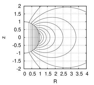
Figure 1: Poloidal magnetic field lines with a purely dipole (n=1) surface current (left) and a purely quadrupole $(n=2)$ surface current (right).

3.1 Relation between the surface current and the discontinuity of the magnetic field

At first, we will show a relation between the surface current and the discontinuity of the magnetic field as follows. If the Ampére’s equation is applied to an area $S$ bounded by a boundary $\partial S$, we can write it by an integral form as follows:

$$\oint_{\partial S}\mbox{\boldmath$B$}\cdot d\mbox{\boldmath$\ell$}=\frac{4\pi}{c}\int_{S}\mbox{\boldmath$j$}\cdot d\mbox{\boldmath$S$},$$ (12)

where $d\mbox{\boldmath$\ell$}$ and $d\mbox{\boldmath$S$}$ are a line element and a surface element, respectively. We apply this equation to an infinitely small area in the meridional plane of the star bounded by four lines as follows:

$$r = r_{s}(\theta_{1})-\frac{\Delta r}{2}\ ,$$ (13)

$$r = r_{s}(\theta_{1})+\frac{\Delta r}{2}\ ,$$ (14)

$$\theta = \theta_{1}\ ,$$ (15)

$$\theta = \theta_{1}+\Delta\theta\ ,$$ (16)

where $\theta_{1}$, $\Delta r$ and $\Delta\theta$ are a constant, infinitesimal widths in the $r$-direction and in the $\theta$-directions, respectively. For this infinitesimal area, we obtain

$$\Big{[}B_{r}^{ex}(r_{s},\theta)-B_{r}^{in}(r_{s},\theta)\Big{]}\Delta r+\Big{[}B_{\theta}^{ex}(r_{s},\theta)-B_{\theta}^{in}(r_{s},\theta)\Big{]}r_{s}\Delta\theta$$ (17)

$$= \frac{4\pi}{c}\int_{r_{s}-\Delta r/2}^{r_{s}+\Delta r/2}j_{\varphi}(r,\theta)r\,dr\Delta\theta,$$

where $B^{ex}$ and $B^{in}$ are the exterior and interior values of the magnetic fields. Here, if the current density is a surface current on the stellar surface $(r=r_{s}(\theta))$ defined by $j_{\varphi}(r,\theta)=j_{sur}(\theta)\delta(r-r_{s}(\theta))$, we can integrate the equation as below

$$\int_{r_{s}-\Delta r/2}^{r_{s}+\Delta r/2}j_{\varphi}(r,\theta)r\,dr$$ (18)

$$= \int_{r_{s}-\Delta r/2}^{r_{s}+\Delta r/2}j_{sur}(\theta)\delta(r-r_{s})r\,dr=r_{s}j_{sur}(\theta).$$

Since the $r$ dependence of the magnetic fields are continuous on the stellar surface ($r=r_{s}(\theta)$), we obtain a relation as follows:

$$B_{\theta}^{ex}(r_{s},\theta)-B_{\theta}^{in}(r_{s},\theta)=\frac{4\pi}{c}j_{sur}(\theta).$$ (19)

The surface current is expressed by the discontinuity of the $\theta$-component of the magnetic field. For more general situations, we can obtain the following equation for the surface current using the parallel component $B_{||}$ to the stellar surface,

$$B_{||}^{ex}(r_{s},\theta)-B_{||}^{in}(r_{s},\theta)=\frac{4\pi}{c}j_{sur}(\theta).$$ (20)

If the surface current exits, the parallel component of the magnetic field must be discontinuous. We emphasize that the value of the discontinuity of the magnetic field between just inside and just outside of the stellar surface equals the surface current density.

Glampedakis et al. (2012) expressed the surface current density in a different way as follows. They defined the surface current by imposing the discontinuity of poloidal magnetic fields at the stellar surface (see Eq.67 in Glampedakis et al. 2012). Their discontinuous boundary condition is just an assumption without a firm foundation as follows:

$$b^{in}_{\theta}=\xi b^{ex}_{\theta}\Leftrightarrow b_{\theta}^{ex}-b_{\theta}^{in}=(1-\xi)b_{\theta}^{ex}=j_{sur}.$$ (21)

Here $b$ and $\xi$ indicate the magnetic field and a discontinuity parameter, respectively, in their paper. Since their model is a purely dipole configuration, the exterior solution of $b_{\theta}$ is $b_{\theta}^{ex}(x)=\frac{1}{2x}d\hat{\alpha}/dx\sin\theta$ (Eq.61 in Glampedakis et al. 2012). Here $\alpha$ and $x$ indicate the $r$-component of the flux function and the dimensionless radius normalized by the stellar radius. Then we can calculate the distribution of their surface current density as follows,

$$j_{sur}=\left[(1-\xi)\frac{1}{2x}\dfrac{d\alpha}{dx}\sin\theta\right]_{(x=1)}=-j_{0}\sin\theta,$$ (22)

where

$$j_{0}=\left[(\xi-1)\dfrac{1}{2x}\dfrac{\partial\hat{\alpha}}{\partial x}\right]_{(x=1)}.$$

Since they calculated only models with $\xi>1$ in their paper, the surface current density of their models flows in the opposite direction to the interior bulk toroidal current density inside the star. In other words their surface current is negatively flowing with respect to the bulk interior currents. According to Glampedakis et al. (2012), if the value for the discontinuity for the poloidal magnetic field is increased, the energy of the toroidal magnetic fields becomes larger (see Fig. 5 in Glampedakis et al. 2012). Therefore we conclude that the negative surface current sustain strong toroidal magnetic fields comparing with those in Tomimura & Eriguchi models without surface currents.

3.2 Surface currents in the integral representation

Using the integral representation for the vector potential, we can see the surface current from a different point of view. We assume that a magnetized star has no currents in the stellar interior except for the surface current. It implies that the source term for the GS equation consists only of the surface current. We can obtain the magnetic field by calculating Eq. (7),

$$A_{\varphi}\sin\varphi=\frac{1}{c}\int\frac{j_{sur}(r^{\prime},\theta^{\prime})}{|\mbox{\boldmath$r$}-\mbox{\boldmath$r$}^{\prime}|}\sin\varphi^{\prime}\,d^{3}\mbox{\boldmath$r$}^{\prime}.$$ (23)

Since the surface current exists on the stellar surface $r=r_{s}$, we can describe the surface current density using the Dirac’s delta function:

$$\frac{j_{sur}(r^{\prime},\theta^{\prime})}{c}=\delta(r^{\prime}-r_{s})j_{sur}(\theta^{\prime})\ ,$$ (24)

where $j_{sur}(\theta)$ is the surface current which flows along the surface. We can expand and integrate Eq.(23) using the Legendre functions and the axisymmetry of the system. We obtain the solutions for $A_{\varphi}$ as follows:

$$A_{\varphi}(r,\theta) = \sum_{n=1}^{\infty}\dfrac{2\pi}{n(n+1)}P_{n}^{1}(\cos\theta)f_{n}(r,r_{s})r_{s}^{2}$$ (25)

$$\int_{0}^{\pi}\sin\theta^{\prime}P_{n}^{1}(\cos\theta^{\prime})j_{sur}(\theta^{\prime})\,d\theta^{\prime},$$

where $f_{n}$ is a function defined by

$$f_{n}(r,r_{s})=\left\{\begin{array}[]{lr}r_{s}^{n}/r^{n+1},&(r\geq r_{s})\\ r^{n}/r_{s}^{n+1}.&(r\leq r_{s})\end{array}\right.$$ (28)

Now we calculate the vector potential and the magnetic field by giving a $\theta$-distribution for the surface current density. We assume the $\theta$-distribution of the surface current can be expressed by the expansion using Legendre functions,

$$j_{sur}(\theta)=\sum_{n=1}^{\infty}\frac{2n+1}{4\pi}\alpha_{n}P_{n}^{1}(\cos\theta),$$ (29)

where $\alpha_{n}$’s are dimensionless coefficients related to the $n$th associate Legendre function $P_{n}^{1}(\cos\theta)$. Then using the orthogonality among the Legendre functions,

$$\int_{0}^{\pi}\sin\theta^{\prime}P_{n}^{1}(\cos\theta^{\prime})P_{n}^{1}(\cos\theta^{\prime})\,d\theta^{\prime}=2\frac{(n+1)n}{2n+1},$$ (30)

we can obtain an analytically expressed solutions as follows:

$$A_{\varphi}(r,\theta)=\sum_{n=1}^{\infty}\alpha_{n}r_{s}^{2}f_{n}(r,r_{s})P_{n}^{1}(\cos\theta),$$ (31)

and

$$\Psi(r,\theta)=\sum_{n=1}^{\infty}\alpha_{n}rr_{s}^{2}f_{n}(r,r_{s})P_{n}^{1}(\cos\theta)\sin\theta.$$ (32)

If we set $\alpha_{n}=a_{n}+b_{n}$, the right hand side of Eq. (31) is exactly the same as homogeneous general solutions of Eq. (8). Therefore, adding the homogeneous term to the inhomogeneous solution of the GS equation corresponds exactly to adding the surface current at the boundary surface.

Fig. 1 shows the poloidal magnetic field lines for configurations with the purely dipole ($n=1$) surface current (left panel) and with the purely quadrupole ($n=2$) surface current (right panel). It should be noted that each model has no interior currents except for the surface currents as we have described in this section.

4 Numerically exact configurations for open magnetic fields with surface currents

We will show numerically exact structures of magnetized stars with open field lines and with/without surface currents in this section. At first, we will display configurations which have no surface currents. Although they are the same as those obtained in Yoshida & Eriguchi (2006) and Lander & Jones (2009), we will check these models from a different point of view, i.e. in the context of the influence of the surface currents. Next, magnetized stars which have surface currents will be treated and discussed.

4.1 Setting of the problem

As discussed before, we have solved the integral equation derived from the GS equation by considering the presence of the surface currents as follows:

$$A_{\varphi}(\mbox{\boldmath$r$})\sin\varphi=\frac{1}{c}\int\frac{j_{\varphi}(\mbox{\boldmath$r$}^{\prime})+j_{sur}(\mbox{\boldmath$r$}^{\prime})}{|\mbox{\boldmath$r$}-\mbox{\boldmath$r$}^{\prime}|}\sin\varphi^{\prime}\,d^{3}\mbox{\boldmath$r$}^{\prime}\ ,$$ (33)

where $j_{sur}$ is the surface current density of the magnetized star. We choose the following two different distributions for the surface currents:

$$\frac{j_{sur}(r,\theta)}{c}=-j_{0}\sin\theta\delta(r-r_{s}(\theta)),\ (\mbox{dipole distribution})\ ,$$ (34)

and

$$\frac{j_{sur}(r,\theta)}{c}=-j_{0}\sin\theta\cos\theta\delta(r-r_{s}(\theta)).\ (\mbox{quadrupole distribution})\$$ (35)

As for the arbitrary functions appearing in our formulation, we choose the following forms:

$$\mu(\Psi) = \mu_{0}\ ,$$ (36)

$$\int\mu(\Psi)\,d\Psi = \mu_{0}\Psi\ ,$$ (37)

$$\kappa(\Psi)=\left\{\begin{array}[]{ll}0,&\mathrm{for}\ \Psi\leq\Psi_{V\max}\ ,\\ \dfrac{\kappa_{0}}{k+1}(\Psi-\Psi_{V\max})^{k+1},&\mathrm{for}\ \Psi>\Psi_{V\max}\ ,\end{array}\right.$$ (40)

and

$$\kappa^{\prime}(\Psi)=\left\{\begin{array}[]{ll}0,&\mathrm{for}\ \Psi\leq\Psi_{V\max}\ ,\\ \kappa_{0}(\Psi-\Psi_{V\max})^{k},&\mathrm{for}\ \Psi>\Psi_{V\max}\ ,\\ \end{array}\right.$$ (43)

Here, $\mu_{0}$, $k$ and $\kappa_{0}$ are constant parameters and $\Psi_{V\max}$ means the maximum value of $\Psi$ in the vacuum region. In this paper, we fix $k=0.1$. These functional forms and the value of $k$ are the same as those chosen in other papers (Yoshida & Eriguchi 2006; Lander & Jones 2009). In this section, we set the polytropic index $N=1$ (e.g. Lander & Jones 2009), and $q=0.9$ where $q$ is the ratio of the polar radius to the equatorial radius defined by (see Fujisawa et al. 2012)

$$q\equiv\frac{r_{s}(\theta=0)}{r_{s}(\theta=\pi/2)}.$$ (44)

Concerning the angular velocity $\Omega$, we choose values of $\hat{\Omega}=\mbox{constant}\equiv\hat{\Omega}_{0}=1.0$E-2 for rigidly rotating configurations and $\hat{\Omega}_{0}=0.0$ for non-rotating models. Here quantities with $\hat{}$ represent the corresponding ones transformed into dimensionless forms as shown in Appendix A.2 (see also Fujisawa et al. 2012).

Although the equations of state influence the strengths of the toroidal magnetic fields (see Kiuchi & Kotake 2008), we have treated only $N=1$ polytropes because the main concern in this paper is how the surface current density affects the distributions of the magnetic fields, in particular to the toroidal magnetic fields. In order to examine the accuracies of solutions, we have used the virial relation as shown in Appendix A.3.

4.2 Configurations without surface currents

Figure 2: The ratio of the poloidal magnetic energy to the total magnetic energy against the parameter $\hat{\kappa}_{0}$. The solid line denotes a rigidly rotating sequence with $\hat{\Omega}_{0}=1.0$E-2.0 and the dashed line denotes a non-rotating sequence, i.e. a sequence with $\hat{\Omega}_{0}=0.0$. Minimum values seem to be attained at $\hat{\kappa}_{0}\sim 40$ (for the non-rotating sequence) and $\hat{\kappa}_{0}\sim 45$ (for the rigidly rotating sequence).

Figure 3: Left panels: Distributions of the components of the magnetic field [$\hat{B}_{r}(\theta=0),\hat{B}_{\theta}(\theta=\pi/2),\hat{B}_{\varphi}(\theta=\pi/2)$] are shown. Right panels : Distributions of the two source terms on the equator, which appear in the current density formula, are shown. Chosen values of $\hat{\kappa}$ are $\hat{\kappa}_{0}=10$ (top) and $\hat{\kappa}_{0}=65$ (bottom).

Since the value of $\hat{\kappa}_{0}$ affects the local behavior of the toroidal magnetic field distributions, in particular on its maximum value (see Lander & Jones 2009), we have solved the magnetized configurations by changing the value of $\hat{\kappa}_{0}$ for two values of $\hat{\Omega}_{0}$.

Obtained results are plotted in Fig.2 which shows the ratio of ${\cal M}_{p}/{\cal M}$ against $\hat{\kappa}_{0}$. As seen from this figure, there is a minimum value of the ratio. It implies that the toroidal magnetic field energy increases to its maximum value at $\hat{\kappa_{0}}\sim 40$ for non-rotating configurations and at $\hat{\kappa}_{0}\sim 45$ for rigidly rotating models. Since the term related to the rotation does not appear in the current density formula (see Eq.10), the rotation affects the toroidal magnetic field distributions only slightly. Therefore, we will display and discuss only configurations with rotation in the following part of this section.

In many investigations which have been done by applying numerically exact methods or by structure separated GS solving method zero-flux-boundary methods, almost similar results as ours shown in Fig. 2 have been obtained (see Table 2 in Lander & Jones 2009, Fig. 12 in Ciolfi et al. 2009, Fig. 4 in Glampedakis et al. 2012). Therefore, this behavior of the toroidal magnetic field against the value of $\hat{\kappa_{0}}$ is likely to be a general feature of stationary magnetized stars which have open magnetic fields.

In order to consider the reason of the presence of these minimum values, in Fig.3 shown are the distributions of the magnetic field components (left panels) and those of the two components of the current density formula (right panels). Different curves in the left panels mean $\hat{B}_{r}(\theta=0)$ (dotted line), $\hat{B}_{\theta}(\theta=\pi/2)$(dashed line) and $\hat{B}_{\varphi}(\theta=\pi/2)$(solid line) distributions for the region $\hat{r}[0:1.0]$. In the right panels, the solid line denotes the force-free $\kappa$ term and the dashed line denotes the non-force-free $\mu$ term in the current density formula.

As seen from these panels, by increasing the value of $\hat{\kappa}_{0}$, which corresponds to increasing the maximum strength of the toroidal magnetic field, from top panels to bottom panels, we can find that the width of the toroidal magnetic field region becomes narrower. The values of the toroidal magnetic field energy seem to depend on the distributions of the toroidal magnetic fields and of the current densities, in particular, on the maximum value and the width of the toroidal magnetic field distribution. Although the maximum value of the $\kappa$ term of the current density increases with $\hat{\kappa}_{0}$, its width becomes narrower as $\hat{\kappa}_{0}$ is increasing. It implies that the slope of the distribution of the $\kappa$ term becomes steeper for the large value of the current density. This tendency is also seen in the distribution of $B_{\varphi}$. By contrast with this, the distributions of the $\mu$ term are almost the same because we fix $q$ and $\hat{\Omega}_{0}$ which are related to the characteristic nature of the non-force-free magnetic fields.

From Eq. (10) and our numerical results, we can find that in order to sustain strong toroidal magnetic fields (appearing in the right hand side of the equation), the strong toroidal current density (appearing in the left hand side of the equation) is required. It should be noted that the strength of the toroidal magnetic field seems to be related deeply to the strength of the total current density. This can be seen from the following argument. We introduce several definitions about integrated currents as follows:

$$\hat{J}_{tot}^{(+)} \equiv \int_{S_{mer}}\hat{j}_{\varphi}^{(+)}dS\ ,$$ (45)

$$\hat{J}_{tot}^{(-)} \equiv \int_{S_{mer}}\hat{j}_{\varphi}^{(-)}dS\ ,$$ (46)

$$\hat{J}_{tot}^{\kappa} \equiv \int_{S_{mer}}\hat{j}_{\varphi}^{\kappa}dS\ ,$$ (47)

$$\hat{J}_{tot}^{\mu} \equiv \int_{S_{mer}}\hat{j}_{\varphi}^{\mu}dS\ ,$$ (48)

$$\hat{J}_{sur} \equiv \int_{S_{mer}}\hat{j}_{sur}dS=-\hat{j}_{0}\int_{0}^{\pi}r_{s}(\theta)\sin\theta d\theta\ ,$$ (49)

$$\hat{J}_{tot} \equiv \hat{J}_{tot}^{(-)}+\hat{J}_{tot}^{(+)}+\hat{J}_{sur}=\hat{J}_{tot}^{\kappa}+\hat{J}_{tot}^{\mu}+\hat{J}_{sur}\ ,$$ (50)

where $S_{mer}$ denotes the meridional plane which is perpendicular to the $\varphi$-coordinate and $dS$ is an area element in the meridional plane. Here, $\hat{j}_{\varphi}^{(+)}$, $\hat{j}_{\varphi}^{(-)}$, $\hat{j}_{\varphi}^{\kappa}$ and $\hat{J}_{\varphi}^{\mu}$ the $\varphi$-component of the positively flowing interior current density, the $\varphi$-component of the negatively flowing interior current density, the $\kappa$ term of the current density and the $\mu$ term. Furthermore, $\hat{J}_{tot}^{(+)}$, $\hat{J}_{tot}^{(-)}$, $\hat{J}_{tot}^{\kappa}$, $\hat{J}_{tot}^{\mu}$, $\hat{J}_{sur}$ and $\hat{J}_{tot}$ are the total positive bulk interior current, the total negative bulk interior current, the total $\kappa$ term bulk interior current, the total $\mu$ term bulk interior current, the total surface current and the total (bulk + surface) current in the meridional plane, respectively. As we shall see, these quantities will play key roles to understand the problem.

Figure 4: Left panels: The total current $\hat{J}_{tot}$ (thick solid line), the total $\mu$ term interior current $\hat{J}_{tot}^{\mu}$ (dashed line) and the total $\kappa$ term interior current $\hat{J}_{tot}^{\kappa}$ (thin dashed line) are plotted against $\hat{\kappa}_{0}$ for configurations without surface currents. Right panels: Only the $\hat{J}_{tot}^{\kappa}$ is plotted against $\hat{\kappa}_{0}$. The magnitude of the $\hat{J}_{tot}^{\kappa}$ has an upper bound near at $\hat{\kappa}_{0}\sim 45$ .

In Fig.4, the total current, the total $\mu$ current and the total $\kappa$ current of the star is plotted against $\hat{\kappa}_{0}$. We find from Fig. 4 that the total current does not increase as $\kappa_{0}$ increases and the total $\kappa$ current increases to its maximum value near at $\hat{\kappa}_{0}\sim 45$. We will denote the maximum value of the total current as $J_{tot}^{(max)}$ in this paper. This $\hat{\kappa}_{0}$ value is the same as that for the minimum value of ${\cal M}_{p}/{\cal M}$. Therefore it is important to note that there is an upper bound of the total current for configurations if we consider a stationary sequence with different values of $\hat{\kappa}_{0}$.

This upper bound comes from our boundary condition for the current density. Since we have imposed that the outside of the star is vacuum, the current density needs to vanish in that vacuum region. As we have seen, the magnetized stars need large and strong toroidal currents in order to sustain strong toroidal magnetic fields. However, the boundary condition sets limit to the total current of the star as seen from Fig.4. As a result, the region where the current density attains a rather large value becomes smaller and the slope of the distribution of the current density becomes steeper in order to sustain the stronger toroidal magnetic field in the narrower region.

Moreover, larger values of $\hat{\kappa}_{0}$ cause the maximum value of the magnetic flux function in the vacuum region larger, in general. As far as our boundary condition for the magnetic flux function to be smooth at the stellar surface is employed, the support of the $\kappa$ function becomes smaller and smaller as the value of $\hat{\kappa}_{0}$ is increased. In other words, increasing the value of $\hat{\kappa}_{0}$ might, in ordinary situations, result in increasing the interior currents but at the same time decreasing the support region of the function $\kappa$ because the maximum value of the magnetic flux function in the vacuum region also becomes larger as explained before.

This is the reason why in the present investigation as well as in other works thus far done nobody could obtain solutions which exceed this upper bound. To overcome this limitation about the size of the confined region of the large toroidal magnetic field, the magnetized stars needs other kinds of distributions for the toroidal current densities.

From these consideration, we need to devise some means to fulfill the following seemingly contradicted requirements at the same time.

(1) $\varphi$-currents must be increased. In ordinary situations, this would results in reducing the support region of the function $\kappa$ because of the increase of the maximum value of the magnetic flux function in the vacuum. (2) The support region for the function must be widened. In ordinary situations, the support region of the function $\kappa$ is wider for the smaller values of $\kappa_{0}$.

These two seemingly contradictory requirements could be realized by introducing negatively flowing currents near/on the surface because the negatively flowing currents allow the positively flowing interior currents to become larger and at the same time negatively flowing currents near/on the surface could reduce the value of the magnetic flux function in the vacuum region and result in the smaller value for $\Psi_{Vmax}$.

4.3 Configurations with surface currents – Dipole currents

Figure 5: The ratio of the poloidal magnetic energy to the total magnetic energy of the models with surface current against the parameter $\hat{j}_{0}$.

Figure 6: Left panel: $\hat{J}_{tot}$ (thick solid line), $\hat{J}_{tot}^{(+)}$ (thin solid line) and $\hat{J}_{sur}$ (thick dashed line) are plotted against $\hat{j}_{0}$. Right panel: $\hat{J}_{tot}^{(+)}$ (thick solid line), $\hat{J}_{tot}^{\mu}$ (thin dashed line) and $\hat{J}_{tot}^{\kappa}$ (thin solid line) are plotted against $\hat{j}_{0}$.

Figure 7: The same as Fig:3 except for configurations with non vanishing surface currents, i.e. configurations with $\hat{j}_{0}=2.5\times 10^{-3}$ (top) and $\hat{j}_{0}=7.5\times 10^{-3}$ (bottom).

As explained in the previous subsection, in order to exceed the upper bound of $\hat{J}_{tot}$ found in this paper and to reduce the value of $\Psi_{Vmax}$, we will try to investigate the magnetized stars which contain oppositely flowing surface toroidal currents against the interior ’bulk’ currents which are flowing in a certain direction. We will call such oppositely flowing currents as negative currents, hereafter. In short, we will assume that there could be toroidal surface currents which flow to the negative direction compared to the flow direction of the interior main currents which we will call the interior bulk currents. In fact the effects of the presence of the oppositely flowing surface currents are similar to those of the boundary conditions treated in section 5.2 of Glampedakis et al. (2012) as we have shown in Sec.3.1. As we shall show, magnetized stars with negative surface currents will be able to sustain much stronger interior bulk currents and have much stronger toroidal magnetic fields because the oppositely flowing surface current cancels the effects of the interior toroidal currents to certain extent and results in configurations which have the following two special characteristics.

1. In such configurations, although the total currents $\hat{J}_{tot}$ are below the upper bound $\hat{J}_{tot}^{(max)}$ discussed before, much stronger positive interior bulk currents $\hat{J}_{tot}^{(+)}$ are allowed to exist.

2. At the same time, in such configurations, the absolute values of the magnetic flux function in the outer vacuum region can become smaller than those of configurations without negatively flowing surface currents. Thus the support region for the arbitrary function $\kappa(\Psi)$ can become wider than that for configurations without surface currents.

In this subsection, as an example, the dipole-like distribution for the surface current as Eq.(34) is employed. If the magnetized stars are purely spherical with no interior currents within the stars, dipole-like surface currents result in uniformly distributed interior magnetic fields and purely dipole exterior magnetic fields (see Fig.1). Thus, if the surface current densities are much stronger than the interior current densities, the interior magnetic fields become almost uniform and there are no closed magnetic fields inside of the stars. The toroidal magnetic fields could not appear in such configurations.

We have calculated many stationary configurations with surface currents for several values of $\hat{\kappa}_{0}$. As a result, we found that a model with $\hat{\kappa}_{0}=10$ has the smallest value of ${\cal M}_{p}/{\cal M}$ in all our stationary solutions. Thus we will show only configurations with $\hat{\kappa}_{0}=10$ in this paper, but it should be noted that all other models show almost the same tendency as that of configurations with $\hat{\kappa}_{0}=10$ which we will describe below. Fig. 5 shows the values of ${\cal M}_{p}/{\cal M}$ and Fig. 6 shows the values of $\hat{J}_{tot}$ (thick solid line), $\hat{J}_{tot}^{(+)}$ (thin solid line) and $\hat{J}_{sur}$ (thick dashed line) in the left panel and the value of $\hat{J}_{tot}^{(+)}$ (thick solid line), $\hat{J}_{tot}^{\mu}$ (thin dashed line) and $\hat{J}_{tot}^{\kappa}$ (thin solid line) in the right panel against the values of $\hat{j}_{0}$ for configurations with $\hat{\kappa}_{0}=10$. In these models, there is no negative current $\hat{j}_{\varphi}^{(-)}$ in the star. Therefore, $\hat{J}_{tot}^{(-)}=0$ and $\hat{J}_{tot}^{(+)}=\hat{J}_{tot}^{\kappa}+\hat{J}_{tot}^{\mu}$ in these configurations. From this figures, we can see that if we increase the value of $\hat{j}_{0}$, the total bulk current of the magnetized star, $\hat{J}_{tot}^{(+)}$, becomes larger (Fig.6) and the value of ${\cal M}_{p}/{\cal M}$ becomes smaller (Fig.5). We can see from left panel of Fig.6 that the total current $\hat{J}_{tot}$ is almost the same as the upper bound of the total current $\hat{J}_{tot}^{(max)}$ defined before. However, the total positive current $\hat{J}_{tot}^{(+)}$ becomes much larger than this upper bound. Especially noted from the right panel in Fig.6, the total $\kappa$ current term becomes much larger and the total $\mu$ current term becomes slightly small. This can be considered as an evidence that the negative surface current cancels some contributions of the positively flowing interior toroidal current from the $\kappa$ term current. It is remarkable that the value of ${\cal M}_{p}/{\cal M}$ attains about 0.7 when $\hat{j}_{0}=7.5\times 10^{-3}$. It implies that the magnitude of the toroidal magnetic field energy is almost the same order as that of the poloidal magnetic energy for those models around $\hat{j}_{0}=7.5\times 10^{-3}$. The ratio ${\cal M}_{p}/{\cal M}\sim 0.65$ seems to be the minimum value in the present parameter space because we could not succeed in obtaining numerical solutions when $\hat{j}_{0}>1.0\times 10^{-2}$. Since the surface current with $\hat{j}_{0}=2.0\times 10^{-2}$ should be considered tremendously strong, their fields would become nearly uniform in the interior and purely dipole in the outside of the star by the surface current as seen Fig.1. Moreover, when there are no closed poloidal magnetic field lines inside the stars, the magnetized stars cannot have toroidal magnetic fields because the poloidal magnetic fields are originated from the closed current densities which are assumed to be parallel to the closed poloidal magnetic fields as seen from the current density formula.

Fig. 7 shows the components of the magnetic fields (left) and the non-force-free and the force-free term in the current density formula (right) are plotted against $\hat{r}$. We choose $\hat{j}_{0}=2.5\times 10^{-3}$ (top panels) and $\hat{j}_{0}=7.5\times 10^{-3}$ (bottom panels). From these panels, we can see both the width and the strength of the $\kappa$ term are increasing as $\hat{j}_{0}$, but that the strength of the $\mu$ term does not change so much. This result means that the oppositely flowing surface current affects only the force-free term in the current density formula significantly. As discussed before, since the $\mu$ term is non-force-free and affected mainly from the global structures of the stars, i.e. by the value of the axis ratio $q$. The distributions of $\mu$ term in the current density formula would not show large change. We have computed these configurations by fixing the values of $q$ and $\hat{\Omega}_{0}$ and the total magnetic strengths of the stars are nearly the same for the different configurations. Therefore, the distributions of the $\mu$ terms are nearly the same for different values of $\hat{j}_{0}$.

It is needless to say that in order to increase the total current keeping the $\mu$ term nearly the same, the $\kappa$ term must become larger and stronger as we see in these panels and Fig.6. Since the stronger and steeper distributions of the $\kappa$ term result in the stronger toroidal magnetic fields, the presence of the oppositely flowing surface current should be required for the larger and stronger toroidal magnetic fields. In other words, the oppositely flowing surface current density can sustain the strong toroidal magnetic fields. The maximum value of the toroidal magnetic field and the size of the region where the most of the toroidal magnetic field exists can be increased by adding and increasing the surface current densities.

In Fig.8 the distributions of the magnetic flux functions on the equator ($\theta=\pi/2$) for two configurations, one without surface current (left panel) and the other with surface current (right panel), are displayed. As seen from left panel, the value of the magnetic flux function at the equatorial surface for the configuration without surface current becomes bigger as the $\hat{\kappa}_{0}$ increases, because the maximum value of the flux function becomes bigger. On the other hand, the value of the magnetic flux at the equatorial plane with surface current (right panel) does not change very much even if the values of $\Psi_{\max}$ increase. Therefore, the negative surface current make the flux function at the equatorial surface smaller than that for the configuration without surface current. This reduction of the value of the magnetic flux function in the vacuum region can allow the wider support region to exist.

Figure 8: The distributions of magnetic flux function on the equator ($\theta=\pi/2$). Left panel: These lines denote $\hat{\kappa}$ = 0.0 (solid line), $\hat{\kappa}_{0}$ = 20.0 (dashed line) and $\hat{\kappa}_{0}=65.0$ (dotted line) model without surface current respectively. Right panel: These lines denote $\hat{j}_{0}=0.0$ (solid line), $\hat{j}_{0}=2.5\times 10^{-3}$ (dashed line) and $\hat{j}_{0}=7.5\times 10^{-3}$ (dotted line) model with surface current respectively.

Figure 9: Distributions of the poloidal magnetic fields. Parallel components of the poloidal magnetic fields along the surfaces are discontinuous on the stellar surfaces. The values of ${\cal M}_{p}/{\cal M}\sim 0.8785$ (left) and $\sim 0.6979$ (right).

As for the geometry of magnetic fields, the surface currents bend the poloidal magnetic fields on the stellar surface as we have described in Sec.3.1. Fig.9 shows that the poloidal magnetic field lines bend due to the presence of the surface currents for configurations with $\hat{j}_{0}=2.5\times 10^{-3}$ (left) and $\hat{j}_{0}=7.5\times 10^{-3}$ (right).

Thus far, nobody has obtained configurations with the surface currents in previous works (see Fig.2 in Fujisawa et al. 2012). On the other hand, configurations shown in Fig.9 have discontinuities on their surfaces. The directions of the discontinuities depend on the directions of the surface currents. In the northern hemisphere, the outward poloidal field lines are bended to the left side by the oppositely flowing surface currents. On the other hand, if we add the surface currents whose flowing direction is the same as that of the interior bulk current, they are bended to the right side and the toroidal magnetic fields become weak because the surface currents flowing to the same direction as the interior bulk currents work so as to reduce the strengths of the interior bulk currents. The discontinuities of the magnetic fields in our models are the same as those of Glampedakis et al. (2012) (see Fig.5 in their paper carefully). In fact, what they did in their paper, i.e. by imposing structures in which the magnetic fields on the stellar surfaces have some amount of discontinuities are effectively the same as adding the oppositely flowing surface currents to the magnetized stars.

4.4 Configurations with surface currents – Quadrupole currents

We consider configurations with other surface current distributions. We add the surface currents expressed by Eq.(35), which results in the quadrupole distribution of the poloidal magnetic fields. However, the toroidal magnetic field for this surface current cannot become large enough. As the strength of the surface current is increased, we get configurations with no toroidal magnetic fields whose poloidal magnetic fields are not closed inside of the stars (see the right panel in Fig.1). The toroidal component of the magnetic field vanishes in such a configuration.

In order to sustain strong toroidal magnetic fields, we need strong toroidal currents in the stellar interior as discussed for the dipole-like distributions of the surface currents. However, as seen from the results for the quadrupole-like surface currents, surface currents contain both the negative component and the positive component in the surface currents. Moreover, the strengths of those oppositely flowing currents are the same. Therefore, the total surface current due to the purely quadrupole surface current of the purely spherical star vanishes as

$$\int_{S_{\rm mer}}\hat{j}_{sur}dS=-\int_{0}^{\pi}r_{s}j_{0}\sin\theta\cos\theta d\theta=0.$$ (51)

Consequently, this kind of surface current cannot counteract or cancel the effect of the interior bulk current density. It implies that we need $2^{\ell}$-th poles with $\ell=$ odd numbers of the magnetic moments (dipole, octopole etc.) or locally strong surface currents which are not anti-symmetric about the equatorial plane in order to sustain the strong toroidal fields.

5 Reasons for appearance of strong toroidal magnetic fields — Coexistence of oppositely flowing multi-$\varphi$-currents

In the previous section we have discussed that the presence of negative (oppositely flowing) surface currents in addition to positive interior bulk currents could allow more interior currents to exist within the stars. In particular, large interior toroidal currents could be realized by introducing negatively flowing surface currents in addition to positively flowing interior currents. Consequently, such negatively flowing toroidal currents lead to larger positively flowing total currents, $\hat{J}_{tot}^{(+)}$, within the stars, although the total currents, $\hat{J}_{tot}$, have their upper bound as explained before. Thus it is these larger positively flowing interior currents, $\hat{J}_{tot}^{(+)}$, that cause the toroidal magnetic fields stronger.

Among stationary magnetized stars thus far obtained in many papers, some authors have found configurations with large toroidal magnetic fields by treating the problem differently (see Ioka & Sasaki 2004, Duez & Mathis 2010 and Yoshida et al. 2012). However, no authors have explained reasons why there can appear such magnetic fields with large values of the toroidal magnetic field energies.

5.1 Zero-flux-boundary approach: $N=0$ magnetized spherical configurations

In this subsection, we will reconsider simple configurations with large toroidal magnetic fields from our standpoint of taking the negatively flowing currents into account. In order to clarify the reasons for existence of large toroidal magnetic fields, it would be helpful to employ as simple configurations as possible.

As for the mechanical structures of the magnetized stars we consider $N=0$ polytropes, i.e, incompressible fluids. Although the magnetic fields might become very strong, the shapes of the stellar configurations are assumed to be spheres. It is possible to consider that strongly magnetized stars have spherical surfaces by confining all the magnetic fields within the surfaces. This situation could be realized by treating the closed magnetic fields not only for the toroidal fields but also for the poloidal fields. Under these assumptions, the formulations used by several authors (Chandrasekhar & Prendergast 1956; Prendergast 1956; Duez & Mathis 2010; Glampedakis et al. 2012; Yoshida et al. 2012) can be applied. Since our purpose of this part of the paper is not to obtain ’new’ stationary configurations but to understand the reasons for appearance of large toroidal magnetic fields, we will follow mostly the zero-flux-boundary scheme of Prendergast (1956) (see also Duez & Mathis (2010)), but we take account of the presence of negatively flowing surface currents as well as negatively flowing interior currents in addition to positively flowing interior currents.

As for the arbitrary functions, we choose the functional form of $\kappa$ as follows:

$$\kappa(\Psi)\equiv\kappa_{0}\Psi,$$ (52)

and consequently

$$\dfrac{d\kappa(\Psi)}{d\Psi}\equiv\kappa_{0}.$$ (53)

This choice for $\kappa(\Psi)$ as well as the form for $\mu(\Psi)=\mu_{0}(\mbox{constant})$ have been commonly used in almost all zero-flux-boundary approaches which have treated configurations with closed dipole magnetic fields (see Prendergast 1956, Ioka & Sasaki 2004, Duez & Mathis 2010 and Yoshida et al. 2012). From Eq.(10), the form of the current density becomes as below:

$$\frac{j_{\varphi}}{c}=\frac{\kappa_{0}^{2}}{4\pi r\sin\theta}\Psi+\rho r\sin\theta\mu_{0}.$$ (54)

Since the GS equation is an elliptic type partial differential equation of the second order, we need to impose boundary conditions to obtain solutions consistently. We should note that, in all zero-flux-boundary approaches thus far carried out, the constant $\kappa_{0}$ plays a role as an eigenvalue of the problem because boundary conditions have been imposed at finite places in the space in most investigations. One example of the boundary conditions might be as follows:

$$\Psi|_{r=0} = 0\ ,(\mbox{at the centre}),$$ (55)

$$\Psi|_{r=r_{s}^{(s)}} = 0\ ,(\mbox{on the stellar surface})\ ,$$ (56)

where $r_{s}^{(s)}$ is the radius of the spherical incompressible magnetized stars treated in this section. It should be noted that solutions with $d\Psi/dr|_{r=r_{s}^{(s)}}=0$ in our models, which can be found only after we have obtained stationary configurations and checked values of the derivative $d\Psi/dr|_{r=r_{s}^{(s)}}$ for all the models, are essentially the same as those of Duez & Mathis (2010). It should be stressed once again that solutions which satisfy the condition $d\Psi/dr|_{r=r_{s}^{(s)}}=0$ would not always be found. It would be fortunate if one could find such solutions not by imposing that condition as one of boundary conditions but by just calculating solutions with the boundary conditions (55) and (56).

5.2 Magnetic flux functions for spherical incompressible fluids with magnetic fields confined within the stellar surfaces

In this section, we continue to follow mostly the formulation of Prendergast (1956) (see also Duez & Mathis 2010), in which the surface currents were not taken into account explicitly, but in this paper we include the surface currents explicitly by modifying their formulation.

They treated incompressible fluid stars, i.e. $N=0$ polytropes by specifying arbitrary functions as we have already explained before. Although incompressible stars seem far from realistic situations, from the standpoint of considering oppositely flowing currents including surface currents stressed in this paper, it is very useful to be able to get such solutions and discuss the role of the oppositely flowing currents analytically. Nevertheless, in this paper, we will also compute $N=1$ polytropes numerically and discuss the effect of the equation of state.

For the functional forms we have chosen, the Grad-Shafranov equation, Eq.(4), can be written as below:

$$\begin{split}\Delta^{*}\Psi+\kappa_{0}^{2}\Psi=-4\pi\mu_{0}\bar{\rho}r^{2}\sin^{2}\theta\equiv S(r,\theta).\end{split}$$ (57)

where $\bar{\rho}$ is the averaged value of the density. It should be noted that this is a linear equation for the magnetic flux function $\Psi$. When $\rho$ is constant throughout the stellar interior, we can integrate this GS equation easily by expressing the solution in the integral form by using Green’s function and spherical Bessel functions and Gegenbauer polynomials as follows:

$$\Psi(r,\theta)=\Psi_{s}+\Psi_{h},$$ (58)

$$\begin{split}&\Psi_{s}\equiv\sum_{\ell=0}\Psi_{\ell}\\ &=-4\pi\mu_{0}\sum_{\ell=0}\kappa_{0,\ell}\left[\frac{2\ell+3}{2(\ell+1)(\ell+2)}\right]\sin^{2}\theta C_{\ell}^{3/2}(\cos\theta)\\ &\Bigg{\{}\frac{r}{r_{s}^{(s)}}J_{\ell+1}\left(\kappa_{0,\ell}\frac{r}{r_{s}^{(s)}}\right)\int_{r}^{r_{s}^{(s)}}r^{\prime}Y_{\ell+1}\left(\kappa_{0,\ell}\frac{r^{\prime}}{r_{s}^{(s)}}\right)\bar{\rho}\,dr^{\prime}\\ &+\frac{r}{r_{s}^{(s)}}Y_{\ell+1}\left(\kappa_{0,\ell}\frac{r}{r_{s}^{(s)}}\right)\int_{0}^{r}r^{\prime}J_{\ell+1}\left(\kappa_{0,\ell}\frac{r^{\prime}}{r_{s}^{(s)}}\right)\bar{\rho}\,dr^{\prime}\Bigg{\}}\\ &\int_{-1}^{1}S(r^{\prime},\cos\theta^{\prime})C^{3/2}_{\ell}(\cos\theta^{\prime})d\cos\theta^{\prime},\end{split}$$

$$\begin{split}&\Psi_{h}=\sum_{\ell=0}\Bigg{[}K_{1,\ell}\kappa_{0,\ell}\frac{r}{r_{s}^{(s)}}J_{\ell+1}\left(\kappa_{0,\ell}\frac{r}{r_{s}^{(s)}}\right)\\ &+K_{2,\ell}\kappa_{0,\ell}\frac{r}{r_{s}^{(s)}}Y_{\ell+1}\left(\kappa_{0,\ell}\frac{r}{r_{s}^{{}^{\prime}s)}}\right)\Bigg{]}\sin^{2}\theta C_{\ell}^{3/2}(\cos\theta).\end{split}$$

Here $\Psi_{s}$ and $\Psi_{h}$ denote the inhomogeneous solution and the homogeneous solution to the GS equation, respectively and $J_{\ell}$’s and $Y_{\ell}$’s are the spherical Bessel functions of the first kind and the second kind, respectively and $C_{\ell}^{3/2}$’s are the Gegenbauer polynomials. $\Psi_{\ell}$, $\kappa_{0,\ell}$ and $K_{1,\ell}$, $K_{2,\ell}$ denote the $\ell$-th expansion terms of the magnetic flux function, the eigenvalues corresponding to $\kappa$ for the $\ell$-th component equations appearing in the expansion of the magnetic flux function as above, and coefficients of homogeneous solutions, respectively. It should be noted that, here in this paper, we consider only the dipole term $(\ell=0)$ which can be considered as the simplest configuration for the spherical incompressible magnetized fluid star. Moreover it is important to note that even such simple configurations contain the essential natures of the configurations we are seeking to understand.

As we have described before, we impose boundary conditions for $\Psi$. One condition is $\Psi=0$ at the centre of the star. This condition can be fulfilled simply in our situation here by setting $K_{2}^{0}=0$, because the spherical Bessel function of the second kind $Y_{\ell=0}$ does not vanish at the centre ($r=0$) for the homogeneous solutions. As a result, we obtain the general expression of the solution as follows:

$$\begin{split}&\Psi=K_{1}\kappa_{0}\frac{r}{r_{s}^{(s)}}J_{1}\left(\kappa_{0}\frac{r}{r_{s}^{(s)}}\right)\sin^{2}\theta\\ &-4\pi\mu_{0}\kappa_{0}\sin^{2}\theta\Bigg{\{}\frac{r}{r_{s}^{(s)}}J_{1}\left(\kappa_{0}\frac{r}{r_{s}^{(s)}}\right)\int_{r}^{r_{s}^{(s)}}Y_{1}\left(\kappa_{0}\frac{r^{\prime}}{r_{s}^{(s)}}\right)\bar{\rho}r^{\prime 3}\,dr^{\prime}\\ &+\frac{r}{r_{s}^{(s)}}Y_{1}\left(\kappa_{0}\frac{r}{r_{s}^{(s)}}\right)\int_{0}^{r}J_{1}\left(\kappa_{0}\frac{r^{\prime}}{r_{s}^{(s)}}\right)\bar{\rho}r^{\prime 3}\,dr^{\prime}\Bigg{\}}.\end{split}$$

Explicit forms of $J_{1}$, $Y_{1}$ and $C_{0}^{3/2}$ are as below:

$$J_{1}(\lambda)=\frac{1}{\lambda^{2}}(\sin\lambda-\lambda\cos\lambda),$$ (59)

$$Y_{1}(\lambda)=-\frac{1}{\lambda^{2}}(\cos\lambda+\lambda\sin\lambda),$$ (60)

$$C_{0}^{3/2}(\cos\theta)=1.$$ (61)

We denote $\kappa_{0}^{0}$ as $\kappa_{0}$ and $K_{1}^{0}$ as $K_{1}$ for simplicity in the following part of this paper.

Next, we impose the other boundary condition $\Psi=0$ at the stellar surface. This condition is written as follows

$$\begin{split}K_{1}J_{1}\left(\kappa_{0}\right)=4\pi\mu_{0}Y_{1}\left(\kappa_{0}\right)\int_{0}^{r_{s}^{(s)}}J_{1}\left(\kappa_{0}\frac{r^{\prime}}{r_{s}^{(s)}}\right)\bar{\rho}r^{\prime 3}\,dr^{\prime}.\end{split}$$ (62)

From this equation we can obtain a relation between $\kappa_{0}$ and $K_{1}$ of our problem at hand. Thus just by giving either $\kappa_{0}$ or $K_{1}$, one complete solution in our problem can be obtained. This is a nice feature of the simplest configurations, i.e. the $N=0$ polytropic configurations only with the $\ell=0$ component for the confined poloidal closed magnetic fields.

Finally, we will derive the surface current for our problem. The homogeneous term of this solution is related to the surface current as we have calculated in Sec.3.2. Thus the surface current is expressed as

$$\frac{j_{sur}(\theta)}{c}=\frac{1}{4\pi}(B_{\theta}^{ex}-B_{\theta}^{in})=\frac{1}{4\pi r\sin\theta}\dfrac{\partial\Psi(r,\theta)}{\partial r}\Bigg{|}_{r=r_{s}^{(s)}}.$$ (63)

Since the solution for the magnetic flux function behaves as $\sin^{2}\theta$, the following quantity becomes a constant and so we will write its constant value as $j_{0}$:

$$\frac{1}{4\pi r\sin^{2}\theta}\dfrac{\partial\Psi(r,\theta)}{\partial r}\Bigg{|}_{r=r_{s}^{(s)}}\equiv j_{0}.$$ (64)

Thus the distribution of the surface current can be written as below:

$$\frac{j_{sur}}{c}=j_{0}\sin\theta.$$ (65)

Explicit forms of $K_{1}$ and $j_{0}$ can be found in Appendix B.

Figure 10: Left: Plotted is $j_{0}$ against $\kappa_{0}$ for configurations with the parameter satisfying $r_{s}^{(s)2}\mu_{0}\bar{\rho}=-1$. We can see that there are two solutions without surface currents at $\kappa_{0}\sim$ 5.76 and at $\kappa_{0}\sim$ 9.10 and that there exist two singularities at $\kappa_{0}\sim$ 4.49 and at $\kappa_{0}\sim$ 7.73 within the range $0.\leq\kappa_{0}\leq 10.$. Right: The energy ratio ${\cal M}_{p}/{\cal M}$ is plotted against $\kappa_{0}$. The solid lines and dotted lines denote the values of $\kappa_{0}$ for the solutions without surface currents and the singularities, respectively. The toroidal magnetic field vanishes at $\kappa_{0}=0$.

Therefore, if the star has negative surface currents, values of the magnetic flux functions in the large part of the stellar interiors are positive because of $\partial\Psi/\partial r<0$ on the stellar surfaces.

As explained before, we can calculate one eigenfunction just by choosing one value of $\kappa_{0}$. By changing the value of $\kappa_{0}$ and calculating the corresponding solution for $\Psi$, we have a series of solutions which are shown in Fig.10 and Fig.11. Fig.12 displays the various total currents $J_{tot}$.

Fig. 10 shows how $j_{0}$ behaves for different value of $\kappa_{0}$ (left) and how ${\cal M}_{p}/{\cal M}$ behaves against the value of $\kappa_{0}$ (right). We set the parameters satisfying the relation $r_{s}^{(s)2}\hat{\mu}_{0}\bar{\rho}=-1$. As seen from these panels, the function $j_{0}(\kappa_{0})$ has two special solutions which contain no surface currents at $\kappa_{0}\sim$ 5.76, and at $\kappa_{0}\sim$ 9.10. Furthermore, there appear two singularities along this curve at $\kappa_{0}\sim$ 4.49, and at $\kappa_{0}\sim$ 7.73. The sign of the magnetic flux function changes at the singularities. The value of ${\cal M}_{p}/{\cal M}$ decreases as the value of $\kappa_{0}$ increases until it reaches the first solution without a surface current at $\kappa_{0}\sim 5.76$ and the value of the ${\cal M}_{p}/{\cal M}$ reaches its minimum of ${\cal M}_{p}/{\cal M}=0.417$. Hereafter we will call the eigenvalue $\kappa_{0}$ of the first solution without a surface current as $\kappa_{m}^{1}$ and the eigenvalue $\kappa_{0}$ of the second solution without a surface current as $\kappa_{m}^{2}$. We also denote values of $\kappa_{0}$ at the first and the second singular points along this curve as $\kappa_{s}^{1}$ and $\kappa_{s}^{2}$, respectively.

We will discuss the behaviors of $\Psi$ and $j_{0}$ only around $\kappa_{m}^{1}$ in this paper. However we see almost the similar behaviors for $\kappa_{0}\sim\kappa_{m}^{2}$, which one can find in several papers (Ioka & Sasaki 2004, Duez & Mathis 2010, Yoshida et al. 2012).

We can classify the eigen solutions into four types according to the behaviors of the current densities as follows: Type (a) – solutions with $0<\kappa_{0}<\kappa^{1}_{s}$, Type (b) – solutions with $\kappa_{0}\sim\kappa_{s}^{1}$, Type (c) – solutions with $\kappa_{s}^{1}<\kappa_{0}<\kappa_{m}^{1}$, and Type (d) – solution at $\kappa=\kappa_{m}^{1}$. As we can see in Fig. 10, concerning the ratio ${\cal M}_{p}/{\cal M}$, the following relations hold:

$$\frac{{\cal M}_{p}}{{\cal M}}\ \ (\mbox{Type a})>\frac{{\cal M}_{p}}{{\cal M}}\ \ (\mbox{Type b})$$ (66)

$$> \frac{{\cal M}_{p}}{{\cal M}}\ \ (\mbox{Type c})>\frac{{\cal M}_{p}}{{\cal M}}\ \ (\mbox{Type d}).$$

Figure 11: The distributions of $j_{\varphi}/c$ normalized by the maximum strength of $|\Psi_{\max}|$, i.e. the absolute value of the maximum of the flux function, along the normalized radius on the equatorial plane. Each line denotes the value of $j_{\varphi}$ (thick solid line), the component of $j_{\varphi}$ due to the $\kappa$ term (thin solid line) and the component of $j_{\varphi}$ due to the $\mu$ term (thin dotted line). Type (a): In the range of $0<\kappa_{0}<\kappa^{1}_{s}$ the $\varphi$ component of the current is negative in the whole star and the contributions to the current from the $\kappa$ term and the $\mu$ term are also negative. ${\cal M}_{p}$ / ${\cal M}$ = 0.701 model. Type (b): In the range of $\kappa_{0}\sim\kappa_{s}^{1}$, the contribution to the $\varphi$ component of the current due to the $\mu$ term is nearly zero because of the large contribution from the $\kappa$ term. ${\cal M}_{p}$ / ${\cal M}$ = 0.501 model. Type (c): In the range of $\kappa_{s}^{1}<\kappa_{0}<\kappa_{m}^{1}$, the $\varphi$ component of the current is positive in most of the stellar interior. The contribution to the current due to the $\kappa$ term is positive. whereas the contribution to the current due to the $\mu$ term is negative. ${\cal M}_{p}$ / ${\cal M}$ = 0.452 model. Type (d): At $\kappa_{0}=\kappa_{m}^{1}$, the surface current vanishes because $j_{0}$ becomes zero, It is remarkable that not only the component of the current due to the $\kappa$ term but also its derivative with respect to the position become 0 at the stellar surface. It corresponds to the null surface current. ${\cal M}_{p}$ / ${\cal M}$ = 0.417 model.

Figure 12: The total currents normalized $|\Psi_{\max}|$ are plotted against $\kappa_{0}$. We make $J_{tot}$ positive in this figure. The left panel: Each line denotes $J_{tot}$ (thick solid line), $J_{sur}$ (thick dashed line), $J_{tot}^{(+)}$ (thin solid line) and $J_{tot}^{(-)}$ (thin dashed line) respectively. The right panel: Each line denotes $J_{tot}^{\kappa}$ (solid line) and $J_{tot}^{\mu}$ (dashed line).

In Fig.11, the distributions of $j_{\varphi}$ normalized by the maximum value of the flux function $|\Psi_{max}|$ along the normalized radius on the equatorial plane are displayed. In this figure the interior toroidal current $j_{\varphi}$, the component of $j_{\varphi}$ due to the $\kappa$ term and the component of $j_{\varphi}$ due to the $\mu$ term are displayed. The values of ($\kappa_{0}$, ${\cal M}_{p}/{\cal M}$) in the panels are (a) (3.0, 0.701), (b) ($\sim 4.49$, 0.501), (c) (5.0, 0,452), and (d) (5.76, 0.417). In Fig.12, we make that the sign of $J_{tot}$ is always positive. In other words, we multiply $J_{tot}/|J_{tot}|$ in order to plot the distributions of $J_{tot}$. In the left panel of Fig.12, each line denotes $J_{tot}$ (thick solid line), $J_{tot}^{(+)}$ (thin solid line), $J_{sur}$ (thick dashed line) and $J_{tot}^{(-)}$ (thin dashed line). In the right one, we decompose the $J_{tot}^{(+)}$ into the total $\kappa$ current and the total $\mu$ current. The solid line show the $J_{tot}^{\kappa}$ and the dashed line show the $J_{tot}^{\mu}$ respectively.

It is remarkable that these models have strong toroidal magnetic fields contrary to configurations whose magnetic fields without surface currents extend to the infinity, i.e. open fields, and cannot become large. From the panels in Fig.11, the configurations of Types (a) and (b) have the positive surface current in the $\varphi$ direction which is opposite to the interior negative current density in the $\varphi$ direction, while the configurations of Type (c) have the negative $\varphi$-surface current while the interior $\varphi$-currents are positive in almost all of the interior region. The model of Type (d) has no surface current. However, the $\varphi$ component of the interior currents are negative in the finite surface region while the $\varphi$ component of the interior currents in the most inner region is positive. Therefore, in the range of $0<\kappa_{0}<\kappa_{s}^{1}$, $J_{tot}^{(+)}=J_{tot}^{\mu}+J_{tot}^{\kappa}$ and in the range of $\kappa_{s}^{1}<\kappa_{0}\leq\kappa_{m}^{1}$, $J_{tot}^{(+)}=J_{tot}^{\kappa}$ and $J_{tot}^{(-)}=J_{tot}^{\mu}$ respectively.

The signs of the $\kappa$ term, the $\mu$ term and $j_{\varphi}$ of the solutions of Type (a) are all negative within the whole region as seen from Fig.11, while the surface current is positive because $j_{0}>0$. Therefore, the strong toroidal magnetic fields of the solutions of Type (a) are sustained by the oppositely flowing surface current as has been explained for the reasons why the numerically exact open field configurations with surface currents can have large toroidal magnetic fields in the previous section. For Type (a) solutions, the toroidal magnetic field energy increases monotonously as the magnitude of the surface current becomes larger.

The solutions of Type (b) show the extreme features corresponding to the singularity. Since the strength of the surface current becomes infinite, the $\kappa$ term becomes larger and the contribution from the $\mu$ term becomes nearly zero compared with that of the $\kappa$ term. Thus the non-force-free $\mu$ term contributes essentially nothing to the $\varphi$ component of the current density and so those solutions of Type (b) can be considered to be almost the same as those force-free configurations obtained by Broderick & Narayan (2008).

As seen from these panels, the signs of the $\mu$ term and the $\kappa$ term are different from each other for configurations of Types (c) and (d). In fact, the sign of the surface current changes from negative values to positive values between solutions of Type (a) and those of Type (c). As a result, the interior currents can become negative near the stellar surface region. Since the surface currents are negative in this parameter range, the toroidal magnetic fields can be sustained by both the negative surface currents and the negative interior currents near the stellar surface region (see Fig.12). The toroidal magnetic field energies become larger in this parameter range than those in the parameter range where only oppositely flowing surface currents such as solutions of Types (a) and (b) are allowed. Moreover, the toroidal magnetic field energy reaches its maximum value for the model (d) which has no surface current. These phenomena imply that the effects of the surface currents are not so large compared with those due to the interior currents near the surface region which flow oppositely to the interior currents further inside.

The model (d) has only the interior negative current region without surface currents in addition to the interior positive currents in the inner part of the star. The effect of the interior negative current is larger than that of configurations of Type (c) (see Fig.12). The solutions obtained by Ioka & Sasaki (2004) and Yoshida et al. (2012) can be considered to belong to the same type as the model (d) except for the compressible densities.

As seen from the left panel of Fig.12, the total current $J_{tot}$ becomes only slightly larger as $\kappa_{0}$ increases. On the other hand, $J_{tot}^{(+)}$ increases rapidly beyond the $\kappa_{0}=\kappa_{s}^{1}$ where $J_{tot}^{(-)}$ starts decreasing. This means that the negative current region can cancel much larger interior bulk positive current than the negative surface current. Therefore, as we can see in Fig.12, the total $\kappa$ current becomes larger and the total $\mu$ current decreases rapidly as $\kappa_{0}$ increases beyond the $\kappa_{0}=\kappa_{s}^{1}$. Since the ratio of ${\cal M}_{p}/{\cal M}$ reaches the minimum value for the model (d), this kind of configuration without surface currents but with the negative interior current region has the strongest toroidal magnetic field energy among all the configurations as far as the functional forms for $\kappa$ and $\mu$ are the same as those chosen in this paper.

We have also calculated $N=1$ closed field configurations. Since we cannot integrate the source term analytically for compressible polytropes, we have used the shooting method to obtain the eigen solutions for the boundary value problems (see Ioka & Sasaki 2004). Obtained solutions of $N=1$ polytropes have the same tendencies as those for the $N=0$ solutions. The ratio ${\cal M}_{p}/{\cal M}$ reaches its minimum value 0.349 at $\kappa_{m}^{1}=7.42$. The toroidal magnetic field energy is slightly larger than that of the corresponding $N=0$ configuration.

6 Discussion

6.1 Open field configurations vs closed field configurations

As we have calculated and seen in this paper, the negative (oppositely flowing) surface currents and/or the negative (oppositely flowing) interior currents seem to generate strong toroidal magnetic fields within the stars. We have obtained the configuration having the minimum value of ${\cal M}_{p}/{\cal M}\sim 0.697$ when $\hat{j}_{0}=7.5\times 10^{-3}$ for the solutions of open fields by taking the surface currents into account. On the other hand, the ratio ${\cal M}_{p}/{\cal M}$ reaches 0.349 when all the magnetic field lines are closed and confined inside the stellar surface for $N=1$ polytropes. This value is much smaller than that for open field configurations with surface currents. The functional forms for the arbitrary functions and the boundary conditions of these two models, i.e. the closed filed solution and the open filed solution, are different from each other (see Eq.40 and Eq.54), but both configurations contain the interior region where the interior currents are negative (oppositely flowing) and there appear very strong toroidal magnetic fields.

From the right panels in Fig.7, the signs of the $\mu$ term and the $\kappa$ term are positive for our open field models with negative surface currents. In other words, the models do not contain the negative current regions. The open field models which we have obtained correspond to models of the Type (a) for the closed field configurations. Therefore, the stars could have stronger toroidal magnetic field energy if they can contain the negative interior current regions near the stellar surfaces. However, we could not find the functional form of $\kappa$ for which the negative interior current region appears as the model of Type (d) in this paper. In any case, the toroidal magnetic field energies of closed field models are larger than those of the corresponding open field models with negative surface currents. It should be noted that the model of Type (d) sustains the largest toroidal magnetic field energy among all of our solutions obtained in this paper. We can conclude that the magnetized equilibria with strong toroidal magnetic field energies would be the closed field configurations.

6.2 Effects of compressibility to toroidal magnetic fields

We have employed polytropes with $N=1$ and $N=0$ in this paper. Since we are mainly interested in the effects of surface currents, we adopt polytropes as equations of state, although polytropes are too simple equations of state. The different equations of state result in different density distributions as well as different magnetic field structures, because the current density formula contains the density depending term (Eq.10). As we have described in Sec.5.2, configurations for polytropes with $N=1$ can sustain slightly larger toroidal magnetic fields than those with $N=0$, i.e. the minimum value of ${\cal M}_{p}/{\cal M}$ is $0.417$ for the $N=0$ polytropes and the minimum value of ${\cal M}_{p}/{\cal M}$ is $0.349$ for $N=1$ polytropes as far as the other parameters are the same. Therefore, the configurations with softer equations of state can sustain stronger toroidal magnetic fields for polytropes.

How about for more realistic equations of state discussed by other authors ? Kiuchi & Kotake (2008) calculated twisted-torus magnetized equilibrium states using some realistic equations of state at zero temperature. Their method is the same as our method. Fig. 4 - Fig. 7 in their paper show the density contours and the magnetic field contours for different equations of state. The structures of the poloidal magnetic field lines and the regions of the toroidal magnetic fields within the stellar surfaces are different among the different equations of state. For example, among models of the Shen’s equation of state (EOS), the position where the toroidal magnetic field attains its maximum strength is located near the stellar surface and the width of the region where the toroidal magnetic fields appear is relatively small, but for models with the FPS’s EOS, the position of the maximum toroidal magnetic field is shifted to the inner part of the star and the size of the toroidal magnetic field region is much bigger than that for the Shen’s EOS. Although they did not calculated the toroidal magnetic field energies and the ratio ${\cal M}_{p}/{\cal M}$, they showed the ratio of the local strength of the toroidal magnetic field to the poloidal magnetic field ($h$ in Table 4). The value of $h$ for FPS’s EOS is about as twice as that for Shen’s EOS. Therefore, although the influence of the equation of state might become more important if we would consider structures of neutron stars, it would not change the basic properties discussed in this paper dramatically, although the values and/or the regions for the toroidal magnetic fields would surely be somewhat different from those obtained in this paper.

6.3 Stability of configurations with oppositely flowing $\varphi$-currents within and/or on the stellar surfaces

It is very interesting and important to analyze stability of our models for open magnetic fields with surface currents. Since some of our solutions satisfy the Braithwaite’s stability criteria, Eq.(1), our models could be stable. Although it is very difficult to tell the stability for a certain model exactly, we will be able to check the stability by several non-exact ways and get rough idea about the stability of the configuration.

First of all, we consider the stabilities of the magnetized stars with pure surface currents and with no interior currents (see the left panel in Fig. 1). The stability of the magnetized stars with surface currents in the surface region of an infinitely thin width could be considered to be essentially the same as that of configurations with pure surface currents. If the magnetized stars possess only the surface currents which generate the pure dipole magnetic fields outside the stars, their interior magnetic fields are uniform along the $z$ axis (see the left panel of Fig.1). The magnetic fields of this kind of configuration are unstable and decay within a few Alfvén time, because there is no toroidal magnetic fields (Markey & Tayler 1973). As Flowers & Ruderman (1977) also explained the instability of this kind of configuration and Braithwaite & Spruit (2006) carried out non-linear evolution of the instability by numerical simulations and showed unstable growth of the initial stationary states as explained above. Therefore, the fields of the magnetized stars with pure surface currents can be considered to be unstable.

By contrast, as for the configurations with surface currents, which might lay in, for example, the crusts of the neutron stars, the magnetic fields could become stable. In such configurations, we can assume that the widths of surface current layers are not infinitely thin any more and the finite Lorentz force acts on the surface currents. Flowers & Ruderman (1977) considered configurations with surface current layers as well as with uniform magnetic fields and dipole magnetic fields inside and outside of the stellar surface, respectively, and found that those configurations with current layers might be stable. In realistic situations as neutron stars, when the solid crusts of neutron stars form after their proto-neutron phase, the crusts could sustain the Lorenz force to themselves and they could prevent growth of the instability of magnetic fields. For such situations, the magnetic fields can survive in much longer time than the Alfvén timescale.

Concerning direct computations of the evolutions starting from the perturbed initial stationary states, Braithwaite & Spruit (2006) carried out numerical evolutions of the twisted-torus interior magnetic fields with solid crusts. They included surface current layers with finite widths as their boundary condition for the magnetar’s crust and used one of their quasi-stationary twisted configurations which they had obtained after long time simulations as initial values. Their numerical model is similar to our solution with surface currents. The magnetic fields of such stars do not decay within the Alfvén time scale in their simulations as far as the crusts can sustain the Lorentz force. Therefore, our twisted-torus models with surface currents would be also stable configurations.

Evolutions and stabilities of configurations for closed magnetic fields were argued by Duez et al. (2010). They performed numerical simulations using Duez & Mathis (2010) solutions as their initial states. They concluded that models with closed fields both with poloidal and toroidal magnetic fields do not show any sign of becoming unstable within their simulation time if the initial model satisfy the stability criteria in Eq. (1). Therefore, the closed magnetic field models which are obtained in this paper would be stable configurations.

6.4 Application to magnetars

It is important to find out natural mechanisms to generate surface currents and/or their origins if we apply our models with surface currents to real bodies such as magnetized neutron stars, especially to magnetars. Magnetars are young neutron stars with very strong magnetic fields. The magnetars are considered as source objects of special high energetic phenomena such as the anomalous X-rays emission and the soft gamma-ray emission. Thus those pulsars are called the anomalous X-ray pulsars (AXPs) and the soft gamma-ray repeaters (SGRs), In particular, their high X-ray luminosities and giant flares have been considered to be deeply related to the strong magnetic fields of the stars (Thompson & Duncan 1995, 2001). The magnetic fields are nearly dipole poloidal fields globally, but there would be higher order (such as quadrupole and octopole) poloidal magnetic fields near the surface or toroidal fields winded up by rapid differential rotation during the proto-neutron star stages (Duncan & Thompson 1992) inside the star. Before we apply our models with surface currents to the magnetars with strong toroidal magnetic fields, we need to clarify or at least have some ideas about origins or formation mechanisms for the oppositely flowing surface currents or the discontinuity of the magnetic fields on the stellar surfaces. Then, what is the origin of the negative surface currents or the negative current region? There might be two possibilities to explain it. One is related to the crusts of neutron stars and the other is related to the magnetospheres around neutron stars.

Since the physics of the crusts of the neutron stars is too complicated and difficult to deal with, we only assume that the crusts consist of highly conductive solid matter. If the crusts are highly conductive, the electric currents can exist within the crust regions. Then, the crusts can make parallel components of magnetic fields discontinuous near the stellar surfaces by the toroidal currents inside the crusts. The magnetic fields are frozen to the matter and fixed to the crusts because of their high conductivity. On the other hand, the interior matter of the magnetars is not solid. Thus the matter inside of the crusts can move differently from the crusts and the discontinuities of the magnetic fields would be born between the crusts and the interior regions. The interior fields begin to spread toward the stellar surfaces by the some kind of magnetic diffusion (Braithwaite & Spruit 2006) the discontinuities would be enlarged by the magnetic pressure. As we have seen before, Braithwaite & Spruit (2006) simulated this kind of configuration and found the growing of the Lorentz stress in the crusts. From the direction of the discontinuity, we expect that the stress is tensile one globally. If the crusts are cracked by the stress, it would result in flares of SGRs. Following this scenario, our models with strong toroidal fields as well as surface currents are considered as stationary states of the crusts with strong Lorentz forces before occurrence of giant flares. If a part of the crusts is cracking, the magnetic energy and the helicity are injected from the stars and would produce magnetized flows (Takahashi et al. 2009, 2011, Matsumoto et al. 2011). These kinds of magnetized outbursts would be giant flares of SGRs. We will consider this process by using our models with surface currents in the following.

At first, the surface currents in the crusts can sustain the strong toroidal fields by bending the poloidal magnetic fields as shown by the model with $\hat{j}_{0}=7.5\times 10^{-3}$ in the right panel of Fig.9. When the Lorentz force exceeds a certain critical value, a part of the crust begins to crack. We can consider this phenomena as decreasing the strength of the surface current, because a part of the conductive matter is disturbed by the cracking. We assume that a certain cracking reduces the value of $\hat{j}_{0}$ from $7.5\times 10^{-3}$ to $2.5\times 10^{-3}$ as an extreme example. The surface current with $\hat{j}_{0}=2.5\times 10^{-3}$ cannot sustain the toroidal magnetic fields any more which the surface current with $\hat{j}_{0}=7.5\times 10^{-3}$ has sustained. The toroidal magnetic energy and/or the magnetic helicity would be transferred out into the outside of the star in order to relax to the stationary state with $\hat{j}_{0}=2.5\times 10^{-3}$ (transition from the right panel to the left panel in Fig.9). Through this cracking, the dimensionless toroidal magnetic field energy ${\cal\hat{M}}_{t}$ changes from $2.49\times 10^{-2}$ to $9.92\times 10^{-3}$ according to our calculations. Therefore, about 60 % of the toroidal magnetic field energy would be released during the cracking. Although this is an extreme example, it is natural that the injection of the magnetic helicity and the release of the toroidal field come from the transition of the magnetized equilibria by the phenomena such as cracks of the crusts which reduce the surface current strength.

Another possibility is the effect due to the magnetosphere which excites oppositely flowing current densities near the stellar surfaces. Colaiuda et al. (2008) discussed the importance of the magnetosphere as the boundary conditions for both the poloidal and toroidal magnetic fields on the stellar surfaces. Our present models and many configurations in other previous works assume that the outside of the star is vacuum where the current density and the toroidal magnetic fields do not exit. However, the presence of the magnetosphere changes the boundary condition for the magnetic field. This change of the boundary condition would significantly influence on the magnetic field configurations as we have seen.

As for rotation powered pulsars, there have been many investigations about their magnetospheric phenomena such as pulsar winds (see e.g. Goldreich & Julian 1969). Their rapid rotations produce enormously large electrical forces and the surface charged layers could not stay in their stationary states. Charged particles run away from the stellar surfaces and form the pulsar magnetospheres (see, for the recent particle pulsar wind simulations, Wada & Shibata 2007, 2011). This charged particles would produce the strong currents outside the star and the twisted magnetosphere would form.

The rotational speeds and the strengths of the magnetic fields of the magnetars are different from those of pulsars, but there would be some kinds of magnetospheres around the magnetars. The recent X-ray spectral observations show the presence of a magnetosphere for the magnetar (Rea et al. 2009). Very recently, Viganò et al. (2011) computed numerically a force-free twisted magnetar magnetosphere. They treated the stationary state of the magnetized star as an inner boundary condition for the magnetosphere. We can see the various magnetospheric structures by applying different inner boundary conditions in their paper. If the magnetosphere forms the oppositely flowing toroidal currents near the stellar surface, the magnetized star can sustain the strong toroidal magnetic field energy inside the star. However, the details of the calculation are beyond the scope of the present study.

7 Summary and Conclusion

In this paper we have dealt with the effects of surface currents upon the interior toroidal magnetic fields. We have shown that the oppositely flowing surface currents can sustain the strong toroidal magnetic field energy inside the star both for the open and closed field configurations.

In the open field models, we have found that there is an upper bound of the total current of the star for a fixed set of parameter values. Increasing the maximum strength of the toroidal magnetic field decreases the region of the toroidal magnetic field due to this upper bound. Therefore this upper bound limits the ratio of the poloidal magnetic field energy to the total magnetic field energy. To exceed this upper bound, magnetized star needs the oppositely flowing surface currents to the interior toroidal currents. The interior current can overcome the upper bound and the ratio ${\cal M}_{p}/{\cal M}$ decreases significantly, because the surface current counteracts the interior toroidal current.

In the closed field models, we have found that a model with an oppositely flowing current region but with no surface current can sustain the strongest toroidal magnetic field among all of our magnetized stationary states. The negative surface currents can sustain the strong toroidal magnetic fields in the models with closed magnetic fields. However, the strengths of the toroidal magnetic fields for models with negative surface currents cannot exceed a critical value even if the strength of the surface current becomes infinity. In order to overcome the critical value, the negative current region is required. Increasing the size of the negative interior current region decreases the negative surface current. As a result, the toroidal magnetic fields become the strongest when not only the negative interior current region becomes the largest but also the surface current disappears.

It should be also noted that, although we have not imposed a condition $d\Psi/dr|_{r=r_{s}^{(s)}}=0$, the obtained two eigenfunctions without surface currents fulfill this condition and, moreover, that the values of ${\cal M}_{p}/{\cal M}$ are very small. This implies that by computing a series of eigen states with surface currents as well as with oppositely flowing interior currents we could have easily reached an eigen state whose eigen function behaves very smoothly for which the role of the toroidal magnetic fields becomes very important. Furthermore, it is remarkable that these solutions obtained by considering in the wider functional space without no restrictions about the slopes of the functions correspond to those solutions obtained by other authors (Duez & Mathis 2010).

We have applied the models of open magnetic fields with surface currents to explain the strong hidden toroidal magnetic fields inside the magnetars. We have considered two possibilities as the origin of their surface currents. One possibility is related to the crusts of the magnetars. Since the crusts are made of the solid matter, it could make the magnetic fields discontinuous at the crusts and the surface currents would appear due to these discontinuities. The magnetized stars can sustain the strong toroidal magnetic field energy by bending the poloidal magnetic fields within the crust zones.

The other possibility for the excitement of oppositely flowing currents inside and/or on the stellar surface might be related to magnetospheres which produce the oppositely flowing toroidal currents near and/or on the stellar surface. This kind of magnetosphere would also sustain the strong toroidal magnetic field energy inside the star. These models might be the key to reveal the mechanism of the giant flares of the magnetars.

Appendix A Physical quantities and accuracies of numerical solutions

A.1 Global physical quantities

In order to see the global characteristics of magnetized equilibria, we define several global physical quantities as follows:

$$W\equiv\frac{1}{2}\int\rho\phi_{g}\,d^{3}\mbox{\boldmath$r$}\ ,$$ (67)

$$T\equiv\frac{1}{2}\int\rho(R\Omega)^{2}\,d^{3}\mbox{\boldmath$r$}\ ,$$ (68)

$$\Pi\equiv\int p\,d^{3}\mbox{\boldmath$r$}\ ,$$ (69)

$$F\equiv\int r\cdot\left(\frac{\mbox{\boldmath$j$}}{c}\times\mbox{\boldmath$B$}\right)\,d^{3}\mbox{\boldmath$r$}\ ,$$ (70)

where, $W$, $T$, $\Pi$ and $F$ are the gravitational energy, the kinetic energy, the volume integral of the pressure and the volume integral of the quantity which is an inner product between the position vector and the Lorentz force vector, i.e. which is related to the work due to the Lorentz force, respectively. We also define the magnetic field energies of the star as below:

$${\cal M}_{t}=\frac{1}{8\pi}\int B_{\varphi}^{2}\,dV,$$ (71)

$${\cal M}_{p}=\frac{1}{8\pi}\int(B_{r}^{2}+B_{\theta}^{2})\,dV$$ (72)

$${\cal M}={\cal M}_{p}+{\cal M}_{t}.$$ (73)

Here, ${\cal M}_{p}$, ${\cal M}_{t}$ and ${\cal M}$ are the poloidal magnetic field energy, the toroidal magnetic field energy and the total magnetic field energy, respectively. We use these values to evaluate the ratio of the ${\cal M}_{p}/{\cal M}$.

A.2 Dimensionless physical quantities

We display dimensionless forms of other physical quantities as below:

$$\hat{r}\equiv\frac{r}{r_{e}}$$ (74)

$$\hat{\rho}\equiv\frac{\rho}{\rho_{\max}}$$ (75)

$$\hat{\phi}_{g}\equiv\frac{\phi_{g}}{4\pi Gr_{e}^{2}\rho_{\mathrm{max}}}\ ,$$ (76)

$$\hat{\Omega}\equiv\frac{\Omega}{\sqrt{{4\pi G\rho_{\mathrm{max}}}}}\ ,$$ (77)

$$\hat{\kappa}\equiv\frac{\kappa}{\sqrt{4\pi G}r_{e}^{2}\rho_{\max}}\ ,$$ (78)

$$\hat{\mu}\equiv\frac{\mu}{\sqrt{4\pi G}/r_{e}}\ ,$$ (79)

$$\hat{A}_{\varphi}\equiv\frac{A_{\varphi}}{\sqrt{4\pi G}r_{e}^{2}\rho_{\max}}\ ,$$ (80)

$$\hat{\Psi}\equiv\frac{\Psi}{\sqrt{4\pi G}r_{e}^{3}\rho_{\max}}\ ,$$ (81)

$$\hat{j}_{\varphi}\equiv\frac{j_{\varphi}}{\sqrt{4\pi G}\rho_{\max}c}\ ,$$ (82)

where $G$, $\rho_{\rm max}$ and $r_{e}$ are the gravitational constant, the maximum value of the density and the equatorial radius, respectively.

A.3 Setting of the mesh points and accuracies of numerical solutions

Figure 13: The virial quantity VC is plotted against the number of the grid point in the $r$-direction ($N_{r}$)

In order to examine the convergences and the accuracies of our numerical solutions, we use the virial relation as follows:

$$\mathrm{VC}\equiv\frac{|2T+W+3\Pi+F|}{|W|}.$$ (83)

Since this value must vanish for exact equilibrium solutions, we can estimate the global numerical errors by this quantity. This value depends on the mesh size, because we use finite difference method by discretizing the computational region into finite meshes. We use two computational regions because we need to integrate Eq. (72) even at a far distant place from the star. One is $\hat{r}=[0,1]$, $\theta=[0,\pi]$, i.e. for the stellar interior region, and the other is $\hat{r}=[1,100]$, $\theta=[0,\pi]$, i.e. for the vacuum region. We discretize the stellar interior region into mesh points with an equal interval $d\hat{r}$ and the vacuum region into mesh points with an equal interval $d\hat{s}$ where $\hat{s}$ is defined as below:

$$\hat{s}=\frac{\hat{r}}{1+\hat{r}}.$$ (84)

The region of $\hat{r}[1:100]$ corresponds to the region of $\hat{s}[1/2:100/101]$. We use the same mesh number in these two regions. As for the $\theta$-direction, we discretize it into mesh points with an equal interval ($d\theta$). We compute some configurations and change the number of grid points in the $r$-direction $N_{r}$ and fixed the number of grid points in the $\theta$-direction, $N_{\theta}=513$. Fig.13 shows the convergence of the VC with increasing $N_{r}$. We see almost the 2nd order accuracies from the convergent tendency of solutions from Fig. 13 because we use the 2nd order integral scheme, i.e. Simpson’s scheme. If we use mesh numbers, $N_{r}=513$ and $N_{\theta}=513$, the typical VC values are smaller than $1.0\times 10^{-4}\sim 10^{-5}$. These values are small enough to be able to consider the systems are in equilibrium states (see also Hachisu 1986). Thus we fixed the mesh numbers $N_{r}=513$ and $N_{\theta}=513$ during all calculations in this paper to obtain accurate magnetized configurations.

Appendix B Explicit forms of $K_{1}$ and $j_{0}$ for configurations with surface currents of the dipole type

From the Eq.(62), we obtain the explicit form of $K_{1}$ as

$$K_{1} =4\pi\mu_{0}\bar{\rho}\frac{r_{s}^{(s)2}}{\kappa_{0}^{4}}\Bigg{(}\frac{-\cos\kappa_{0}-\kappa_{0}\sin\kappa_{0}}{\sin\kappa_{0}-\kappa_{0}\cos\kappa_{0}}\Bigg{)}$$ (85)

$$\Bigg{(}(3-\kappa_{0}^{2})\sin(\kappa_{0})-3\kappa_{0}\cos\kappa_{0}\Bigg{)}.$$

The coefficient $j_{0}$ for the dipole type distribution of the surface current treated in this paper can be expressed as follows:

$$\begin{split}&j_{0}\equiv\frac{1}{4\pi r\sin^{2}\theta}\dfrac{\partial\Psi(r,\theta)}{\partial r}\Bigg{|}_{r=r_{s}^{(s)}}\\ &=\frac{1}{4\pi r_{s}^{(s)}}\Bigg{[}\frac{K_{1}}{\kappa_{0}}\Big{\{}(\kappa_{0}^{2}-1)\sin\kappa_{0}+\kappa_{0}\cos\kappa_{0}\Big{\}}\\ &+\frac{4\pi\mu_{0}\bar{\rho}r_{s}^{(s)2}}{\kappa_{0}^{5}}\Big{\{}(2\kappa_{0}^{3}-3\kappa_{0})\sin^{2}\kappa_{0}\\ &+(-2\kappa_{0}^{4}+8\kappa_{0}^{2}-3)\cos\kappa_{0}\sin\kappa_{0}+(3\kappa_{0}-4\kappa_{0}^{3})\cos^{2}\kappa_{0}\Big{\}}\\ &+\frac{4\pi\mu_{0}\bar{\rho}r_{s}^{(s)2}}{\kappa_{0}^{3}}\Big{\{}-\kappa_{0}\sin^{2}\kappa_{0}+(\kappa_{0}^{2}-1)\cos\kappa_{0}\sin\kappa_{0}+\kappa_{0}\cos^{2}\kappa_{0}\Big{\}}\Bigg{]}.\end{split}$$ (86)

References

- Braithwaite (2009) Braithwaite J., 2009, MNRAS, 397, 763
- Braithwaite & Spruit (2004) Braithwaite J., Spruit H. C., 2004, Nature, 431, 819
- Braithwaite & Spruit (2006) —, 2006, A&A, 450, 1097
- Broderick & Narayan (2008) Broderick A. E., Narayan R., 2008, MNRAS, 383, 943
- Brun et al. (2005) Brun A. S., Browning M. K., Toomre J., 2005, ApJ, 629, 461
- Chandrasekhar & Prendergast (1956) Chandrasekhar S., Prendergast K. H., 1956, Proceedings of the National Academy of Science, 42, 5
- Charbonneau & MacGregor (2001) Charbonneau P., MacGregor K. B., 2001, ApJ, 559, 1094
- Ciolfi et al. (2009) Ciolfi R., Ferrari V., Gualtieri L., Pons J. A., 2009, MNRAS, 397, 913
- Colaiuda et al. (2008) Colaiuda A., Ferrari V., Gualtieri L., Pons J. A., 2008, MNRAS, 385, 2080
- Duez et al. (2010) Duez V., Braithwaite J., Mathis S., 2010, ApJ, 724, L34
- Duez & Mathis (2010) Duez V., Mathis S., 2010, A&A, 517, A58+
- Duncan & Thompson (1992) Duncan R. C., Thompson C., 1992, ApJ, 392, L9
- Flowers & Ruderman (1977) Flowers E., Ruderman M. A., 1977, ApJ, 215, 302
- Fujisawa et al. (2012) Fujisawa K., Yoshida S., Eriguchi Y., 2012, MNRAS, 422, 434
- Glampedakis et al. (2012) Glampedakis K., Andersson N., Lander S. K., 2012, MNRAS, 420, 1263
- Goldreich & Julian (1969) Goldreich P., Julian W. H., 1969, ApJ, 157, 869
- Hachisu (1986) Hachisu I., 1986, ApJS, 61, 479
- Ioka & Sasaki (2004) Ioka K., Sasaki M., 2004, ApJ, 600, 296
- Kiuchi & Kotake (2008) Kiuchi K., Kotake K., 2008, MNRAS, 385, 1327
- Lander et al. (2011) Lander S. K., Andersson N., Glampedakis K., 2011, MNRAS, 1647
- Lander & Jones (2009) Lander S. K., Jones D. I., 2009, MNRAS, 395, 2162
- Markey & Tayler (1973) Markey P., Tayler R. J., 1973, MNRAS, 163, 77
- Matsumoto et al. (2011) Matsumoto J., Masada Y., Asano E., Shibata K., 2011, ApJ, 733, 18
- Moss (1994) Moss D., 1994, in IAU Symposium, Vol. 162, Pulsation; Rotation; and Mass Loss in Early-Type Stars, L. A. Balona, H. F. Henrichs, & J. M. Le Contel, ed., pp. 173–+
- Prendergast (1956) Prendergast K. H., 1956, ApJ, 123, 498
- Rea et al. (2009) Rea N., Israel G. L., Turolla R., Esposito P., Mereghetti S., Götz D., Zane S., Tiengo A., Hurley K., Feroci M., Still M., Yershov V., Winkler C., Perna R., Bernardini F., Ubertini P., Stella L., Campana S., van der Klis M., Woods P., 2009, MNRAS, 396, 2419
- Takahashi et al. (2009) Takahashi H. R., Asano E., Matsumoto R., 2009, MNRAS, 394, 547
- Takahashi et al. (2011) —, 2011, MNRAS, 414, 2069
- Tayler (1973) Tayler R. J., 1973, MNRAS, 161, 365
- Tayler (1980) —, 1980, MNRAS, 191, 151
- Thompson & Duncan (1995) Thompson C., Duncan R. C., 1995, MNRAS, 275, 255
- Thompson & Duncan (2001) —, 2001, ApJ, 561, 980
- Tomimura & Eriguchi (2005) Tomimura Y., Eriguchi Y., 2005, MNRAS, 359, 1117
- Viganò et al. (2011) Viganò D., Pons J. A., Miralles J. A., 2011, A&A, 533, A125
- Wada & Shibata (2007) Wada T., Shibata S., 2007, MNRAS, 376, 1460
- Wada & Shibata (2011) —, 2011, MNRAS, 418, 612
- Wade et al. (2011) Wade G. A., Alecian E., Bohlender D. A., Bouret J.-C., Cohen D. H., Duez V., Gagné M., Grunhut J. H., Henrichs H. F., Hill N. R., Kochukhov O., Mathis S., Neiner C., Oksala M. E., Owocki S., Petit V., Shultz M., Rivinius T., Townsend R. H. D., Vink J. S., Vink, 2011, in IAU Symposium, Vol. 272, IAU Symposium, Neiner C., Wade G., Meynet G., Peters G., eds., pp. 118–123
- Woltjer (1959a) Woltjer L., 1959a, ApJ, 130, 400
- Woltjer (1959b) —, 1959b, ApJ, 130, 405
- Woltjer (1960) —, 1960, ApJ, 131, 227
- Yoshida & Eriguchi (2006) Yoshida S., Eriguchi Y., 2006, ApJ, 164, 156
- Yoshida et al. (2012) Yoshida S., Kiuchi K., Shibata M., 2012, Phys. Rev. D, 86, 044012
- Yoshida et al. (2006) Yoshida S., Yoshida S., Eriguchi Y., 2006, ApJ, 651, 462