\pdfoptionpdfinclusionerrorlevel

=0

Fluctuation Analysis for the Loss From Default

Konstantinos Spiliopoulos Department of Mathematics & Statistics
Boston University
Boston, MA 02215
kspiliop@math.bu.edu
Justin A. Sirignano Department of Management Science and Engineering
Stanford University
Stanford, CA 94305
jasirign@stanford.edu
 and  Kay Giesecke Department of Management Science and Engineering
Stanford University
Stanford, CA 94305
giesecke@stanford.edu
(Date: . We are grateful to Andrew Abrahams, Jose Blanchet, Terry Lyons, and Marek Musiela for insightful comments. We also thank participants of seminars at Columbia University, University of Michigan, Rutgers University, the Oxford-Man Institute, the University of Southern California, the Office of Financial Research, the SIAM Conference on Financial Mathematics and Engineering, and the INFORMS Annual Meeting for comments.)
Abstract.

We analyze the fluctuation of the loss from default around its large portfolio limit in a class of reduced-form models of correlated firm-by-firm default timing. We prove a weak convergence result for the fluctuation process and use it for developing a conditionally Gaussian approximation to the loss distribution. Numerical results illustrate the accuracy and computational efficiency of the approximation.

1. Introduction

Reduced-form point process models of correlated firm-by-firm default timing are widely used to measure the credit risk in portfolios of defaultable assets such as loans and corporate bonds. In these models, defaults arrive at intensities governed by a given system of stochastic differential equations. Computing the distribution of the loss from default in these models is often challenging. Transform methods are tractable only in special cases, for example, if defaults are assumed to be conditionally independent. Monte Carlo simulation methods have a much wider scope but can be slow for the large portfolios and longer time horizons common in industry practice. A major US bank might easily have 20,0002000020,000 wholesale loans, 50,0005000050,000 to 100,000100000100,000 mid-market and commercial loans, and derivatives trades with 10,0001000010,000 to 20,0002000020,000 different legal entities. Simulation of such large pools is extremely burdensome.

This paper develops a conditionally Gaussian approximation to the distribution of the loss from default in large pools. The approximation applies to a broad class of empirically motivated reduced-form models in which a name defaults at an intensity that is influenced by an idiosyncratic risk factor process, a systematic risk factor process X𝑋X common to all names in the pool, and the portfolio loss. It is based on an analysis of the fluctuation of the loss around its large portfolio limit, i.e., a central limit theorem (CLT). More precisely, we show that the signed-measure-valued process describing the fluctuation of the loss around its law of large numbers (LLN) limit weakly converges to a unique distribution-valued process in a certain weighted Sobolev space. The limiting fluctuation process satisfies a stochastic evolution equation driven by the Brownian motion governing the systematic risk X𝑋X and a distribution-valued martingale that is centered Gaussian given X𝑋X. The fluctuation limit, and thus the resulting approximation to the loss distribution, is Gaussian only in the special case that the names in the pool are not sensitive to X𝑋X. In the general case, the approximation is conditionally Gaussian.

The weak convergence result proven in this paper extends the LLNs for the portfolio loss established in our earlier work \citeasnounGieseckeSpiliopoulosSowers2011 and \citeasnounGieseckeSpiliopoulosSowersSirigano2012. The fluctuation analysis performed here involves challenging topological issues that do not arise in the analysis of the LLN. Firstly, the fluctuations process takes values in the space of signed measures. This space is not well suited for the study of convergence in distribution; the weak topology, which is the natural topology to consider here, is in general not metrizable (see, for example, \citeasnounBarrioDeheuvelsGeer2007). We address this issue by analyzing the convergence of the fluctuations as a process taking values in the dual of a suitable Sobolev space of test functions. Weights are introduced in order to control the norm of the fluctuations and establish tightness. Related ideas appear in \citeasnounMetivier1985, \citeasnounFernandezMeleard, \citeasnounKurtzXiong and other articles, but for other systems and under different assumptions. Additional issues are the growth and degeneracies of the coefficients of our stochastic system, which make it difficult to identify the appropriate weights for the Sobolev space in which the convergence is established and uniqueness of the limiting fluctuation process is proved. \citeasnounPurtukhia1984, \citeasnounGyongiKrylov1992, \citeasnounKryLot1998, \citeasnounLot2001, \citeasnounKim2009, and others face similar issues in settings that are different from ours. The approach we pursue is inspired by the class of weights that were introduced by \citeasnounPurtukhia1984 and further analyzed by \citeasnounGyongiKrylov1992.

The fluctuation analysis leads to a second-order approximation to the loss distribution that can be significantly more accurate than an approximation obtained from just the LLN. Our numerical results, which are based on a method of moments for solving the stochastic evolution equation governing the fluctuation limit, confirm that the second-order approximation is much more accurate. The second-order approximation is even accurate for relatively small portfolios in the order of hundreds of names or when the influence of the systematic risk process X is relatively low. The second-order approximation also improves the accuracy in the tails. The effort of computing the second-order approximation exceeds that of computing the first-order approximation, but is still much lower than directly simulating the pool.

Prior research has established various weak convergence results for interacting particle systems represented by reduced-form models of correlated default timing. \citeasnoundaipra-etal and \citeasnoundaipra-tolotti study mean-field models in which an intensity is a function of the portfolio loss. In a model with local interaction, \citeasnoungiesecke-weber take the intensity of a name as a function of the state of the names in a specified neighborhood of that name. In these formulations, the impact of a default on the dynamics of the surviving constituent names, a contagion effect, is permanent. In our mean-field model, an intensity depends on the path of the portfolio loss. Therefore, the impact of a default may be transient and fade away with time. There is a recovery effect. Moreover, the system which we analyze includes firm-specific sources of default risk and addresses an additional source of default clustering, namely the exposure of a name to a systematic risk factor process. This exposure generates a random limiting behavior for the LLN and leads to a fluctuation limit which is only conditionally Gaussian.

There are several other related articles. \citeasnounCMZ prove a LLN for a mean-field system with permanent default impact, taking an intensity as a function of an idiosyncratic risk factor, a systematic risk factor, and the portfolio loss rate. The risk factors follow diffusion processes whose coefficients may depend on the portfolio loss. \citeasnounhambly establish a LLN for a system in which defaults occur at first hitting times of correlated diffusion processes. Conditional on a correlating systematic risk factor governed by a Brownian motion, defaults occur independently of one another. \citeasnounPapanicolaouSystemicRisk analyze large deviations in a system of diffusion processes that interact through their empirical mean and have a stabilizing force acting on each of them. \citeasnounfouque-ichiba study defaults and stability in an interacting diffusion model of inter-bank lending.

The rest of this paper is organized as follows. Section 2 describes the class of reduced-form models of correlated default timing which we analyze. Section 3 reviews the law of large numbers proved by \citeasnounGieseckeSpiliopoulosSowersSirigano2012 for the portfolio loss in these models. Section 4 states our main weak convergence result for the fluctuation process, essentially a central limit theorem for the loss. Section 5 provides a numerical method for solving the stochastic evolution equation governing the fluctuation limit and provides numerical results. Sections 6-9 are devoted to the proof of the main result. There is an appendix.

2. Model and Assumptions

We analyze a class of reduced-form point process models of correlated default timing in a pool of firms (“names”). Models of this type have been studied by \citeasnounCMZ, \citeasnoundaipra-etal, \citeasnoundaipra-tolotti, \citeasnounGieseckeSpiliopoulosSowers2011, \citeasnounGieseckeSpiliopoulosSowersSirigano2012, and others. In these models, a default is governed by the first jump of a point process. The point process intensities follow a system of SDEs.

Fix a probability space (Ω,,)Ω(\Omega,\mathscr{F},\mathbb{P}). Let {Wn}nsubscriptsuperscript𝑊𝑛𝑛\{W^{n}\}_{n\in\mathbb{N}} be a countable collection of independent standard Brownian motions. Let {𝔢n}nsubscriptsubscript𝔢𝑛𝑛\{\mathfrak{e}_{n}\}_{n\in\mathbb{N}} be an i.i.d. collection of standard exponential random variables which are independent of the Wnsuperscript𝑊𝑛W^{n}’s. Finally, let V𝑉V be a standard Brownian motion which is independent of the Wnsuperscript𝑊𝑛W^{n}’s and 𝔢nsubscript𝔢𝑛\mathfrak{e}_{n}’s. Each Wnsuperscript𝑊𝑛W^{n} will represent a source of risk which is idiosyncratic to a specific name. Each 𝔢nsubscript𝔢𝑛\mathfrak{e}_{n} will represent a normalized default time for a specific name. The process V𝑉V will drive a systematic risk factor process to which all names are exposed. Define 𝒱t=σ(Vs,0st)𝒩subscript𝒱𝑡𝜎subscript𝑉𝑠0𝑠𝑡𝒩\mathcal{V}_{t}=\sigma\left(V_{s},0\leq s\leq t\right)\vee\mathcal{N} and tn=σ((Vs,Wsn),0st)𝒩subscriptsuperscript𝑛𝑡𝜎subscript𝑉𝑠superscriptsubscript𝑊𝑠𝑛0𝑠𝑡𝒩\mathscr{F}^{n}_{t}=\sigma\left((V_{s},W_{s}^{n}),0\leq s\leq t\right)\vee\mathcal{N}, where 𝒩𝒩\mathcal{N} contains the \mathbb{P}-null sets. Lastly, we will denote by Ysubscript𝑌\mathbb{P}_{Y} the conditional law given Y𝑌Y, where Y𝑌Y may represent 𝒱tsubscript𝒱𝑡\mathcal{V}_{t}, for example.

Fix N𝑁N\in\mathbb{N}, n{1,2,,N}𝑛12𝑁n\in\{1,2,\ldots,N\} and consider the following system:

(1) dλtN,n𝑑subscriptsuperscript𝜆𝑁𝑛𝑡\displaystyle d\lambda^{N,n}_{t} =αN,n(λtN,nλ¯N,n)dt+σN,nλtN,ndWtn+βN,nCdLtN+βN,nSλtN,ndXt,λ0N,n=λ,N,nformulae-sequenceabsentsubscript𝛼𝑁𝑛subscriptsuperscript𝜆𝑁𝑛𝑡subscript¯𝜆𝑁𝑛𝑑𝑡subscript𝜎𝑁𝑛subscriptsuperscript𝜆𝑁𝑛𝑡𝑑subscriptsuperscript𝑊𝑛𝑡subscriptsuperscript𝛽𝐶𝑁𝑛𝑑subscriptsuperscript𝐿𝑁𝑡subscriptsuperscript𝛽𝑆𝑁𝑛subscriptsuperscript𝜆𝑁𝑛𝑡𝑑subscript𝑋𝑡subscriptsuperscript𝜆𝑁𝑛0subscript𝜆𝑁𝑛\displaystyle=-\alpha_{N,n}(\lambda^{N,n}_{t}-\bar{\lambda}_{N,n})dt+\sigma_{N,n}\sqrt{\lambda^{N,n}_{t}}dW^{n}_{t}+\beta^{C}_{N,n}dL^{N}_{t}+\beta^{S}_{N,n}\lambda^{N,n}_{t}dX_{t},\qquad\lambda^{N,n}_{0}=\lambda_{\circ,N,n}
dXt𝑑subscript𝑋𝑡\displaystyle dX_{t} =b0(Xt)dt+σ0(Xt)dVt,X0=xformulae-sequenceabsentsubscript𝑏0subscript𝑋𝑡𝑑𝑡subscript𝜎0subscript𝑋𝑡𝑑subscript𝑉𝑡subscript𝑋0subscript𝑥\displaystyle=b_{0}(X_{t})dt+\sigma_{0}(X_{t})dV_{t},\qquad X_{0}=x_{\circ}
τN,nsuperscript𝜏𝑁𝑛\displaystyle\tau^{N,n} =inf{t0:0tλsN,n𝑑s𝔢n}absentinfimumconditional-set𝑡0superscriptsubscript0𝑡subscriptsuperscript𝜆𝑁𝑛𝑠differential-d𝑠subscript𝔢𝑛\displaystyle=\inf\left\{t\geq 0:\int_{0}^{t}\lambda^{N,n}_{s}ds\geq\mathfrak{e}_{n}\right\}
LtNsubscriptsuperscript𝐿𝑁𝑡\displaystyle L^{N}_{t} =1Nn=1Nχ{τN,nt}.absent1𝑁superscriptsubscript𝑛1𝑁subscript𝜒superscript𝜏𝑁𝑛𝑡\displaystyle=\frac{1}{N}\sum_{n=1}^{N}\chi_{\{\tau^{N,n}\leq t\}}.

Here, χ𝜒\chi is the indicator function. The initial value xsubscript𝑥x_{\circ} of X𝑋X is fixed. The αN,n,λ¯N,n,σN,n,βN,nC,βN,nS,λ,N,nsubscript𝛼𝑁𝑛subscript¯𝜆𝑁𝑛subscript𝜎𝑁𝑛subscriptsuperscript𝛽𝐶𝑁𝑛subscriptsuperscript𝛽𝑆𝑁𝑛subscript𝜆𝑁𝑛\alpha_{N,n},\bar{\lambda}_{N,n},\sigma_{N,n},\beta^{C}_{N,n},\beta^{S}_{N,n},\lambda_{\circ,N,n} are parameters.111\citeasnoungiesecke-schwenkler develop and analyze likelihood estimators of the parameters of point process models such as (1), given a realization of LNsuperscript𝐿𝑁L^{N} over some sample period. The process LNsuperscript𝐿𝑁L^{N} is the fraction of names in default, which we loosely call the “loss rate” or simply the “loss.”222The term “loss rate” can be taken literally if a name corresponds to a unit-notional position in the portfolio and the recovery at default is 00. The process λN,nsuperscript𝜆𝑁𝑛\lambda^{N,n} represents the intensity, or conditional default rate, of the n𝑛n-th name in the pool. More precisely, λN,nsuperscript𝜆𝑁𝑛\lambda^{N,n} is the density of the Doob-Meyer compensator to the default indicator 1mtN,n1subscriptsuperscriptm𝑁𝑛𝑡1-\textsc{m}^{N,n}_{t}, where mtN,n=χ{τN,n>t}subscriptsuperscriptm𝑁𝑛𝑡subscript𝜒superscript𝜏𝑁𝑛𝑡\textsc{m}^{N,n}_{t}=\chi_{\{\tau^{N,n}>t\}}. That is, a martingale is given by mtN,n+0tλsN,nmsN,n𝑑s.subscriptsuperscriptm𝑁𝑛𝑡superscriptsubscript0𝑡subscriptsuperscript𝜆𝑁𝑛𝑠subscriptsuperscriptm𝑁𝑛𝑠differential-d𝑠\textsc{m}^{N,n}_{t}+\int_{0}^{t}\lambda^{N,n}_{s}\textsc{m}^{N,n}_{s}ds. The results in Section 3 of \citeasnounGieseckeSpiliopoulosSowers2011 imply that the system (1) has a unique solution such that λtN,n0subscriptsuperscript𝜆𝑁𝑛𝑡0\lambda^{N,n}_{t}\geq 0 for every N𝑁N\in\mathbb{N}, n{1,2,,N}𝑛12𝑁n\in\{1,2,\ldots,N\} and t0𝑡0t\geq 0. Thus, the model is well-posed.

The default timing model (1) addresses several channels of default clustering. An intensity is influenced by an idiosyncratic source of risk represented by a Brownian motion Wnsuperscript𝑊𝑛W^{n}, and a source of systematic risk common to all firms–the diffusion process X𝑋X. Movements in X𝑋X cause correlated changes in firms’ intensities and thus provide a channel for default clustering emphasized by \citeasnounddk for corporate defaults in the U.S. The sensitivity of λN,nsuperscript𝜆𝑁𝑛\lambda^{N,n} to changes in X𝑋X is measured by the parameter βN,nSsubscriptsuperscript𝛽𝑆𝑁𝑛\beta^{S}_{N,n}\in\mathbb{R}. The second channel for default clustering is modeled through the feedback (“contagion”) term βN,nCdLtNsubscriptsuperscript𝛽𝐶𝑁𝑛𝑑subscriptsuperscript𝐿𝑁𝑡\beta^{C}_{N,n}dL^{N}_{t}. A default causes a jump of size βN,nC/Nsubscriptsuperscript𝛽𝐶𝑁𝑛𝑁\beta^{C}_{N,n}/N in the intensity λN,nsuperscript𝜆𝑁𝑛\lambda^{N,n}, where βN,nC+=[0,)subscriptsuperscript𝛽𝐶𝑁𝑛subscript0\beta^{C}_{N,n}\in\mathbb{R}_{+}=[0,\infty). Due to the mean-reversion of λN,nsuperscript𝜆𝑁𝑛\lambda^{N,n}, the impact of a default fades away with time, exponentially with rate αN,n+subscript𝛼𝑁𝑛subscript\alpha_{N,n}\in\mathbb{R}_{+}. \citeasnounazizpour-giesecke-schwenkler have found self-exciting effects of this type to be an important channel for the clustering of defaults in the U.S., over and above any clustering caused by the exposure of firms to systematic risk factors.

Figure LABEL:fig:paths illustrates the behavior of the system when the systematic risk X𝑋X follows an OU process. It shows sample paths of the processes λN,nmN,nsuperscript𝜆𝑁𝑛superscriptm𝑁𝑛\lambda^{N,n}\textsc{m}^{N,n} and LNsuperscript𝐿𝑁L^{N} for a pool with N=4𝑁4N=4 names. Between defaults, the intensities λN,nsuperscript𝜆𝑁𝑛\lambda^{N,n} of the surviving names evolve as correlated diffusion processes, where the co-movement is driven by the systematic risk X𝑋X. At a default, the process λN,nmN,nsuperscript𝜆𝑁𝑛superscriptm𝑁𝑛\lambda^{N,n}\textsc{m}^{N,n} associated with the defaulting name drops to 0. At the same time, the processes λN,nmN,nsuperscript𝜆𝑁𝑛superscriptm𝑁𝑛\lambda^{N,n}\textsc{m}^{N,n} associated with the surviving names jump by 1/2121/2, and the loss LNsuperscript𝐿𝑁L^{N} increases by 1/4141/4.

We allow for a heterogeneous pool; the intensity dynamics of each name can be different. We capture these different dynamics by defining the parameter “types”

𝗉N,n=def(αN,n,λ¯N,n,σN,n,βN,nC,βN,nS).superscript𝗉𝑁𝑛defsubscript𝛼𝑁𝑛subscript¯𝜆𝑁𝑛subscript𝜎𝑁𝑛subscriptsuperscript𝛽𝐶𝑁𝑛subscriptsuperscript𝛽𝑆𝑁𝑛\mathsf{p}^{N,n}\overset{\text{def}}{=}(\alpha_{N,n},\bar{\lambda}_{N,n},\sigma_{N,n},\beta^{C}_{N,n},\beta^{S}_{N,n}).

The 𝗉N,nsuperscript𝗉𝑁𝑛\mathsf{p}^{N,n}’s take values in parameter space 𝒫=def+4×𝒫defsuperscriptsubscript4\mathcal{P}\overset{\text{def}}{=}\mathbb{R}_{+}^{4}\times\mathbb{R}. For each N𝑁N\in\mathbb{N}, define

𝗉^tN,n=def(𝗉N,n,λtN,n)subscriptsuperscript^𝗉𝑁𝑛𝑡defsuperscript𝗉𝑁𝑛subscriptsuperscript𝜆𝑁𝑛𝑡\hat{\mathsf{p}}^{N,n}_{t}\overset{\text{def}}{=}(\mathsf{p}^{N,n},\lambda^{N,n}_{t})

for all n{1,2,,N}𝑛12𝑁n\in\{1,2,\dots,N\} and t0𝑡0t\geq 0. Define 𝒫^=def𝒫×+^𝒫def𝒫subscript\hat{\mathcal{P}}\overset{\text{def}}{=}\mathcal{P}\times\mathbb{R}_{+}. The vector 𝗉¯^0N=(𝗉^0N,1,,𝗉^0N,N)superscriptsubscript^¯𝗉0𝑁subscriptsuperscript^𝗉𝑁10subscriptsuperscript^𝗉𝑁𝑁0\hat{\underline{\mathsf{p}}}_{0}^{N}=(\hat{\mathsf{p}}^{N,1}_{0},\ldots,\hat{\mathsf{p}}^{N,N}_{0}) represents a random environment that addresses the heterogeneity of the system.

Condition 2.1.

We assume that the 𝗉^0N,nsubscriptsuperscript^𝗉𝑁𝑛0\hat{\mathsf{p}}^{{N,n}}_{0} are i.i.d. random variables with common law ν𝜈\nu and that ν𝜈\nu has compact support in 𝒫^^𝒫\hat{\mathcal{P}}. In particular, and to avoid inessential complications, we assume that all elements of the random vector 𝗉0N,nsubscriptsuperscript𝗉𝑁𝑛0\mathsf{p}^{{N,n}}_{0} are bounded in absolute values by some K𝐾K, for all n{1,2,,N}𝑛12𝑁n\in\{1,2,\dots,N\}. Moreover, we assume that {𝗉^0N,n}subscriptsuperscript^𝗉𝑁𝑛0\{\hat{\mathsf{p}}^{{N,n}}_{0}\} is independent of {Wn},{𝔢n}superscript𝑊𝑛subscript𝔢𝑛\{W^{n}\},\{\mathfrak{e}_{n}\} and V𝑉V.

This formulation of heterogeneity generalizes that of \citeasnounGieseckeSpiliopoulosSowersSirigano2012. They assume that π=limN1Nn=1Nδ𝗉N,n𝜋subscript𝑁1𝑁superscriptsubscript𝑛1𝑁subscript𝛿superscript𝗉𝑁𝑛\pi=\lim_{N\to\infty}\frac{1}{N}\sum_{n=1}^{N}\delta_{\mathsf{p}^{N,n}} and Λ=limN1Nn=1Nδλ,N,nsubscriptΛsubscript𝑁1𝑁superscriptsubscript𝑛1𝑁subscript𝛿subscript𝜆𝑁𝑛\Lambda_{\circ}=\lim_{N\to\infty}\frac{1}{N}\sum_{n=1}^{N}\delta_{\lambda_{\circ,N,n}} exist (in 𝒫(𝒫)𝒫𝒫\mathscr{P}(\mathcal{P}) and 𝒫(+)𝒫subscript\mathscr{P}(\mathbb{R}_{+}), respectively). Their formulation is a special case of the one proposed here, where the law ν=π×Λ𝜈𝜋subscriptΛ\nu=\pi\times\Lambda_{\circ}.

Condition 2.2.

We assume that 𝔼0t[|b0(Xs)|2+|σ0(Xs)|4]𝑑s<𝔼superscriptsubscript0𝑡delimited-[]superscriptsubscript𝑏0subscript𝑋𝑠2superscriptsubscript𝜎0subscript𝑋𝑠4differential-d𝑠\mathbb{E}\int_{0}^{t}\left[|b_{0}(X_{s})|^{2}+|\sigma_{0}(X_{s})|^{4}\right]ds<\infty for all t0𝑡0t\geq 0.

3. Law of large numbers

Except for special cases of little practical interest, the distribution of the portfolio loss LNsuperscript𝐿𝑁L^{N} in the system (1) is difficult to compute. We are interested in an approximation to this distribution for the large portfolios common in practice, i.e., for the case that N𝑁N is large. \citeasnounGieseckeSpiliopoulosSowersSirigano2012 prove a law of large numbers (LLN) for the loss in the system (1) and use it for developing a first-order approximation. We first review this result and then extend it in Section 4 by analyzing the fluctuations of the loss around its LLN limit. The fluctuation analysis will allow us to construct a more accurate second-order approximation.

To outline the LLN, define

μtN=def1Nn=1Nδ𝗉^tN,nmtN,n;subscriptsuperscript𝜇𝑁𝑡def1𝑁superscriptsubscript𝑛1𝑁subscript𝛿subscriptsuperscript^𝗉𝑁𝑛𝑡subscriptsuperscriptm𝑁𝑛𝑡\mu^{N}_{t}\overset{\text{def}}{=}\frac{1}{N}\sum_{n=1}^{N}\delta_{\hat{\mathsf{p}}^{N,n}_{t}}\textsc{m}^{N,n}_{t};

this is the empirical distribution of the type and intensity for those names which are still “alive.” We note that μtNsubscriptsuperscript𝜇𝑁𝑡\mu^{N}_{t} is a sub-probability measure. Since

(2) LtN=1μtN(𝒫^),subscriptsuperscript𝐿𝑁𝑡1subscriptsuperscript𝜇𝑁𝑡^𝒫\displaystyle L^{N}_{t}=1-\mu^{N}_{t}(\hat{\mathcal{P}}),

it suffices to study the limiting behavior of the measure-valued process {μtN,t[0,T]}Nsubscriptsubscriptsuperscript𝜇𝑁𝑡𝑡0𝑇𝑁\{\mu^{N}_{t},t\in[0,T]\}_{N\in\mathbb{N}} for some fixed horizon T>0𝑇0T>0. Let E𝐸E be the collection of sub-probability measures (i.e., defective probability measures) on 𝒫^^𝒫\hat{\mathcal{P}}; i.e., E𝐸E consists of those Borel measures ν𝜈\nu on 𝒫^^𝒫\hat{\mathcal{P}} such that ν(𝒫^)1𝜈^𝒫1\nu(\hat{\mathcal{P}})\leq 1. Topologizing E𝐸E in the usual way (by projecting onto the one-point compactification of 𝒫^^𝒫\hat{\mathcal{P}}; see Chapter 9.5 of \citeasnounMR90g:00004) we obtain that E𝐸E is a Polish space. Thus, μNsuperscript𝜇𝑁\mu^{N} is an element of DE[0,)subscript𝐷𝐸0D_{E}[0,\infty) where D𝐷D is the Skorokhod space (i.e., DE[0,)subscript𝐷𝐸0D_{E}[0,\infty) is the set of RCLL processes on [0,)0[0,\infty) taking values in E𝐸E).

Further, for 𝗉^=(𝗉,λ)^𝗉𝗉𝜆\hat{\mathsf{p}}=(\mathsf{p},\lambda) where 𝗉=(α,λ¯,σ,βC,βS)𝒫𝗉𝛼¯𝜆𝜎superscript𝛽𝐶superscript𝛽𝑆𝒫\mathsf{p}=(\alpha,\bar{\lambda},\sigma,\beta^{C},\beta^{S})\in\mathcal{P} and fCb2(𝒫^)𝑓subscriptsuperscript𝐶2𝑏^𝒫f\in C^{2}_{b}(\hat{\mathcal{P}}) (the space of twice continuously differentiable, bounded functions), define, similarly to [GieseckeSpiliopoulosSowers2011], the operators 333At this point we would like to remark that there is a typo in the formulation of the corresponding operators in [GieseckeSpiliopoulosSowers2011]. In particular, it is mentioned there that (2f)(𝗉)=fλ(𝗉)subscript2𝑓𝗉𝑓𝜆𝗉(\mathcal{L}_{2}f)(\mathsf{p})=\frac{\partial f}{\partial\lambda}(\mathsf{p}) and 𝒬(𝗉)=βCλ𝒬𝗉superscript𝛽𝐶𝜆\mathcal{Q}(\mathsf{p})=\beta^{C}\lambda, where it should have been (2f)(𝗉)=βCfλ(𝗉)subscript2𝑓𝗉superscript𝛽𝐶𝑓𝜆𝗉(\mathcal{L}_{2}f)(\mathsf{p})=\beta^{C}\frac{\partial f}{\partial\lambda}(\mathsf{p}) and 𝒬(𝗉)=λ𝒬𝗉𝜆\mathcal{Q}(\mathsf{p})=\lambda.

(1f)(𝗉^)subscript1𝑓^𝗉\displaystyle(\mathcal{L}_{1}f)(\hat{\mathsf{p}}) =12σ2λ2fλ2(𝗉^)α(λλ¯)fλ(𝗉^)λf(𝗉^)absent12superscript𝜎2𝜆superscript2𝑓superscript𝜆2^𝗉𝛼𝜆¯𝜆𝑓𝜆^𝗉𝜆𝑓^𝗉\displaystyle=\frac{1}{2}\sigma^{2}\lambda\frac{\partial^{2}f}{\partial\lambda^{2}}(\hat{\mathsf{p}})-\alpha(\lambda-\bar{\lambda})\frac{\partial f}{\partial\lambda}(\hat{\mathsf{p}})-\lambda f(\hat{\mathsf{p}})
(2f)(𝗉^)subscript2𝑓^𝗉\displaystyle(\mathcal{L}_{2}f)(\hat{\mathsf{p}}) =βCfλ(𝗉^)absentsuperscript𝛽𝐶𝑓𝜆^𝗉\displaystyle=\beta^{C}\frac{\partial f}{\partial\lambda}(\hat{\mathsf{p}})
(3xf)(𝗉^)superscriptsubscript3𝑥𝑓^𝗉\displaystyle(\mathcal{L}_{3}^{x}f)(\hat{\mathsf{p}}) =βSλb0(x)fλ(𝗉^)+12(βS)2λ2σ02(x)2fλ2(𝗉^)absentsuperscript𝛽𝑆𝜆subscript𝑏0𝑥𝑓𝜆^𝗉12superscriptsuperscript𝛽𝑆2superscript𝜆2superscriptsubscript𝜎02𝑥superscript2𝑓superscript𝜆2^𝗉\displaystyle=\beta^{S}\lambda b_{0}(x)\frac{\partial f}{\partial\lambda}(\hat{\mathsf{p}})+\frac{1}{2}(\beta^{S})^{2}\lambda^{2}\sigma_{0}^{2}(x)\frac{\partial^{2}f}{\partial\lambda^{2}}(\hat{\mathsf{p}})
(4xf)(𝗉^)superscriptsubscript4𝑥𝑓^𝗉\displaystyle(\mathcal{L}_{4}^{x}f)(\hat{\mathsf{p}}) =βSλσ0(x)fλ(𝗉^).absentsuperscript𝛽𝑆𝜆subscript𝜎0𝑥𝑓𝜆^𝗉\displaystyle=\beta^{S}\lambda\sigma_{0}(x)\frac{\partial f}{\partial\lambda}(\hat{\mathsf{p}}).

Also define

𝒬(𝗉^)=defλ.𝒬^𝗉def𝜆\mathcal{Q}(\hat{\mathsf{p}})\overset{\text{def}}{=}\lambda.

The generator 1subscript1\mathcal{L}_{1} corresponds to the diffusive part of the intensity with killing rate λ𝜆\lambda, and 2subscript2\mathcal{L}_{2} is the macroscopic effect of contagion on the surviving intensities at any given time. The operators 3xsuperscriptsubscript3𝑥\mathcal{L}_{3}^{x} and 4xsuperscriptsubscript4𝑥\mathcal{L}_{4}^{x} are related to the exogenous systematic risk X𝑋X. For a measure νDE[0,)𝜈subscript𝐷𝐸0\nu\in D_{E}[0,\infty), we also specify the inner product

<f,ν>E=𝒫^f(𝗉^)dν(𝗉^).\big{<}f,\nu\big{>}_{E}=\int_{\hat{\mathcal{P}}}f(\hat{\mathsf{p}})d\nu(\hat{\mathsf{p}}).

The law of large numbers of \citeasnounGieseckeSpiliopoulosSowersSirigano2012 states that μtNsubscriptsuperscript𝜇𝑁𝑡\mu^{N}_{t} weakly converges to μ¯tsubscript¯𝜇𝑡\bar{\mu}_{t} in DE[0,T]subscript𝐷𝐸0𝑇D_{E}[0,T]. To rigorously formulate the result we need to use the weak form (see also Lemma 8.3). In particular, for all fCb2(𝒫^)𝑓subscriptsuperscript𝐶2𝑏^𝒫f\in C^{2}_{b}(\hat{\mathcal{P}}), the evolution of μ¯subscript¯𝜇\bar{\mu}_{\cdot} is governed by the measure evolution equation

(3) df,μ¯tE={1f,μ¯tE+𝒬,μ¯tE2f,μ¯tE+3Xtf,μ¯tE}dt+4Xtf,μ¯tEdVt, a.s.𝑑subscript𝑓subscript¯𝜇𝑡𝐸subscriptsubscript1𝑓subscript¯𝜇𝑡𝐸subscript𝒬subscript¯𝜇𝑡𝐸subscriptsubscript2𝑓subscript¯𝜇𝑡𝐸subscriptsubscriptsuperscriptsubscript𝑋𝑡3𝑓subscript¯𝜇𝑡𝐸𝑑𝑡subscriptsubscriptsuperscriptsubscript𝑋𝑡4𝑓subscript¯𝜇𝑡𝐸𝑑subscript𝑉𝑡 a.s.d\left\langle f,\bar{\mu}_{t}\right\rangle_{E}=\left\{\left\langle\mathcal{L}_{1}f,\bar{\mu}_{t}\right\rangle_{E}+\left\langle\mathcal{Q},\bar{\mu}_{t}\right\rangle_{E}\left\langle\mathcal{L}_{2}f,\bar{\mu}_{t}\right\rangle_{E}+\left\langle\mathcal{L}^{X_{t}}_{3}f,\bar{\mu}_{t}\right\rangle_{E}\right\}dt+\left\langle\mathcal{L}^{X_{t}}_{4}f,\bar{\mu}_{t}\right\rangle_{E}dV_{t},\quad\text{ a.s.}

The LLN suggests an approximation to the distribution of the loss LNsuperscript𝐿𝑁L^{N} in large pools by the large pool limit:

(4) LtN𝑑Ltsuperscriptsubscript𝐿𝑡𝑁𝑑subscript𝐿𝑡\displaystyle L_{t}^{N}\overset{d}{\approx}L_{t} =1μ¯t(𝒫^).absent1subscript¯𝜇𝑡^𝒫\displaystyle=1-\bar{\mu}_{t}(\hat{\mathcal{P}}).

4. Main Result: Fluctuations Theorem

In order to improve the first-order approximation (4), we analyze the fluctuations of μNsuperscript𝜇𝑁\mu^{N} around its large pool limit μ¯¯𝜇\bar{\mu}. As is indicated by the proof of Lemmas 8.4 and 8.5 (see also \citeasnounGieseckeSpiliopoulosSowersSirigano2012), for an appropriate metric, the sequence {N(μtNμ¯t):N<}conditional-set𝑁subscriptsuperscript𝜇𝑁𝑡subscript¯𝜇𝑡𝑁\{\sqrt{N}(\mu^{N}_{t}-\bar{\mu}_{t}):N<\infty\} is stochastically bounded. Hence, it is reasonable to define the scaled fluctuation process ΞNsuperscriptΞ𝑁\Xi^{N} by

(5) ΞtN=N(μtNμ¯t).subscriptsuperscriptΞ𝑁𝑡𝑁subscriptsuperscript𝜇𝑁𝑡subscript¯𝜇𝑡\Xi^{N}_{t}=\sqrt{N}(\mu^{N}_{t}-\bar{\mu}_{t}).

In Theorem 4.1 below we will show that the signed-measure-valued process ΞNsuperscriptΞ𝑁\Xi^{N} weakly converges to a fluctuation limit process Ξ¯¯Ξ\bar{\Xi} in an appropriate space.

The analysis of the limiting behavior of the fluctuation process (5) involves issues that do not occur in the treatment of the LLN. In particular, even though the fluctuation process is a signed-measure-valued process, its limit process {Ξ¯}subscript¯Ξ\{\bar{\Xi}_{\cdot}\} is distribution-valued in an appropriate space. The space of signed measures endowed with the weak topology is not metrizable.444In general, a topological space is Polish if and only if its topology can be defined by a metric for which it is complete and separable. A locally compact space is metrizable if and only if it has a countable base in which it is Polish. The weak convergence of probability measures (i.e., finite non-negative measures) on a separable metric space can be defined by the Prokhorov metric. Thus, the weak topology on the space of probability measures on a locally compact space E𝐸E is metrizable if and only if E𝐸E is Polish. However, issues arise if one replaces the space of finite non-negative measures with the space of finite signed measures. The space of bounded and continuous functions on E𝐸E, endowed with the sup-norm is a Banach space. Its topological dual endowed with the weak-topology coincides with the set of finite signed measures on E𝐸E endowed with the weak topology. However, the topological dual of an infinite dimensional Banach space is not metrizable, even though, by the Banach-Alaoglu theorem, any weak-compact subset of such a topological dual will be metrizable. For a more thorough discussion of these issues, see \citeasnounBarrioDeheuvelsGeer2007, Remark 1.2. The difficulty is then to identify a rich enough space, where tightness and uniqueness can be proven. It turns out that we have to consider the convergence in weighted Sobolev spaces. Here, several technical challenges arise. These are mainly due to the growth and degeneracies of the coefficients of the system (1), which make it difficult to identify the correct weights. The spaces that we consider are Hilbert spaces. For the sake of clarity of presentation the appropriate Hilbert spaces will be defined in detail in Section 7. For the moment, we mention that the space in question is denoted by W0J(w,ρ)subscriptsuperscript𝑊𝐽0𝑤𝜌W^{J}_{0}(w,\rho), with w𝑤w and ρ𝜌\rho the appropriate weight functions, J𝐽J\in\mathbb{N} and W0J(w,ρ)subscriptsuperscript𝑊𝐽0𝑤𝜌W^{-J}_{0}(w,\rho) will be its dual. A precise definition is given in Section 7.

We need to introduce several additional operators to state our weak convergence result. For 𝗉^=(𝗉,λ)𝒫^6^𝗉𝗉𝜆^𝒫superscript6\hat{\mathsf{p}}=(\mathsf{p},\lambda)\in\hat{\mathcal{P}}\subset\mathbb{R}^{6} and fCb2(𝒫^)𝑓subscriptsuperscript𝐶2𝑏^𝒫f\in C^{2}_{b}(\hat{\mathcal{P}}), we define

(𝒢x,μf)(𝗉^)subscript𝒢𝑥𝜇𝑓^𝗉\displaystyle(\mathcal{G}_{x,\mu}f)(\hat{\mathsf{p}}) =(1f)(𝗉^)+(3xf)(𝗉^)+𝒬,μE(2f)(𝗉^)+2f,μE𝒬(𝗉^)absentsubscript1𝑓^𝗉subscriptsuperscript𝑥3𝑓^𝗉subscript𝒬𝜇𝐸subscript2𝑓^𝗉subscriptsubscript2𝑓𝜇𝐸𝒬^𝗉\displaystyle=(\mathcal{L}_{1}f)(\hat{\mathsf{p}})+(\mathcal{L}^{x}_{3}f)(\hat{\mathsf{p}})+\left\langle\mathcal{Q},\mu\right\rangle_{E}(\mathcal{L}_{2}f)(\hat{\mathsf{p}})+\left\langle\mathcal{L}_{2}f,\mu\right\rangle_{E}\mathcal{Q}(\hat{\mathsf{p}})
(5(f,g))(𝗉^)subscript5𝑓𝑔^𝗉\displaystyle(\mathcal{L}_{5}(f,g))(\hat{\mathsf{p}}) =σ2fλ(𝗉^)gλ(𝗉^)λabsentsuperscript𝜎2𝑓𝜆^𝗉𝑔𝜆^𝗉𝜆\displaystyle=\sigma^{2}\frac{\partial f}{\partial\lambda}(\hat{\mathsf{p}})\frac{\partial g}{\partial\lambda}(\hat{\mathsf{p}})\lambda
(6(f,g))(𝗉^)subscript6𝑓𝑔^𝗉\displaystyle(\mathcal{L}_{6}(f,g))(\hat{\mathsf{p}}) =f(𝗉^)g(𝗉^)λabsent𝑓^𝗉𝑔^𝗉𝜆\displaystyle=f(\hat{\mathsf{p}})g(\hat{\mathsf{p}})\lambda
(7f)(𝗉^)subscript7𝑓^𝗉\displaystyle(\mathcal{L}_{7}f)(\hat{\mathsf{p}}) =f(𝗉^)λabsent𝑓^𝗉𝜆\displaystyle=f(\hat{\mathsf{p}})\lambda

The main result of this paper is the following theorem.

Theorem 4.1.

Let D=dim(𝒫^)2=3𝐷dim^𝒫23D=\frac{\text{dim}(\hat{\mathcal{P}})}{2}=3. For J>0𝐽0J>0 large enough (in particular for J>3D+1𝐽3𝐷1J>3D+1) and for weight functions (w,ρ)𝑤𝜌(w,\rho) such that Condition 7.1 holds, the sequence {ΞtN,t[0,T]}NsubscriptsubscriptsuperscriptΞ𝑁𝑡𝑡0𝑇𝑁\{\Xi^{N}_{t},t\in[0,T]\}_{N\in\mathbb{N}} is relatively compact in DW0J(w,ρ)[0,T]subscript𝐷superscriptsubscript𝑊0𝐽𝑤𝜌0𝑇D_{W_{0}^{-J}(w,\rho)}[0,T]. For any subsequence of this sequence, there exists a subsubsequence that converges in distribution with limit {Ξ¯t,t[0,T]}subscript¯Ξ𝑡𝑡0𝑇\{\bar{\Xi}_{t},t\in[0,T]\}. Any accumulation point Ξ¯¯Ξ\bar{\Xi} satisfies the stochastic evolution equation

(6) f,Ξ¯t=f,Ξ¯0+0t𝒢Xs,μ¯sf,Ξ¯s𝑑s+0t4Xsf,Ξ¯s𝑑Vs+f,¯t, a.s.𝑓subscript¯Ξ𝑡𝑓subscript¯Ξ0superscriptsubscript0𝑡subscript𝒢subscript𝑋𝑠subscript¯𝜇𝑠𝑓subscript¯Ξ𝑠differential-d𝑠superscriptsubscript0𝑡subscriptsuperscriptsubscript𝑋𝑠4𝑓subscript¯Ξ𝑠differential-dsubscript𝑉𝑠𝑓subscript¯𝑡 a.s.\left\langle f,\bar{\Xi}_{t}\right\rangle=\left\langle f,\bar{\Xi}_{0}\right\rangle+\int_{0}^{t}\left\langle\mathcal{G}_{X_{s},\bar{\mu}_{s}}f,\bar{\Xi}_{s}\right\rangle ds+\int_{0}^{t}\left\langle\mathcal{L}^{X_{s}}_{4}f,\bar{\Xi}_{s}\right\rangle dV_{s}+\left\langle f,\bar{\mathcal{M}}_{t}\right\rangle,\text{ a.s.}

for any fW0J(w,ρ)𝑓superscriptsubscript𝑊0𝐽𝑤𝜌f\in W_{0}^{J}(w,\rho), where ¯¯\bar{\mathcal{M}} is a distribution-valued martingale with predictable variation process

[f,¯]t=0t[5(f,f),μ¯s+6(f,f),μ¯s+2f,μ¯s2𝒬,μ¯s27f,μ¯s2f,μ¯s]𝑑s.subscriptdelimited-[]𝑓¯𝑡superscriptsubscript0𝑡delimited-[]subscript5𝑓𝑓subscript¯𝜇𝑠subscript6𝑓𝑓subscript¯𝜇𝑠superscriptsubscript2𝑓subscript¯𝜇𝑠2𝒬subscript¯𝜇𝑠2subscript7𝑓subscript¯𝜇𝑠subscript2𝑓subscript¯𝜇𝑠differential-d𝑠[\left\langle f,\bar{\mathcal{M}}\right\rangle]_{t}=\int_{0}^{t}\left[\left\langle\mathcal{L}_{5}(f,f),\bar{\mu}_{s}\right\rangle+\left\langle\mathcal{L}_{6}(f,f),\bar{\mu}_{s}\right\rangle+\left\langle\mathcal{L}_{2}f,\bar{\mu}_{s}\right\rangle^{2}\left\langle\mathcal{Q},\bar{\mu}_{s}\right\rangle-2\left\langle\mathcal{L}_{7}f,\bar{\mu}_{s}\right\rangle\left\langle\mathcal{L}_{2}f,\bar{\mu}_{s}\right\rangle\right]ds.

Moreover, conditional on the σ𝜎\sigma-algebra 𝒱tsubscript𝒱𝑡\mathcal{V}_{t}, ¯tsubscript¯𝑡\bar{\mathcal{M}}_{t} is centered Gaussian with covariance function, for f,gW0J(w,ρ)𝑓𝑔superscriptsubscript𝑊0𝐽𝑤𝜌f,g\in W_{0}^{J}(w,\rho), given by

Cov[f,¯t1,g,¯t2|𝒱t1t2]Cov𝑓subscript¯subscript𝑡1conditional𝑔subscript¯subscript𝑡2subscript𝒱subscript𝑡1subscript𝑡2\displaystyle\mathrm{Cov}\left[\left\langle f,\bar{\mathcal{M}}_{t_{1}}\right\rangle,\left\langle g,\bar{\mathcal{M}}_{t_{2}}\right\rangle\,\Big{|}\,\mathcal{V}_{t_{1}\vee t_{2}}\right] =𝔼[0t1t2[5(f,g),μ¯s+6(f,g),μ¯s+2f,μ¯s2g,μ¯s𝒬,μ¯s\displaystyle=\mathbb{E}\bigg{[}\int_{0}^{t_{1}\wedge t_{2}}\left[\left\langle\mathcal{L}_{5}(f,g),\bar{\mu}_{s}\right\rangle+\left\langle\mathcal{L}_{6}(f,g),\bar{\mu}_{s}\right\rangle+\left\langle\mathcal{L}_{2}f,\bar{\mu}_{s}\right\rangle\left\langle\mathcal{L}_{2}g,\bar{\mu}_{s}\right\rangle\left\langle\mathcal{Q},\bar{\mu}_{s}\right\rangle\right.
(7) 7g,μ¯s2f,μ¯s7f,μ¯s2g,μ¯s]ds|𝒱t1t2].\displaystyle\hskip 28.45274pt\left.-\left\langle\mathcal{L}_{7}g,\bar{\mu}_{s}\right\rangle\left\langle\mathcal{L}_{2}f,\bar{\mu}_{s}\right\rangle-\left\langle\mathcal{L}_{7}f,\bar{\mu}_{s}\right\rangle\left\langle\mathcal{L}_{2}g,\bar{\mu}_{s}\right\rangle\right]ds\,\Big{|}\,\mathcal{V}_{t_{1}\vee t_{2}}\bigg{]}.

Finally, the limiting stochastic evolution equation (6) has a unique solution in W0J(w,ρ)superscriptsubscript𝑊0𝐽𝑤𝜌W_{0}^{-J}(w,\rho) and thus the limit accumulation point Ξ¯subscript¯Ξ\bar{\Xi}_{\cdot} is unique.

Remark 4.2.

Clearly, when βN,nS=0subscriptsuperscript𝛽𝑆𝑁𝑛0\beta^{S}_{{N,n}}=0 for all N,n𝑁𝑛{N,n}, then the limiting distribution-valued martingale ¯¯\bar{\mathcal{M}} is centered Gaussian with covariance operator given by the (now deterministic) term within the expectation in (7). Also, we remark that the operators 𝒢x,μsubscript𝒢𝑥𝜇\mathcal{G}_{x,\mu} and 4xsuperscriptsubscript4𝑥\mathcal{L}_{4}^{x} in the stochastic evolution equation (6) are linear. Conditionally on the systematic risk X𝑋X, equation (6) is linear.

The proof of Theorem 4.1 is developed in Sections 6 through 9. In Section 6, we identify the limiting equation and prove the convergence theorem based on the tightness and uniqueness results of Sections 8 and Section 9. In Section 7, we discuss the Sobolev spaces we are using. In Section 8, we prove that the family {ΞtN,n,t[0,T]}NsubscriptsubscriptsuperscriptΞ𝑁𝑛𝑡𝑡0𝑇𝑁\{\Xi^{{N,n}}_{t},t\in[0,T]\}_{N\in\mathbb{N}} is relatively compact in DW0J(w,ρ)[0,T]subscript𝐷subscriptsuperscript𝑊𝐽0𝑤𝜌0𝑇D_{W^{-J}_{0}(w,\rho)}[0,T], see Lemma 8.8. In Section 9, we prove uniqueness of (6) in W0J(w,ρ)superscriptsubscript𝑊0𝐽𝑤𝜌W_{0}^{-J}(w,\rho), see Theorem 9.7.

The fluctuation analysis leads to a second-order approximation to the distribution of the portfolio loss LNsuperscript𝐿𝑁L^{N} in large pools. The weak convergence established in Theorem 4.1 implies that

(N(LtNLt))(Ξ¯t(𝒫^))𝑁subscriptsuperscript𝐿𝑁𝑡subscript𝐿𝑡subscript¯Ξ𝑡^𝒫\mathbb{P}(\sqrt{N}(L^{N}_{t}-L_{t})\geq\ell)\approx\mathbb{P}(\bar{\Xi}_{t}(\hat{\mathcal{P}})\leq-\ell)

for large N𝑁N. Theorem 4.1 and its proof in Section 6 imply that (ΞN,V,μ¯)superscriptΞ𝑁𝑉¯𝜇(\Xi^{N},V,\bar{\mu}) weakly converges to (Ξ¯,V,μ¯)¯Ξ𝑉¯𝜇(\bar{\Xi},V,\bar{\mu}). This motivates the approximation

μtN=1NΞtN+μ¯t𝑑1NΞ¯t+μ¯t,subscriptsuperscript𝜇𝑁𝑡1𝑁subscriptsuperscriptΞ𝑁𝑡subscript¯𝜇𝑡𝑑1𝑁subscript¯Ξ𝑡subscript¯𝜇𝑡\displaystyle\mu^{N}_{t}=\frac{1}{\sqrt{N}}\Xi^{N}_{t}+\bar{\mu}_{t}\overset{d}{\approx}\frac{1}{\sqrt{N}}\bar{\Xi}_{t}+\bar{\mu}_{t},

which implies a second-order approximation for the portfolio loss:

(8) LtN𝑑Lt1NΞ¯t(𝒫^).superscriptsubscript𝐿𝑡𝑁𝑑subscript𝐿𝑡1𝑁subscript¯Ξ𝑡^𝒫\displaystyle L_{t}^{N}\overset{d}{\approx}L_{t}-\frac{1}{\sqrt{N}}\bar{\Xi}_{t}(\hat{\mathcal{P}}).

The next section develops, implements and tests a numerical method for computing the distribution of LtΞ¯t(𝒫^)/Nsubscript𝐿𝑡subscript¯Ξ𝑡^𝒫𝑁L_{t}-\bar{\Xi}_{t}(\hat{\mathcal{P}})/\sqrt{N}, and numerically demonstrates the accuracy of the approximation (8).

5. Numerical Solution

The numerical solution of the stochastic evolution equation for the fluctuation limit is not standard. There surprisingly exists little literature on solving this class of problems. Solutions do not exist in L2superscript𝐿2L^{2}, so standard Galerkin methods are not applicable.555An example of the unique challenges posed by these equations is the simple case of i.i.d. Brownian motions starting from zero on the real line. The fluctuation limit ζt(x)subscript𝜁𝑡𝑥\zeta_{t}(x) for this system satisfies the stochastic evolution equation d<f,ζt>=12<f′′,ζt>dt+d<f,𝒲t>formulae-sequenceformulae-sequence𝑑𝑓subscript𝜁𝑡12superscript𝑓′′subscript𝜁𝑡𝑑𝑡𝑑𝑓subscript𝒲𝑡absentd\big{<}f,\zeta_{t}\big{>}=\frac{1}{2}\big{<}f^{\prime\prime},\zeta_{t}\big{>}dt+d\big{<}f,\mathcal{W}_{t}\big{>}, where 𝒲tsubscript𝒲𝑡\mathcal{W}_{t} is a Gaussian process with covariance Cov[<f,𝒲t>,<g,𝒲s>]=0stf(x)g(x)(2πu)1/2ex2/(2u)dxdu\textrm{Cov}[\big{<}f,\mathcal{W}_{t}\big{>},\big{<}g,\mathcal{W}_{s}\big{>}]=\int_{0}^{s\wedge t}\int_{\mathbb{R}}f^{\prime}(x)g^{\prime}(x)(2\pi u)^{-1/2}e^{-x^{2}/(2u)}dxdu. Suppose there exists a solution ζ(t,x)𝜁𝑡𝑥\zeta(t,x) which satisfies the SPDE dζ=122ζx2dt+d𝒲t𝑑𝜁12superscript2𝜁superscript𝑥2𝑑𝑡𝑑subscript𝒲𝑡d\zeta=\frac{1}{2}\frac{\partial^{2}\zeta}{\partial x^{2}}dt+d\mathcal{W}_{t}. Then, ζt(x)=ζ(t,x)dxsubscript𝜁𝑡𝑥𝜁𝑡𝑥𝑑𝑥\zeta_{t}(x)=\zeta(t,x)dx and one could solve the stochastic evolution equation by solving this SPDE. However, challenges are immediately evident. The Green’s function solution ζ(t,x)=0t𝑑t𝑑xG(t,x;t,x)𝑑𝒲t𝜁𝑡𝑥superscriptsubscript0𝑡subscriptdifferential-dsuperscript𝑡differential-dsuperscript𝑥𝐺superscript𝑡superscript𝑥𝑡𝑥differential-dsubscript𝒲superscript𝑡\zeta(t,x)=\int_{0}^{t}\int_{\mathbb{R}}dt^{\prime}dx^{\prime}G(t^{\prime},x^{\prime};t,x)d\mathcal{W}_{t^{\prime}} to the SPDE has infinite variance, indicating that the Green’s solution is not in fact a solution to this SPDE. It is interesting to note that the lack of a Green’s function solution stems directly from the covariance structure; if one had f(x)g(x)𝑓𝑥𝑔𝑥f(x)g(x) instead of f(x)g(x)superscript𝑓𝑥superscript𝑔𝑥f^{\prime}(x)g^{\prime}(x), there would be a finite variance Green’s function solution.

5.1. Method of Moments

We provide a method of moments for solving for the fluctuation limit Ξ¯(𝒫^)¯Ξ^𝒫\bar{\Xi}(\hat{\mathcal{P}}). Along with the LLN limit μ¯(𝒫^)=1L¯𝜇^𝒫1𝐿\bar{\mu}(\hat{\mathcal{P}})=1-L, the fluctuation limit yields the approximation (8). The method extends the numerical approach for computing μ¯(𝒫^)¯𝜇^𝒫\bar{\mu}(\hat{\mathcal{P}}) developed by \citeasnounGieseckeSpiliopoulosSowersSirigano2012. We first present it for a homogeneous portfolio; i.e., set ν=δ𝗉^0𝜈subscript𝛿subscript^𝗉0\nu=\delta_{\hat{\mathsf{p}}_{0}} where 𝗉^0𝒫^subscript^𝗉0^𝒫\hat{\mathsf{p}}_{0}\in\hat{\mathcal{P}}. Write Ξ¯t(dλ)subscript¯Ξ𝑡𝑑𝜆\bar{\Xi}_{t}(d\lambda) for the solution of the stochastic evolution equation (6); for notational convenience, we do not explicitly show the dependence on the fixed parameters. For k𝑘k\in\mathbb{N}, we define the “fluctuation moments”

vk(t)=0λkΞ¯t(dλ).subscript𝑣𝑘𝑡superscriptsubscript0superscript𝜆𝑘subscript¯Ξ𝑡𝑑𝜆v_{k}(t)=\int_{0}^{\infty}\lambda^{k}\bar{\Xi}_{t}(d\lambda).

We are interested in v0(t)subscript𝑣0𝑡v_{0}(t), which is equal to the fluctuation limit Ξ¯t(+)subscript¯Ξ𝑡subscript\bar{\Xi}_{t}(\mathbb{R}_{+}). We also define the moments uk(t)subscript𝑢𝑘𝑡u_{k}(t) of the solution μ¯t(dλ)subscript¯𝜇𝑡𝑑𝜆\bar{\mu}_{t}(d\lambda) of the stochastic evolution equation (3), again not explicitly showing the dependence on the fixed parameters:

uk(t)=0λkμ¯t(dλ).subscript𝑢𝑘𝑡superscriptsubscript0superscript𝜆𝑘subscript¯𝜇𝑡𝑑𝜆u_{k}(t)=\int_{0}^{\infty}\lambda^{k}\bar{\mu}_{t}(d\lambda).

The zero-th moment gives the limiting loss L𝐿L since Lt=1u0(t)subscript𝐿𝑡1subscript𝑢0𝑡L_{t}=1-u_{0}(t). Both the zero-th LLN moment u0(t)subscript𝑢0𝑡u_{0}(t) and the zero-th fluctuation moment v0(t)subscript𝑣0𝑡v_{0}(t) are required to compute the approximation (8). The moments {uk(t)}k=0superscriptsubscriptsubscript𝑢𝑘𝑡𝑘0\{u_{k}(t)\}_{k=0}^{\infty} satisfy a system of SDEs,

(9) duk(t)𝑑subscript𝑢𝑘𝑡\displaystyle du_{k}(t) ={uk(t)(αk+βSb0(Xt)k+0.5(βS)2σ02(Xt)k(k1))\displaystyle=\big{\{}u_{k}(t)\big{(}-\alpha k+\beta^{S}b_{0}(X_{t})k+0.5(\beta^{S})^{2}\sigma_{0}^{2}(X_{t})k(k-1)\big{)}
+uk1(t)(0.5σ2k(k1)+αλ¯k+βCku1(t))uk+1(t)}dt+βSσ0(Xt)kuk(t)dVt,\displaystyle+u_{k-1}(t)\big{(}0.5\sigma^{2}k(k-1)+\alpha\bar{\lambda}k+\beta^{C}ku_{1}(t)\big{)}-u_{k+1}(t)\big{\}}dt+\beta^{S}\sigma_{0}(X_{t})ku_{k}(t)dV_{t},
uk(0)subscript𝑢𝑘0\displaystyle u_{k}(0) =0λkμ¯0(dλ),absentsuperscriptsubscript0superscript𝜆𝑘subscript¯𝜇0𝑑𝜆\displaystyle=\int_{0}^{\infty}\lambda^{k}\bar{\mu}_{0}(d\lambda),

see \citeasnounGieseckeSpiliopoulosSowersSirigano2012. The fluctuation moments {vk(t)}k=1superscriptsubscriptsubscript𝑣𝑘𝑡𝑘1\{v_{k}(t)\}_{k=1}^{\infty} can also be shown to satisfy a system of SDEs using the stochastic evolution equation (6). Taking a test function f=λk𝑓superscript𝜆𝑘f=\lambda^{k} in (6), we have

(10) dvk(t)=βCkuk1(t)v1(t)dt+[0.5σ2k(k1)+αλ¯k+kβCu1(t)]vk1(t)dtvk+1(t)dt+[kβSb0(Xt)kα+0.5k(k1)(βSσ0(Xt))2]vk(t)dt+kβSσ0(Xt)vk(t)dVt+d¯k(t),vk(0)=0λkΞ¯0(dλ).𝑑subscript𝑣𝑘𝑡absentsuperscript𝛽𝐶𝑘subscript𝑢𝑘1𝑡subscript𝑣1𝑡𝑑𝑡delimited-[]0.5superscript𝜎2𝑘𝑘1𝛼¯𝜆𝑘𝑘superscript𝛽𝐶subscript𝑢1𝑡subscript𝑣𝑘1𝑡𝑑𝑡subscript𝑣𝑘1𝑡𝑑𝑡missing-subexpressiondelimited-[]𝑘superscript𝛽𝑆subscript𝑏0subscript𝑋𝑡𝑘𝛼0.5𝑘𝑘1superscriptsuperscript𝛽𝑆subscript𝜎0subscript𝑋𝑡2subscript𝑣𝑘𝑡𝑑𝑡𝑘superscript𝛽𝑆subscript𝜎0subscript𝑋𝑡subscript𝑣𝑘𝑡𝑑subscript𝑉𝑡𝑑subscript¯𝑘𝑡subscript𝑣𝑘0absentsuperscriptsubscript0superscript𝜆𝑘subscript¯Ξ0𝑑𝜆\displaystyle\begin{aligned} dv_{k}(t)&=\beta^{C}ku_{k-1}(t)v_{1}(t)dt+\left[0.5\sigma^{2}k(k-1)+\alpha\bar{\lambda}k+k\beta^{C}u_{1}(t)\right]v_{k-1}(t)dt-v_{k+1}(t)dt\\ &+\left[k\beta^{S}b_{0}(X_{t})-k\alpha+0.5k(k-1)\left(\beta^{S}\sigma_{0}(X_{t})\right)^{2}\right]v_{k}(t)dt+k\beta^{S}\sigma_{0}(X_{t})v_{k}(t)dV_{t}+d\bar{\mathcal{M}}_{k}(t),\\ v_{k}(0)&=\int_{0}^{\infty}\lambda^{k}\bar{\Xi}_{0}(d\lambda).\end{aligned}

where ¯k(t)=λk,¯tsubscript¯𝑘𝑡superscript𝜆𝑘subscript¯𝑡\bar{\mathcal{M}}_{k}(t)=\left\langle\lambda^{k},\bar{\mathcal{M}}_{t}\right\rangle and its covariation is

[d¯k(t),d¯j(t)]𝑑subscript¯𝑘𝑡𝑑subscript¯𝑗𝑡\displaystyle\big{[}d\bar{\mathcal{M}}_{k}(t),d\bar{\mathcal{M}}_{j}(t)\big{]} =(σ2kjuk+j1(t)+uk+j+1βCkuk1uj+1(t)\displaystyle=\big{(}\sigma^{2}kju_{k+j-1}(t)+u_{k+j+1}-\beta^{C}ku_{k-1}u_{j+1}(t)
βCjuj1(t)uk+1(t)+(βC)2kjuk1(t)uj1(t)u1(t))dt.\displaystyle-\beta^{C}ju_{j-1}(t)u_{k+1}(t)+(\beta^{C})^{2}kju_{k-1}(t)u_{j-1}(t)u_{1}(t)\big{)}dt.

From these covariations we form the covariation matrix Σ(t)subscriptΣ𝑡\Sigma_{\mathcal{M}}(t). Note that this matrix depends upon the path of X𝑋X; the solution to the SDE system (10) is conditionally Gaussian given a path of X𝑋X.

For the derivation of (10) to be rigorous, we must show that λksuperscript𝜆𝑘\lambda^{k} belongs to the weighted Sobolev space W0J(w,ρ)superscriptsubscript𝑊0𝐽𝑤𝜌W_{0}^{J}(w,\rho) for every k𝑘k\in\mathbb{N}. The choice of the weight functions w𝑤w and ρ𝜌\rho is not unique; see Section 7. We will make a choice that is convenient for our purposes but may not be minimal. Let ρ=1𝜌1\rho=1, and w=exp(cλ)𝑤𝑐𝜆w=\exp(-c\lambda) for c>0𝑐0c>0. Then, ρ1Dρsuperscript𝜌1superscript𝐷𝜌\rho^{\ell-1}D^{\ell}\rho and w1ρDwsuperscript𝑤1superscript𝜌superscript𝐷𝑤w^{-1}\rho^{\ell}D^{\ell}w are bounded for every J𝐽\ell\leq J and Condition 7.1 in Section 7 is satisfied. There exists a unique solution to the stochastic evolution equation for Ξ¯¯Ξ\bar{\Xi} in this chosen space. W0J(w,p)superscriptsubscript𝑊0𝐽𝑤𝑝W_{0}^{J}(w,p) is the closure of 𝒞0superscriptsubscript𝒞0\mathcal{C}_{0}^{\infty} in the norm ||||W0J(w,ρ)||\cdot||_{W_{0}^{J}(w,\rho)}. Therefore, to prove λksuperscript𝜆𝑘\lambda^{k} belongs to W0J(w,ρ)superscriptsubscript𝑊0𝐽𝑤𝜌W_{0}^{J}(w,\rho), we show that a sequence fmk𝒞0superscriptsubscript𝑓𝑚𝑘superscriptsubscript𝒞0f_{m}^{k}\in\mathcal{C}_{0}^{\infty} approaches λksuperscript𝜆𝑘\lambda^{k} as m𝑚m\to\infty under the norm ||||W0J(w,ρ)||\cdot||_{W_{0}^{J}(w,\rho)}.

More precisely, let fmk=λkBm(λ)superscriptsubscript𝑓𝑚𝑘superscript𝜆𝑘subscript𝐵𝑚𝜆f_{m}^{k}=\lambda^{k}B_{m}(\lambda) where Bm(λ)=1subscript𝐵𝑚𝜆1B_{m}(\lambda)=1 on [0,Km]0subscript𝐾𝑚[0,K_{m}], 0Bm10subscript𝐵𝑚10\leq B_{m}\leq 1 on (Km,Km+ϵ)subscript𝐾𝑚subscript𝐾𝑚italic-ϵ(K_{m},K_{m}+\epsilon), and Bm(λ)=0subscript𝐵𝑚𝜆0B_{m}(\lambda)=0 on [Km+ϵ,)subscript𝐾𝑚italic-ϵ[K_{m}+\epsilon,\infty). Here, (Km)subscript𝐾𝑚(K_{m}) is a sequence of numbers tending to \infty and ϵ>0italic-ϵ0\epsilon>0. Furthermore, Bm(λ)subscript𝐵𝑚𝜆B_{m}(\lambda) is smooth. Such a function is

Bm(λ)subscript𝐵𝑚𝜆\displaystyle B_{m}(\lambda) =1λgm(x)𝑑xgm(x)𝑑x,absent1superscriptsubscript𝜆subscript𝑔𝑚𝑥differential-d𝑥superscriptsubscriptsubscript𝑔𝑚𝑥differential-d𝑥\displaystyle=1-\frac{\int_{-\infty}^{\lambda}g_{m}(x)dx}{\int_{-\infty}^{\infty}g_{m}(x)dx},
gm(x)subscript𝑔𝑚𝑥\displaystyle g_{m}(x) =h(xKm)h(Km+ϵx),absent𝑥subscript𝐾𝑚subscript𝐾𝑚italic-ϵ𝑥\displaystyle=h(x-K_{m})h(K_{m}+\epsilon-x),

where h(x)=e1x𝑥superscript𝑒1𝑥h(x)=e^{-\frac{1}{x}} when x>0𝑥0x>0 and 00 for x0𝑥0x\leq 0. Then, fmksuperscriptsubscript𝑓𝑚𝑘f_{m}^{k} is a smooth function with compact support. We also note that the integral gm(x)𝑑xsuperscriptsubscriptsubscript𝑔𝑚𝑥differential-d𝑥\int_{-\infty}^{\infty}g_{m}(x)dx only depends upon ϵitalic-ϵ\epsilon; it is not affected by Kmsubscript𝐾𝑚K_{m}. To prove that λkfmk(λ)W0J(w,ρ)0subscriptnormsuperscript𝜆𝑘superscriptsubscript𝑓𝑚𝑘𝜆superscriptsubscript𝑊0𝐽𝑤𝜌0||\lambda^{k}-f_{m}^{k}(\lambda)||_{W_{0}^{J}(w,\rho)}\to 0 as Kmsubscript𝐾𝑚K_{m}\to\infty, one has to show that the following integral tends to zero as Kmsubscript𝐾𝑚K_{m}\to\infty for each J𝐽\ell\leq J.:

0ecλ|D[λkfmk(λ)]|2𝑑λsuperscriptsubscript0superscript𝑒𝑐𝜆superscriptsuperscript𝐷delimited-[]superscript𝜆𝑘superscriptsubscript𝑓𝑚𝑘𝜆2differential-d𝜆\displaystyle\int_{0}^{\infty}e^{-c\lambda}|D^{\ell}[\lambda^{k}-f_{m}^{k}(\lambda)]|^{2}d\lambda =0Kmecλ|D[λkλkBm(λ)]|2𝑑λ+KmKm+ϵecλ|D[λkλkBm(λ)]|2𝑑λabsentsuperscriptsubscript0subscript𝐾𝑚superscript𝑒𝑐𝜆superscriptsuperscript𝐷delimited-[]superscript𝜆𝑘superscript𝜆𝑘subscript𝐵𝑚𝜆2differential-d𝜆superscriptsubscriptsubscript𝐾𝑚subscript𝐾𝑚italic-ϵsuperscript𝑒𝑐𝜆superscriptsuperscript𝐷delimited-[]superscript𝜆𝑘superscript𝜆𝑘subscript𝐵𝑚𝜆2differential-d𝜆\displaystyle=\int_{0}^{K_{m}}e^{-c\lambda}|D^{\ell}[\lambda^{k}-\lambda^{k}B_{m}(\lambda)]|^{2}d\lambda+\int_{K_{m}}^{K_{m}+\epsilon}e^{-c\lambda}|D^{\ell}[\lambda^{k}-\lambda^{k}B_{m}(\lambda)]|^{2}d\lambda
+Km+ϵecλ|D[λkλkBm(λ)]|2𝑑λ.superscriptsubscriptsubscript𝐾𝑚italic-ϵsuperscript𝑒𝑐𝜆superscriptsuperscript𝐷delimited-[]superscript𝜆𝑘superscript𝜆𝑘subscript𝐵𝑚𝜆2differential-d𝜆\displaystyle+\int_{K_{m}+\epsilon}^{\infty}e^{-c\lambda}|D^{\ell}[\lambda^{k}-\lambda^{k}B_{m}(\lambda)]|^{2}d\lambda.

The first term trivially is zero due to the definition of Bmsubscript𝐵𝑚B_{m} while the third term can be shown to tend to zero using integration by parts. Turning to the second integral, we have that

KmKm+ϵecλ|D[λkλkBm(λ)]|2𝑑λKmKm+ϵecλ|Dλk|2+KmKm+ϵecλ|D[λkBm(λ)]|2𝑑λ.superscriptsubscriptsubscript𝐾𝑚subscript𝐾𝑚italic-ϵsuperscript𝑒𝑐𝜆superscriptsuperscript𝐷delimited-[]superscript𝜆𝑘superscript𝜆𝑘subscript𝐵𝑚𝜆2differential-d𝜆superscriptsubscriptsubscript𝐾𝑚subscript𝐾𝑚italic-ϵsuperscript𝑒𝑐𝜆superscriptsuperscript𝐷superscript𝜆𝑘2superscriptsubscriptsubscript𝐾𝑚subscript𝐾𝑚italic-ϵsuperscript𝑒𝑐𝜆superscriptsuperscript𝐷delimited-[]superscript𝜆𝑘subscript𝐵𝑚𝜆2differential-d𝜆\displaystyle\int_{K_{m}}^{K_{m}+\epsilon}e^{-c\lambda}|D^{\ell}[\lambda^{k}-\lambda^{k}B_{m}(\lambda)]|^{2}d\lambda\leq\int_{K_{m}}^{K_{m}+\epsilon}e^{-c\lambda}|D^{\ell}\lambda^{k}|^{2}+\int_{K_{m}}^{K_{m}+\epsilon}e^{-c\lambda}|D^{\ell}[\lambda^{k}B_{m}(\lambda)]|^{2}d\lambda.

The first integral again obviously tends to zero by integration by parts. In order to show that the second term tends to zero, one has to demonstrate that the |DBm(λ)|2superscriptsuperscript𝐷subscript𝐵𝑚𝜆2|D^{\ell}B_{m}(\lambda)|^{2} is uniformly bounded in m𝑚m on [Km,Km+ϵ]subscript𝐾𝑚subscript𝐾𝑚italic-ϵ[K_{m},K_{m}+\epsilon]. For =00\ell=0, the result is trivial. For =11\ell=1, we have that

D1Bm(λ)=Cexp(ϵy(ϵy))Cexp(4ϵ),superscript𝐷1subscript𝐵𝑚𝜆𝐶italic-ϵ𝑦italic-ϵ𝑦𝐶4italic-ϵ\displaystyle D^{1}B_{m}(\lambda)=C\exp\left(-\frac{\epsilon}{y(\epsilon-y)}\right)\leq C\exp\left(-\frac{4}{\epsilon}\right),

where y=λKm𝑦𝜆subscript𝐾𝑚y=\lambda-K_{m} and y[0,ϵ]𝑦0italic-ϵy\in[0,\epsilon]. For =22\ell=2, we have that

D2Bm(λ)=Cexp(ϵy(ϵy))(1(ϵy)21y2).superscript𝐷2subscript𝐵𝑚𝜆𝐶italic-ϵ𝑦italic-ϵ𝑦1superscriptitalic-ϵ𝑦21superscript𝑦2\displaystyle D^{2}B_{m}(\lambda)=C\exp\left(-\frac{\epsilon}{y(\epsilon-y)}\right)\left(\frac{1}{(\epsilon-y)^{2}}-\frac{1}{y^{2}}\right).

Exponential decay dominates the polynomial growth, so D2Bm(λ)superscript𝐷2subscript𝐵𝑚𝜆D^{2}B_{m}(\lambda) and its derivative approach zero as y𝑦y approaches 00 or ϵitalic-ϵ\epsilon . Since [0,ϵ]0italic-ϵ[0,\epsilon] is a bounded domain, D2Bm(λ)superscript𝐷2subscript𝐵𝑚𝜆D^{2}B_{m}(\lambda) is therefore also bounded on [0,ϵ]0italic-ϵ[0,\epsilon]. Higher derivatives can be treated similarly. Therefore, since |DBm(λ)|2superscriptsuperscript𝐷subscript𝐵𝑚𝜆2|D^{\ell}B_{m}(\lambda)|^{2} is uniformly bounded on [Km,Km+ϵ]subscript𝐾𝑚subscript𝐾𝑚italic-ϵ[K_{m},K_{m}+\epsilon], the second integral also tends to zero.

Unless the volatility parameter σ=0𝜎0\sigma=0, the SDE system (10) is not closed.666If σ=0𝜎0\sigma=0, the LLN reduces to two SDEs and the fluctuation limit also reduces to two SDEs. For computational purposes, it must be truncated at some level K𝐾K. Note that this means one also needs the LLN moments {uk}k=02K+1superscriptsubscriptsubscript𝑢𝑘𝑘02𝐾1\{u_{k}\}_{k=0}^{2K+1}. The system (9) must also be truncated and can be solved using an Euler scheme. Important details for the numerical solution of (9) as well as an alternative formulation as a random ODE system are described in \citeasnounGieseckeSpiliopoulosSowersSirigano2012.

5.2. Case with no Systematic Risk

When βS=0superscript𝛽𝑆0\beta^{S}=0, there exists a semi-analytic solution. Observe that the moment system (9) is now a system of ODEs and that (10) is a linear system with a Gaussian forcing term. Therefore, the system of moments 𝐯(t)𝐯𝑡\mathbf{v}(t) is itself Gaussian. One can directly compute its distribution. We rewrite (10) concisely as

(11) d𝐯(t)=A(t)𝐯(t)dt+d¯(t),𝐯(0)=𝐯0,formulae-sequence𝑑𝐯𝑡𝐴𝑡𝐯𝑡𝑑𝑡𝑑¯𝑡𝐯0subscript𝐯0\displaystyle d\mathbf{v}(t)=A(t)\mathbf{v}(t)dt+d\bar{\mathbf{\mathcal{M}}}(t),\quad\mathbf{v}(0)=\mathbf{v}_{0},

where A:[0,T]K+1,K+1:𝐴maps-to0𝑇superscript𝐾1𝐾1A:[0,T]\mapsto\mathbb{R}^{K+1,K+1} and 𝐯,¯:[0,T]×ΩK+1:𝐯¯maps-to0𝑇Ωsuperscript𝐾1\mathbf{v},\bar{\mathbf{\mathcal{M}}}:[0,T]\times\Omega\mapsto\mathbb{R}^{K+1}. Now, let Ψ:[0,T]K+1,K+1:Ψmaps-to0𝑇superscript𝐾1𝐾1\Psi:[0,T]\mapsto\mathbb{R}^{K+1,K+1} be the fundamental solution matrix satisfying

(12) dΨ(t)=A(t)Ψ(t)dt,Ψ(0)=I,formulae-sequence𝑑Ψ𝑡𝐴𝑡Ψ𝑡𝑑𝑡Ψ0𝐼\displaystyle d\Psi(t)=A(t)\Psi(t)dt,\quad\Psi(0)=I,

where I𝐼I is the identity matrix. If βC=0superscript𝛽𝐶0\beta^{C}=0, A𝐴A is a constant matrix and there is an exponential matrix solution. For βC>0superscript𝛽𝐶0\beta^{C}>0, one can either solve (12) numerically using a method such as Runge Kutta or the Magnus series approximation. We assume that 𝐯0subscript𝐯0\mathbf{v}_{0} is deterministic (if it is a Gaussian random variable, the result is very similar). Then,

𝐯(t)=Ψ(t)𝐯0+Ψ(t)0tΨ1(s)𝑑¯(s).𝐯𝑡Ψ𝑡subscript𝐯0Ψ𝑡superscriptsubscript0𝑡superscriptΨ1𝑠differential-d¯𝑠\displaystyle\mathbf{v}(t)=\Psi(t)\mathbf{v}_{0}+\Psi(t)\int_{0}^{t}\Psi^{-1}(s)d\bar{\mathbf{\mathcal{M}}}(s).

It easily follows that 𝐯(t)𝒩(Ψ(t)𝐯0,Σ(t))similar-to𝐯𝑡𝒩Ψ𝑡subscript𝐯0Σ𝑡\mathbf{v}(t)\sim\mathcal{N}(\Psi(t)\mathbf{v}_{0},\Sigma(t)) where

(13) Σ(t)=Ψ(t)[0tΨ1(s)Σ(s)(Ψ1(s))𝑑s]Ψ(t).Σ𝑡Ψ𝑡delimited-[]superscriptsubscript0𝑡superscriptΨ1𝑠subscriptΣ𝑠superscriptsuperscriptΨ1𝑠topdifferential-d𝑠Ψsuperscript𝑡top\displaystyle\Sigma(t)=\Psi(t)\big{[}\int_{0}^{t}\Psi^{-1}(s)\Sigma_{\mathcal{M}}(s)\big{(}\Psi^{-1}(s)\big{)}^{\top}ds\big{]}\Psi(t)^{\top}.

Therefore, we have avoided simulation of (11) by instead developing a semi-analytic approach for the computation of the distribution. Also, note that in the case βC=βS=0superscript𝛽𝐶superscript𝛽𝑆0\beta^{C}=\beta^{S}=0, we have a closed-form formula for the approximating loss since Ψ(t)=eAtΨ𝑡superscript𝑒𝐴𝑡\Psi(t)=e^{At}.

Figure 1 shows a comparison between the approximate loss distribution according to (8) and the actual loss distribution for a pool of N=1,000𝑁1000N=1,000 names, for each of several values of the contagion sensitivity βCsuperscript𝛽𝐶\beta^{C}. Here and in the numerical experiments described below, the actual distribution is estimated by simulating the default times in (1) using the discretization method detailed in \citeasnounGieseckeSpiliopoulosSowersSirigano2012. The second-order Gaussian approximation (8) is a significant improvement over the first-order approximation (4) implied by the LLN. The latter produces a delta function for this case while the Gaussian approximation is able to accurately capture a large portion of the remaining noise in the finite system.

Refer to caption
Figure 1. Comparison of approximate loss distribution and actual loss distribution in the finite system at T=1𝑇1T=1 for N=1,000𝑁1000N=1,000. The parameter case is σ=.9,α=4,λ0=.2,λ¯=.2formulae-sequence𝜎.9formulae-sequence𝛼4formulae-sequencesubscript𝜆0.2¯𝜆.2\sigma=.9,\alpha=4,\lambda_{0}=.2,\bar{\lambda}=.2, and βS=0superscript𝛽𝑆0\beta^{S}=0.

The linear stochastic evolution equation (6) involves a linearization of the jump term βCdLtNsuperscript𝛽𝐶𝑑superscriptsubscript𝐿𝑡𝑁\beta^{C}dL_{t}^{N} in (1). It is reasonable to expect that the accuracy of the approximation will decrease as βCsuperscript𝛽𝐶\beta^{C} increases. This is confirmed by the numerical results. For larger pools, the linearization will become more accurate. In the case of βC=3superscript𝛽𝐶3\beta^{C}=3, we are taking too small of a pool.

Another common concern with linearizations is a loss of accuracy over long time horizons. However, we do not observe any significant loss of accuracy for the fluctuation limit in our model.

5.3. Case with Systematic Risk

In the case with systematic risk (i.e., βS>0superscript𝛽𝑆0\beta^{S}>0), the solution to (10) is conditionally Gaussian given a path of X𝑋X. There are two approaches to treat the general case. We present the most obvious approach first and then a second scheme which achieves lower variance by replacing a portion of the simulation with a semi-analytic computation.

5.3.1. Scheme 1: Direct Simulation

Here we directly discretize and solve the systems (9) and (10) (for example, using an Euler method). Alternatively, one could instead numerically solve the random ODE formulation of (9) given in \citeasnounGieseckeSpiliopoulosSowersSirigano2012 and then solve (10).

  • Simulate paths X1,,XMsuperscript𝑋1superscript𝑋𝑀X^{1},\ldots,X^{M} of the systematic risk process on [0,T]0𝑇[0,T].

  • Conditional upon a path Xmsuperscript𝑋𝑚X^{m}, the martingale term ¯¯\mathbf{\bar{\mathcal{M}}} is Gaussian.

    • First, solve for the LLN moments 𝐮m(t)superscript𝐮𝑚𝑡\mathbf{u}^{m}(t) in (9) for a path Xmsuperscript𝑋𝑚X^{m} and then calculate the conditional covariation matrix Σm(t)superscriptsubscriptΣ𝑚𝑡\Sigma_{\mathcal{M}}^{m}(t).

    • Perform a spectral decomposition of the covariation matrix Σm(t)superscriptsubscriptΣ𝑚𝑡\Sigma_{\mathcal{M}}^{m}(t) at a discrete set of times on a grid 𝒯𝒯\mathcal{T}.

    • For j=1,,J𝑗1𝐽j=1,\ldots,J, discretize system (10) on the grid 𝒯𝒯\mathcal{T}. At each time ti𝒯subscript𝑡𝑖𝒯t_{i}\in\mathcal{T}, draw a sample d¯m,j(ti)𝑑superscript¯𝑚𝑗subscript𝑡𝑖d\mathbf{\bar{\mathcal{M}}}^{m,j}(t_{i}) using the spectral decomposition of Σm(t)superscriptsubscriptΣ𝑚𝑡\Sigma_{\mathcal{M}}^{m}(t) and then solve (10) using the Euler method. This produces J𝐽J samples from the conditionally Gaussian solution given the path Xmsuperscript𝑋𝑚X^{m}.

    • Finally, for each j𝑗j, compute a sample of the “approximate conditional loss” Ltm,j,Nsuperscriptsubscript𝐿𝑡𝑚𝑗𝑁L_{t}^{m,j,N} for a pool of size N𝑁N as the difference between the conditional LLN loss Ltm=1u0m(t)subscriptsuperscript𝐿𝑚𝑡1subscriptsuperscript𝑢𝑚0𝑡L^{m}_{t}=1-u^{m}_{0}(t) and a sample of the conditionally Gaussian solution scaled by 1/N1𝑁1/\sqrt{N}.

  • Approximate the unconditional distribution of LtNsubscriptsuperscript𝐿𝑁𝑡L^{N}_{t} by 1JMm=1Mj=1JδLtm,j,N1𝐽𝑀superscriptsubscript𝑚1𝑀superscriptsubscript𝑗1𝐽subscript𝛿superscriptsubscript𝐿𝑡𝑚𝑗𝑁\frac{1}{JM}\sum_{m=1}^{M}\sum_{j=1}^{J}\delta_{L_{t}^{m,j,N}}.

Let σ12=Var[0f(y)pt(y|X)𝑑y]superscriptsubscript𝜎12Vardelimited-[]superscriptsubscript0𝑓𝑦subscript𝑝𝑡conditional𝑦𝑋differential-d𝑦\sigma_{1}^{2}=\textrm{Var}[\int_{0}^{\infty}f(y)p_{t}(y|X)dy] and σ22=𝔼[Var[f(LtN)|X]]superscriptsubscript𝜎22𝔼delimited-[]Vardelimited-[]conditional𝑓superscriptsubscript𝐿𝑡𝑁𝑋\sigma_{2}^{2}=\mathbb{E}[\textrm{Var}[f(L_{t}^{N})|X]] where pt(y|X)subscript𝑝𝑡conditional𝑦𝑋p_{t}(y|X) is the conditional density of the approximate loss given X𝑋X at time t𝑡t. The total simulation time is Mτ1+MJτ2𝑀subscript𝜏1𝑀𝐽subscript𝜏2M\tau_{1}+MJ\tau_{2}, where τ1subscript𝜏1\tau_{1} is the time needed to simulate the systematic risk process and solve the LLN moment system while τ2subscript𝜏2\tau_{2} is the time required to solve the fluctuation moment system. If we want to estimate the expectation of a function f𝑓f of the approximate loss at some time t𝑡t, it is straightforward to show using the first order condition for a minimum that the optimal allocation of simulation resources Msuperscript𝑀M^{\ast} and Jsuperscript𝐽J^{\ast} to minimize the estimator’s variance for a fixed computational time τ𝜏\tau is

Msuperscript𝑀\displaystyle M^{\ast} 2τ1σ12+(2τ1σ12)2+4σ12(σ22τ1τ2σ12τ12)2(σ22τ1τ2σ12τ12)τ=M0τabsent2subscript𝜏1superscriptsubscript𝜎12superscript2subscript𝜏1superscriptsubscript𝜎1224superscriptsubscript𝜎12superscriptsubscript𝜎22subscript𝜏1subscript𝜏2superscriptsubscript𝜎12superscriptsubscript𝜏122superscriptsubscript𝜎22subscript𝜏1subscript𝜏2superscriptsubscript𝜎12superscriptsubscript𝜏12𝜏superscriptsubscript𝑀0𝜏\displaystyle\approx\frac{-2\tau_{1}\sigma_{1}^{2}+\sqrt{(2\tau_{1}\sigma_{1}^{2})^{2}+4\sigma_{1}^{2}(\sigma_{2}^{2}\tau_{1}\tau_{2}-\sigma_{1}^{2}\tau_{1}^{2})}}{2(\sigma_{2}^{2}\tau_{1}\tau_{2}-\sigma_{1}^{2}\tau_{1}^{2})}\tau=M_{0}^{\ast}\tau
(14) Jsuperscript𝐽\displaystyle J^{\ast} 1M0τ1τ2M0.absent1superscriptsubscript𝑀0subscript𝜏1subscript𝜏2superscriptsubscript𝑀0\displaystyle\approx\frac{1-M_{0}^{\ast}\tau_{1}}{\tau_{2}M_{0}^{\ast}}.

The optimal number for J𝐽J does not depend upon the total computational resources.

5.3.2. Scheme 2: Conditionally Semi-Analytic Approach

We propose an alternate scheme that replaces some of the Monte Carlo simulation of the previous scheme with a semi-analytic calculation. First, we rewrite (10) concisely as

(15) d𝐯(t)=A(t)𝐯(t)dt+B𝐯(t)dXt+d¯(t),𝐯(0)=𝐯0,formulae-sequence𝑑𝐯𝑡𝐴𝑡𝐯𝑡𝑑𝑡𝐵𝐯𝑡𝑑subscript𝑋𝑡𝑑¯𝑡𝐯0subscript𝐯0\displaystyle d\mathbf{v}(t)=A(t)\mathbf{v}(t)dt+B\mathbf{v}(t)dX_{t}+d\mathbf{\bar{\mathcal{M}}}(t),\quad\mathbf{v}(0)=\mathbf{v}_{0},

where A(t)𝐴𝑡A(t) is a random, time-dependent matrix and B𝐵B is a constant matrix. In the calculations that follow, we assume that 𝐯0subscript𝐯0\mathbf{v}_{0} is deterministic; the computations when 𝐯0subscript𝐯0\mathbf{v}_{0} is a Gaussian random variable are similar. The fundamental solution Ψ:[0,T]×ΩK+1,K+1:Ψmaps-to0𝑇Ωsuperscript𝐾1𝐾1\Psi:[0,T]\times\Omega\mapsto\mathbb{R}^{K+1,K+1} satisfies

(16) dΨ(t)=A(t)Ψ(t)dt+BΨ(t)dXt,Ψ(0)=I.formulae-sequence𝑑Ψ𝑡𝐴𝑡Ψ𝑡𝑑𝑡𝐵Ψ𝑡𝑑subscript𝑋𝑡Ψ0𝐼\displaystyle d\Psi(t)=A(t)\Psi(t)dt+B\Psi(t)dX_{t},\quad\Psi(0)=I.

Then, since [dXt,d¯k(t)]=0𝑑subscript𝑋𝑡𝑑subscript¯𝑘𝑡0[dX_{t},d\bar{\mathcal{M}}_{k}(t)]=0 for any k0𝑘0k\geq 0,

(17) 𝐯(t)=Ψ(t)𝐯0+Ψ(t)0tΨ1(s)𝑑¯(s).𝐯𝑡Ψ𝑡subscript𝐯0Ψ𝑡superscriptsubscript0𝑡superscriptΨ1𝑠differential-d¯𝑠\displaystyle\mathbf{v}(t)=\Psi(t)\mathbf{v}_{0}+\Psi(t)\int_{0}^{t}\Psi^{-1}(s)d\mathbf{\bar{\mathcal{M}}}(s).

(It is easy to show that this is a solution to (15) by substituting it back into that SDE.) Unfortunately, even when βC=0superscript𝛽𝐶0\beta^{C}=0, b0(x)=bsubscript𝑏0𝑥𝑏b_{0}(x)=b, and σ0(x)=σ0subscript𝜎0𝑥subscript𝜎0\sigma_{0}(x)=\sigma_{0} so that A𝐴A is a constant matrix, there is no exponential solution to (16) since A𝐴A and B𝐵B do not commute.

To calculate the approximation (8), one must simulate from the joint law of the paths of X𝑋X and ¯¯\mathbf{\bar{\mathcal{M}}} over [0,T]0𝑇[0,T]. We can do this using the following scheme:

  • Simulate paths X1,,XMsuperscript𝑋1superscript𝑋𝑀X^{1},\ldots,X^{M} of the systematic risk process on [0,T]0𝑇[0,T].

  • Conditional upon a path Xmsuperscript𝑋𝑚X^{m}, we have a Gaussian solution for the fluctuation moments 𝐯m(t)superscript𝐯𝑚𝑡\mathbf{v}^{m}(t). Furthermore, we can semi-analytically compute the conditional distribution of 𝐯m(t)superscript𝐯𝑚𝑡\mathbf{v}^{m}(t).

    • Given a path Xmsuperscript𝑋𝑚X^{m}, solve for the LLN moments 𝐮m(t)superscript𝐮𝑚𝑡\mathbf{u}^{m}(t) (which also yield the conditional LLN loss Lmsuperscript𝐿𝑚L^{m}) and the fundamental solution Ψm(t)superscriptΨ𝑚𝑡\Psi^{m}(t).

    • Then, form the conditional covariation matrix Σm(t)superscriptsubscriptΣ𝑚𝑡\Sigma_{\mathcal{M}}^{m}(t). Finally, compute the conditional covariance matrix using the closed-form formula (13). This yields Var[v0m(t)]Vardelimited-[]superscriptsubscript𝑣0𝑚𝑡\textrm{Var}[v_{0}^{m}(t)].

  • Approximate the unconditional distribution of LtNsubscriptsuperscript𝐿𝑁𝑡L^{N}_{t} by 1Mm=1Mtm1𝑀superscriptsubscript𝑚1𝑀subscriptsuperscript𝑚𝑡\frac{1}{M}\sum_{m=1}^{M}\mathbb{P}^{m}_{t}, where tmsubscriptsuperscript𝑚𝑡\mathbb{P}^{m}_{t} is a Gaussian measure with mean Lmsuperscript𝐿𝑚L^{m} and variance Var[v0m(t)]/NVardelimited-[]superscriptsubscript𝑣0𝑚𝑡𝑁\textrm{Var}[v_{0}^{m}(t)]/N.

A skeleton of the systematic risk process X𝑋X for both schemes discussed above can be generated exactly (without discretization bias) using the methods of \citeasnounBeskos, \citeasnounchen, or \citeasnounsmelov. It is also worthwhile to highlight that either scheme yields an approximation to the distribution of the loss LtNsubscriptsuperscript𝐿𝑁𝑡L^{N}_{t} for all time horizons tT𝑡𝑇t\leq T (i.e., the “loss surface”) and all portfolio sizes N𝑁N\in\mathbb{N} simultaneously.

Scheme 2 will have lower variance than Scheme 1. Let f^1superscript^𝑓1\hat{f}^{1} and f^2superscript^𝑓2\hat{f}^{2} be estimators of 𝔼[f(LtN)]𝔼delimited-[]𝑓superscriptsubscript𝐿𝑡𝑁\mathbb{E}[f(L_{t}^{N})] using Schemes 111 and 222, respectively. We have

Var[f^1]=Var[1JMm=1Mj=1Jf(Ltm,j,N)]=1M(σ12+1Jσ22)>Var[f^2]=1Mσ12.Vardelimited-[]superscript^𝑓1Vardelimited-[]1𝐽𝑀superscriptsubscript𝑚1𝑀superscriptsubscript𝑗1𝐽𝑓subscriptsuperscript𝐿𝑚𝑗𝑁𝑡1𝑀superscriptsubscript𝜎121𝐽superscriptsubscript𝜎22Vardelimited-[]superscript^𝑓21𝑀superscriptsubscript𝜎12\displaystyle\textrm{Var}[\hat{f}^{1}]=\textrm{Var}\bigg{[}\frac{1}{JM}\sum_{m=1}^{M}\sum_{j=1}^{J}f(L^{m,j,N}_{t})\bigg{]}=\frac{1}{M}\big{(}\sigma_{1}^{2}+\frac{1}{J}\sigma_{2}^{2}\big{)}>\textrm{Var}[\hat{f}^{2}]=\frac{1}{M}\sigma_{1}^{2}.

Var[f^2]=1Mσ12Vardelimited-[]superscript^𝑓21𝑀superscriptsubscript𝜎12\textrm{Var}[\hat{f}^{2}]=\frac{1}{M}\sigma_{1}^{2} since Scheme 222 generates samples from the random variable 0f(y)pt(y|X)𝑑ysuperscriptsubscript0𝑓𝑦subscript𝑝𝑡conditional𝑦𝑋differential-d𝑦\int_{0}^{\infty}f(y)p_{t}(y|X)dy.

We note that there is numerical instability for large βSsuperscript𝛽𝑆\beta^{S} for both schemes, especially over long time horizons. One must use a small time-step to avoid this instability. The instability is caused by the exponential growth terms 12(βSσ0(Xt))2k(k1)vk(t)12superscriptsuperscript𝛽𝑆subscript𝜎0subscript𝑋𝑡2𝑘𝑘1subscript𝑣𝑘𝑡\frac{1}{2}(\beta^{S}\sigma_{0}(X_{t}))^{2}k(k-1)v_{k}(t) and 12(βSσ0(Xt))2k(k1)uk(t)12superscriptsuperscript𝛽𝑆subscript𝜎0subscript𝑋𝑡2𝑘𝑘1subscript𝑢𝑘𝑡\frac{1}{2}(\beta^{S}\sigma_{0}(X_{t}))^{2}k(k-1)u_{k}(t). When one is only interested in calculating the LLN approximation (4) via the moment system (9), the following transformed moments significantly reduce instability by removing the exponential growth term:

wk(t)=exp(12(βS)2k(k1)0tσ0(Xs)2𝑑s)uk(t).subscript𝑤𝑘𝑡12superscriptsuperscript𝛽𝑆2𝑘𝑘1superscriptsubscript0𝑡subscript𝜎0superscriptsubscript𝑋𝑠2differential-d𝑠subscript𝑢𝑘𝑡\displaystyle w_{k}(t)=\exp\left(-\frac{1}{2}(\beta^{S})^{2}k(k-1)\int_{0}^{t}\sigma_{0}(X_{s})^{2}ds\right)u_{k}(t).

However, when interested in solving (9) and (10) in conjunction, there is no simple transformation. The best approach is to solve (10) with a sufficiently small time step such that it is stable and then solve for the transformed fluctuation moments w~k(t)=exp(12(βS)2k(k1)0tσ0(Xs)2𝑑s)vk(t)subscript~𝑤𝑘𝑡12superscriptsuperscript𝛽𝑆2𝑘𝑘1superscriptsubscript0𝑡subscript𝜎0superscriptsubscript𝑋𝑠2differential-d𝑠subscript𝑣𝑘𝑡\tilde{w}_{k}(t)=\exp(-\frac{1}{2}(\beta^{S})^{2}k(k-1)\int_{0}^{t}\sigma_{0}(X_{s})^{2}ds)v_{k}(t) with a larger time step.

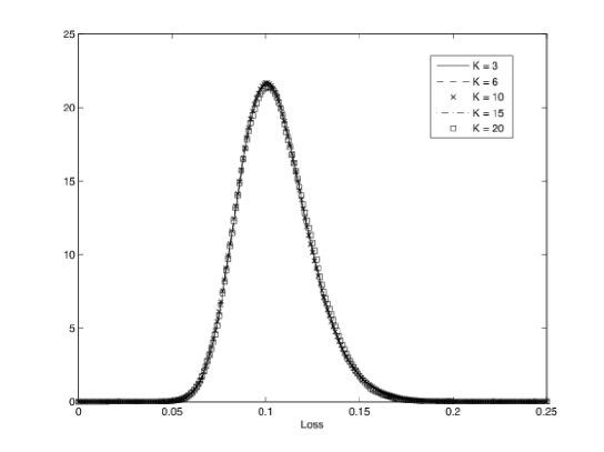
Figure 2 compares the approximate loss distribution according to (8) for different truncation levels K𝐾K of the fluctuation moment system (10). We use a time step of 0.0050.0050.005 and produce samples from X𝑋X using an Euler scheme. The approximate loss distribution converges very rapidly in terms of the truncation level. This conforms with previous numerical studies of the LLN moment system (9) which also demonstrated its quick convergence rate; see \citeasnounGieseckeSpiliopoulosSowersSirigano2012.

Refer to caption
Figure 2. Comparison of approximate loss distribution for different truncation levels at T=0.5𝑇0.5T=0.5. Parameter case is σ=0.9,α=4,λ0=λ¯=0.2,βC=1,formulae-sequenceformulae-sequence𝜎0.9formulae-sequence𝛼4subscript𝜆0¯𝜆0.2superscript𝛽𝐶1\sigma=0.9,\alpha=4,\lambda_{0}=\bar{\lambda}=0.2,\beta^{C}=1, and βS=1superscript𝛽𝑆1\beta^{S}=1. The systematic risk X𝑋X is an OU process with mean 111, reversion speed 222, volatility 111, and initial value 111. Approximate loss distribution computed using the conditionally semi-analytic Scheme 2. The fluctuation moments are truncated at level K𝐾K and the LLN moments are truncated at level 3K3𝐾3K.

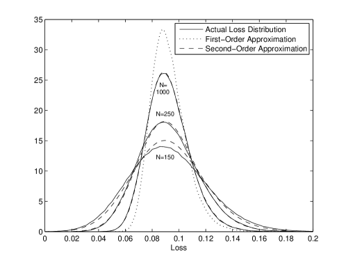
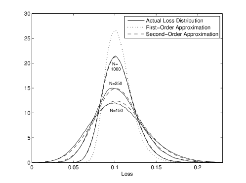
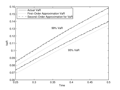
We now study the validity of the second-order approximation (8) by comparing it against the actual loss distribution from simulating the true finite system. In the following numerical studies, we choose a time step of 0.0050.0050.005 and a truncation level of K=6𝐾6K=6 for both schemes described above. A time step of 0.0050.0050.005 is used for simulating the finite system. Samples from X𝑋X are produced using an Euler scheme. Figure 3 compares the approximate loss distribution according to (8) with the actual loss distribution for βC=0superscript𝛽𝐶0\beta^{C}=0 and βS=1superscript𝛽𝑆1\beta^{S}=1, for each of several portfolio sizes. The approximate loss distribution is extremely accurate, even for a very small pool with only N=250𝑁250N=250. We also observe that the approximation accurately captures the tails of the actual loss distribution. Figure 4 compares the approximate loss distribution with the actual loss distribution for βC=1superscript𝛽𝐶1\beta^{C}=1 and βS=1superscript𝛽𝑆1\beta^{S}=1. The approximate loss distribution is again accurate, although not as accurate as when βC=0superscript𝛽𝐶0\beta^{C}=0. We also show in both Figures 3 and 4 the first-order LLN approximation (4). It is clear that the second-order approximation has increased accuracy, especially for smaller portfolios and in the tail of the distribution. Finally, Figure 5 shows a comparison for the 959595 and 999999 percent value at risk (VaR) between the actual loss, LLN approximation (4), and approximation (8) for a pool of N=1,000𝑁1000N=1,000. The approximation for the VaR based on (8) is significantly more accurate than the LLN approximation for the VaR.

Refer to caption
Figure 3. Comparison of approximate loss distribution and actual loss distribution in the finite system at T=0.5𝑇0.5T=0.5. Parameter case is σ=0.9,α=4,λ0=λ¯=0.2,βC=0formulae-sequenceformulae-sequence𝜎0.9formulae-sequence𝛼4subscript𝜆0¯𝜆0.2superscript𝛽𝐶0\sigma=0.9,\alpha=4,\lambda_{0}=\bar{\lambda}=0.2,\beta^{C}=0, and βS=1superscript𝛽𝑆1\beta^{S}=1. The systematic risk X𝑋X is an OU process with mean 111, reversion speed 222, volatility 111, and initial value 111. Approximate loss distribution computed using the conditionally semi-analytic Scheme 2.
Refer to caption
Figure 4. Comparison of approximate loss distribution and actual loss distribution in the finite system at T=0.5𝑇0.5T=0.5. Parameter case is σ=0.9,α=4,λ0=λ¯=0.2,βC=1,formulae-sequenceformulae-sequence𝜎0.9formulae-sequence𝛼4subscript𝜆0¯𝜆0.2superscript𝛽𝐶1\sigma=0.9,\alpha=4,\lambda_{0}=\bar{\lambda}=0.2,\beta^{C}=1, and βS=1superscript𝛽𝑆1\beta^{S}=1. The systematic risk X𝑋X is an OU process with mean 111, reversion speed 222, volatility 111, and initial value 111. Approximate loss distribution computed using the conditionally semi-analytic Scheme 2.
Refer to caption
Figure 5. Comparison of approximate and actual value at risks for N=1,000𝑁1000N=1,000. Parameter case is σ=0.9,α=4,λ0=λ¯=0.2,βC=1,formulae-sequenceformulae-sequence𝜎0.9formulae-sequence𝛼4subscript𝜆0¯𝜆0.2superscript𝛽𝐶1\sigma=0.9,\alpha=4,\lambda_{0}=\bar{\lambda}=0.2,\beta^{C}=1, and βS=1superscript𝛽𝑆1\beta^{S}=1. The systematic risk X𝑋X is an OU process with mean 111, reversion speed 222, volatility 111, and initial value 111. Approximate loss distribution computed using the conditionally semi-analytic Scheme 2.

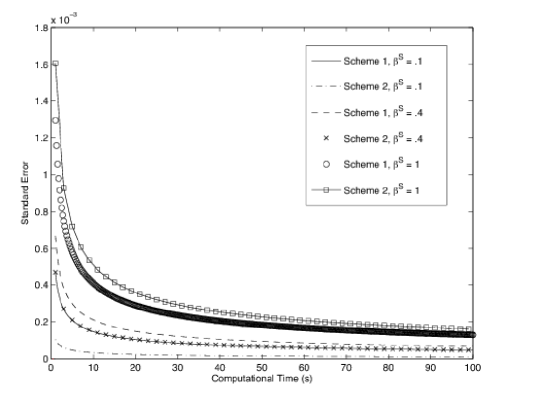
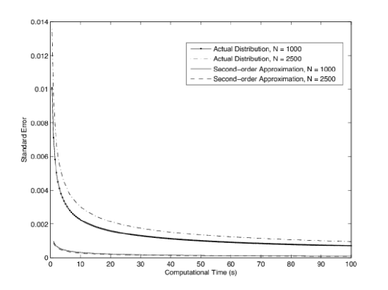
Appendix A provides additional numerical results on the performance of the numerical schemes. In particular, we demonstrate the advantages of the second-order approximation over direct simulation of the finite system (1). For a fixed computational time, the standard error for the second-order approximation is several orders of magnitude smaller than the standard error for the finite system simulation.

5.4. Approximate Loss Process

One of the significant advantages of the fluctuation analysis presented here is the dynamic approximation it provides for the entire loss process. An approximation of the loss process may be used to estimate the probability that the loss per month never exceeds a certain amount, or the density of the hitting time for the loss exceeding a certain level.

One can generate a sample skeleton of the approximate loss process according to the right hand side of (8) using Scheme 1. Although Scheme 2 gives the loss distribution at all time horizons, it does not directly yield a skeleton of the approximate loss process. However, due to the process being conditionally Gaussian, one can use a slightly modified form of Scheme 2 to simulate such a skeleton on as fine a time grid as desired. For small βSsuperscript𝛽𝑆\beta^{S}, one can expect that Scheme 222 will be more computationally efficient than Scheme 111 (see Appendix A for numerical results).

To simulate skeletons for the moments (10) of the fluctuation limit, one can use the following method. Let 𝐯0=0subscript𝐯00\mathbf{v}_{0}=0 (the general case is very similar). As usual, begin by simulating a path from the systematic risk process X𝑋X. Given a path of X𝑋X, we then simulate the loss at t=T𝑡𝑇t=T from the conditionally Gaussian distribution given by the formula (13). To simulate at 0<s<T0𝑠𝑇0<s<T, we only need the covariance matrix Cov[𝐯T,𝐯s|𝒱T]Covsubscript𝐯𝑇conditionalsubscript𝐯𝑠subscript𝒱𝑇\textrm{Cov}[\mathbf{v}_{T},\mathbf{v}_{s}|\mathcal{V}_{T}]. One can continue to simulate at grid points of one’s choice. For instance, one can simulate at time s1subscript𝑠1s_{1} where s<s1<T𝑠subscript𝑠1𝑇s<s_{1}<T given the covariance matrices Cov[𝐯T,𝐯s|𝒱T]Covsubscript𝐯𝑇conditionalsubscript𝐯𝑠subscript𝒱𝑇\textrm{Cov}[\mathbf{v}_{T},\mathbf{v}_{s}|\mathcal{V}_{T}], Cov[𝐯T,𝐯s1|𝒱T]Covsubscript𝐯𝑇conditionalsubscript𝐯subscript𝑠1subscript𝒱𝑇\textrm{Cov}[\mathbf{v}_{T},\mathbf{v}_{s_{1}}|\mathcal{V}_{T}], and Cov[𝐯s,𝐯s1|𝒱T]Covsubscript𝐯𝑠conditionalsubscript𝐯subscript𝑠1subscript𝒱𝑇\textrm{Cov}[\mathbf{v}_{s},\mathbf{v}_{s_{1}}|\mathcal{V}_{T}]. These covariance matrices are easily computed using the fundamental solution (16):

Σ(τ1,τ2)=Cov[𝐯τ1,𝐯τ2|𝒱T]=Ψ(τ1)[0τ1τ2Ψ1(s)Σ(s)(Ψ1(s))𝑑s]Ψ(τ2).Σsubscript𝜏1subscript𝜏2Covsubscript𝐯subscript𝜏1conditionalsubscript𝐯subscript𝜏2subscript𝒱𝑇Ψsubscript𝜏1delimited-[]superscriptsubscript0subscript𝜏1subscript𝜏2superscriptΨ1𝑠subscriptΣ𝑠superscriptsuperscriptΨ1𝑠topdifferential-d𝑠Ψsuperscriptsubscript𝜏2top\displaystyle\Sigma(\tau_{1},\tau_{2})=\textrm{Cov}[\mathbf{v}_{\tau_{1}},\mathbf{v}_{\tau_{2}}|\mathcal{V}_{T}]=\Psi(\tau_{1})\big{[}\int_{0}^{\tau_{1}\wedge\tau_{2}}\Psi^{-1}(s)\Sigma_{\mathcal{M}}(s)\big{(}\Psi^{-1}(s)\big{)}^{\top}ds\big{]}\Psi(\tau_{2})^{\top}.

To simulate 𝐯ssubscript𝐯𝑠\mathbf{v}_{s} given 𝐯τ1subscript𝐯subscript𝜏1\mathbf{v}_{\tau_{1}} and 𝐯τ2subscript𝐯subscript𝜏2\mathbf{v}_{\tau_{2}} where τ1<s<τ2subscript𝜏1𝑠subscript𝜏2\tau_{1}<s<\tau_{2}, we generate a sample from the multivariate Gaussian distribution 𝒩(μ~,Σ~)𝒩~𝜇~Σ\mathcal{N}(\tilde{\mu},\tilde{\Sigma}) where μ~=Σ1Σ21𝐙~𝜇subscriptΣ1superscriptsubscriptΣ21𝐙\tilde{\mu}=\Sigma_{1}\Sigma_{2}^{-1}\mathbf{Z} and Σ~=Σ(s,s)Σ1Σ21Σ1~ΣΣ𝑠𝑠subscriptΣ1superscriptsubscriptΣ21subscriptΣ1\tilde{\Sigma}=\Sigma(s,s)-\Sigma_{1}\Sigma_{2}^{-1}\Sigma_{1}. The matrices Σ1,Σ2,subscriptΣ1subscriptΣ2\Sigma_{1},\Sigma_{2}, and 𝐙𝐙\mathbf{Z} are

Σ1subscriptΣ1\displaystyle\Sigma_{1} =[Σ(s,τ1)Σ(s,τ2)]absentmatrixΣ𝑠subscript𝜏1Σ𝑠subscript𝜏2\displaystyle=\begin{bmatrix}\Sigma(s,\tau_{1})&\Sigma(s,\tau_{2})\end{bmatrix}
Σ2subscriptΣ2\displaystyle\Sigma_{2} =[Σ(τ1,τ1)Σ(τ1,τ2)Σ(τ1,τ2)Σ(τ2,τ2)]absentmatrixΣsubscript𝜏1subscript𝜏1Σsubscript𝜏1subscript𝜏2Σsubscript𝜏1subscript𝜏2Σsubscript𝜏2subscript𝜏2\displaystyle=\begin{bmatrix}\Sigma(\tau_{1},\tau_{1})&\Sigma(\tau_{1},\tau_{2})\\ \Sigma(\tau_{1},\tau_{2})&\Sigma(\tau_{2},\tau_{2})\end{bmatrix}
𝐙𝐙\displaystyle\mathbf{Z} =[𝐯τ1𝐯τ2]absentmatrixsubscript𝐯subscript𝜏1subscript𝐯subscript𝜏2\displaystyle=\begin{bmatrix}\mathbf{v}_{\tau_{1}}\\ \mathbf{v}_{\tau_{2}}\end{bmatrix}

It is worthwhile to note that this scheme requires only a single computation of the fundamental solution Ψm(t)superscriptΨ𝑚𝑡\Psi^{m}(t) for each path Xmsuperscript𝑋𝑚X^{m}. Given Ψm(t)superscriptΨ𝑚𝑡\Psi^{m}(t) for 0tT0𝑡𝑇0\leq t\leq T, one can generate as many skeletons of the fluctuation moments as desired for that particular Xmsuperscript𝑋𝑚X^{m} via the aforementioned method. In contrast, Scheme 1 requires one to resolve the system of SDEs (10) for each new realization. In particular, this suggests that this scheme will be more efficient than Scheme 111 for small βSsuperscript𝛽𝑆\beta^{S}.

Once skeletons from the fluctuation limit have been simulated, skeletons of the approximate loss process can be produced by combining these fluctuation paths with the law of large numbers limit process given by (9) and using the approximation formula (8).

5.5. Nonhomogeneous Portfolio

The moment method can be extended to a nonhomogeneous portfolio. Define the moments vk(t,𝗉)=+λkΞ¯t(dλ,𝗉)subscript𝑣𝑘𝑡𝗉subscriptsuperscriptsuperscript𝜆𝑘subscript¯Ξ𝑡𝑑𝜆𝗉v_{k}(t,\mathsf{p})=\int_{\mathbb{R}^{+}}\lambda^{k}\bar{\Xi}_{t}(d\lambda,\mathsf{p}) and uk(t,𝗉)=+λkμ¯t(dλ,𝗉)subscript𝑢𝑘𝑡𝗉subscriptsuperscriptsuperscript𝜆𝑘subscript¯𝜇𝑡𝑑𝜆𝗉u_{k}(t,\mathsf{p})=\int_{\mathbb{R}^{+}}\lambda^{k}\bar{\mu}_{t}(d\lambda,\mathsf{p}). Then

dvk(t,𝗉)𝑑subscript𝑣𝑘𝑡𝗉\displaystyle dv_{k}(t,\mathsf{p}) =βCkuk1(s,𝗉)(𝒫v1(t,𝗉)𝑑𝗉)dt+[12σ2k(k1)+αλ¯k+kβC𝒫u1(s,𝗉)𝑑𝗉]vk1(t,𝗉)dtabsentsuperscript𝛽𝐶𝑘subscript𝑢𝑘1𝑠𝗉subscript𝒫subscript𝑣1𝑡𝗉differential-d𝗉𝑑𝑡delimited-[]12superscript𝜎2𝑘𝑘1𝛼¯𝜆𝑘𝑘superscript𝛽𝐶subscript𝒫subscript𝑢1𝑠𝗉differential-d𝗉subscript𝑣𝑘1𝑡𝗉𝑑𝑡\displaystyle=\beta^{C}ku_{k-1}(s,\mathsf{p})\left(\int_{\mathcal{P}}v_{1}(t,\mathsf{p})d\mathsf{p}\right)dt+\left[\frac{1}{2}\sigma^{2}k(k-1)+\alpha\bar{\lambda}k+k\beta^{C}\int_{\mathcal{P}}u_{1}(s,\mathsf{p})d\mathsf{p}\right]v_{k-1}(t,\mathsf{p})dt
+vk(t,𝗉)[kα+kβSb0(Xt)+12k(k1)(βSσ0(Xt))2]dtvk+1(t,𝗉)dtsubscript𝑣𝑘𝑡𝗉delimited-[]𝑘𝛼𝑘superscript𝛽𝑆subscript𝑏0subscript𝑋𝑡12𝑘𝑘1superscriptsuperscript𝛽𝑆subscript𝜎0subscript𝑋𝑡2𝑑𝑡subscript𝑣𝑘1𝑡𝗉𝑑𝑡\displaystyle+v_{k}(t,\mathsf{p})\left[-k\alpha+k\beta^{S}b_{0}(X_{t})+\frac{1}{2}k(k-1)\left(\beta^{S}\sigma_{0}(X_{t})\right)^{2}\right]dt-v_{k+1}(t,\mathsf{p})dt
+kβSσ0(Xt)vk(t,𝗉)dVt+¯k(t,𝗉),𝑘superscript𝛽𝑆subscript𝜎0subscript𝑋𝑡subscript𝑣𝑘𝑡𝗉𝑑subscript𝑉𝑡subscript¯𝑘𝑡𝗉\displaystyle+k\beta^{S}\sigma_{0}(X_{t})v_{k}(t,\mathsf{p})dV_{t}+\bar{\mathcal{M}}_{k}(t,\mathsf{p}),
vk(0,𝗉)subscript𝑣𝑘0𝗉\displaystyle v_{k}(0,\mathsf{p}) =0λkΞ¯0(dλ,𝗉).absentsuperscriptsubscript0superscript𝜆𝑘subscript¯Ξ0𝑑𝜆𝗉\displaystyle=\int_{0}^{\infty}\lambda^{k}\bar{\Xi}_{0}(d\lambda,\mathsf{p}).

The covariation [d¯k(t,𝗉1),d¯j(t,𝗉2)]𝑑subscript¯𝑘𝑡subscript𝗉1𝑑subscript¯𝑗𝑡subscript𝗉2\big{[}d\bar{\mathcal{M}}_{k}(t,\mathsf{p}_{1}),d\bar{\mathcal{M}}_{j}(t,\mathsf{p}_{2})\big{]} for 𝗉1,𝗉2subscript𝗉1subscript𝗉2\mathsf{p}_{1},\mathsf{p}_{2} \in 𝒫𝒫\mathcal{P} is given by

[d¯k(t,𝗉1),d¯j(t,𝗉2)]𝑑subscript¯𝑘𝑡subscript𝗉1𝑑subscript¯𝑗𝑡subscript𝗉2\displaystyle\big{[}d\bar{\mathcal{M}}_{k}(t,\mathsf{p}_{1}),d\bar{\mathcal{M}}_{j}(t,\mathsf{p}_{2})\big{]} =𝟏𝗉1=𝗉2(σ2kjuk+j1(t,𝗉1)+uk+j+1(t,𝗉1)βCkuk1(t,𝗉1)uj+1(t,𝗉1)\displaystyle=\mathbf{1}_{\mathsf{p}_{1}=\mathsf{p}_{2}}\big{(}\sigma^{2}kju_{k+j-1}(t,\mathsf{p}_{1})+u_{k+j+1}(t,\mathsf{p}_{1})-\beta^{C}ku_{k-1}(t,\mathsf{p}_{1})u_{j+1}(t,\mathsf{p}_{1})
βCjuj1(t,𝗉1)uk+1(t,𝗉1)+(βC)2kjuk1(t,𝗉1)uj1(t,𝗉1)u1(t,𝗉1))dt.\displaystyle-\beta^{C}ju_{j-1}(t,\mathsf{p}_{1})u_{k+1}(t,\mathsf{p}_{1})+(\beta^{C})^{2}kju_{k-1}(t,\mathsf{p}_{1})u_{j-1}(t,\mathsf{p}_{1})u_{1}(t,\mathsf{p}_{1})\big{)}dt.

The LLN moments are

duk(t,𝗉)𝑑subscript𝑢𝑘𝑡𝗉\displaystyle du_{k}(t,\mathsf{p}) =uk(t,𝗉)[αk+βSb0(Xt)k+12(βS)2σ02(Xt)k(k1)]dtuk+1(t,𝗉)dtabsentsubscript𝑢𝑘𝑡𝗉delimited-[]𝛼𝑘superscript𝛽𝑆subscript𝑏0subscript𝑋𝑡𝑘12superscriptsuperscript𝛽𝑆2superscriptsubscript𝜎02subscript𝑋𝑡𝑘𝑘1𝑑𝑡subscript𝑢𝑘1𝑡𝗉𝑑𝑡\displaystyle=u_{k}(t,\mathsf{p})\left[-\alpha k+\beta^{S}b_{0}(X_{t})k+\frac{1}{2}(\beta^{S})^{2}\sigma_{0}^{2}(X_{t})k(k-1)\right]dt-u_{k+1}(t,\mathsf{p})dt
+uk1(t,𝗉)[0.5σ2k(k1)+αλ¯k+βCk𝒫u1(t,𝗉)𝑑𝗉]dt+βSσ0(Xt)kuk(t,𝗉)dVtsubscript𝑢𝑘1𝑡𝗉delimited-[]0.5superscript𝜎2𝑘𝑘1𝛼¯𝜆𝑘superscript𝛽𝐶𝑘subscript𝒫subscript𝑢1𝑡𝗉differential-d𝗉𝑑𝑡superscript𝛽𝑆subscript𝜎0subscript𝑋𝑡𝑘subscript𝑢𝑘𝑡𝗉𝑑subscript𝑉𝑡\displaystyle+u_{k-1}(t,\mathsf{p})\left[0.5\sigma^{2}k(k-1)+\alpha\bar{\lambda}k+\beta^{C}k\int_{\mathcal{P}}u_{1}(t,\mathsf{p})d\mathsf{p}\right]dt+\beta^{S}\sigma_{0}(X_{t})ku_{k}(t,\mathsf{p})dV_{t}
uk(0,𝗉)subscript𝑢𝑘0𝗉\displaystyle u_{k}(0,\mathsf{p}) =0λkμ¯0(dλ,𝗉).absentsuperscriptsubscript0superscript𝜆𝑘subscript¯𝜇0𝑑𝜆𝗉\displaystyle=\int_{0}^{\infty}\lambda^{k}\bar{\mu}_{0}(d\lambda,\mathsf{p}).

For numerical implementation, one must discretize the parameter space 𝒫𝒫\mathcal{P}. As we allow more parameters to vary, 𝒫𝒫\mathcal{P} can become high dimensional. This can become computationally expensive.

6. Proof of Theorem 4.1

In this section we prove the fluctuation Theorem 4.1. The methodology of the proof goes as follows. After some preliminary computations, we obtain a convenient formulation of the equation that {ΞtN}subscriptsuperscriptΞ𝑁𝑡\{\Xi^{N}_{t}\} satisfies, see (20). Some terms in this equation will vanish in the limit as N𝑁N\rightarrow\infty; this is Lemma 6.1. Based on tightness of the involved processes (the topic of Section 8) and continuity properties of the operators involved, we can then pass to the limit and thus identify the limiting equation. The limit process satisfies in the weak form another stochastic evolution, which has a unique solution (proven in Section 9). The difficulty is to identify a rich enough space where tightness and uniqueness can be simultaneously proven. This is not trivial in our case, because the coefficients are not bounded and the equation degenerates (coefficients of the highest derivatives are not bounded away from zero). It turns out that the appopriate space in which one can prove both tightness and uniqueness is a weighted Sobolev space, introduced in \citeasnounPurtukhia1984 and further generalized in \citeasnounGyongiKrylov1992 to study stochastic partial differential equations with unbounded coefficients, and are briefly reviewed in Section 7.

An application of Itô’s formula shows that for fCb2(𝒫^)𝑓subscriptsuperscript𝐶2𝑏^𝒫f\in C^{2}_{b}(\hat{\mathcal{P}}),

f,μtNEsubscript𝑓subscriptsuperscript𝜇𝑁𝑡𝐸\displaystyle\left\langle f,\mu^{N}_{t}\right\rangle_{E} =f,μ0NE+0t{1f,μsNE+𝒬,μsNE2f,μsNE+3Xsf,μsNE}𝑑sabsentsubscript𝑓subscriptsuperscript𝜇𝑁0𝐸superscriptsubscript0𝑡subscriptsubscript1𝑓subscriptsuperscript𝜇𝑁𝑠𝐸subscript𝒬subscriptsuperscript𝜇𝑁𝑠𝐸subscriptsubscript2𝑓subscriptsuperscript𝜇𝑁𝑠𝐸subscriptsubscriptsuperscriptsubscript𝑋𝑠3𝑓subscriptsuperscript𝜇𝑁𝑠𝐸differential-d𝑠\displaystyle=\left\langle f,\mu^{N}_{0}\right\rangle_{E}+\int_{0}^{t}\left\{\left\langle\mathcal{L}_{1}f,\mu^{N}_{s}\right\rangle_{E}+\left\langle\mathcal{Q},\mu^{N}_{s}\right\rangle_{E}\left\langle\mathcal{L}_{2}f,\mu^{N}_{s}\right\rangle_{E}+\left\langle\mathcal{L}^{X_{s}}_{3}f,\mu^{N}_{s}\right\rangle_{E}\right\}ds
(18) +0tA^N[f](Xs,μsN)𝑑s+0t4Xsf,μsNE𝑑Vs+f,tNsuperscriptsubscript0𝑡superscript^𝐴𝑁delimited-[]𝑓subscript𝑋𝑠subscriptsuperscript𝜇𝑁𝑠differential-d𝑠superscriptsubscript0𝑡subscriptsuperscriptsubscript4subscript𝑋𝑠𝑓subscriptsuperscript𝜇𝑁𝑠𝐸differential-dsubscript𝑉𝑠𝑓subscriptsuperscript𝑁𝑡\displaystyle+\int_{0}^{t}\hat{A}^{N}[f](X_{s},\mu^{N}_{s})ds+\int_{0}^{t}\left\langle\mathcal{L}_{4}^{X_{s}}f,\mu^{N}_{s}\right\rangle_{E}dV_{s}+\left\langle f,\mathcal{M}^{N}_{t}\right\rangle

where

𝒜^N[f](Xs,μsN)=n=1NλsN,n𝒥N,nf(s)msN,n{𝒬,μsNE2f,μsNEf,μsNE},superscript^𝒜𝑁delimited-[]𝑓subscript𝑋𝑠subscriptsuperscript𝜇𝑁𝑠superscriptsubscript𝑛1𝑁subscriptsuperscript𝜆𝑁𝑛𝑠subscriptsuperscript𝒥𝑓𝑁𝑛𝑠subscriptsuperscriptm𝑁𝑛𝑠subscript𝒬subscriptsuperscript𝜇𝑁𝑠𝐸subscriptsubscript2𝑓subscriptsuperscript𝜇𝑁𝑠𝐸subscript𝑓subscriptsuperscript𝜇𝑁𝑠𝐸\hat{\mathcal{A}}^{N}[f](X_{s},\mu^{N}_{s})=\sum_{n=1}^{N}\lambda^{N,n}_{s}\mathcal{J}^{f}_{N,n}(s)\textsc{m}^{N,n}_{s}-\left\{\left\langle\mathcal{Q},\mu^{N}_{s}\right\rangle_{E}\left\langle\mathcal{L}_{2}f,\mu^{N}_{s}\right\rangle_{E}-\left\langle f,\mu^{N}_{s}\right\rangle_{E}\right\},
𝒥N,nf(s)=1Nn=1N{f(𝗉N,n,λsN,n+βN,nCN)f(𝗉N,n,λsN,n)}msN,n1Nf(𝗉N,n,λsN,n)subscriptsuperscript𝒥𝑓𝑁𝑛𝑠1𝑁superscriptsubscriptsuperscript𝑛1𝑁𝑓superscript𝗉𝑁superscript𝑛subscriptsuperscript𝜆𝑁superscript𝑛𝑠subscriptsuperscript𝛽𝐶𝑁superscript𝑛𝑁𝑓superscript𝗉𝑁superscript𝑛subscriptsuperscript𝜆𝑁superscript𝑛𝑠subscriptsuperscriptm𝑁superscript𝑛𝑠1𝑁𝑓superscript𝗉𝑁𝑛subscriptsuperscript𝜆𝑁𝑛𝑠\mathcal{J}^{f}_{N,n}(s)=\frac{1}{N}\sum_{n^{\prime}=1}^{N}\left\{f\left(\mathsf{p}^{N,n^{\prime}},\lambda^{N,n^{\prime}}_{s}+\frac{\beta^{C}_{N,n^{\prime}}}{N}\right)-f\left(\mathsf{p}^{N,n^{\prime}},\lambda^{N,n^{\prime}}_{s}\right)\right\}\textsc{m}^{N,n^{\prime}}_{s}-\frac{1}{N}f\left(\mathsf{p}^{N,n},\lambda^{N,n}_{s}\right)

for all s0𝑠0s\geq 0, N𝑁N\in\mathbb{N} and n{1,2,,N}𝑛12𝑁n\in\{1,2,\dots,N\},

f,tN=1Nn=1N0tσN,nλtN,nfλ(𝗉^sN,n)msN,n𝑑Wsn+n=1N0t𝒥N,nf(s)𝑑𝒩sN,n𝑓subscriptsuperscript𝑁𝑡1𝑁superscriptsubscript𝑛1𝑁superscriptsubscript0𝑡subscript𝜎𝑁𝑛superscriptsubscript𝜆𝑡𝑁𝑛𝑓𝜆subscriptsuperscript^𝗉𝑁𝑛𝑠subscriptsuperscriptm𝑁𝑛𝑠differential-dsubscriptsuperscript𝑊𝑛𝑠superscriptsubscript𝑛1𝑁superscriptsubscript0𝑡subscriptsuperscript𝒥𝑓𝑁𝑛𝑠differential-dsubscriptsuperscript𝒩𝑁𝑛𝑠\left\langle f,\mathcal{M}^{N}_{t}\right\rangle=\frac{1}{N}\sum_{n=1}^{N}\int_{0}^{t}\sigma_{{N,n}}\sqrt{\lambda_{t}^{{N,n}}}\frac{\partial f}{\partial\lambda}(\hat{\mathsf{p}}^{{N,n}}_{s})\textsc{m}^{N,n}_{s}dW^{n}_{s}+\sum_{n=1}^{N}\int_{0}^{t}\mathcal{J}^{f}_{N,n}(s)d\mathcal{N}^{{N,n}}_{s}

and

𝒩sN,n=(1msN,n)0sλrN,nmrN,n𝑑r.subscriptsuperscript𝒩𝑁𝑛𝑠1subscriptsuperscriptm𝑁𝑛𝑠superscriptsubscript0𝑠subscriptsuperscript𝜆𝑁𝑛𝑟subscriptsuperscriptm𝑁𝑛𝑟differential-d𝑟\mathcal{N}^{{N,n}}_{s}=(1-\textsc{m}^{N,n}_{s})-\int_{0}^{s}\lambda^{N,n}_{r}\textsc{m}^{N,n}_{r}dr.

By subtracting (3) from (18) we find that ΞtNsubscriptsuperscriptΞ𝑁𝑡\Xi^{N}_{t} satisfies the equation

f,ΞtN𝑓subscriptsuperscriptΞ𝑁𝑡\displaystyle\left\langle f,\Xi^{N}_{t}\right\rangle =f,Ξ0N+0t1f+3Xsf,ΞsN𝑑s+0t[𝒬,μ¯s2f,ΞsN+𝒬,ΞsN2f,μsN]𝑑sabsent𝑓subscriptsuperscriptΞ𝑁0superscriptsubscript0𝑡subscript1𝑓subscriptsuperscriptsubscript𝑋𝑠3𝑓subscriptsuperscriptΞ𝑁𝑠differential-d𝑠superscriptsubscript0𝑡delimited-[]𝒬subscript¯𝜇𝑠subscript2𝑓subscriptsuperscriptΞ𝑁𝑠𝒬subscriptsuperscriptΞ𝑁𝑠subscript2𝑓subscriptsuperscript𝜇𝑁𝑠differential-d𝑠\displaystyle=\left\langle f,\Xi^{N}_{0}\right\rangle+\int_{0}^{t}\left\langle\mathcal{L}_{1}f+\mathcal{L}^{X_{s}}_{3}f,\Xi^{N}_{s}\right\rangle ds+\int_{0}^{t}\left[\left\langle\mathcal{Q},\bar{\mu}_{s}\right\rangle\left\langle\mathcal{L}_{2}f,\Xi^{N}_{s}\right\rangle+\left\langle\mathcal{Q},\Xi^{N}_{s}\right\rangle\left\langle\mathcal{L}_{2}f,\mu^{N}_{s}\right\rangle\right]ds
+0tNA^N[f](Xs,μsN)𝑑s+0t4Xsf,ΞsN𝑑Vs+f,NtN.superscriptsubscript0𝑡𝑁superscript^𝐴𝑁delimited-[]𝑓subscript𝑋𝑠subscriptsuperscript𝜇𝑁𝑠differential-d𝑠superscriptsubscript0𝑡subscriptsuperscriptsubscript𝑋𝑠4𝑓subscriptsuperscriptΞ𝑁𝑠differential-dsubscript𝑉𝑠𝑓𝑁subscriptsuperscript𝑁𝑡\displaystyle+\int_{0}^{t}\sqrt{N}\hat{A}^{N}[f](X_{s},\mu^{N}_{s})ds+\int_{0}^{t}\left\langle\mathcal{L}^{X_{s}}_{4}f,\Xi^{N}_{s}\right\rangle dV_{s}+\left\langle f,\sqrt{N}\mathcal{M}^{N}_{t}\right\rangle.

In order to simplify the calculations later on, for each fCb2(𝒫^)𝑓subscriptsuperscript𝐶2𝑏^𝒫f\in C^{2}_{b}(\hat{\mathcal{P}}), t0𝑡0t\geq 0, N𝑁N\in\mathbb{N} and n{1,2,,N}𝑛12𝑁n\in\{1,2,\dots,N\}, we define the quantity

𝒥~N,nf(t)=def1Nm=1NβN,mCfλ(𝗉^tN,m)mtN,mf(𝗉N,n,λtN,n)=2f,μtNEf(𝗉^tN).subscriptsuperscript~𝒥𝑓𝑁𝑛𝑡def1𝑁superscriptsubscript𝑚1𝑁subscriptsuperscript𝛽𝐶𝑁𝑚𝑓𝜆subscriptsuperscript^𝗉𝑁𝑚𝑡subscriptsuperscriptm𝑁𝑚𝑡𝑓superscript𝗉𝑁𝑛subscriptsuperscript𝜆𝑁𝑛𝑡subscriptsubscript2𝑓subscriptsuperscript𝜇𝑁𝑡𝐸𝑓subscriptsuperscript^𝗉𝑁𝑡\tilde{\mathcal{J}}^{f}_{N,n}(t)\overset{\text{def}}{=}\frac{1}{N}\sum_{m=1}^{N}\beta^{C}_{N,m}\frac{\partial f}{\partial\lambda}(\hat{\mathsf{p}}^{N,m}_{t})\textsc{m}^{N,m}_{t}-f\left(\mathsf{p}^{N,n},\lambda^{N,n}_{t}\right)=\left\langle\mathcal{L}_{2}f,\mu^{N}_{t}\right\rangle_{E}-f(\hat{\mathsf{p}}^{N}_{t}).

A simple computation shows that

(19) |𝒥N,nf(t)1N𝒥~N,nf(t)|K2N22fλ2C.subscriptsuperscript𝒥𝑓𝑁𝑛𝑡1𝑁subscriptsuperscript~𝒥𝑓𝑁𝑛𝑡superscript𝐾2superscript𝑁2subscriptnormsuperscript2𝑓superscript𝜆2𝐶\left|\mathcal{J}^{f}_{N,n}(t)-\frac{1}{N}\tilde{\mathcal{J}}^{f}_{N,n}(t)\right|\leq\frac{K^{2}}{N^{2}}\left\|\frac{\partial^{2}f}{\partial\lambda^{2}}\right\|_{C}.

We can rewrite the stochastic evolution equation that ΞNsuperscriptΞ𝑁\Xi^{N} satisfies as follows:

(20) f,ΞtN𝑓subscriptsuperscriptΞ𝑁𝑡\displaystyle\left\langle f,\Xi^{N}_{t}\right\rangle =\displaystyle= f,Ξ0N+0t1f+3Xtf,ΞsN𝑑s+0t[𝒬,μ¯s2f,ΞsN+𝒬,ΞsN2f,μsN]𝑑s𝑓subscriptsuperscriptΞ𝑁0superscriptsubscript0𝑡subscript1𝑓subscriptsuperscriptsubscript𝑋𝑡3𝑓subscriptsuperscriptΞ𝑁𝑠differential-d𝑠superscriptsubscript0𝑡delimited-[]𝒬subscript¯𝜇𝑠subscript2𝑓subscriptsuperscriptΞ𝑁𝑠𝒬subscriptsuperscriptΞ𝑁𝑠subscript2𝑓subscriptsuperscript𝜇𝑁𝑠differential-d𝑠\displaystyle\left\langle f,\Xi^{N}_{0}\right\rangle+\int_{0}^{t}\left\langle\mathcal{L}_{1}f+\mathcal{L}^{X_{t}}_{3}f,\Xi^{N}_{s}\right\rangle ds+\int_{0}^{t}\left[\left\langle\mathcal{Q},\bar{\mu}_{s}\right\rangle\left\langle\mathcal{L}_{2}f,\Xi^{N}_{s}\right\rangle+\left\langle\mathcal{Q},\Xi^{N}_{s}\right\rangle\left\langle\mathcal{L}_{2}f,\mu^{N}_{s}\right\rangle\right]ds
+\displaystyle+ 0t4Xsf,ΞsN𝑑Vs+f,N~tN+Rt,0Nsuperscriptsubscript0𝑡subscriptsuperscriptsubscript𝑋𝑠4𝑓subscriptsuperscriptΞ𝑁𝑠differential-dsubscript𝑉𝑠𝑓𝑁subscriptsuperscript~𝑁𝑡subscriptsuperscript𝑅𝑁𝑡0\displaystyle\int_{0}^{t}\left\langle\mathcal{L}^{X_{s}}_{4}f,\Xi^{N}_{s}\right\rangle dV_{s}+\left\langle f,\sqrt{N}\tilde{\mathcal{M}}^{N}_{t}\right\rangle+R^{N}_{t,0}

where

f,N~tN𝑓𝑁subscriptsuperscript~𝑁𝑡\displaystyle\left\langle f,\sqrt{N}\tilde{\mathcal{M}}^{N}_{t}\right\rangle =N(1Nn=1N0tσN,nλtN,nfλ(𝗉^sN,n)msN,n𝑑Wsn+1Nn=1N0t𝒥~N,nf(s)𝑑𝒩sN,n)absent𝑁1𝑁superscriptsubscript𝑛1𝑁superscriptsubscript0𝑡subscript𝜎𝑁𝑛superscriptsubscript𝜆𝑡𝑁𝑛𝑓𝜆subscriptsuperscript^𝗉𝑁𝑛𝑠subscriptsuperscriptm𝑁𝑛𝑠differential-dsubscriptsuperscript𝑊𝑛𝑠1𝑁superscriptsubscript𝑛1𝑁superscriptsubscript0𝑡subscriptsuperscript~𝒥𝑓𝑁𝑛𝑠differential-dsubscriptsuperscript𝒩𝑁𝑛𝑠\displaystyle=\sqrt{N}\left(\frac{1}{N}\sum_{n=1}^{N}\int_{0}^{t}\sigma_{{N,n}}\sqrt{\lambda_{t}^{{N,n}}}\frac{\partial f}{\partial\lambda}(\hat{\mathsf{p}}^{{N,n}}_{s})\textsc{m}^{N,n}_{s}dW^{n}_{s}+\frac{1}{N}\sum_{n=1}^{N}\int_{0}^{t}\tilde{\mathcal{J}}^{f}_{N,n}(s)d\mathcal{N}^{{N,n}}_{s}\right)
Rt,0Nsubscriptsuperscript𝑅𝑁𝑡0\displaystyle R^{N}_{t,0} =0tNA^N[f](Xs,μsN)𝑑s+n=1N0tNB^N,n[f](s)𝑑𝒩sN,nabsentsuperscriptsubscript0𝑡𝑁superscript^𝐴𝑁delimited-[]𝑓subscript𝑋𝑠subscriptsuperscript𝜇𝑁𝑠differential-d𝑠superscriptsubscript𝑛1𝑁superscriptsubscript0𝑡𝑁superscript^𝐵𝑁𝑛delimited-[]𝑓𝑠differential-dsubscriptsuperscript𝒩𝑁𝑛𝑠\displaystyle=\int_{0}^{t}\sqrt{N}\hat{A}^{N}[f](X_{s},\mu^{N}_{s})ds+\sum_{n=1}^{N}\int_{0}^{t}\sqrt{N}\hat{B}^{{N,n}}[f](s)d\mathcal{N}^{{N,n}}_{s}
B^N,n[f](s)superscript^𝐵𝑁𝑛delimited-[]𝑓𝑠\displaystyle\hat{B}^{{N,n}}[f](s) =𝒥N,nf(s)1N𝒥~N,nf(s).absentsubscriptsuperscript𝒥𝑓𝑁𝑛𝑠1𝑁subscriptsuperscript~𝒥𝑓𝑁𝑛𝑠\displaystyle=\mathcal{J}^{f}_{N,n}(s)-\frac{1}{N}\tilde{\mathcal{J}}^{f}_{N,n}(s).

The term Rt,0Nsubscriptsuperscript𝑅𝑁𝑡0R^{N}_{t,0} turns out to vanish in the limit as the following lemma shows.

Lemma 6.1.

For any t[0,T]𝑡0𝑇t\in[0,T] and any fCb2(𝒫^)𝑓subscriptsuperscript𝐶2𝑏^𝒫f\in C^{2}_{b}(\hat{\mathcal{P}}), there is a constant C0subscript𝐶0C_{0}, independent of n,N𝑛𝑁n,N such that

𝔼[0tN|𝒜^N[f](Xr,μrN)|𝑑r]C0Nt𝔼delimited-[]superscriptsubscript0𝑡𝑁superscript^𝒜𝑁delimited-[]𝑓subscript𝑋𝑟subscriptsuperscript𝜇𝑁𝑟differential-d𝑟subscript𝐶0𝑁𝑡\mathbb{E}\left[\int_{0}^{t}\sqrt{N}\left|\hat{\mathcal{A}}^{N}[f](X_{r},\mu^{N}_{r})\right|dr\right]\leq\frac{C_{0}}{\sqrt{N}}t

and

sup0tT𝔼[n=1N0tNB^N,n[f](s)𝑑𝒩sN,n]2C0N2T.subscriptsupremum0𝑡𝑇𝔼superscriptdelimited-[]superscriptsubscript𝑛1𝑁superscriptsubscript0𝑡𝑁superscript^𝐵𝑁𝑛delimited-[]𝑓𝑠differential-dsubscriptsuperscript𝒩𝑁𝑛𝑠2subscript𝐶0superscript𝑁2𝑇\sup_{0\leq t\leq T}\mathbb{E}\left[\sum_{n=1}^{N}\int_{0}^{t}\sqrt{N}\hat{B}^{{N,n}}[f](s)d\mathcal{N}^{{N,n}}_{s}\right]^{2}\leq\frac{C_{0}}{N^{2}}T.

Moreover, we have that

limN𝔼sup0tT|Rt,0N|2=0.subscript𝑁𝔼subscriptsupremum0𝑡𝑇superscriptsubscriptsuperscript𝑅𝑁𝑡020\lim_{N\rightarrow\infty}\mathbb{E}\sup_{0\leq t\leq T}|R^{N}_{t,0}|^{2}=0.

Lastly, regarding the conditional (on 𝒱tsubscript𝒱𝑡\mathcal{V}_{t}) covariation of the martingale term f,N~tN𝑓𝑁subscriptsuperscript~𝑁𝑡\left\langle f,\sqrt{N}\tilde{\mathcal{M}}^{N}_{t}\right\rangle we have

(21) Cov[f,N~t1N,g,N~t2N|𝒱t1t2]Cov𝑓𝑁subscriptsuperscript~𝑁subscript𝑡1conditional𝑔𝑁subscriptsuperscript~𝑁subscript𝑡2subscript𝒱subscript𝑡1subscript𝑡2\displaystyle\mathrm{Cov}\left[\left\langle f,\sqrt{N}\tilde{\mathcal{M}}^{N}_{t_{1}}\right\rangle,\left\langle g,\sqrt{N}\tilde{\mathcal{M}}^{N}_{t_{2}}\right\rangle\Big{|}\mathcal{V}_{t_{1}\vee t_{2}}\right] =\displaystyle= 𝔼[0t1t2[5(f,g),μsN+6(f,g),μsN+\displaystyle\mathbb{E}\left[\int_{0}^{t_{1}\wedge t_{2}}\left[\left\langle\mathcal{L}_{5}(f,g),\mu^{N}_{s}\right\rangle+\left\langle\mathcal{L}_{6}(f,g),\mu^{N}_{s}\right\rangle+\right.\right.
+2f,μsN2g,μsN𝒬,μsNlimit-fromsubscript2𝑓subscriptsuperscript𝜇𝑁𝑠subscript2𝑔subscriptsuperscript𝜇𝑁𝑠𝒬subscriptsuperscript𝜇𝑁𝑠\displaystyle\left.\left.+\left\langle\mathcal{L}_{2}f,\mu^{N}_{s}\right\rangle\left\langle\mathcal{L}_{2}g,\mu^{N}_{s}\right\rangle\left\langle\mathcal{Q},\mu^{N}_{s}\right\rangle-\right.\right.
7g,μsN2f,μsN7f,μsN2g,μsN]ds|𝒱t1t2].\displaystyle\left.\left.-\left\langle\mathcal{L}_{7}g,\mu^{N}_{s}\right\rangle\left\langle\mathcal{L}_{2}f,\mu^{N}_{s}\right\rangle-\left\langle\mathcal{L}_{7}f,\mu^{N}_{s}\right\rangle\left\langle\mathcal{L}_{2}g,\mu^{N}_{s}\right\rangle\right]ds\Big{|}\mathcal{V}_{t_{1}\vee t_{2}}\right].

We continue with the proof of the theorem and defer the proof of Lemma 6.1 to the end of this section. Relative compactness of the sequences {ΞtN,n,t[0,T]}NsubscriptsubscriptsuperscriptΞ𝑁𝑛𝑡𝑡0𝑇𝑁\left\{\Xi^{{N,n}}_{t},t\in[0,T]\right\}_{N\in\mathbb{N}} and {NM~tN,n,t[0,T]}Nsubscript𝑁subscriptsuperscript~𝑀𝑁𝑛𝑡𝑡0𝑇𝑁\left\{\sqrt{N}\tilde{M}^{{N,n}}_{t},t\in[0,T]\right\}_{N\in\mathbb{N}} in DW0J(w,ρ)[0,T]subscript𝐷subscriptsuperscript𝑊𝐽0𝑤𝜌0𝑇D_{W^{-J}_{0}(w,\rho)}[0,T] follows by Lemmas 8.7 and 8.8. Relative compactness of the sequence {μtN,t[0,T]}Nsubscriptsubscriptsuperscript𝜇𝑁𝑡𝑡0𝑇𝑁\left\{\mu^{N}_{t},t\in[0,T]\right\}_{N\in\mathbb{N}} in DE[0,T]subscript𝐷𝐸0𝑇D_{E}[0,T] follows by Lemma 7.1 in \citeasnounGieseckeSpiliopoulosSowersSirigano2012. These imply that the sequence

{(μN,N~N,ΞN,V),N}superscript𝜇𝑁𝑁superscript~𝑁superscriptΞ𝑁𝑉𝑁\left\{\left(\mu^{N},\sqrt{N}\tilde{\mathcal{M}}^{N},\Xi^{N},V\right),N\in\mathbb{N}\right\}

is relatively compact in DE×W0J(w,ρ)×W0J(w,ρ)×[0,T]subscript𝐷𝐸subscriptsuperscript𝑊𝐽0𝑤𝜌subscriptsuperscript𝑊𝐽0𝑤𝜌0𝑇D_{E\times W^{-J}_{0}(w,\rho)\times W^{-J}_{0}(w,\rho)\times\mathbb{R}}[0,T]. Let us denote by

{(μ¯,¯,Ξ¯,V)}¯𝜇¯¯Ξ𝑉\left\{\left(\bar{\mu},\bar{\mathcal{M}},\bar{\Xi},V\right)\right\}

a limit point of this sequence. We mention here that this is a limit in distribution, so the limit point may not be defined on the same probability space as the prelimit sequence, but nevertheless V𝑉V (and thus X𝑋X), have the same distribution both in the limit and in the prelimit. Then, by (20), Lemma 6.1 and the continuity of the operators 𝒢𝒢\mathcal{G} and 4subscript4\mathcal{L}_{4} we get that {(μ¯,¯,Ξ¯,V)}¯𝜇¯¯Ξ𝑉\left\{\left(\bar{\mu},\bar{\mathcal{M}},\bar{\Xi},V\right)\right\} will satisfy, due to Theorem 5.5 in \citeasnounKurtzProtter, the stochastic evolution equation (6). By Lemma 6.1, the conditional covariation of the distribution valued martingale ¯¯\bar{\mathcal{M}} is given by (7). Uniqueness follows by Theorem 9.7. This concludes the proof of the theorem.

We conclude this section with the proof of Lemma 6.1.

Proof of Lemma 6.1.

We start by recalling that Lemma 3.4 in \citeasnounGieseckeSpiliopoulosSowers2011 states that for each p1𝑝1p\geq 1 and T0𝑇0T\geq 0,

(22) sup0tTN1Nn=1N𝔼[|λtN,n|p]Csubscriptsupremum0𝑡𝑇𝑁1𝑁superscriptsubscript𝑛1𝑁𝔼delimited-[]superscriptsubscriptsuperscript𝜆𝑁𝑛𝑡𝑝𝐶\sup_{\begin{subarray}{c}0\leq t\leq T\\ N\in\mathbb{N}\end{subarray}}\frac{1}{N}\sum_{n=1}^{N}\mathbb{E}\left[|\lambda^{N,n}_{t}|^{p}\right]\leq C

for some constant C>0𝐶0C>0 that is independent of N,n𝑁𝑛{N,n}. Along with (19), this implies that

𝔼[0tN|𝒜^N[f](Xr,μrN)|𝑑r]𝔼delimited-[]superscriptsubscript0𝑡𝑁superscript^𝒜𝑁delimited-[]𝑓subscript𝑋𝑟subscriptsuperscript𝜇𝑁𝑟differential-d𝑟\displaystyle\mathbb{E}\left[\int_{0}^{t}\sqrt{N}\left|\hat{\mathcal{A}}^{N}[f](X_{r},\mu^{N}_{r})\right|dr\right] =𝔼[0tN|n=1NλrN,n𝒥N,nf(r)mrN,n1Nn=1NλrN,n𝒥~N,nf(r)mrN,n|𝑑r]absent𝔼delimited-[]superscriptsubscript0𝑡𝑁superscriptsubscript𝑛1𝑁subscriptsuperscript𝜆𝑁𝑛𝑟subscriptsuperscript𝒥𝑓𝑁𝑛𝑟subscriptsuperscriptm𝑁𝑛𝑟1𝑁superscriptsubscript𝑛1𝑁subscriptsuperscript𝜆𝑁𝑛𝑟subscriptsuperscript~𝒥𝑓𝑁𝑛𝑟subscriptsuperscriptm𝑁𝑛𝑟differential-d𝑟\displaystyle=\mathbb{E}\left[\int_{0}^{t}\sqrt{N}\left|\sum_{n=1}^{N}\lambda^{N,n}_{r}\mathcal{J}^{f}_{N,n}(r)\textsc{m}^{N,n}_{r}-\frac{1}{N}\sum_{n=1}^{N}\lambda^{N,n}_{r}\tilde{\mathcal{J}}^{f}_{N,n}(r)\textsc{m}^{N,n}_{r}\right|dr\right]
K22fλ2C𝔼[0t1N|1Nn=1NλsN,n|𝑑r]absentsuperscript𝐾2subscriptnormsuperscript2𝑓superscript𝜆2𝐶𝔼delimited-[]superscriptsubscript0𝑡1𝑁1𝑁superscriptsubscript𝑛1𝑁subscriptsuperscript𝜆𝑁𝑛𝑠differential-d𝑟\displaystyle\leq K^{2}\left\|\frac{\partial^{2}f}{\partial\lambda^{2}}\right\|_{C}\mathbb{E}\left[\int_{0}^{t}\frac{1}{\sqrt{N}}\left|\frac{1}{N}\sum_{n=1}^{N}\lambda^{N,n}_{s}\right|dr\right]
C0Ntabsentsubscript𝐶0𝑁𝑡\displaystyle\leq\frac{C_{0}}{\sqrt{N}}t

for some nonnegative constant C0subscript𝐶0C_{0} that is independent of N,n𝑁𝑛{N,n}. Then, the first statement of the lemma follows. The second statement follows similarly. In particular, using the martingale property, (19) and (22) we immediately obtain

𝔼[n=1N0tNB^N,n[f](s)𝑑𝒩sN,n]2C0N2t𝔼superscriptdelimited-[]superscriptsubscript𝑛1𝑁superscriptsubscript0𝑡𝑁superscript^𝐵𝑁𝑛delimited-[]𝑓𝑠differential-dsubscriptsuperscript𝒩𝑁𝑛𝑠2subscript𝐶0superscript𝑁2𝑡\mathbb{E}\left[\sum_{n=1}^{N}\int_{0}^{t}\sqrt{N}\hat{B}^{{N,n}}[f](s)d\mathcal{N}^{{N,n}}_{s}\right]^{2}\leq\frac{C_{0}}{N^{2}}t

for some constant C0>0subscript𝐶00C_{0}>0. The statement regarding Rt,0Nsubscriptsuperscript𝑅𝑁𝑡0R^{N}_{t,0} follows directly by the previous computations and Doob’s inequality. The statement involving the conditional covariation of the martingale term f,N~tN𝑓𝑁subscriptsuperscript~𝑁𝑡\left\langle f,\sqrt{N}\tilde{\mathcal{M}}^{N}_{t}\right\rangle follows directly by the definition of ~Nsuperscript~𝑁\tilde{\mathcal{M}}^{N} and the fact that jumps do not occur simultaneously. ∎

7. The appropriate weighted Sobolev space

In this section we discuss the Sobolev space in which the fluctuations theorem is stated. Similar weighted Sobolev spaces were introduced in \citeasnounPurtukhia1984 and further generalized in \citeasnounGyongiKrylov1992 to study stochastic partial differential equations with unbounded coefficients. These weighted spaces turn out to be convenient and well adapted to our case. See \citeasnounFernandezMeleard and \citeasnounKurtzXiong for the use of weighted Sobolev spaces in fluctuation analyses of other interacting particle systems.

Let w𝑤w and ρ𝜌\rho be smooth functions in 𝒫^^𝒫\hat{\mathcal{P}} with w0𝑤0w\geq 0. Let J0𝐽0J\geq 0 be an integer and define by W0J(w,ρ)subscriptsuperscript𝑊𝐽0𝑤𝜌W^{J}_{0}(w,\rho) the weighted Sobolev space which is the closure of 𝒞0(𝒫^)subscriptsuperscript𝒞0^𝒫\mathcal{C}^{\infty}_{0}(\hat{\mathcal{P}}) in the norm

fW0J(w,ρ)=(kJ𝗉^𝒫^w2(𝗉^)|ρk(𝗉^)Dkf(𝗉^)|2𝑑𝗉^)1/2<subscriptnorm𝑓subscriptsuperscript𝑊𝐽0𝑤𝜌superscriptsubscript𝑘𝐽subscript^𝗉^𝒫superscript𝑤2^𝗉superscriptsuperscript𝜌𝑘^𝗉superscript𝐷𝑘𝑓^𝗉2differential-d^𝗉12\left\|f\right\|_{W^{J}_{0}(w,\rho)}=\left(\sum_{k\leq J}\int_{\hat{\mathsf{p}}\in\hat{\mathcal{P}}}w^{2}(\hat{\mathsf{p}})\left|\rho^{k}(\hat{\mathsf{p}})D^{k}f(\hat{\mathsf{p}})\right|^{2}d\hat{\mathsf{p}}\right)^{1/2}<\infty

For the weight functions w𝑤w and ρ𝜌\rho we impose the following condition, which guarantees that W0J(w,ρ)subscriptsuperscript𝑊𝐽0𝑤𝜌W^{J}_{0}(w,\rho) will be a Hilbert space, see Proposition 3.10 of \citeasnounGyongiKrylov1992.

Condition 7.1.

For every kJ𝑘𝐽k\leq J, the functions ρk1Dkρsuperscript𝜌𝑘1superscript𝐷𝑘𝜌\rho^{k-1}D^{k}\rho and w1ρkDkwsuperscript𝑤1superscript𝜌𝑘superscript𝐷𝑘𝑤w^{-1}\rho^{k}D^{k}w are bounded.

The inner product in this space is

f,gW0J(w,ρ)=kJ𝗉^𝒫^w2(𝗉^)ρ2k(𝗉^)Dkf(𝗉^)Dkg(𝗉^)𝑑𝗉^subscript𝑓𝑔subscriptsuperscript𝑊𝐽0𝑤𝜌subscript𝑘𝐽subscript^𝗉^𝒫superscript𝑤2^𝗉superscript𝜌2𝑘^𝗉superscript𝐷𝑘𝑓^𝗉superscript𝐷𝑘𝑔^𝗉differential-d^𝗉\left<f,g\right>_{W^{J}_{0}(w,\rho)}=\sum_{k\leq J}\int_{\hat{\mathsf{p}}\in\hat{\mathcal{P}}}w^{2}(\hat{\mathsf{p}})\rho^{2k}(\hat{\mathsf{p}})D^{k}f(\hat{\mathsf{p}})D^{k}g(\hat{\mathsf{p}})d\hat{\mathsf{p}}

Moreover, we denote by W0J(w,ρ)subscriptsuperscript𝑊𝐽0𝑤𝜌W^{-J}_{0}(w,\rho), the dual space to W0J(w,ρ)subscriptsuperscript𝑊𝐽0𝑤𝜌W^{J}_{0}(w,\rho) equipped with the norm

fW0J(w,ρ)=supgW0J(w,ρ)|<f,g>|gW0J(w,ρ)\left\|f\right\|_{W^{-J}_{0}(w,\rho)}=\sup_{g\in W^{J}_{0}(w,\rho)}\frac{|<f,g>|}{\left\|g\right\|_{W^{J}_{0}(w,\rho)}}

For notational convenience we will sometimes write fJsubscriptnorm𝑓𝐽\left\|f\right\|_{J} and fJsubscriptnorm𝑓𝐽\left\|f\right\|_{-J} in the place of fW0J(w,ρ)subscriptnorm𝑓subscriptsuperscript𝑊𝐽0𝑤𝜌\left\|f\right\|_{W^{J}_{0}(w,\rho)} and fW0J(w,ρ)subscriptnorm𝑓subscriptsuperscript𝑊𝐽0𝑤𝜌\left\|f\right\|_{W^{-J}_{0}(w,\rho)} respectively, if no confusion arises.

The coefficients of our operators have linear growth in the first order terms and quadratic growth in the second order terms. For example, we easily see that the choices ρ(𝗉^)=1+|𝗉^|2𝜌^𝗉1superscript^𝗉2\rho(\hat{\mathsf{p}})=\sqrt{1+|\hat{\mathsf{p}}|^{2}} and w(𝗉^)=(1+|𝗉^|2)β𝑤^𝗉superscript1superscript^𝗉2𝛽w(\hat{\mathsf{p}})=\left(1+|\hat{\mathsf{p}}|^{2}\right)^{\beta} with β<J𝛽𝐽\beta<-J satisfy the assumptions of Condition 7.1. We refer the interested reader to \citeasnounGyongiKrylov1992 for more examples on possible choices for the weight functions (w,ρ)𝑤𝜌(w,\rho).

Lemma 7.2.

Let Condition 7.1 with J+2𝐽2J+2 in place of J𝐽J hold, and fix x𝑥x\in\mathbb{R} and μE𝜇𝐸\mu\in E such that 𝒫^(w2(𝗉^)ρ2(𝗉^))1μ(d𝗉^)<subscript^𝒫superscriptsuperscript𝑤2^𝗉superscript𝜌2^𝗉1𝜇𝑑^𝗉\int_{\hat{\mathcal{P}}}\left(w^{2}(\hat{\mathsf{p}})\rho^{2}(\hat{\mathsf{p}})\right)^{-1}\mu(d\hat{\mathsf{p}})<\infty. Then the operator 𝒢x,μsubscript𝒢𝑥𝜇\mathcal{G}_{x,\mu} is a linear map from W0J+2(w,ρ)superscriptsubscript𝑊0𝐽2𝑤𝜌W_{0}^{J+2}(w,\rho) into W0J(w,ρ)superscriptsubscript𝑊0𝐽𝑤𝜌W_{0}^{J}(w,\rho) and for all fW0J+2(w,ρ)𝑓superscriptsubscript𝑊0𝐽2𝑤𝜌f\in W_{0}^{J+2}(w,\rho), there exists a constant C>0𝐶0C>0 such that

𝒢x,μfJ2C(1+|b0(x)|2+|σ0(x)|4+𝒬,μ2)fJ+22subscriptsuperscriptnormsubscript𝒢𝑥𝜇𝑓2𝐽𝐶1superscriptsubscript𝑏0𝑥2superscriptsubscript𝜎0𝑥4superscript𝒬𝜇2subscriptsuperscriptnorm𝑓2𝐽2\left\|\mathcal{G}_{x,\mu}f\right\|^{2}_{J}\leq C\left(1+|b_{0}(x)|^{2}+|\sigma_{0}(x)|^{4}+\left\langle\mathcal{Q},\mu\right\rangle^{2}\right)\left\|f\right\|^{2}_{J+2}

Moreover, the operator 4xsubscriptsuperscript𝑥4\mathcal{L}^{x}_{4} is a linear map from W0J+1(w,ρ)superscriptsubscript𝑊0𝐽1𝑤𝜌W_{0}^{J+1}(w,\rho) into W0J(w,ρ)superscriptsubscript𝑊0𝐽𝑤𝜌W_{0}^{J}(w,\rho) and for all fW0J+1(w,ρ)𝑓superscriptsubscript𝑊0𝐽1𝑤𝜌f\in W_{0}^{J+1}(w,\rho)

4xfJ2C|σ0(x)|2fJ+12C|σ0(x)|2fJ+22subscriptsuperscriptnormsubscriptsuperscript𝑥4𝑓2𝐽𝐶superscriptsubscript𝜎0𝑥2subscriptsuperscriptnorm𝑓2𝐽1𝐶superscriptsubscript𝜎0𝑥2subscriptsuperscriptnorm𝑓2𝐽2\left\|\mathcal{L}^{x}_{4}f\right\|^{2}_{J}\leq C|\sigma_{0}(x)|^{2}\left\|f\right\|^{2}_{J+1}\leq C|\sigma_{0}(x)|^{2}\left\|f\right\|^{2}_{J+2}
Proof.

Recall the definition of 𝒢x,μfsubscript𝒢𝑥𝜇𝑓\mathcal{G}_{x,\mu}f and examine term by term. For the first term, Condition 7.1 gives us

1fJ2subscriptsuperscriptnormsubscript1𝑓2𝐽\displaystyle\left\|\mathcal{L}_{1}f\right\|^{2}_{J} =\displaystyle= k=0J𝒫^w2(𝗉^)ρ2k(𝗉^)(Dk1f(𝗉^))2𝑑𝗉^superscriptsubscript𝑘0𝐽subscript^𝒫superscript𝑤2^𝗉superscript𝜌2𝑘^𝗉superscriptsuperscript𝐷𝑘subscript1𝑓^𝗉2differential-d^𝗉\displaystyle\sum_{k=0}^{J}\int_{\hat{\mathcal{P}}}w^{2}(\hat{\mathsf{p}})\rho^{2k}(\hat{\mathsf{p}})\left(D^{k}\mathcal{L}_{1}f(\hat{\mathsf{p}})\right)^{2}d\hat{\mathsf{p}}
\displaystyle\leq Ck=0J+2𝒫^w2(𝗉^)ρ2k(𝗉^)(Dkf(𝗉^))2𝑑𝗉^𝐶superscriptsubscript𝑘0𝐽2subscript^𝒫superscript𝑤2^𝗉superscript𝜌2𝑘^𝗉superscriptsuperscript𝐷𝑘𝑓^𝗉2differential-d^𝗉\displaystyle C\sum_{k=0}^{J+2}\int_{\hat{\mathcal{P}}}w^{2}(\hat{\mathsf{p}})\rho^{2k}(\hat{\mathsf{p}})\left(D^{k}f(\hat{\mathsf{p}})\right)^{2}d\hat{\mathsf{p}}
\displaystyle\leq CfJ+22𝐶subscriptsuperscriptnorm𝑓2𝐽2\displaystyle C\left\|f\right\|^{2}_{J+2}

For the second term again Condition 7.1 gives us

3xfJ2subscriptsuperscriptnormsuperscriptsubscript3𝑥𝑓2𝐽\displaystyle\left\|\mathcal{L}_{3}^{x}f\right\|^{2}_{J} =\displaystyle= k=0J𝒫^w2(𝗉^)ρ2k(𝗉^)(Dk3xf(𝗉^))2𝑑𝗉^superscriptsubscript𝑘0𝐽subscript^𝒫superscript𝑤2^𝗉superscript𝜌2𝑘^𝗉superscriptsuperscript𝐷𝑘superscriptsubscript3𝑥𝑓^𝗉2differential-d^𝗉\displaystyle\sum_{k=0}^{J}\int_{\hat{\mathcal{P}}}w^{2}(\hat{\mathsf{p}})\rho^{2k}(\hat{\mathsf{p}})\left(D^{k}\mathcal{L}_{3}^{x}f(\hat{\mathsf{p}})\right)^{2}d\hat{\mathsf{p}}
\displaystyle\leq C(|b0(x)|2+|σ0(x)|4)k=0J+2𝒫^w2(𝗉^)ρ2k(𝗉^)(Dkf(𝗉^))2𝑑𝗉^𝐶superscriptsubscript𝑏0𝑥2superscriptsubscript𝜎0𝑥4superscriptsubscript𝑘0𝐽2subscript^𝒫superscript𝑤2^𝗉superscript𝜌2𝑘^𝗉superscriptsuperscript𝐷𝑘𝑓^𝗉2differential-d^𝗉\displaystyle C\left(|b_{0}(x)|^{2}+|\sigma_{0}(x)|^{4}\right)\sum_{k=0}^{J+2}\int_{\hat{\mathcal{P}}}w^{2}(\hat{\mathsf{p}})\rho^{2k}(\hat{\mathsf{p}})\left(D^{k}f(\hat{\mathsf{p}})\right)^{2}d\hat{\mathsf{p}}
\displaystyle\leq C(|b0(x)|2+|σ0(x)|4)fJ+22𝐶superscriptsubscript𝑏0𝑥2superscriptsubscript𝜎0𝑥4subscriptsuperscriptnorm𝑓2𝐽2\displaystyle C\left(|b_{0}(x)|^{2}+|\sigma_{0}(x)|^{4}\right)\left\|f\right\|^{2}_{J+2}

For the third term we have

𝒬,μ2fJ2subscriptsuperscriptnorm𝒬𝜇subscript2𝑓2𝐽\displaystyle\left\|\left\langle\mathcal{Q},\mu\right\rangle\mathcal{L}_{2}f\right\|^{2}_{J} =\displaystyle= 𝒬,μ2k=0J𝒫^w2(𝗉^)ρ2k(𝗉^)(Dk2f(𝗉^))2𝑑𝗉^superscript𝒬𝜇2superscriptsubscript𝑘0𝐽subscript^𝒫superscript𝑤2^𝗉superscript𝜌2𝑘^𝗉superscriptsuperscript𝐷𝑘subscript2𝑓^𝗉2differential-d^𝗉\displaystyle\left\langle\mathcal{Q},\mu\right\rangle^{2}\sum_{k=0}^{J}\int_{\hat{\mathcal{P}}}w^{2}(\hat{\mathsf{p}})\rho^{2k}(\hat{\mathsf{p}})\left(D^{k}\mathcal{L}_{2}f(\hat{\mathsf{p}})\right)^{2}d\hat{\mathsf{p}}
\displaystyle\leq C𝒬,μ2fJ+22𝐶superscript𝒬𝜇2subscriptsuperscriptnorm𝑓2𝐽2\displaystyle C\left\langle\mathcal{Q},\mu\right\rangle^{2}\left\|f\right\|^{2}_{J+2}

For the fourth term we have

(23) 2f,μ𝒬J2subscriptsuperscriptnormsubscript2𝑓𝜇𝒬2𝐽\displaystyle\left\|\left\langle\mathcal{L}_{2}f,\mu\right\rangle\mathcal{Q}\right\|^{2}_{J} \displaystyle\leq C2f,μ2k=0J𝒫^w2(𝗉^)ρ2k(𝗉^)(1+λ2)𝑑𝗉^𝐶superscriptsubscript2𝑓𝜇2superscriptsubscript𝑘0𝐽subscript^𝒫superscript𝑤2^𝗉superscript𝜌2𝑘^𝗉1superscript𝜆2differential-d^𝗉\displaystyle C\left\langle\mathcal{L}_{2}f,\mu\right\rangle^{2}\sum_{k=0}^{J}\int_{\hat{\mathcal{P}}}w^{2}(\hat{\mathsf{p}})\rho^{2k}(\hat{\mathsf{p}})(1+\lambda^{2})d\hat{\mathsf{p}}
\displaystyle\leq C(𝒫^|Df(𝗉^)|μ(d𝗉^))2k=0J𝒫^w2(𝗉^)ρ2k(𝗉^)(1+|𝗉^|2)𝑑𝗉^𝐶superscriptsubscript^𝒫𝐷𝑓^𝗉𝜇𝑑^𝗉2superscriptsubscript𝑘0𝐽subscript^𝒫superscript𝑤2^𝗉superscript𝜌2𝑘^𝗉1superscript^𝗉2differential-d^𝗉\displaystyle C\left(\int_{\hat{\mathcal{P}}}\left|Df(\hat{\mathsf{p}})\right|\mu(d\hat{\mathsf{p}})\right)^{2}\sum_{k=0}^{J}\int_{\hat{\mathcal{P}}}w^{2}(\hat{\mathsf{p}})\rho^{2k}(\hat{\mathsf{p}})(1+|\hat{\mathsf{p}}|^{2})d\hat{\mathsf{p}}
\displaystyle\leq 𝒫^w2(𝗉^)ρ2(𝗉^)|Df(𝗉^)|2𝑑𝗉^𝒫^(w2(𝗉^)ρ2(𝗉^))1μ(d𝗉^)k=0J𝒫^w2(𝗉^)ρ2k(𝗉^)(1+|𝗉^|2)𝑑𝗉^subscript^𝒫superscript𝑤2^𝗉superscript𝜌2^𝗉superscript𝐷𝑓^𝗉2differential-d^𝗉subscript^𝒫superscriptsuperscript𝑤2^𝗉superscript𝜌2^𝗉1𝜇𝑑^𝗉superscriptsubscript𝑘0𝐽subscript^𝒫superscript𝑤2^𝗉superscript𝜌2𝑘^𝗉1superscript^𝗉2differential-d^𝗉\displaystyle\int_{\hat{\mathcal{P}}}w^{2}(\hat{\mathsf{p}})\rho^{2}(\hat{\mathsf{p}})|Df(\hat{\mathsf{p}})|^{2}d\hat{\mathsf{p}}\int_{\hat{\mathcal{P}}}\left(w^{2}(\hat{\mathsf{p}})\rho^{2}(\hat{\mathsf{p}})\right)^{-1}\mu(d\hat{\mathsf{p}})\sum_{k=0}^{J}\int_{\hat{\mathcal{P}}}w^{2}(\hat{\mathsf{p}})\rho^{2k}(\hat{\mathsf{p}})(1+|\hat{\mathsf{p}}|^{2})d\hat{\mathsf{p}}
\displaystyle\leq CfJ2𝐶subscriptsuperscriptnorm𝑓2𝐽\displaystyle C\left\|f\right\|^{2}_{J}
\displaystyle\leq CfJ+22𝐶subscriptsuperscriptnorm𝑓2𝐽2\displaystyle C\left\|f\right\|^{2}_{J+2}

The statement for 4xsubscriptsuperscript𝑥4\mathcal{L}^{x}_{4} follows analogously. This completes the proof of the lemma. ∎

Notice that if the weights w,ρ𝑤𝜌w,\rho are chosen as above, then the condition on μ𝜇\mu of Lemma 7.2 is equivalent to assuming that μE𝜇𝐸\mu\in E has finite moments up to order 2|β|12𝛽12|\beta|-1.

8. Tightness and continuity properties of the limiting process

We first recall three key preliminary results from \citeasnounGieseckeSpiliopoulosSowers2011 and \citeasnounGieseckeSpiliopoulosSowersSirigano2012 that will be useful in the sequel.

Lemma 8.1.

[Lemma 3.4 in \citeasnounGieseckeSpiliopoulosSowers2011.] For each p1𝑝1p\geq 1 and T0𝑇0T\geq 0, there is a constant C>0𝐶0C>0, independent of N,n𝑁𝑛{N,n} such that

sup0tTN1Nn=1N𝔼[|λtN,n|p]C.subscriptsupremum0𝑡𝑇𝑁1𝑁superscriptsubscript𝑛1𝑁𝔼delimited-[]superscriptsubscriptsuperscript𝜆𝑁𝑛𝑡𝑝𝐶\sup_{\begin{subarray}{c}0\leq t\leq T\\ N\in\mathbb{N}\end{subarray}}\frac{1}{N}\sum_{n=1}^{N}\mathbb{E}\left[|\lambda^{N,n}_{t}|^{p}\right]\leq C.
Lemma 8.2.

[Lemma 8.2 in \citeasnounGieseckeSpiliopoulosSowersSirigano2012.] Let Wsuperscript𝑊W^{*} be a reference Brownian motion. For each 𝗉^=(𝗉,λ)𝒫^^𝗉𝗉subscript𝜆^𝒫\hat{\mathsf{p}}=(\mathsf{p},\lambda_{\circ})\in\hat{\mathcal{P}} where 𝗉=(α,λ¯,σ,βC,βS)𝗉𝛼¯𝜆𝜎superscript𝛽𝐶superscript𝛽𝑆\mathsf{p}=(\alpha,\bar{\lambda},\sigma,\beta^{C},\beta^{S}), there is a unique pair {(Q(t),λt(𝗉^)):t[0,T]}conditional-set𝑄𝑡superscriptsubscript𝜆𝑡^𝗉𝑡0𝑇\{(Q(t),\lambda_{t}^{*}(\hat{\mathsf{p}})):t\in[0,T]\} taking values in +×+subscriptsubscript\mathbb{R}_{+}\times\mathbb{R}_{+} such that

(24) Q(t)𝑄𝑡\displaystyle Q(t) =𝒫^𝔼(𝒱,𝗉^){λt(𝗉^)exp[0tλs(𝗉^)𝑑s]}ν(d𝗉^).absentsubscript^𝒫subscript𝔼𝒱^𝗉subscriptsuperscript𝜆𝑡^𝗉superscriptsubscript0𝑡superscriptsubscript𝜆𝑠^𝗉differential-d𝑠𝜈𝑑^𝗉\displaystyle=\int_{\hat{\mathcal{P}}}\mathbb{E}_{(\mathcal{V},\hat{\mathsf{p}})}\left\{\lambda^{*}_{t}(\hat{\mathsf{p}})\exp\left[-\int_{0}^{t}\lambda_{s}^{*}(\hat{\mathsf{p}})ds\right]\right\}\nu(d\hat{\mathsf{p}}).

and

(25) λt(𝗉^)=λα0t(λs(𝗉^)λ¯)𝑑s+σ0tλs(𝗉^)𝑑Ws+βC0tQ(s)𝑑s+βS0tλs(𝗉^)𝑑Xs.subscriptsuperscript𝜆𝑡^𝗉subscript𝜆𝛼superscriptsubscript0𝑡subscriptsuperscript𝜆𝑠^𝗉¯𝜆differential-d𝑠𝜎superscriptsubscript0𝑡subscriptsuperscript𝜆𝑠^𝗉differential-dsubscriptsuperscript𝑊𝑠superscript𝛽𝐶superscriptsubscript0𝑡𝑄𝑠differential-d𝑠superscript𝛽𝑆superscriptsubscript0𝑡subscriptsuperscript𝜆𝑠^𝗉differential-dsubscript𝑋𝑠\lambda^{*}_{t}(\hat{\mathsf{p}})=\lambda_{\circ}-\alpha\int_{0}^{t}(\lambda^{*}_{s}(\hat{\mathsf{p}})-\bar{\lambda})ds+\sigma\int_{0}^{t}\sqrt{\lambda^{*}_{s}(\hat{\mathsf{p}})}dW^{*}_{s}+\beta^{C}\int_{0}^{t}Q(s)ds+\beta^{S}\int_{0}^{t}\lambda^{*}_{s}(\hat{\mathsf{p}})dX_{s}.
Lemma 8.3.

[Lemma 8.4 in \citeasnounGieseckeSpiliopoulosSowersSirigano2012.] For all A(𝒫)𝐴𝒫A\in\mathscr{B}(\mathcal{P}) and B(+)𝐵subscriptB\in\mathscr{B}(\mathbb{R}_{+}), μ¯¯𝜇\bar{\mu} satisfying (3) is given by

μ¯t(A×B)=𝒫^χA(𝗉)𝔼(𝒱t,𝗉^)[χB(λt(𝗉^))exp[0tλs(𝗉^)𝑑s]]ν(d𝗉^),subscript¯𝜇𝑡𝐴𝐵subscript^𝒫subscript𝜒𝐴𝗉subscript𝔼subscript𝒱𝑡^𝗉delimited-[]subscript𝜒𝐵subscriptsuperscript𝜆𝑡^𝗉superscriptsubscript0𝑡superscriptsubscript𝜆𝑠^𝗉differential-d𝑠𝜈𝑑^𝗉\bar{\mu}_{t}(A\times B)=\int_{\hat{\mathcal{P}}}\chi_{A}(\mathsf{p})\mathbb{E}_{(\mathcal{V}_{t},\hat{\mathsf{p}})}\left[\chi_{B}(\lambda^{*}_{t}(\hat{\mathsf{p}}))\exp\left[-\int_{0}^{t}\lambda_{s}^{*}(\hat{\mathsf{p}})ds\right]\right]\nu(d\hat{\mathsf{p}}),

where λt(𝗉^)subscriptsuperscript𝜆𝑡^𝗉\lambda^{*}_{t}(\hat{\mathsf{p}}) is defined via (24)-(25). Therefore, for any fC(𝒫^)𝑓𝐶^𝒫f\in C(\hat{\mathcal{P}}),

f,μ¯tE=𝒫^𝔼(𝒱t,𝗉^)[f(𝗉,λt(𝗉^))exp[0tλs(𝗉^)𝑑s]]ν(d𝗉^).subscript𝑓subscript¯𝜇𝑡𝐸subscript^𝒫subscript𝔼subscript𝒱𝑡^𝗉delimited-[]𝑓𝗉superscriptsubscript𝜆𝑡^𝗉superscriptsubscript0𝑡superscriptsubscript𝜆𝑠^𝗉differential-d𝑠𝜈𝑑^𝗉\left\langle f,\bar{\mu}_{t}\right\rangle_{E}=\int_{\hat{\mathcal{P}}}\mathbb{E}_{(\mathcal{V}_{t},\hat{\mathsf{p}})}\left[f(\mathsf{p},\lambda_{t}^{*}(\hat{\mathsf{p}}))\exp\left[-\int_{0}^{t}\lambda_{s}^{*}(\hat{\mathsf{p}})ds\right]\right]\nu(d\hat{\mathsf{p}}).

Let us now set

G(t)=def𝒫^(1𝔼(𝒱,𝗉^)[exp[0tλs(𝗉^)𝑑s]])ν(d𝗉^).𝐺𝑡defsubscript^𝒫1subscript𝔼𝒱^𝗉delimited-[]superscriptsubscript0𝑡superscriptsubscript𝜆𝑠^𝗉differential-d𝑠𝜈𝑑^𝗉G(t)\overset{\text{def}}{=}\int_{\hat{\mathcal{P}}}\left(1-\mathbb{E}_{(\mathcal{V},\hat{\mathsf{p}})}\left[\exp\left[-\int_{0}^{t}\lambda_{s}^{*}(\hat{\mathsf{p}})ds\right]\right]\right)\nu(d\hat{\mathsf{p}}).

Notice that

G˙(t)=Q(t).˙𝐺𝑡𝑄𝑡\dot{G}(t)=Q(t).

We prove tightness based on a coupling argument. The role of the coupled intensities will be played by λtN,n,Gsuperscriptsubscript𝜆𝑡𝑁𝑛𝐺\lambda_{t}^{{N,n},G}, defined as follows. Define λtN,n,Gsuperscriptsubscript𝜆𝑡𝑁𝑛𝐺\lambda_{t}^{{N,n},G} to be the solution to (1) when the loss process term βN,nCLtNsubscriptsuperscript𝛽𝐶𝑁𝑛subscriptsuperscript𝐿𝑁𝑡\beta^{C}_{{N,n}}L^{N}_{t} in the equation for the intensities has been replaced by G(t)𝐺𝑡G(t). Let us also denote by τN,n,Gsuperscript𝜏𝑁𝑛𝐺\tau^{{N,n},G} the corresponding default time and by LtN,Gsubscriptsuperscript𝐿𝑁𝐺𝑡L^{N,G}_{t} the corresponding loss process. It is easy to see that conditional on the systematic process X𝑋X, the λN,n,Gsuperscript𝜆𝑁𝑛𝐺\lambda^{{N,n},G} for n=1,,N𝑛1𝑁n=1,\ldots,N are independent. The related empirical distribution will be accordingly denoted by μtN,Gsubscriptsuperscript𝜇𝑁𝐺𝑡\mu^{N,G}_{t}.

Let κ>0𝜅0\kappa>0 and define the stopping time

θN,κp=inf{t:1Nn=1N[|λtN,n|p+|λtN,n,G|p]κp}.superscriptsubscript𝜃𝑁𝜅𝑝infimumconditional-set𝑡1𝑁superscriptsubscript𝑛1𝑁delimited-[]superscriptsubscriptsuperscript𝜆𝑁𝑛𝑡𝑝superscriptsubscriptsuperscript𝜆𝑁𝑛𝐺𝑡𝑝superscript𝜅𝑝\theta_{N,\kappa}^{p}=\inf\left\{t:\frac{1}{N}\sum_{n=1}^{N}\left[|\lambda^{{N,n}}_{t}|^{p}+|\lambda^{{N,n},G}_{t}|^{p}\right]\geq\kappa^{p}\right\}.

Notice that the estimate in Lemma 8.1 implies that for T>0𝑇0T>0 and p1𝑝1p\geq 1

(26) limκsupN(θN,κpT)=0subscript𝜅subscriptsupremum𝑁superscriptsubscript𝜃𝑁𝜅𝑝𝑇0\lim_{\kappa\rightarrow\infty}\sup_{N\in\mathbb{N}}\mathbb{P}(\theta_{N,\kappa}^{p}\leq T)=0

Thus, it is enough to prove tightness for {ΞtθN,κN,n,t[0,T]}NsubscriptsubscriptsuperscriptΞ𝑁𝑛𝑡subscript𝜃𝑁𝜅𝑡0𝑇𝑁\{\Xi^{{N,n}}_{t\wedge\theta_{N,\kappa}},t\in[0,T]\}_{N\in\mathbb{N}}.

The following lemma provides a key estimate for the tightness proof.

Lemma 8.4.

For J𝐽J large enough (in particular for J>D+1𝐽𝐷1J>D+1) and weights (w,ρ)𝑤𝜌(w,\rho) such that Condition 7.1 holds and for every T>0𝑇0T>0, there is a constant C𝐶C independent of N𝑁N such that

supNsup0tT𝔼(NμtθN,κNμtθN,κN,GW0J(w,ρ)2)C.subscriptsupremum𝑁subscriptsupremum0𝑡𝑇𝔼𝑁subscriptsuperscriptnormsubscriptsuperscript𝜇𝑁𝑡subscript𝜃𝑁𝜅subscriptsuperscript𝜇𝑁𝐺𝑡subscript𝜃𝑁𝜅2subscriptsuperscript𝑊𝐽0𝑤𝜌𝐶\sup_{N\in\mathbb{N}}\sup_{0\leq t\leq T}\mathbb{E}\left(N\left\|\mu^{N}_{t\wedge\theta_{N,\kappa}}-\mu^{N,G}_{t\wedge\theta_{N,\kappa}}\right\|^{2}_{W^{-J}_{0}(w,\rho)}\right)\leq C.
Proof.

For notational convenience we shall write θNsubscript𝜃𝑁\theta_{N} in place of θN,κsubscript𝜃𝑁𝜅\theta_{N,\kappa}. Let us denote by ηtN=μtNμtN,Gsubscriptsuperscript𝜂𝑁𝑡subscriptsuperscript𝜇𝑁𝑡subscriptsuperscript𝜇𝑁𝐺𝑡\eta^{N}_{t}=\mu^{N}_{t}-\mu^{N,G}_{t} and let f𝒞c2(𝒫^)𝑓subscriptsuperscript𝒞2𝑐^𝒫f\in\mathcal{C}^{2}_{c}(\hat{\mathcal{P}}). For notational convenience we define the operator

(𝒢x,ν,μf)(𝗉^)=(1f)(𝗉^)+(3xf)(𝗉^)+𝒬,ν(2f)(𝗉^)+2f,μ𝒬(𝗉^)subscript𝒢𝑥𝜈𝜇𝑓^𝗉subscript1𝑓^𝗉subscriptsuperscript𝑥3𝑓^𝗉𝒬𝜈subscript2𝑓^𝗉subscript2𝑓𝜇𝒬^𝗉(\mathcal{G}_{x,\nu,\mu}f)(\hat{\mathsf{p}})=(\mathcal{L}_{1}f)(\hat{\mathsf{p}})+(\mathcal{L}^{x}_{3}f)(\hat{\mathsf{p}})+\left\langle\mathcal{Q},\nu\right\rangle(\mathcal{L}_{2}f)(\hat{\mathsf{p}})+\left\langle\mathcal{L}_{2}f,\mu\right\rangle\mathcal{Q}(\hat{\mathsf{p}})

After some term rearrangement, Itô’s formula gives us, via the representations of Lemmas 8.2-8.3,

f,ηtN𝑓subscriptsuperscript𝜂𝑁𝑡\displaystyle\left<f,\eta^{N}_{t}\right> =\displaystyle= 0t𝒢Xs,μsN,G,μsNf,ηsN𝑑s+0t2f,μsN,G𝒬,μsN,Gμ¯s𝑑s+0t4Xsf,ηsN𝑑Vssuperscriptsubscript0𝑡subscript𝒢subscript𝑋𝑠superscriptsubscript𝜇𝑠𝑁𝐺superscriptsubscript𝜇𝑠𝑁𝑓subscriptsuperscript𝜂𝑁𝑠differential-d𝑠superscriptsubscript0𝑡subscript2𝑓subscriptsuperscript𝜇𝑁𝐺𝑠𝒬subscriptsuperscript𝜇𝑁𝐺𝑠subscript¯𝜇𝑠differential-d𝑠superscriptsubscript0𝑡superscriptsubscript4subscript𝑋𝑠𝑓subscriptsuperscript𝜂𝑁𝑠differential-dsubscript𝑉𝑠\displaystyle\int_{0}^{t}\left<\mathcal{G}_{X_{s},\mu_{s}^{N,G},\mu_{s}^{N}}f,\eta^{N}_{s}\right>ds+\int_{0}^{t}\left<\mathcal{L}_{2}f,\mu^{N,G}_{s}\right>\left<\mathcal{Q},\mu^{N,G}_{s}-\bar{\mu}_{s}\right>ds+\int_{0}^{t}\left<\mathcal{L}_{4}^{X_{s}}f,\eta^{N}_{s}\right>dV_{s}
1Nn=1N0t2f,μsN𝑑𝒩sN,n+n=1N0tB^N,n[f](s)𝑑𝒩sN,n+0t𝒜^N[f](Xs,μsN)𝑑s1𝑁superscriptsubscript𝑛1𝑁superscriptsubscript0𝑡subscript2𝑓subscriptsuperscript𝜇𝑁𝑠differential-dsubscriptsuperscript𝒩𝑁𝑛𝑠superscriptsubscript𝑛1𝑁superscriptsubscript0𝑡superscript^𝐵𝑁𝑛delimited-[]𝑓𝑠differential-dsubscriptsuperscript𝒩𝑁𝑛𝑠superscriptsubscript0𝑡superscript^𝒜𝑁delimited-[]𝑓subscript𝑋𝑠subscriptsuperscript𝜇𝑁𝑠differential-d𝑠\displaystyle-\frac{1}{N}\sum_{n=1}^{N}\int_{0}^{t}\left<\mathcal{L}_{2}f,\mu^{N}_{s}\right>d\mathcal{N}^{{N,n}}_{s}+\sum_{n=1}^{N}\int_{0}^{t}\hat{B}^{{N,n}}[f](s)d\mathcal{N}^{{N,n}}_{s}+\int_{0}^{t}\hat{\mathcal{A}}^{N}[f](X_{s},\mu^{N}_{s})ds
+1Nn=1N0tf(λsN,n)𝑑𝒩sN,n1Nn=1N0tf(λsN,n,G)𝑑𝒩sN,n,G1𝑁superscriptsubscript𝑛1𝑁superscriptsubscript0𝑡𝑓subscriptsuperscript𝜆𝑁𝑛𝑠differential-dsubscriptsuperscript𝒩𝑁𝑛𝑠1𝑁superscriptsubscript𝑛1𝑁superscriptsubscript0𝑡𝑓subscriptsuperscript𝜆𝑁𝑛𝐺𝑠differential-dsubscriptsuperscript𝒩𝑁𝑛𝐺𝑠\displaystyle+\frac{1}{N}\sum_{n=1}^{N}\int_{0}^{t}f(\lambda^{{N,n}}_{s})d\mathcal{N}^{{N,n}}_{s}-\frac{1}{N}\sum_{n=1}^{N}\int_{0}^{t}f(\lambda^{{N,n},G}_{s})d\mathcal{N}^{{N,n},G}_{s}
+1Nn=1N0t(σN,nλsN,n2f(λsN,n)σN,nλsN,n,G2f(λsN,n,G))𝑑Wsn1𝑁superscriptsubscript𝑛1𝑁superscriptsubscript0𝑡subscript𝜎𝑁𝑛subscriptsuperscript𝜆𝑁𝑛𝑠subscript2𝑓subscriptsuperscript𝜆𝑁𝑛𝑠subscript𝜎𝑁𝑛subscriptsuperscript𝜆𝑁𝑛𝐺𝑠subscript2𝑓subscriptsuperscript𝜆𝑁𝑛𝐺𝑠differential-dsubscriptsuperscript𝑊𝑛𝑠\displaystyle+\frac{1}{N}\sum_{n=1}^{N}\int_{0}^{t}\left(\sigma_{{N,n}}\sqrt{\lambda^{{N,n}}_{s}}\mathcal{L}_{2}f(\lambda^{{N,n}}_{s})-\sigma_{{N,n}}\sqrt{\lambda^{{N,n},G}_{s}}\mathcal{L}_{2}f(\lambda^{{N,n},G}_{s})\right)dW^{n}_{s}

Using the bounds of Lemma 6.1, Itô’s formula and the fact that common jumps occur with probability zero, we have

𝔼f,ηtθNN2𝔼superscript𝑓subscriptsuperscript𝜂𝑁𝑡subscript𝜃𝑁2\displaystyle\mathbb{E}\left<f,\eta^{N}_{t\wedge\theta_{N}}\right>^{2} =\displaystyle= 0t𝔼[2f,ηsN𝒢Xs,μsN,G,μsNf,ηsN+|4Xsf,ηsN|2]χ{θNs}𝑑ssuperscriptsubscript0𝑡𝔼delimited-[]2𝑓subscriptsuperscript𝜂𝑁𝑠subscript𝒢subscript𝑋𝑠superscriptsubscript𝜇𝑠𝑁𝐺superscriptsubscript𝜇𝑠𝑁𝑓subscriptsuperscript𝜂𝑁𝑠superscriptsuperscriptsubscript4subscript𝑋𝑠𝑓subscriptsuperscript𝜂𝑁𝑠2subscript𝜒subscript𝜃𝑁𝑠differential-d𝑠\displaystyle\int_{0}^{t}\mathbb{E}\left[2\left<f,\eta^{N}_{s}\right>\left<\mathcal{G}_{X_{s},\mu_{s}^{N,G},\mu_{s}^{N}}f,\eta^{N}_{s}\right>+\left|\left<\mathcal{L}_{4}^{X_{s}}f,\eta^{N}_{s}\right>\right|^{2}\right]\chi_{\{\theta_{N}\geq s\}}ds
+𝔼0t2f,ηsN2f,μsN,G𝒬,μsN,Gμ¯sχ{θNs}𝑑s+O(1N)𝔼superscriptsubscript0𝑡2𝑓subscriptsuperscript𝜂𝑁𝑠subscript2𝑓subscriptsuperscript𝜇𝑁𝐺𝑠𝒬subscriptsuperscript𝜇𝑁𝐺𝑠subscript¯𝜇𝑠subscript𝜒subscript𝜃𝑁𝑠differential-d𝑠𝑂1𝑁\displaystyle+\mathbb{E}\int_{0}^{t}2\left<f,\eta^{N}_{s}\right>\left<\mathcal{L}_{2}f,\mu^{N,G}_{s}\right>\left<\mathcal{Q},\mu^{N,G}_{s}-\bar{\mu}_{s}\right>\chi_{\{\theta_{N}\geq s\}}ds+O\left(\frac{1}{N}\right)

where the O(1N)𝑂1𝑁O\left(\frac{1}{N}\right) term originates from the martingales and from Lemma 6.1. Next we apply Young’s inequality to get

𝔼f,ηtθNN2𝔼superscript𝑓subscriptsuperscript𝜂𝑁𝑡subscript𝜃𝑁2\displaystyle\mathbb{E}\left<f,\eta^{N}_{t\wedge\theta_{N}}\right>^{2} \displaystyle\leq 0t𝔼[2f,ηsN𝒢Xs,μsN,G,μsNf,ηsN+|4Xsf,ηsN|2]χ{θNs}𝑑ssuperscriptsubscript0𝑡𝔼delimited-[]2𝑓subscriptsuperscript𝜂𝑁𝑠subscript𝒢subscript𝑋𝑠superscriptsubscript𝜇𝑠𝑁𝐺superscriptsubscript𝜇𝑠𝑁𝑓subscriptsuperscript𝜂𝑁𝑠superscriptsuperscriptsubscript4subscript𝑋𝑠𝑓subscriptsuperscript𝜂𝑁𝑠2subscript𝜒subscript𝜃𝑁𝑠differential-d𝑠\displaystyle\int_{0}^{t}\mathbb{E}\left[2\left<f,\eta^{N}_{s}\right>\left<\mathcal{G}_{X_{s},\mu_{s}^{N,G},\mu_{s}^{N}}f,\eta^{N}_{s}\right>+\left|\left<\mathcal{L}_{4}^{X_{s}}f,\eta^{N}_{s}\right>\right|^{2}\right]\chi_{\{\theta_{N}\geq s\}}ds
+𝔼0t[2f,ηsN2+122f,μsN,G2𝒬,μsN,Gμ¯s2]χ{θNs}𝑑s+O(1N)𝔼superscriptsubscript0𝑡delimited-[]2superscript𝑓subscriptsuperscript𝜂𝑁𝑠212superscriptsubscript2𝑓subscriptsuperscript𝜇𝑁𝐺𝑠2superscript𝒬subscriptsuperscript𝜇𝑁𝐺𝑠subscript¯𝜇𝑠2subscript𝜒subscript𝜃𝑁𝑠differential-d𝑠𝑂1𝑁\displaystyle+\mathbb{E}\int_{0}^{t}\left[2\left<f,\eta^{N}_{s}\right>^{2}+\frac{1}{2}\left<\mathcal{L}_{2}f,\mu^{N,G}_{s}\right>^{2}\left<\mathcal{Q},\mu^{N,G}_{s}-\bar{\mu}_{s}\right>^{2}\right]\chi_{\{\theta_{N}\geq s\}}ds+O\left(\frac{1}{N}\right)
=\displaystyle= 0t𝔼[2f,ηsN𝒢Xs,μsN,G,μsNf,ηsN+|4Xsf,ηsN|2+2f,ηsN2]χ{θNs}𝑑ssuperscriptsubscript0𝑡𝔼delimited-[]2𝑓subscriptsuperscript𝜂𝑁𝑠subscript𝒢subscript𝑋𝑠superscriptsubscript𝜇𝑠𝑁𝐺superscriptsubscript𝜇𝑠𝑁𝑓subscriptsuperscript𝜂𝑁𝑠superscriptsuperscriptsubscript4subscript𝑋𝑠𝑓subscriptsuperscript𝜂𝑁𝑠22superscript𝑓subscriptsuperscript𝜂𝑁𝑠2subscript𝜒subscript𝜃𝑁𝑠differential-d𝑠\displaystyle\int_{0}^{t}\mathbb{E}\left[2\left<f,\eta^{N}_{s}\right>\left<\mathcal{G}_{X_{s},\mu_{s}^{N,G},\mu_{s}^{N}}f,\eta^{N}_{s}\right>+\left|\left<\mathcal{L}_{4}^{X_{s}}f,\eta^{N}_{s}\right>\right|^{2}+2\left<f,\eta^{N}_{s}\right>^{2}\right]\chi_{\{\theta_{N}\geq s\}}ds
+𝔼0t122f,μsN,G2𝒬,μsN,Gμ¯s2χ{θNs}𝑑s+O(1N)𝔼superscriptsubscript0𝑡12superscriptsubscript2𝑓subscriptsuperscript𝜇𝑁𝐺𝑠2superscript𝒬subscriptsuperscript𝜇𝑁𝐺𝑠subscript¯𝜇𝑠2subscript𝜒subscript𝜃𝑁𝑠differential-d𝑠𝑂1𝑁\displaystyle+\mathbb{E}\int_{0}^{t}\frac{1}{2}\left<\mathcal{L}_{2}f,\mu^{N,G}_{s}\right>^{2}\left<\mathcal{Q},\mu^{N,G}_{s}-\bar{\mu}_{s}\right>^{2}\chi_{\{\theta_{N}\geq s\}}ds+O\left(\frac{1}{N}\right)

Let us next bound the term on the last line of the previous equation. It is easy to see that

Ys=defN𝒬,μsN,Gμ¯s=n=1N(λsN,n,GmsN,n,G𝒬,μ¯s)subscript𝑌𝑠def𝑁𝒬subscriptsuperscript𝜇𝑁𝐺𝑠subscript¯𝜇𝑠superscriptsubscript𝑛1𝑁subscriptsuperscript𝜆𝑁𝑛𝐺𝑠subscriptsuperscriptm𝑁𝑛𝐺𝑠𝒬subscript¯𝜇𝑠Y_{s}\overset{\text{def}}{=}N\left<\mathcal{Q},\mu^{N,G}_{s}-\bar{\mu}_{s}\right>=\sum_{n=1}^{N}\left(\lambda^{{N,n},G}_{s}\textsc{m}^{{N,n},G}_{s}-\left<\mathcal{Q},\bar{\mu}_{s}\right>\right)

is a discrete time martingale with respect to (|𝒱)\mathbb{P}(\cdot|\mathcal{V}). Thus, by Theorem 3.2 of \citeasnounBurkholder, we have that

𝔼[|Ys|2|𝒱]C𝔼[|S(Ys)|2|𝒱]𝔼delimited-[]conditionalsuperscriptsubscript𝑌𝑠2𝒱𝐶𝔼delimited-[]conditionalsuperscript𝑆subscript𝑌𝑠2𝒱\mathbb{E}\left[\left|Y_{s}\right|^{2}\Big{|}\mathcal{V}\right]\leq C\mathbb{E}\left[\left|S(Y_{s})\right|^{2}\Big{|}\mathcal{V}\right]

where, maintaining the notation of \citeasnounBurkholder,

S(Ys)=n=1N[λsN,n,GmsN,n,G𝒬,μ¯s]2.𝑆subscript𝑌𝑠superscriptsubscript𝑛1𝑁superscriptdelimited-[]subscriptsuperscript𝜆𝑁𝑛𝐺𝑠subscriptsuperscriptm𝑁𝑛𝐺𝑠𝒬subscript¯𝜇𝑠2S(Y_{s})=\sqrt{\sum_{n=1}^{N}\left[\lambda^{{N,n},G}_{s}\textsc{m}^{{N,n},G}_{s}-\left\langle\mathcal{Q},\bar{\mu}_{s}\right\rangle\right]^{2}}.

Therefore, recalling the bound from Lemma 8.1 we obtain

1N𝔼|Ys|21𝑁𝔼superscriptsubscript𝑌𝑠2\displaystyle\frac{1}{N}\mathbb{E}\left|Y_{s}\right|^{2} =\displaystyle= 1N𝔼[𝔼[|Ys|2|𝒱]]1𝑁𝔼delimited-[]𝔼delimited-[]conditionalsuperscriptsubscript𝑌𝑠2𝒱\displaystyle\frac{1}{N}\mathbb{E}\left[\mathbb{E}\left[\left|Y_{s}\right|^{2}\Big{|}\mathcal{V}\right]\right]
\displaystyle\leq CN𝔼[𝔼[|S(Ys)|2|𝒱]]𝐶𝑁𝔼delimited-[]𝔼delimited-[]conditionalsuperscript𝑆subscript𝑌𝑠2𝒱\displaystyle\frac{C}{N}\mathbb{E}\left[\mathbb{E}\left[\left|S(Y_{s})\right|^{2}\Big{|}\mathcal{V}\right]\right]
=\displaystyle= CN𝔼n=1N[λsN,n,GmsN,n,G𝒬,μ¯s]2𝐶𝑁𝔼superscriptsubscript𝑛1𝑁superscriptdelimited-[]subscriptsuperscript𝜆𝑁𝑛𝐺𝑠subscriptsuperscriptm𝑁𝑛𝐺𝑠𝒬subscript¯𝜇𝑠2\displaystyle\frac{C}{N}\mathbb{E}\sum_{n=1}^{N}\left[\lambda^{{N,n},G}_{s}\textsc{m}^{{N,n},G}_{s}-\left\langle\mathcal{Q},\bar{\mu}_{s}\right\rangle\right]^{2}
\displaystyle\leq C𝐶\displaystyle C

This bound implies that

𝔼0t[122f,μsN,G2𝒬,μsN,Gμ¯s2χ{θNs}]𝑑s1NC(t,K,κ)fW012𝔼superscriptsubscript0𝑡delimited-[]12superscriptsubscript2𝑓subscriptsuperscript𝜇𝑁𝐺𝑠2superscript𝒬subscriptsuperscript𝜇𝑁𝐺𝑠subscript¯𝜇𝑠2subscript𝜒subscript𝜃𝑁𝑠differential-d𝑠1𝑁𝐶𝑡𝐾𝜅subscriptsuperscriptnorm𝑓2subscriptsuperscript𝑊10\mathbb{E}\int_{0}^{t}\left[\frac{1}{2}\left<\mathcal{L}_{2}f,\mu^{N,G}_{s}\right>^{2}\left<\mathcal{Q},\mu^{N,G}_{s}-\bar{\mu}_{s}\right>^{2}\chi_{\{\theta_{N}\geq s\}}\right]ds\leq\frac{1}{N}C(t,K,\kappa)\left\|f\right\|^{2}_{W^{1}_{0}}

For J𝐽J large enough (J>D+1)𝐽𝐷1(J>D+1), Proposition 3.15 of \citeasnounGyongiKrylov1992 and Theorem 6.53 of \citeasnounAdams1978 immediately imply that the embedding W0JW01subscriptsuperscript𝑊𝐽0subscriptsuperscript𝑊10W^{J}_{0}\hookrightarrow W^{1}_{0} is of Hilbert-Schmidt type. So, by Lemma 1 and Theorem 2 in Chapter 2.2 of \citeasnounGelfandVilenkin1964, if {fa}a1subscriptsubscript𝑓𝑎𝑎1\{f_{a}\}_{a\geq 1} is a complete orthonormal basis for W0Jsubscriptsuperscript𝑊𝐽0W^{J}_{0}, then a1faW012<subscript𝑎1subscriptsuperscriptnormsubscript𝑓𝑎2subscriptsuperscript𝑊10\sum_{a\geq 1}\left\|f_{a}\right\|^{2}_{W^{1}_{0}}<\infty.

Hence, if {fa}a1subscriptsubscript𝑓𝑎𝑎1\{f_{a}\}_{a\geq 1} is a complete orthonormal basis for W0J(w,ρ)subscriptsuperscript𝑊𝐽0𝑤𝜌W^{J}_{0}(w,\rho) we obtain that

𝔼fa,ηtθNN2𝔼superscriptsubscript𝑓𝑎subscriptsuperscript𝜂𝑁𝑡subscript𝜃𝑁2\displaystyle\mathbb{E}\left<f_{a},\eta^{N}_{t\wedge\theta_{N}}\right>^{2} 0t𝔼[2fa,ηsN𝒢Xs,μsN,G,μsNfa,ηsN+|4Xsfa,ηsN|2+2fa,ηsN2]χ{θNs}𝑑sabsentsuperscriptsubscript0𝑡𝔼delimited-[]2subscript𝑓𝑎subscriptsuperscript𝜂𝑁𝑠subscript𝒢subscript𝑋𝑠superscriptsubscript𝜇𝑠𝑁𝐺superscriptsubscript𝜇𝑠𝑁subscript𝑓𝑎subscriptsuperscript𝜂𝑁𝑠superscriptsuperscriptsubscript4subscript𝑋𝑠subscript𝑓𝑎subscriptsuperscript𝜂𝑁𝑠22superscriptsubscript𝑓𝑎subscriptsuperscript𝜂𝑁𝑠2subscript𝜒subscript𝜃𝑁𝑠differential-d𝑠\displaystyle\leq\int_{0}^{t}\mathbb{E}\left[2\left<f_{a},\eta^{N}_{s}\right>\left<\mathcal{G}_{X_{s},\mu_{s}^{N,G},\mu_{s}^{N}}f_{a},\eta^{N}_{s}\right>+\left|\left<\mathcal{L}_{4}^{X_{s}}f_{a},\eta^{N}_{s}\right>\right|^{2}+2\left<f_{a},\eta^{N}_{s}\right>^{2}\right]\chi_{\{\theta_{N}\geq s\}}ds
+1NCfaW0121𝑁𝐶subscriptsuperscriptnormsubscript𝑓𝑎2subscriptsuperscript𝑊10\displaystyle\hskip 28.45274pt+\frac{1}{N}C\left\|f_{a}\right\|^{2}_{W^{1}_{0}}

Summing over a1𝑎1a\geq 1 we then obtain

𝔼ηtθNNJ20t𝔼[2ηsN,𝒢Xs,μsN,G,μsNηsNJ+4,XsηsNJ2+2ηsNJ2]χ{θNs}𝑑s+1NC.𝔼subscriptsuperscriptnormsubscriptsuperscript𝜂𝑁𝑡subscript𝜃𝑁2𝐽superscriptsubscript0𝑡𝔼delimited-[]2subscriptsubscriptsuperscript𝜂𝑁𝑠subscriptsuperscript𝒢subscript𝑋𝑠superscriptsubscript𝜇𝑠𝑁𝐺superscriptsubscript𝜇𝑠𝑁subscriptsuperscript𝜂𝑁𝑠𝐽subscriptsuperscriptnormsuperscriptsubscript4subscript𝑋𝑠subscriptsuperscript𝜂𝑁𝑠2𝐽2subscriptsuperscriptnormsubscriptsuperscript𝜂𝑁𝑠2𝐽subscript𝜒subscript𝜃𝑁𝑠differential-d𝑠1𝑁𝐶\mathbb{E}\left\|\eta^{N}_{t\wedge\theta_{N}}\right\|^{2}_{-J}\leq\int_{0}^{t}\mathbb{E}\left[2\left<\eta^{N}_{s},\mathcal{G}^{*}_{X_{s},\mu_{s}^{N,G},\mu_{s}^{N}}\eta^{N}_{s}\right>_{-J}+\left\|\mathcal{L}_{4}^{*,X_{s}}\eta^{N}_{s}\right\|^{2}_{-J}+2\left\|\eta^{N}_{s}\right\|^{2}_{-J}\right]\chi_{\{\theta_{N}\geq s\}}ds+\frac{1}{N}C.

Then as in Lemma 9.6 we get that

𝔼[2ηsN,𝒢Xs,μsN,G,μsNηsNJ+4,XsηsNJ2]χ{θNs}C𝔼ηsNJ2χ{θNs}𝔼delimited-[]2subscriptsubscriptsuperscript𝜂𝑁𝑠subscriptsuperscript𝒢subscript𝑋𝑠superscriptsubscript𝜇𝑠𝑁𝐺superscriptsubscript𝜇𝑠𝑁subscriptsuperscript𝜂𝑁𝑠𝐽subscriptsuperscriptnormsuperscriptsubscript4subscript𝑋𝑠subscriptsuperscript𝜂𝑁𝑠2𝐽subscript𝜒subscript𝜃𝑁𝑠𝐶𝔼subscriptsuperscriptnormsubscriptsuperscript𝜂𝑁𝑠2𝐽subscript𝜒subscript𝜃𝑁𝑠\mathbb{E}\left[2\left<\eta^{N}_{s},\mathcal{G}^{*}_{X_{s},\mu_{s}^{N,G},\mu_{s}^{N}}\eta^{N}_{s}\right>_{-J}+\left\|\mathcal{L}_{4}^{*,X_{s}}\eta^{N}_{s}\right\|^{2}_{-J}\right]\chi_{\{\theta_{N}\geq s\}}\leq C\mathbb{E}\left\|\eta^{N}_{s}\right\|^{2}_{-J}\chi_{\{\theta_{N}\geq s\}}

So,

𝔼ηtθNNJ2C[0t𝔼ηsθNNJ2𝑑s+1N]𝔼subscriptsuperscriptnormsubscriptsuperscript𝜂𝑁𝑡subscript𝜃𝑁2𝐽𝐶delimited-[]superscriptsubscript0𝑡𝔼subscriptsuperscriptnormsubscriptsuperscript𝜂𝑁𝑠subscript𝜃𝑁2𝐽differential-d𝑠1𝑁\mathbb{E}\left\|\eta^{N}_{t\wedge\theta_{N}}\right\|^{2}_{-J}\leq C\left[\int_{0}^{t}\mathbb{E}\left\|\eta^{N}_{s\wedge\theta_{N}}\right\|^{2}_{-J}ds+\frac{1}{N}\right]

Finally, an application of Gronwall’s lemma concludes the proof. ∎

The following lemma provides a uniform bound for the fluctuation process.

Lemma 8.5.

Let J>2D+1𝐽2𝐷1J>2D+1 and weights (w,ρ)𝑤𝜌(w,\rho) such that Condition 7.1 holds. For every T>0𝑇0T>0, there is a constant C𝐶C independent of N𝑁N such that

supNsup0tT𝔼(ΞtθN,κNW0J(w,ρ)2)C.subscriptsupremum𝑁subscriptsupremum0𝑡𝑇𝔼subscriptsuperscriptnormsubscriptsuperscriptΞ𝑁𝑡subscript𝜃𝑁𝜅2subscriptsuperscript𝑊𝐽0𝑤𝜌𝐶\sup_{N\in\mathbb{N}}\sup_{0\leq t\leq T}\mathbb{E}\left(\left\|\Xi^{N}_{t\wedge\theta_{N,\kappa}}\right\|^{2}_{W^{-J}_{0}(w,\rho)}\right)\leq C.
Proof.

Clearly ΞtN=N(μtNμtN,G)+N(μtN,Gμ¯t)=NηtN+NηtN,GsubscriptsuperscriptΞ𝑁𝑡𝑁subscriptsuperscript𝜇𝑁𝑡subscriptsuperscript𝜇𝑁𝐺𝑡𝑁subscriptsuperscript𝜇𝑁𝐺𝑡subscript¯𝜇𝑡𝑁subscriptsuperscript𝜂𝑁𝑡𝑁subscriptsuperscript𝜂𝑁𝐺𝑡\Xi^{N}_{t}=\sqrt{N}(\mu^{N}_{t}-\mu^{N,G}_{t})+\sqrt{N}(\mu^{N,G}_{t}-\bar{\mu}_{t})=\sqrt{N}\eta^{N}_{t}+\sqrt{N}\eta^{N,G}_{t}. Notice now that by Lemmas 8.2 and 8.3

Nf,ηtN,G=n=1N[f(λtN,n,G)mtN,n,Gf,μ¯t]𝑁𝑓subscriptsuperscript𝜂𝑁𝐺𝑡superscriptsubscript𝑛1𝑁delimited-[]𝑓subscriptsuperscript𝜆𝑁𝑛𝐺𝑡subscriptsuperscriptm𝑁𝑛𝐺𝑡𝑓subscript¯𝜇𝑡N\left<f,\eta^{N,G}_{t}\right>=\sum_{n=1}^{N}\left[f(\lambda^{{N,n},G}_{t})\textsc{m}^{{N,n},G}_{t}-\left<f,\bar{\mu}_{t}\right>\right]

is a (|𝒱t)\mathbb{P}(\cdot|\mathcal{V}_{t}) discrete time martingale, which in turn implies via Theorem 3.2 of \citeasnounBurkholder and Proposition 3.15 of \citeasnounGyongiKrylov1992 (similarly to the proof of Lemma 8.4) that

𝔼f,ηtN,G21NCfW0D+12.𝔼superscript𝑓subscriptsuperscript𝜂𝑁𝐺𝑡21𝑁𝐶subscriptsuperscriptnorm𝑓2subscriptsuperscript𝑊𝐷10\mathbb{E}\left<f,\eta^{N,G}_{t}\right>^{2}\leq\frac{1}{N}C\left\|f\right\|^{2}_{W^{D+1}_{0}}.

Therefore, if {fa}a1subscriptsubscript𝑓𝑎𝑎1\{f_{a}\}_{a\geq 1} is a complete orthonormal basis for W0J(w,ρ)subscriptsuperscript𝑊𝐽0𝑤𝜌W^{J}_{0}(w,\rho) with J>2D+1𝐽2𝐷1J>2D+1, Parseval’s identity gives (similarly to Lemma 8.4)

(27) N𝔼ηtθNN,GJ2C.𝑁𝔼subscriptsuperscriptnormsubscriptsuperscript𝜂𝑁𝐺𝑡subscript𝜃𝑁2𝐽𝐶N\mathbb{E}\left\|\eta^{N,G}_{t\wedge\theta_{N}}\right\|^{2}_{-J}\leq C.

Since,

𝔼fa,ΞtθNN2C[N𝔼fa,ηtθNN2+N𝔼fa,ηtθNN,G2]𝔼superscriptsubscript𝑓𝑎subscriptsuperscriptΞ𝑁𝑡subscript𝜃𝑁2𝐶delimited-[]𝑁𝔼superscriptsubscript𝑓𝑎subscriptsuperscript𝜂𝑁𝑡subscript𝜃𝑁2𝑁𝔼superscriptsubscript𝑓𝑎subscriptsuperscript𝜂𝑁𝐺𝑡subscript𝜃𝑁2\mathbb{E}\left<f_{a},\Xi^{N}_{t\wedge\theta_{N}}\right>^{2}\leq C\left[N\mathbb{E}\left<f_{a},\eta^{N}_{t\wedge\theta_{N}}\right>^{2}+N\mathbb{E}\left<f_{a},\eta^{N,G}_{t\wedge\theta_{N}}\right>^{2}\right]

summing over a1𝑎1a\geq 1 we then obtain

𝔼ΞtθNNJ2C[N𝔼ηtθNNJ2+N𝔼ηtθNN,GJ2]𝔼subscriptsuperscriptnormsubscriptsuperscriptΞ𝑁𝑡subscript𝜃𝑁2𝐽𝐶delimited-[]𝑁𝔼subscriptsuperscriptnormsubscriptsuperscript𝜂𝑁𝑡subscript𝜃𝑁2𝐽𝑁𝔼subscriptsuperscriptnormsubscriptsuperscript𝜂𝑁𝐺𝑡subscript𝜃𝑁2𝐽\mathbb{E}\left\|\Xi^{N}_{t\wedge\theta_{N}}\right\|^{2}_{-J}\leq C\left[N\mathbb{E}\left\|\eta^{N}_{t\wedge\theta_{N}}\right\|^{2}_{-J}+N\mathbb{E}\left\|\eta^{N,G}_{t\wedge\theta_{N}}\right\|^{2}_{-J}\right]

which by Lemma 8.4 (obviously J>2D+1>D+1𝐽2𝐷1𝐷1J>2D+1>D+1) and (27) yields the statement of the lemma. ∎

Next we discuss relative compactness for {N~tN,t[0,T]}Nsubscript𝑁subscriptsuperscript~𝑁𝑡𝑡0𝑇𝑁\{\sqrt{N}\tilde{\mathcal{M}}^{N}_{t},t\in[0,T]\}_{N\in\mathbb{N}}. In particular, we have the following lemma.

Lemma 8.6.

Let T>0𝑇0T>0 and let J>D+1𝐽𝐷1J>D+1 and weights (w,ρ)𝑤𝜌(w,\rho) such that Condition 7.1 holds. The process {N~tN,t[0,T]}Nsubscript𝑁subscriptsuperscript~𝑁𝑡𝑡0𝑇𝑁\{\sqrt{N}\tilde{\mathcal{M}}^{N}_{t},t\in[0,T]\}_{N\in\mathbb{N}} is a W0J(w,ρ)limit-fromsubscriptsuperscript𝑊𝐽0𝑤𝜌W^{-J}_{0}(w,\rho)-valued martingale such that

supN𝔼[sup0tTN~tNW0J(w,ρ)2]C<.subscriptsupremum𝑁𝔼delimited-[]subscriptsupremum0𝑡𝑇subscriptsuperscriptnorm𝑁subscriptsuperscript~𝑁𝑡2subscriptsuperscript𝑊𝐽0𝑤𝜌𝐶\sup_{N\in\mathbb{N}}\mathbb{E}\left[\sup_{0\leq t\leq T}\left\|\sqrt{N}\tilde{\mathcal{M}}^{N}_{t}\right\|^{2}_{W^{-J}_{0}(w,\rho)}\right]\leq C<\infty.

Furthermore, it is relatively compact in DW0(J+D)(w,ρ)[0,T]subscript𝐷subscriptsuperscript𝑊𝐽𝐷0𝑤𝜌0𝑇D_{W^{-(J+D)}_{0}(w,\rho)}[0,T].

Proof.

Clearly, it is enough to prove tightness for {N~tθN,κpN,t[0,T]}Nsubscript𝑁subscriptsuperscript~𝑁𝑡superscriptsubscript𝜃𝑁𝜅𝑝𝑡0𝑇𝑁\{\sqrt{N}\tilde{\mathcal{M}}^{N}_{t\wedge\theta_{N,\kappa}^{p}},t\in[0,T]\}_{N\in\mathbb{N}}. Let us define

ΓsN[f]=5f,μsN+6f,μsN+2f,μsN2𝒬,μsN27f,μsN2f,μsNsubscriptsuperscriptΓ𝑁𝑠delimited-[]𝑓subscript5𝑓subscriptsuperscript𝜇𝑁𝑠subscript6𝑓subscriptsuperscript𝜇𝑁𝑠superscriptsubscript2𝑓subscriptsuperscript𝜇𝑁𝑠2𝒬subscriptsuperscript𝜇𝑁𝑠2subscript7𝑓subscriptsuperscript𝜇𝑁𝑠subscript2𝑓subscriptsuperscript𝜇𝑁𝑠\Gamma^{N}_{s}[f]=\left\langle\mathcal{L}_{5}f,\mu^{N}_{s}\right\rangle+\left\langle\mathcal{L}_{6}f,\mu^{N}_{s}\right\rangle+\left\langle\mathcal{L}_{2}f,\mu^{N}_{s}\right\rangle^{2}\left\langle\mathcal{Q},\mu^{N}_{s}\right\rangle-2\left\langle\mathcal{L}_{7}f,\mu^{N}_{s}\right\rangle\left\langle\mathcal{L}_{2}f,\mu^{N}_{s}\right\rangle

Each one of the terms in the last display can be bounded by above similarly to the derivation of the upper bound for the term 2f,μsubscript2𝑓𝜇\left\langle\mathcal{L}_{2}f,\mu\right\rangle in (23). The bound from Lemma 8.1 is then used in order to treat the integrals of the weight functions with respect to μsNsubscriptsuperscript𝜇𝑁𝑠\mu^{N}_{s}. It then follows that there exists a constant C𝐶C such that

𝔼[rtΓs[f]χ{θN,κps}𝑑s|rN]C(t,K,κ)fW012(tr)𝔼delimited-[]conditionalsuperscriptsubscript𝑟𝑡subscriptΓ𝑠delimited-[]𝑓subscript𝜒superscriptsubscript𝜃𝑁𝜅𝑝𝑠differential-d𝑠subscriptsuperscript𝑁𝑟𝐶𝑡𝐾𝜅superscriptsubscriptnorm𝑓subscriptsuperscript𝑊102𝑡𝑟\mathbb{E}\left[\int_{r}^{t}\Gamma_{s}[f]\chi_{\{\theta_{N,\kappa}^{p}\geq s\}}ds\Big{|}\mathscr{F}^{N}_{r}\right]\leq C(t,K,\kappa)\left\|f\right\|_{W^{1}_{0}}^{2}(t-r)

Therefore, if {fa}a1subscriptsubscript𝑓𝑎𝑎1\{f_{a}\}_{a\geq 1} is a complete orthonormal basis for W0J(w,ρ)subscriptsuperscript𝑊𝐽0𝑤𝜌W^{J}_{0}(w,\rho) with J>D+1𝐽𝐷1J>D+1, we obtain

(28) 𝔼[N~tθN,κpNN~rθN,κpNW0J(w,ρ)2|rN]𝔼delimited-[]conditionalsubscriptsuperscriptnorm𝑁subscriptsuperscript~𝑁𝑡superscriptsubscript𝜃𝑁𝜅𝑝𝑁subscriptsuperscript~𝑁𝑟superscriptsubscript𝜃𝑁𝜅𝑝2subscriptsuperscript𝑊𝐽0𝑤𝜌subscriptsuperscript𝑁𝑟\displaystyle\mathbb{E}\left[\left\|\sqrt{N}\tilde{\mathcal{M}}^{N}_{t\wedge\theta_{N,\kappa}^{p}}-\sqrt{N}\tilde{\mathcal{M}}^{N}_{r\wedge\theta_{N,\kappa}^{p}}\right\|^{2}_{W^{-J}_{0}(w,\rho)}|\mathscr{F}^{N}_{r}\right] \displaystyle\leq a1𝔼[fa,N~tθN,κpNN~rθN,κpN2|rN]subscript𝑎1𝔼delimited-[]conditionalsuperscriptsubscript𝑓𝑎𝑁subscriptsuperscript~𝑁𝑡superscriptsubscript𝜃𝑁𝜅𝑝𝑁subscriptsuperscript~𝑁𝑟superscriptsubscript𝜃𝑁𝜅𝑝2subscriptsuperscript𝑁𝑟\displaystyle\sum_{a\geq 1}\mathbb{E}\left[\left\langle f_{a},\sqrt{N}\tilde{\mathcal{M}}^{N}_{t\wedge\theta_{N,\kappa}^{p}}-\sqrt{N}\tilde{\mathcal{M}}^{N}_{r\wedge\theta_{N,\kappa}^{p}}\right\rangle^{2}|\mathscr{F}^{N}_{r}\right]
\displaystyle\leq C(T,K,κ)a1𝔼[rtΓs[fa]χ{θN,κps}𝑑s|rN]𝐶𝑇𝐾𝜅subscript𝑎1𝔼delimited-[]conditionalsuperscriptsubscript𝑟𝑡subscriptΓ𝑠delimited-[]subscript𝑓𝑎subscript𝜒superscriptsubscript𝜃𝑁𝜅𝑝𝑠differential-d𝑠subscriptsuperscript𝑁𝑟\displaystyle C(T,K,\kappa)\sum_{a\geq 1}\mathbb{E}\left[\int_{r}^{t}\Gamma_{s}[f_{a}]\chi_{\{\theta_{N,\kappa}^{p}\geq s\}}ds|\mathscr{F}^{N}_{r}\right]
\displaystyle\leq C(T,K,κ)[a1faW012](tr)𝐶𝑇𝐾𝜅delimited-[]subscript𝑎1superscriptsubscriptnormsubscript𝑓𝑎subscriptsuperscript𝑊102𝑡𝑟\displaystyle C(T,K,\kappa)\left[\sum_{a\geq 1}\left\|f_{a}\right\|_{W^{1}_{0}}^{2}\right](t-r)

As in the proof of Lemma 8.4, the restriction J>D+1𝐽𝐷1J>D+1 implies that a1faW012<subscript𝑎1superscriptsubscriptnormsubscript𝑓𝑎subscriptsuperscript𝑊102\sum_{a\geq 1}\left\|f_{a}\right\|_{W^{1}_{0}}^{2}<\infty. Similarly, we can also show that there exists a constant C𝐶C such that

supN𝔼[sup0tTN~tθN,κpNW0J2]subscriptsupremum𝑁𝔼delimited-[]subscriptsupremum0𝑡𝑇subscriptsuperscriptnorm𝑁subscriptsuperscript~𝑁𝑡superscriptsubscript𝜃𝑁𝜅𝑝2subscriptsuperscript𝑊𝐽0\displaystyle\sup_{N\in\mathbb{N}}\mathbb{E}\left[\sup_{0\leq t\leq T}\left\|\sqrt{N}\tilde{\mathcal{M}}^{N}_{t\wedge\theta_{N,\kappa}^{p}}\right\|^{2}_{W^{-J}_{0}}\right] \displaystyle\leq C𝐶\displaystyle C

Moreover, due to the inequality W0(J+D)CW0J\left\|\cdot\right\|_{W^{-(J+D)}_{0}}\leq C\left\|\cdot\right\|_{W^{-J}_{0}}, the inequality (28) implies that

supN𝔼[N~tθN,κpNN~rθN,κpNW0(J+D)2|rN]C(tr)subscriptsupremum𝑁𝔼delimited-[]conditionalsubscriptsuperscriptnorm𝑁subscriptsuperscript~𝑁𝑡superscriptsubscript𝜃𝑁𝜅𝑝𝑁subscriptsuperscript~𝑁𝑟superscriptsubscript𝜃𝑁𝜅𝑝2subscriptsuperscript𝑊𝐽𝐷0subscriptsuperscript𝑁𝑟𝐶𝑡𝑟\displaystyle\sup_{N\in\mathbb{N}}\mathbb{E}\left[\left\|\sqrt{N}\tilde{\mathcal{M}}^{N}_{t\wedge\theta_{N,\kappa}^{p}}-\sqrt{N}\tilde{\mathcal{M}}^{N}_{r\wedge\theta_{N,\kappa}^{p}}\right\|^{2}_{W^{-(J+D)}_{0}}|\mathscr{F}^{N}_{r}\right]\leq C(t-r)

which obviously goes to zero as |tr|0𝑡𝑟0|t-r|\downarrow 0. The last two displays give relative compactness of {N~tN,t[0,T]}Nsubscript𝑁subscriptsuperscript~𝑁𝑡𝑡0𝑇𝑁\{\sqrt{N}\tilde{\mathcal{M}}^{N}_{t},t\in[0,T]\}_{N\in\mathbb{N}} in DW0(J+D)[0,T]subscript𝐷subscriptsuperscript𝑊𝐽𝐷00𝑇D_{W^{-(J+D)}_{0}}[0,T] (Theorem 8.6 of Chapter 3 of \citeasnounMR88a:60130 and page 35 of \citeasnounJoffeMetivier1986).

The uniform bound of the lemma follows by the fact that θN,κpsuperscriptsubscript𝜃𝑁𝜅𝑝\theta_{N,\kappa}^{p}\rightarrow\infty as κ𝜅\kappa\rightarrow\infty, see (26). ∎

Regarding the convergence of the martingale N~N𝑁superscript~𝑁\sqrt{N}\tilde{\mathcal{M}}^{N} we have the following lemma.

Lemma 8.7.

Let J>2D+1𝐽2𝐷1J>2D+1 and weights (w,ρ)𝑤𝜌(w,\rho) such that Condition 7.1 holds. The sequence {N~tN,t[0,T]}Nsubscript𝑁subscriptsuperscript~𝑁𝑡𝑡0𝑇𝑁\left\{\sqrt{N}\tilde{\mathcal{M}}^{N}_{t},t\in[0,T]\right\}_{N\in\mathbb{N}} is relatively compact in DW0J(w,ρ)[0,T]subscript𝐷subscriptsuperscript𝑊𝐽0𝑤𝜌0𝑇D_{W^{-J}_{0}(w,\rho)}[0,T]. Moreover, it converges towards a distribution valued martingale {¯t,t[0,T]}subscript¯𝑡𝑡0𝑇\left\{\bar{\mathcal{M}}_{t},t\in[0,T]\right\} with conditional (on the σlimit-from𝜎\sigma-algebra 𝒱𝒱\mathcal{V}) covariance function, defined, for f,gW0J(w,ρ)𝑓𝑔subscriptsuperscript𝑊𝐽0𝑤𝜌f,g\in W^{J}_{0}(w,\rho), by (7). The martingale {¯t,t[0,T]}subscript¯𝑡𝑡0𝑇\left\{\bar{\mathcal{M}}_{t},t\in[0,T]\right\} is conditionally on the σlimit-from𝜎\sigma-algebra 𝒱𝒱\mathcal{V}, Gaussian.

Proof.

Relative compactness follows by Lemma 8.6. Due to continuous dependence of (21) on μNsuperscript𝜇𝑁\mu^{N} and on the weak convergence of μNμ¯subscriptsuperscript𝜇𝑁subscript¯𝜇\mu^{N}_{\cdot}\rightarrow\bar{\mu}_{\cdot} by \citeasnounGieseckeSpiliopoulosSowersSirigano2012, we obtain that any limit point of N~tN𝑁subscriptsuperscript~𝑁𝑡\sqrt{N}\tilde{\mathcal{M}}^{N}_{t} as N𝑁N\rightarrow\infty, ¯¯\bar{\mathcal{M}}, will satisfy (7). Conditionally on 𝒱𝒱\mathcal{V}, the limiting ¯¯\bar{\mathcal{M}} is a continuous square integrable martingale and its predictable variation is deterministic. Thus, by Theorem 7.1.4 in \citeasnounMR88a:60130, it is conditionally Gaussian. This concludes the proof. ∎

Next we discuss relative compactness of the process {ΞtN,n,t[0,T]}NsubscriptsubscriptsuperscriptΞ𝑁𝑛𝑡𝑡0𝑇𝑁\left\{\Xi^{{N,n}}_{t},t\in[0,T]\right\}_{N\in\mathbb{N}}.

Lemma 8.8.

Let T>0𝑇0T>0, J>3D+1𝐽3𝐷1J>3D+1 and weights (w,ρ)𝑤𝜌(w,\rho) such that Condition 7.1 holds. The process {ΞtN,n,t[0,T]}NsubscriptsubscriptsuperscriptΞ𝑁𝑛𝑡𝑡0𝑇𝑁\{\Xi^{{N,n}}_{t},t\in[0,T]\}_{N\in\mathbb{N}} is relatively compact in DW0J(w,ρ)[0,T]subscript𝐷subscriptsuperscript𝑊𝐽0𝑤𝜌0𝑇D_{W^{-J}_{0}(w,\rho)}[0,T].

Proof.

It is enough to prove tightness for {ΞtθN,κN,n,t[0,T]}NsubscriptsubscriptsuperscriptΞ𝑁𝑛𝑡subscript𝜃𝑁𝜅𝑡0𝑇𝑁\{\Xi^{{N,n}}_{t\wedge\theta_{N,\kappa}},t\in[0,T]\}_{N\in\mathbb{N}}. For J1>2D+1subscript𝐽12𝐷1J_{1}>2D+1, the bound from Lemma 8.5 holds, i.e.,

(29) supNsup0tT𝔼(ΞtθN,κNW0J12)C.subscriptsupremum𝑁subscriptsupremum0𝑡𝑇𝔼subscriptsuperscriptnormsubscriptsuperscriptΞ𝑁𝑡subscript𝜃𝑁𝜅2subscriptsuperscript𝑊subscript𝐽10𝐶\sup_{N\in\mathbb{N}}\sup_{0\leq t\leq T}\mathbb{E}\left(\left\|\Xi^{N}_{t\wedge\theta_{N,\kappa}}\right\|^{2}_{W^{-J_{1}}_{0}}\right)\leq C.

Let {fa}a1subscriptsubscript𝑓𝑎𝑎1\{f_{a}\}_{a\geq 1} be a complete orthonormal basis for W0Jsubscriptsuperscript𝑊𝐽0W^{J}_{0} with J>J1+D>3D+1𝐽subscript𝐽1𝐷3𝐷1J>J_{1}+D>3D+1. By (20) we have

(30) fa,ΞtN=fa,ΞrN+rt𝒢Xs,μ¯s,μsNfa,ΞsN𝑑s+rt4Xsfa,ΞsN𝑑Vs+fa,N~t,rN+Rt,rN.subscript𝑓𝑎subscriptsuperscriptΞ𝑁𝑡subscript𝑓𝑎subscriptsuperscriptΞ𝑁𝑟superscriptsubscript𝑟𝑡subscript𝒢subscript𝑋𝑠subscript¯𝜇𝑠subscriptsuperscript𝜇𝑁𝑠subscript𝑓𝑎subscriptsuperscriptΞ𝑁𝑠differential-d𝑠superscriptsubscript𝑟𝑡subscriptsuperscriptsubscript𝑋𝑠4subscript𝑓𝑎subscriptsuperscriptΞ𝑁𝑠differential-dsubscript𝑉𝑠subscript𝑓𝑎𝑁subscriptsuperscript~𝑁𝑡𝑟subscriptsuperscript𝑅𝑁𝑡𝑟\left\langle f_{a},\Xi^{N}_{t}\right\rangle=\left\langle f_{a},\Xi^{N}_{r}\right\rangle+\int_{r}^{t}\left\langle\mathcal{G}_{X_{s},\bar{\mu}_{s},\mu^{N}_{s}}f_{a},\Xi^{N}_{s}\right\rangle ds+\int_{r}^{t}\left\langle\mathcal{L}^{X_{s}}_{4}f_{a},\Xi^{N}_{s}\right\rangle dV_{s}+\left\langle f_{a},\sqrt{N}\tilde{\mathcal{M}}^{N}_{t,r}\right\rangle+R^{N}_{t,r}.

Next, we consider the mapping H𝐻H from W0J(w,ρ)subscriptsuperscript𝑊𝐽0𝑤𝜌W^{J}_{0}(w,\rho) into \mathbb{R} defined by

H(f)=𝒢Xs,μ¯s,μsNf,ΞsN𝐻𝑓subscript𝒢subscript𝑋𝑠subscript¯𝜇𝑠subscriptsuperscript𝜇𝑁𝑠𝑓subscriptsuperscriptΞ𝑁𝑠H(f)=\left<\mathcal{G}_{X_{s},\bar{\mu}_{s},\mu^{N}_{s}}f,\Xi^{N}_{s}\right>

and we notice that

𝒢Xs,μ¯s,μsNf,ΞsNsubscript𝒢subscript𝑋𝑠subscript¯𝜇𝑠subscriptsuperscript𝜇𝑁𝑠𝑓subscriptsuperscriptΞ𝑁𝑠\displaystyle\left<\mathcal{G}_{X_{s},\bar{\mu}_{s},\mu^{N}_{s}}f,\Xi^{N}_{s}\right> 𝒢Xs,μ¯s,μsNfW0J12ΞsNW0J12absentsubscriptsuperscriptnormsubscript𝒢subscript𝑋𝑠subscript¯𝜇𝑠subscriptsuperscript𝜇𝑁𝑠𝑓2subscriptsuperscript𝑊subscript𝐽10subscriptsuperscriptnormsubscriptsuperscriptΞ𝑁𝑠2subscriptsuperscript𝑊subscript𝐽10\displaystyle\leq\left\|\mathcal{G}_{X_{s},\bar{\mu}_{s},\mu^{N}_{s}}f\right\|^{2}_{W^{J_{1}}_{0}}\left\|\Xi^{N}_{s}\right\|^{2}_{W^{-J_{1}}_{0}}
CfW0J1+22ΞsNW0J12absent𝐶subscriptsuperscriptnorm𝑓2subscriptsuperscript𝑊subscript𝐽120subscriptsuperscriptnormsubscriptsuperscriptΞ𝑁𝑠2subscriptsuperscript𝑊subscript𝐽10\displaystyle\leq C\left\|f\right\|^{2}_{W^{J_{1}+2}_{0}}\left\|\Xi^{N}_{s}\right\|^{2}_{W^{-J_{1}}_{0}}
CfW0J1+D2ΞsNW0J12absent𝐶subscriptsuperscriptnorm𝑓2subscriptsuperscript𝑊subscript𝐽1𝐷0subscriptsuperscriptnormsubscriptsuperscriptΞ𝑁𝑠2subscriptsuperscript𝑊subscript𝐽10\displaystyle\leq C\left\|f\right\|^{2}_{W^{J_{1}+D}_{0}}\left\|\Xi^{N}_{s}\right\|^{2}_{W^{-J_{1}}_{0}}

where the second inequality is due to Lemma 7.2 and the third inequality because D>2𝐷2D>2. Hence, by Parseval’s identity we have

HW0J2subscriptsuperscriptnorm𝐻2subscriptsuperscript𝑊𝐽0\displaystyle\left\|H\right\|^{2}_{W^{-J}_{0}} CΞsNW0J12absent𝐶subscriptsuperscriptnormsubscriptsuperscriptΞ𝑁𝑠2subscriptsuperscript𝑊subscript𝐽10\displaystyle\leq C\left\|\Xi^{N}_{s}\right\|^{2}_{W^{-J_{1}}_{0}}

Thus, by (29) we get

a1𝔼[rt𝒢Xs,μ¯s,μsNfa,ΞsN2χ{θN,κps}𝑑s|rN]subscript𝑎1𝔼delimited-[]conditionalsuperscriptsubscript𝑟𝑡superscriptsubscript𝒢subscript𝑋𝑠subscript¯𝜇𝑠subscriptsuperscript𝜇𝑁𝑠subscript𝑓𝑎subscriptsuperscriptΞ𝑁𝑠2subscript𝜒superscriptsubscript𝜃𝑁𝜅𝑝𝑠differential-d𝑠subscriptsuperscript𝑁𝑟\displaystyle\sum_{a\geq 1}\mathbb{E}\left[\int_{r}^{t}\left<\mathcal{G}_{X_{s},\bar{\mu}_{s},\mu^{N}_{s}}f_{a},\Xi^{N}_{s}\right>^{2}\chi_{\{\theta_{N,\kappa}^{p}\geq s\}}ds|\mathscr{F}^{N}_{r}\right] C𝔼[rtΞsNW0J12χ{θN,κps}𝑑s|rN]absent𝐶𝔼delimited-[]conditionalsuperscriptsubscript𝑟𝑡subscriptsuperscriptnormsubscriptsuperscriptΞ𝑁𝑠2subscriptsuperscript𝑊subscript𝐽10subscript𝜒superscriptsubscript𝜃𝑁𝜅𝑝𝑠differential-d𝑠subscriptsuperscript𝑁𝑟\displaystyle\leq C\mathbb{E}\left[\int_{r}^{t}\left\|\Xi^{N}_{s}\right\|^{2}_{W^{-J_{1}}_{0}}\chi_{\{\theta_{N,\kappa}^{p}\geq s\}}ds|\mathscr{F}^{N}_{r}\right]
C(tr)absent𝐶𝑡𝑟\displaystyle\leq C(t-r)

Similarly we also obtain that

a1𝔼[rt4Xsfa,ΞsN2χ{θN,κps}𝑑s|rN]C(tr)subscript𝑎1𝔼delimited-[]conditionalsuperscriptsubscript𝑟𝑡superscriptsubscriptsuperscriptsubscript𝑋𝑠4subscript𝑓𝑎subscriptsuperscriptΞ𝑁𝑠2subscript𝜒superscriptsubscript𝜃𝑁𝜅𝑝𝑠differential-d𝑠subscriptsuperscript𝑁𝑟𝐶𝑡𝑟\sum_{a\geq 1}\mathbb{E}\left[\int_{r}^{t}\left<\mathcal{L}^{X_{s}}_{4}f_{a},\Xi^{N}_{s}\right>^{2}\chi_{\{\theta_{N,\kappa}^{p}\geq s\}}ds|\mathscr{F}^{N}_{r}\right]\leq C(t-r)

The last estimates, the uniform bound from Lemma 8.5, Lemma 8.6 for N~tN𝑁subscriptsuperscript~𝑁𝑡\sqrt{N}\tilde{\mathcal{M}}^{N}_{t} and Lemma 6.1 for the remainder term Rt,rNsubscriptsuperscript𝑅𝑁𝑡𝑟R^{N}_{t,r} imply the statement of the lemma. We follow the same steps as in the proof of Lemma 8.6 and thus the details are omitted. ∎

We end this section by proving a continuity result.

Lemma 8.9.

Any limit point of {ΞtN,t[0,T]}NsubscriptsubscriptsuperscriptΞ𝑁𝑡𝑡0𝑇𝑁\{\Xi^{N}_{t},t\in[0,T]\}_{N\in\mathbb{N}} and {NN~tN,t[0,T]}Nsubscript𝑁subscriptsuperscript~𝑁𝑁𝑡𝑡0𝑇𝑁\{\sqrt{N}\tilde{N}^{N}_{t},t\in[0,T]\}_{N\in\mathbb{N}} is continuous, i.e., it takes values in CW0J(w,ρ)[0,T]subscript𝐶subscriptsuperscript𝑊𝐽0𝑤𝜌0𝑇C_{W^{-J}_{0}(w,\rho)}[0,T], with J>3D+1𝐽3𝐷1J>3D+1.

Proof.

In order to prove that any limit point of {ΞtN,t[0,T]}NsubscriptsubscriptsuperscriptΞ𝑁𝑡𝑡0𝑇𝑁\left\{\Xi^{N}_{t},t\in[0,T]\right\}_{N\in\mathbb{N}} takes values in CW0J(w,ρ)[0,T]subscript𝐶subscriptsuperscript𝑊𝐽0𝑤𝜌0𝑇C_{W^{-J}_{0}(w,\rho)}[0,T], it is sufficient to show that

limN𝔼[suptTΞtNΞtNW0J(w,ρ)]=0subscript𝑁𝔼delimited-[]subscriptsupremum𝑡𝑇subscriptnormsubscriptsuperscriptΞ𝑁𝑡subscriptsuperscriptΞ𝑁limit-from𝑡subscriptsuperscript𝑊𝐽0𝑤𝜌0\lim_{N\rightarrow\infty}\mathbb{E}\left[\sup_{t\leq T}\left\|\Xi^{N}_{t}-\Xi^{N}_{t-}\right\|_{W^{-J}_{0}(w,\rho)}\right]=0

Let {fa}a1subscriptsubscript𝑓𝑎𝑎1\{f_{a}\}_{a\geq 1} be a complete orthonormal basis for W0J(w,ρ)subscriptsuperscript𝑊𝐽0𝑤𝜌W^{J}_{0}(w,\rho). Then, by definition, we have

fa,ΞtNΞtNsubscript𝑓𝑎subscriptsuperscriptΞ𝑁𝑡subscriptsuperscriptΞ𝑁limit-from𝑡\displaystyle\left<f_{a},\Xi^{N}_{t}-\Xi^{N}_{t-}\right> =N[fa,μtNμ¯tfa,μtNμ¯t]absent𝑁delimited-[]subscript𝑓𝑎subscriptsuperscript𝜇𝑁𝑡subscript¯𝜇𝑡subscript𝑓𝑎subscriptsuperscript𝜇𝑁limit-from𝑡subscript¯𝜇limit-from𝑡\displaystyle=\sqrt{N}\left[\left<f_{a},\mu^{N}_{t}-\bar{\mu}_{t}\right>-\left<f_{a},\mu^{N}_{t-}-\bar{\mu}_{t-}\right>\right]
=N[fa,μtNμtNfa,μ¯tμ¯t]absent𝑁delimited-[]subscript𝑓𝑎subscriptsuperscript𝜇𝑁𝑡subscriptsuperscript𝜇𝑁limit-from𝑡subscript𝑓𝑎subscript¯𝜇𝑡subscript¯𝜇limit-from𝑡\displaystyle=\sqrt{N}\left[\left<f_{a},\mu^{N}_{t}-\mu^{N}_{t-}\right>-\left<f_{a},\bar{\mu}_{t}-\bar{\mu}_{t-}\right>\right]
=N[𝒥N,nfa(t)fa,μ¯tμ¯t]absent𝑁delimited-[]subscriptsuperscript𝒥subscript𝑓𝑎𝑁𝑛𝑡subscript𝑓𝑎subscript¯𝜇𝑡subscript¯𝜇limit-from𝑡\displaystyle=\sqrt{N}\left[\mathcal{J}^{f_{a}}_{{N,n}}(t)-\left<f_{a},\bar{\mu}_{t}-\bar{\mu}_{t-}\right>\right]
=N[𝒥N,nfa(t)1N𝒥~N,nfa(t)]+1N𝒥~N,nfa(t)N[fa,μ¯tμ¯t].absent𝑁delimited-[]subscriptsuperscript𝒥subscript𝑓𝑎𝑁𝑛𝑡1𝑁subscriptsuperscript~𝒥subscript𝑓𝑎𝑁𝑛𝑡1𝑁subscriptsuperscript~𝒥subscript𝑓𝑎𝑁𝑛𝑡𝑁delimited-[]subscript𝑓𝑎subscript¯𝜇𝑡subscript¯𝜇limit-from𝑡\displaystyle=\sqrt{N}\left[\mathcal{J}^{f_{a}}_{{N,n}}(t)-\frac{1}{N}\tilde{\mathcal{J}}^{f_{a}}_{{N,n}}(t)\right]+\frac{1}{\sqrt{N}}\tilde{\mathcal{J}}^{f_{a}}_{{N,n}}(t)-\sqrt{N}\left[\left<f_{a},\bar{\mu}_{t}-\bar{\mu}_{t-}\right>\right].

Clearly, tμ¯tmaps-to𝑡subscript¯𝜇𝑡t\mapsto\bar{\mu}_{t} is continuous, so we only need to consider the first two terms. The first term is bounded by K2N22faλ2Csuperscript𝐾2superscript𝑁2subscriptnormsuperscript2subscript𝑓𝑎superscript𝜆2𝐶\frac{K^{2}}{N^{2}}\left\|\frac{\partial^{2}f_{a}}{\partial\lambda^{2}}\right\|_{C}, see (19), whereas for the second we immediately get

|𝒥~N,nfa(t)|K[fa+fa].subscriptsuperscript~𝒥subscript𝑓𝑎𝑁𝑛𝑡𝐾delimited-[]normsubscript𝑓𝑎normsubscriptsuperscript𝑓𝑎\left|\tilde{\mathcal{J}}^{f_{a}}_{{N,n}}(t)\right|\leq K\left[\left\|f_{a}\right\|+\left\|f^{\prime}_{a}\right\|\right].

So, as in Proposition 3.15 of \citeasnounGyongiKrylov1992, we get that

𝔼supt[0,T]|fa,ΞtNΞtN|C0[1N3/2+1N]faW0D+3.𝔼subscriptsupremum𝑡0𝑇subscript𝑓𝑎subscriptsuperscriptΞ𝑁𝑡subscriptsuperscriptΞ𝑁limit-from𝑡subscript𝐶0delimited-[]1superscript𝑁321𝑁subscriptnormsubscript𝑓𝑎subscriptsuperscript𝑊𝐷30\mathbb{E}\sup_{t\in[0,T]}\left|\left<f_{a},\Xi^{N}_{t}-\Xi^{N}_{t-}\right>\right|\leq C_{0}\left[\frac{1}{N^{3/2}}+\frac{1}{\sqrt{N}}\right]\left\|f_{a}\right\|_{W^{D+3}_{0}}.

Thus,

𝔼[suptTΞtNΞtNW0J(w,ρ)]𝔼delimited-[]subscriptsupremum𝑡𝑇subscriptnormsubscriptsuperscriptΞ𝑁𝑡subscriptsuperscriptΞ𝑁limit-from𝑡subscriptsuperscript𝑊𝐽0𝑤𝜌\displaystyle\mathbb{E}\left[\sup_{t\leq T}\left\|\Xi^{N}_{t}-\Xi^{N}_{t-}\right\|_{W^{-J}_{0}(w,\rho)}\right] a1𝔼[suptTfa,ΞtNΞtN]absentsubscript𝑎1𝔼delimited-[]subscriptsupremum𝑡𝑇subscript𝑓𝑎subscriptsuperscriptΞ𝑁𝑡subscriptsuperscriptΞ𝑁limit-from𝑡\displaystyle\leq\sum_{a\geq 1}\mathbb{E}\left[\sup_{t\leq T}\left<f_{a},\Xi^{N}_{t}-\Xi^{N}_{t-}\right>\right]
C0[1N3/2+1N]a1faW0D+3absentsubscript𝐶0delimited-[]1superscript𝑁321𝑁subscript𝑎1subscriptnormsubscript𝑓𝑎subscriptsuperscript𝑊𝐷30\displaystyle\leq C_{0}\left[\frac{1}{N^{3/2}}+\frac{1}{\sqrt{N}}\right]\sum_{a\geq 1}\left\|f_{a}\right\|_{W^{D+3}_{0}}

Since J>3D+1𝐽3𝐷1J>3D+1, we certainly have W0JW0D+3subscriptsuperscript𝑊𝐽0subscriptsuperscript𝑊𝐷30W^{J}_{0}\hookrightarrow W^{D+3}_{0}, and then as in Lemma 8.4, a1faW0D+3<subscript𝑎1subscriptnormsubscript𝑓𝑎subscriptsuperscript𝑊𝐷30\sum_{a\geq 1}\left\|f_{a}\right\|_{W^{D+3}_{0}}<\infty, which implies that after taking the limit as N𝑁N\rightarrow\infty, the right hand side of the last display goes to zero. This concludes the proof of continuity of the limit point trajectories of {ΞtN,t[0,T]}NsubscriptsubscriptsuperscriptΞ𝑁𝑡𝑡0𝑇𝑁\{\Xi^{N}_{t},t\in[0,T]\}_{N\in\mathbb{N}}.

Next we consider continuity of the trajectories of the limit points of {NN~tN,t[0,T]}Nsubscript𝑁subscriptsuperscript~𝑁𝑁𝑡𝑡0𝑇𝑁\{\sqrt{N}\tilde{N}^{N}_{t},t\in[0,T]\}_{N\in\mathbb{N}}. It follows directly by (30) and Lemma 6.1 that ΞtNsubscriptsuperscriptΞ𝑁𝑡\Xi^{N}_{t} and NM~tN𝑁subscriptsuperscript~𝑀𝑁𝑡\sqrt{N}\tilde{M}^{N}_{t} have the same discontinuities. Thus, the continuity of any limit point of {ΞtN,t[0,T]}NsubscriptsubscriptsuperscriptΞ𝑁𝑡𝑡0𝑇𝑁\{\Xi^{N}_{t},t\in[0,T]\}_{N\in\mathbb{N}} implies the continuity of any limit point of {NN~tN,t[0,T]}Nsubscript𝑁subscriptsuperscript~𝑁𝑁𝑡𝑡0𝑇𝑁\{\sqrt{N}\tilde{N}^{N}_{t},t\in[0,T]\}_{N\in\mathbb{N}}, which concludes the proof of the lemma. ∎

9. Uniqueness

In this section we prove uniqueness of the stochastic evolution equation (6). Let Ξ¯t1,Ξ¯t1subscriptsuperscript¯Ξ1𝑡subscriptsuperscript¯Ξ1𝑡\bar{\Xi}^{1}_{t},\bar{\Xi}^{1}_{t} be two solutions of (6) and let us define Φt=Ξ¯t1Ξ¯t2subscriptΦ𝑡subscriptsuperscript¯Ξ1𝑡subscriptsuperscript¯Ξ2𝑡\Phi_{t}=\bar{\Xi}^{1}_{t}-\bar{\Xi}^{2}_{t}. Then, ΦtsubscriptΦ𝑡\Phi_{t} will satisfy the stochastic evolution equation

f,Φt𝑓subscriptΦ𝑡\displaystyle\left\langle f,\Phi_{t}\right\rangle =0t1f+3Xsf,Φs𝑑s+0t[𝒬,μ¯s2f,Φs+𝒬,Φs2f,μ¯s]𝑑s+0t4Xsf,Φs𝑑Vsabsentsuperscriptsubscript0𝑡subscript1𝑓subscriptsuperscriptsubscript𝑋𝑠3𝑓subscriptΦ𝑠differential-d𝑠superscriptsubscript0𝑡delimited-[]𝒬subscript¯𝜇𝑠subscript2𝑓subscriptΦ𝑠𝒬subscriptΦ𝑠subscript2𝑓subscript¯𝜇𝑠differential-d𝑠superscriptsubscript0𝑡subscriptsuperscriptsubscript𝑋𝑠4𝑓subscriptΦ𝑠differential-dsubscript𝑉𝑠\displaystyle=\int_{0}^{t}\left\langle\mathcal{L}_{1}f+\mathcal{L}^{X_{s}}_{3}f,\Phi_{s}\right\rangle ds+\int_{0}^{t}\left[\left\langle\mathcal{Q},\bar{\mu}_{s}\right\rangle\left\langle\mathcal{L}_{2}f,\Phi_{s}\right\rangle+\left\langle\mathcal{Q},\Phi_{s}\right\rangle\left\langle\mathcal{L}_{2}f,\bar{\mu}_{s}\right\rangle\right]ds+\int_{0}^{t}\left\langle\mathcal{L}^{X_{s}}_{4}f,\Phi_{s}\right\rangle dV_{s}
=0t𝒢Xs,μ¯sf,Φs𝑑s+0t4Xsf,Φs𝑑Vsa.s.formulae-sequenceabsentsuperscriptsubscript0𝑡subscript𝒢subscript𝑋𝑠subscript¯𝜇𝑠𝑓subscriptΦ𝑠differential-d𝑠superscriptsubscript0𝑡subscriptsuperscriptsubscript𝑋𝑠4𝑓subscriptΦ𝑠differential-dsubscript𝑉𝑠𝑎𝑠\displaystyle=\int_{0}^{t}\left\langle\mathcal{G}_{X_{s},\bar{\mu}_{s}}f,\Phi_{s}\right\rangle ds+\int_{0}^{t}\left\langle\mathcal{L}^{X_{s}}_{4}f,\Phi_{s}\right\rangle dV_{s}\quad a.s.

Notice that this is a linear equation. In order to prove uniqueness, it is enough to show that

𝔼ΦtJ2=0𝔼subscriptsuperscriptnormsubscriptΦ𝑡2𝐽0\mathbb{E}\left\|\Phi_{t}\right\|^{2}_{-J}=0

Let {fa}subscript𝑓𝑎\{f_{a}\} be a complete orthonormal basis for W0J(w,ρ)subscriptsuperscript𝑊𝐽0𝑤𝜌W^{J}_{0}(w,\rho). By Itô’s formula we get that

|fa,Φt|2superscriptsubscript𝑓𝑎subscriptΦ𝑡2\displaystyle\left|\left\langle f_{a},\Phi_{t}\right\rangle\right|^{2} =0t2fa,Φs[1fa+3Xsfa,Φs+𝒬,μ¯s2fa,Φs+𝒬,Φs2fa,μ¯s]𝑑s+absentlimit-fromsuperscriptsubscript0𝑡2subscript𝑓𝑎subscriptΦ𝑠delimited-[]subscript1subscript𝑓𝑎subscriptsuperscriptsubscript𝑋𝑠3subscript𝑓𝑎subscriptΦ𝑠𝒬subscript¯𝜇𝑠subscript2subscript𝑓𝑎subscriptΦ𝑠𝒬subscriptΦ𝑠subscript2subscript𝑓𝑎subscript¯𝜇𝑠differential-d𝑠\displaystyle=\int_{0}^{t}2\left\langle f_{a},\Phi_{s}\right\rangle\left[\left\langle\mathcal{L}_{1}f_{a}+\mathcal{L}^{X_{s}}_{3}f_{a},\Phi_{s}\right\rangle+\left\langle\mathcal{Q},\bar{\mu}_{s}\right\rangle\left\langle\mathcal{L}_{2}f_{a},\Phi_{s}\right\rangle+\left\langle\mathcal{Q},\Phi_{s}\right\rangle\left\langle\mathcal{L}_{2}f_{a},\bar{\mu}_{s}\right\rangle\right]ds+
+0t|4Xsfa,Φs|2𝑑s+0t2fa,Φs4Xsfa,Φs𝑑Vssuperscriptsubscript0𝑡superscriptsubscriptsuperscriptsubscript𝑋𝑠4subscript𝑓𝑎subscriptΦ𝑠2differential-d𝑠superscriptsubscript0𝑡2subscript𝑓𝑎subscriptΦ𝑠subscriptsuperscriptsubscript𝑋𝑠4subscript𝑓𝑎subscriptΦ𝑠differential-dsubscript𝑉𝑠\displaystyle\hskip 56.9055pt+\int_{0}^{t}\left|\left\langle\mathcal{L}^{X_{s}}_{4}f_{a},\Phi_{s}\right\rangle\right|^{2}ds+\int_{0}^{t}2\left\langle f_{a},\Phi_{s}\right\rangle\left\langle\mathcal{L}^{X_{s}}_{4}f_{a},\Phi_{s}\right\rangle dV_{s}
=0t2fa,Φs𝒢Xs,μ¯sfa,Φs𝑑s+0t|4Xsfa,Φs|2𝑑s+0t2fa,Φs4Xsfa,Φs𝑑Vsabsentsuperscriptsubscript0𝑡2subscript𝑓𝑎subscriptΦ𝑠subscript𝒢subscript𝑋𝑠subscript¯𝜇𝑠subscript𝑓𝑎subscriptΦ𝑠differential-d𝑠superscriptsubscript0𝑡superscriptsubscriptsuperscriptsubscript𝑋𝑠4subscript𝑓𝑎subscriptΦ𝑠2differential-d𝑠superscriptsubscript0𝑡2subscript𝑓𝑎subscriptΦ𝑠subscriptsuperscriptsubscript𝑋𝑠4subscript𝑓𝑎subscriptΦ𝑠differential-dsubscript𝑉𝑠\displaystyle=\int_{0}^{t}2\left\langle f_{a},\Phi_{s}\right\rangle\left\langle\mathcal{G}_{X_{s},\bar{\mu}_{s}}f_{a},\Phi_{s}\right\rangle ds+\int_{0}^{t}\left|\left\langle\mathcal{L}^{X_{s}}_{4}f_{a},\Phi_{s}\right\rangle\right|^{2}ds+\int_{0}^{t}2\left\langle f_{a},\Phi_{s}\right\rangle\left\langle\mathcal{L}^{X_{s}}_{4}f_{a},\Phi_{s}\right\rangle dV_{s}

Then, summing over a𝑎a and taking expected value (due to Lemma 7.2, the expected value of the stochastic integral is zero) we have

(31) 𝔼ΦtJ2=𝔼0t2Φs,𝒢sΦsJ𝑑s+𝔼0t4,XsΦsJ2𝑑s𝔼subscriptsuperscriptnormsubscriptΦ𝑡2𝐽𝔼superscriptsubscript0𝑡2subscriptsubscriptΦ𝑠subscriptsuperscript𝒢𝑠subscriptΦ𝑠𝐽differential-d𝑠𝔼superscriptsubscript0𝑡subscriptsuperscriptnormsubscriptsuperscriptsubscript𝑋𝑠4subscriptΦ𝑠2𝐽differential-d𝑠\mathbb{E}\left\|\Phi_{t}\right\|^{2}_{-J}=\mathbb{E}\int_{0}^{t}2\left\langle\Phi_{s},\mathcal{G}^{*}_{s}\Phi_{s}\right\rangle_{-J}ds+\mathbb{E}\int_{0}^{t}\left\|\mathcal{L}^{*,X_{s}}_{4}\Phi_{s}\right\|^{2}_{-J}ds

Hence, if we prove that there is a constant C>0𝐶0C>0 such that

2ϕ,𝒢ϕJ+4,xϕJ2CϕJ22subscriptitalic-ϕsuperscript𝒢italic-ϕ𝐽subscriptsuperscriptnormsubscriptsuperscript𝑥4italic-ϕ2𝐽𝐶subscriptsuperscriptnormitalic-ϕ2𝐽2\left\langle\phi,\mathcal{G}^{*}\phi\right\rangle_{-J}+\left\|\mathcal{L}^{*,x}_{4}\phi\right\|^{2}_{-J}\leq C\left\|\phi\right\|^{2}_{-J}

then we can conclude by Gronwall inequality that Φt=0subscriptΦ𝑡0\Phi_{t}=0 a.s.

Let us recall now that

(𝒢x,μf)(𝗉^)=(1f)(𝗉^)+(3xf)(𝗉^)+𝒬,μ(2f)(𝗉^)+2f,μ𝒬(𝗉^)subscript𝒢𝑥𝜇𝑓^𝗉subscript1𝑓^𝗉subscriptsuperscript𝑥3𝑓^𝗉𝒬𝜇subscript2𝑓^𝗉subscript2𝑓𝜇𝒬^𝗉(\mathcal{G}_{x,\mu}f)(\hat{\mathsf{p}})=(\mathcal{L}_{1}f)(\hat{\mathsf{p}})+(\mathcal{L}^{x}_{3}f)(\hat{\mathsf{p}})+\left\langle\mathcal{Q},\mu\right\rangle(\mathcal{L}_{2}f)(\hat{\mathsf{p}})+\left\langle\mathcal{L}_{2}f,\mu\right\rangle\mathcal{Q}(\hat{\mathsf{p}})

and set

(𝒢x,μ1f)(𝗉^)subscriptsuperscript𝒢1𝑥𝜇𝑓^𝗉\displaystyle(\mathcal{G}^{1}_{x,\mu}f)(\hat{\mathsf{p}}) =\displaystyle= (1f)(𝗉^)+(3xf)(𝗉^)+𝒬,μ(2f)(𝗉^)subscript1𝑓^𝗉subscriptsuperscript𝑥3𝑓^𝗉𝒬𝜇subscript2𝑓^𝗉\displaystyle(\mathcal{L}_{1}f)(\hat{\mathsf{p}})+(\mathcal{L}^{x}_{3}f)(\hat{\mathsf{p}})+\left\langle\mathcal{Q},\mu\right\rangle(\mathcal{L}_{2}f)(\hat{\mathsf{p}})
(𝒢x,μ2f)(𝗉^)subscriptsuperscript𝒢2𝑥𝜇𝑓^𝗉\displaystyle(\mathcal{G}^{2}_{x,\mu}f)(\hat{\mathsf{p}}) =\displaystyle= 2f,μ𝒬(𝗉^)subscript2𝑓𝜇𝒬^𝗉\displaystyle\left\langle\mathcal{L}_{2}f,\mu\right\rangle\mathcal{Q}(\hat{\mathsf{p}})

and (𝒢sif)(𝗉^)=(𝒢Xs,μ¯sif)(𝗉^)subscriptsuperscript𝒢𝑖𝑠𝑓^𝗉subscriptsuperscript𝒢𝑖subscript𝑋𝑠subscript¯𝜇𝑠𝑓^𝗉(\mathcal{G}^{i}_{s}f)(\hat{\mathsf{p}})=(\mathcal{G}^{i}_{X_{s},\bar{\mu}_{s}}f)(\hat{\mathsf{p}}) for i=1,2.

Moreover, for simplicity in presentation and without loss of generality, we shall consider from now on only the case of a homogeneous portfolio, i.e, set ν=δ𝗉^0𝜈subscript𝛿subscript^𝗉0\nu=\delta_{\hat{\mathsf{p}}_{0}}. This is done without loss of generality, since the operators ifsubscript𝑖𝑓\mathcal{L}_{i}f involve differentiation only with respect to λ𝜆\lambda. The proof for the general heterogeneous case, is identical with heavier notation.

Before a term by term examination, we gather some straightforward results in the following lemma.

Lemma 9.1.

Let ψCc(+)𝜓subscriptsuperscript𝐶𝑐subscript\psi\in C^{\infty}_{c}(\mathbb{R}_{+}) and J1𝐽1J\geq 1 and assume Condition 7.1. Then, up to a multiplicative constant for the term O(ψJ2)𝑂subscriptsuperscriptnorm𝜓2𝐽O\left(\left\|\psi\right\|^{2}_{J}\right), that may be different from line to line, we have

k=0J+w2(λ)ρ2k(λ)λψ(k+1)(λ)ψ(k)(λ)𝑑λsuperscriptsubscript𝑘0𝐽subscriptsubscriptsuperscript𝑤2𝜆superscript𝜌2𝑘𝜆𝜆superscript𝜓𝑘1𝜆superscript𝜓𝑘𝜆differential-d𝜆\displaystyle\sum_{k=0}^{J}\int_{\mathbb{R}_{+}}w^{2}(\lambda)\rho^{2k}(\lambda)\lambda\psi^{(k+1)}(\lambda)\psi^{(k)}(\lambda)d\lambda =\displaystyle= O(ψJ2)𝑂subscriptsuperscriptnorm𝜓2𝐽\displaystyle O\left(\left\|\psi\right\|^{2}_{J}\right)
k=0J+w2(λ)ρ2k(λ)ψ(k+1)(λ)ψ(k)(λ)𝑑λsuperscriptsubscript𝑘0𝐽subscriptsubscriptsuperscript𝑤2𝜆superscript𝜌2𝑘𝜆superscript𝜓𝑘1𝜆superscript𝜓𝑘𝜆differential-d𝜆\displaystyle\sum_{k=0}^{J}\int_{\mathbb{R}_{+}}w^{2}(\lambda)\rho^{2k}(\lambda)\psi^{(k+1)}(\lambda)\psi^{(k)}(\lambda)d\lambda =\displaystyle= O(ψJ2)𝑂subscriptsuperscriptnorm𝜓2𝐽\displaystyle O\left(\left\|\psi\right\|^{2}_{J}\right)
k=0J+w2(λ)ρ2k(λ)λψ(k+2)(λ)ψ(k)(λ)𝑑λsuperscriptsubscript𝑘0𝐽subscriptsubscriptsuperscript𝑤2𝜆superscript𝜌2𝑘𝜆𝜆superscript𝜓𝑘2𝜆superscript𝜓𝑘𝜆differential-d𝜆\displaystyle\sum_{k=0}^{J}\int_{\mathbb{R}_{+}}w^{2}(\lambda)\rho^{2k}(\lambda)\lambda\psi^{(k+2)}(\lambda)\psi^{(k)}(\lambda)d\lambda =\displaystyle= +w2(λ)ρ2k(λ)λ|ψ(k+1)(λ)|2𝑑λ+O(ψJ2)subscriptsubscriptsuperscript𝑤2𝜆superscript𝜌2𝑘𝜆𝜆superscriptsuperscript𝜓𝑘1𝜆2differential-d𝜆𝑂subscriptsuperscriptnorm𝜓2𝐽\displaystyle-\int_{\mathbb{R}_{+}}w^{2}(\lambda)\rho^{2k}(\lambda)\lambda\left|\psi^{(k+1)}(\lambda)\right|^{2}d\lambda+O\left(\left\|\psi\right\|^{2}_{J}\right)
k=0J+w2(λ)ρ2k(λ)λ2ψ(k+2)(λ)ψ(k)(λ)𝑑λsuperscriptsubscript𝑘0𝐽subscriptsubscriptsuperscript𝑤2𝜆superscript𝜌2𝑘𝜆superscript𝜆2superscript𝜓𝑘2𝜆superscript𝜓𝑘𝜆differential-d𝜆\displaystyle\sum_{k=0}^{J}\int_{\mathbb{R}_{+}}w^{2}(\lambda)\rho^{2k}(\lambda)\lambda^{2}\psi^{(k+2)}(\lambda)\psi^{(k)}(\lambda)d\lambda =\displaystyle= +w2(λ)ρ2k(λ)|λψ(k+1)(λ)|2𝑑λ+O(ψJ2)subscriptsubscriptsuperscript𝑤2𝜆superscript𝜌2𝑘𝜆superscript𝜆superscript𝜓𝑘1𝜆2differential-d𝜆𝑂subscriptsuperscriptnorm𝜓2𝐽\displaystyle-\int_{\mathbb{R}_{+}}w^{2}(\lambda)\rho^{2k}(\lambda)\left|\lambda\psi^{(k+1)}(\lambda)\right|^{2}d\lambda+O\left(\left\|\psi\right\|^{2}_{J}\right)
Proof.

It follows directly by integration by parts using Condition 7.1 and the assumption that ψ𝜓\psi and its derivatives are compactly supported. ∎

Then we bound each term on the right hand side of (31). First, we notice that, by Riesz representation theorem, for ϕW0Jitalic-ϕsubscriptsuperscript𝑊𝐽0\phi\in W^{-J}_{0} there exists a unique ψ=F(ϕ)W0J𝜓𝐹italic-ϕsubscriptsuperscript𝑊𝐽0\psi=F(\phi)\in W^{J}_{0} such that

ϕ,f=ψ,fJitalic-ϕ𝑓subscript𝜓𝑓𝐽\left\langle\phi,f\right\rangle=\left\langle\psi,f\right\rangle_{J}

By a density argument we may assume that ψ=F(ϕ)W0J+2𝜓𝐹italic-ϕsubscriptsuperscript𝑊𝐽20\psi=F(\phi)\in W^{J+2}_{0} and obtain

ϕ,𝒢ϕJ=ψ,𝒢ϕ=𝒢ψ,ϕ=𝒢ψ,ψJ.subscriptitalic-ϕsuperscript𝒢italic-ϕ𝐽𝜓superscript𝒢italic-ϕ𝒢𝜓italic-ϕsubscript𝒢𝜓𝜓𝐽\left\langle\phi,\mathcal{G}^{*}\phi\right\rangle_{-J}=\left\langle\psi,\mathcal{G}^{*}\phi\right\rangle=\left\langle\mathcal{G}\psi,\phi\right\rangle=\left\langle\mathcal{G}\psi,\psi\right\rangle_{J}.

which is true since by Lemma 7.2, 𝒢ψW0J𝒢𝜓subscriptsuperscript𝑊𝐽0\mathcal{G}\psi\in W^{J}_{0}.

Lemma 9.2.

For ϕW0Jitalic-ϕsubscriptsuperscript𝑊𝐽0\phi\in W^{-J}_{0} such that ψ=F(ϕ)W0J+2𝜓𝐹italic-ϕsubscriptsuperscript𝑊𝐽20\psi=F(\phi)\in W^{J+2}_{0} we have

ϕ,𝒢1,ϕJsubscriptitalic-ϕsuperscript𝒢1italic-ϕ𝐽\displaystyle\left\langle\phi,\mathcal{G}^{1,*}\phi\right\rangle_{-J} =\displaystyle= (1+|b0(x)|+|σ0(x)|2+𝒬,μ)O(ϕJ2)12|βSσ0(x)|2k=0J+w2(λ)ρ2k(λ)|λψ(k+1)(λ)|2𝑑λ1subscript𝑏0𝑥superscriptsubscript𝜎0𝑥2𝒬𝜇𝑂subscriptsuperscriptnormitalic-ϕ2𝐽12superscriptsuperscript𝛽𝑆subscript𝜎0𝑥2superscriptsubscript𝑘0𝐽subscriptsubscriptsuperscript𝑤2𝜆superscript𝜌2𝑘𝜆superscript𝜆superscript𝜓𝑘1𝜆2differential-d𝜆\displaystyle\left(1+|b_{0}(x)|+|\sigma_{0}(x)|^{2}+\left<\mathcal{Q},\mu\right>\right)O\left(\left\|\phi\right\|^{2}_{-J}\right)-\frac{1}{2}\left|\beta^{S}\sigma_{0}(x)\right|^{2}\sum_{k=0}^{J}\int_{\mathbb{R}_{+}}w^{2}(\lambda)\rho^{2k}(\lambda)\left|\lambda\psi^{(k+1)}(\lambda)\right|^{2}d\lambda
12σ2k=0J+w2(λ)ρ2k(λ)λ|ψ(k+1)(λ)|2𝑑λk=0J+w2(λ)ρ2k(λ)λ|ψ(k)(λ)|2𝑑λ12superscript𝜎2superscriptsubscript𝑘0𝐽subscriptsubscriptsuperscript𝑤2𝜆superscript𝜌2𝑘𝜆𝜆superscriptsuperscript𝜓𝑘1𝜆2differential-d𝜆superscriptsubscript𝑘0𝐽subscriptsubscriptsuperscript𝑤2𝜆superscript𝜌2𝑘𝜆𝜆superscriptsuperscript𝜓𝑘𝜆2differential-d𝜆\displaystyle-\frac{1}{2}\sigma^{2}\sum_{k=0}^{J}\int_{\mathbb{R}_{+}}w^{2}(\lambda)\rho^{2k}(\lambda)\lambda\left|\psi^{(k+1)}(\lambda)\right|^{2}d\lambda-\sum_{k=0}^{J}\int_{\mathbb{R}_{+}}w^{2}(\lambda)\rho^{2k}(\lambda)\lambda\left|\psi^{(k)}(\lambda)\right|^{2}d\lambda

Since ψW0J+2𝜓subscriptsuperscript𝑊𝐽20\psi\in W^{J+2}_{0}, the integrals on the right hand side are well defined and bounded.

Proof.

We recall that

ϕ,𝒢1,ϕJ=𝒢1ψ,ψJ.subscriptitalic-ϕsuperscript𝒢1italic-ϕ𝐽subscriptsuperscript𝒢1𝜓𝜓𝐽\left\langle\phi,\mathcal{G}^{1,*}\phi\right\rangle_{-J}=\left\langle\mathcal{G}^{1}\psi,\psi\right\rangle_{J}.

and that

(𝒢1ψ)(𝗉^)=(1ψ)(𝗉^)+(3xψ)(𝗉^)+𝒬,μ(2ψ)(𝗉^)superscript𝒢1𝜓^𝗉subscript1𝜓^𝗉subscriptsuperscript𝑥3𝜓^𝗉𝒬𝜇subscript2𝜓^𝗉(\mathcal{G}^{1}\psi)(\hat{\mathsf{p}})=(\mathcal{L}_{1}\psi)(\hat{\mathsf{p}})+(\mathcal{L}^{x}_{3}\psi)(\hat{\mathsf{p}})+\left\langle\mathcal{Q},\mu\right\rangle(\mathcal{L}_{2}\psi)(\hat{\mathsf{p}})

Hence we bound each of the three terms separately. Using the statements of Lemma 9.1 we have for 1ψsubscript1𝜓\mathcal{L}_{1}\psi

k=0J+w2(λ)ρ2k(λ)ψ(k)(λ)(1ψ(λ))(k)𝑑λ=superscriptsubscript𝑘0𝐽subscriptsubscriptsuperscript𝑤2𝜆superscript𝜌2𝑘𝜆superscript𝜓𝑘𝜆superscriptsubscript1𝜓𝜆𝑘differential-d𝜆absent\displaystyle\sum_{k=0}^{J}\int_{\mathbb{R}_{+}}w^{2}(\lambda)\rho^{2k}(\lambda)\psi^{(k)}(\lambda)\left(\mathcal{L}_{1}\psi(\lambda)\right)^{(k)}d\lambda=
=12σ2k=0J+w2(λ)ρ2k(λ)ψ(k)(λ)(λψ(2)(λ))(k)𝑑λαk=0J+w2(λ)ρ2k(λ)ψ(k)(λ)(λψ(1)(λ))(k)𝑑λabsent12superscript𝜎2superscriptsubscript𝑘0𝐽subscriptsubscriptsuperscript𝑤2𝜆superscript𝜌2𝑘𝜆superscript𝜓𝑘𝜆superscript𝜆superscript𝜓2𝜆𝑘differential-d𝜆𝛼superscriptsubscript𝑘0𝐽subscriptsubscriptsuperscript𝑤2𝜆superscript𝜌2𝑘𝜆superscript𝜓𝑘𝜆superscript𝜆superscript𝜓1𝜆𝑘differential-d𝜆\displaystyle\hskip 28.45274pt=\frac{1}{2}\sigma^{2}\sum_{k=0}^{J}\int_{\mathbb{R}_{+}}w^{2}(\lambda)\rho^{2k}(\lambda)\psi^{(k)}(\lambda)\left(\lambda\psi^{(2)}(\lambda)\right)^{(k)}d\lambda-\alpha\sum_{k=0}^{J}\int_{\mathbb{R}_{+}}w^{2}(\lambda)\rho^{2k}(\lambda)\psi^{(k)}(\lambda)\left(\lambda\psi^{(1)}(\lambda)\right)^{(k)}d\lambda
+αλ¯k=0J+w2(λ)ρ2k(λ)ψ(k)(λ)ψ(k+1)(λ)𝑑λk=0J+w2(λ)ρ2k(λ)ψ(k)(λ)(λψ(λ))(k)𝑑λ𝛼¯𝜆superscriptsubscript𝑘0𝐽subscriptsubscriptsuperscript𝑤2𝜆superscript𝜌2𝑘𝜆superscript𝜓𝑘𝜆superscript𝜓𝑘1𝜆differential-d𝜆superscriptsubscript𝑘0𝐽subscriptsubscriptsuperscript𝑤2𝜆superscript𝜌2𝑘𝜆superscript𝜓𝑘𝜆superscript𝜆𝜓𝜆𝑘differential-d𝜆\displaystyle\hskip 28.45274pt+\alpha\bar{\lambda}\sum_{k=0}^{J}\int_{\mathbb{R}_{+}}w^{2}(\lambda)\rho^{2k}(\lambda)\psi^{(k)}(\lambda)\psi^{(k+1)}(\lambda)d\lambda-\sum_{k=0}^{J}\int_{\mathbb{R}_{+}}w^{2}(\lambda)\rho^{2k}(\lambda)\psi^{(k)}(\lambda)\left(\lambda\psi(\lambda)\right)^{(k)}d\lambda
=12σ2k=0J+w2(λ)ρ2k(λ)ψ(k)(λ)(κψ(k+1)(λ)+λψ(k+2)(λ))𝑑λabsent12superscript𝜎2superscriptsubscript𝑘0𝐽subscriptsubscriptsuperscript𝑤2𝜆superscript𝜌2𝑘𝜆superscript𝜓𝑘𝜆𝜅superscript𝜓𝑘1𝜆𝜆superscript𝜓𝑘2𝜆differential-d𝜆\displaystyle\hskip 28.45274pt=\frac{1}{2}\sigma^{2}\sum_{k=0}^{J}\int_{\mathbb{R}_{+}}w^{2}(\lambda)\rho^{2k}(\lambda)\psi^{(k)}(\lambda)\left(\kappa\psi^{(k+1)}(\lambda)+\lambda\psi^{(k+2)}(\lambda)\right)d\lambda
k=0Jα+w2(λ)ρ2k(λ)ψ(k)(λ)(κψ(k)(λ)+λψ(k+1)(λ))𝑑λsuperscriptsubscript𝑘0𝐽𝛼subscriptsubscriptsuperscript𝑤2𝜆superscript𝜌2𝑘𝜆superscript𝜓𝑘𝜆𝜅superscript𝜓𝑘𝜆𝜆superscript𝜓𝑘1𝜆differential-d𝜆\displaystyle\hskip 28.45274pt-\sum_{k=0}^{J}\alpha\int_{\mathbb{R}_{+}}w^{2}(\lambda)\rho^{2k}(\lambda)\psi^{(k)}(\lambda)\left(\kappa\psi^{(k)}(\lambda)+\lambda\psi^{(k+1)}(\lambda)\right)d\lambda
+k=0Jαλ¯+w2(λ)ρ2k(λ)ψ(k)(λ)ψ(k+1)(λ)𝑑λk=0J+w2(λ)ρ2k(λ)ψ(k)(λ)(κψ(k1)(λ)+λψ(k)(λ))𝑑λsuperscriptsubscript𝑘0𝐽𝛼¯𝜆subscriptsubscriptsuperscript𝑤2𝜆superscript𝜌2𝑘𝜆superscript𝜓𝑘𝜆superscript𝜓𝑘1𝜆differential-d𝜆superscriptsubscript𝑘0𝐽subscriptsubscriptsuperscript𝑤2𝜆superscript𝜌2𝑘𝜆superscript𝜓𝑘𝜆𝜅superscript𝜓𝑘1𝜆𝜆superscript𝜓𝑘𝜆differential-d𝜆\displaystyle\hskip 28.45274pt+\sum_{k=0}^{J}\alpha\bar{\lambda}\int_{\mathbb{R}_{+}}w^{2}(\lambda)\rho^{2k}(\lambda)\psi^{(k)}(\lambda)\psi^{(k+1)}(\lambda)d\lambda-\sum_{k=0}^{J}\int_{\mathbb{R}_{+}}w^{2}(\lambda)\rho^{2k}(\lambda)\psi^{(k)}(\lambda)\left(\kappa\psi^{(k-1)}(\lambda)+\lambda\psi^{(k)}(\lambda)\right)d\lambda
=O(ψJ2)12σ2k=0J+w2(λ)ρ2k(λ)λ|ψ(k+1)(λ)|2𝑑λk=0J+w2(λ)ρ2k(λ)λ|ψ(k)(λ)|2𝑑λabsent𝑂subscriptsuperscriptnorm𝜓2𝐽12superscript𝜎2superscriptsubscript𝑘0𝐽subscriptsubscriptsuperscript𝑤2𝜆superscript𝜌2𝑘𝜆𝜆superscriptsuperscript𝜓𝑘1𝜆2differential-d𝜆superscriptsubscript𝑘0𝐽subscriptsubscriptsuperscript𝑤2𝜆superscript𝜌2𝑘𝜆𝜆superscriptsuperscript𝜓𝑘𝜆2differential-d𝜆\displaystyle\hskip 28.45274pt=O\left(\left\|\psi\right\|^{2}_{J}\right)-\frac{1}{2}\sigma^{2}\sum_{k=0}^{J}\int_{\mathbb{R}_{+}}w^{2}(\lambda)\rho^{2k}(\lambda)\lambda\left|\psi^{(k+1)}(\lambda)\right|^{2}d\lambda-\sum_{k=0}^{J}\int_{\mathbb{R}_{+}}w^{2}(\lambda)\rho^{2k}(\lambda)\lambda\left|\psi^{(k)}(\lambda)\right|^{2}d\lambda
=O(ϕJ2)12σ2k=0J+w2(λ)ρ2k(λ)λ|ψ(k+1)(λ)|2𝑑λk=0J+w2(λ)ρ2k(λ)λ|ψ(k)(λ)|2𝑑λabsent𝑂subscriptsuperscriptnormitalic-ϕ2𝐽12superscript𝜎2superscriptsubscript𝑘0𝐽subscriptsubscriptsuperscript𝑤2𝜆superscript𝜌2𝑘𝜆𝜆superscriptsuperscript𝜓𝑘1𝜆2differential-d𝜆superscriptsubscript𝑘0𝐽subscriptsubscriptsuperscript𝑤2𝜆superscript𝜌2𝑘𝜆𝜆superscriptsuperscript𝜓𝑘𝜆2differential-d𝜆\displaystyle\hskip 28.45274pt=O\left(\left\|\phi\right\|^{2}_{-J}\right)-\frac{1}{2}\sigma^{2}\sum_{k=0}^{J}\int_{\mathbb{R}_{+}}w^{2}(\lambda)\rho^{2k}(\lambda)\lambda\left|\psi^{(k+1)}(\lambda)\right|^{2}d\lambda-\sum_{k=0}^{J}\int_{\mathbb{R}_{+}}w^{2}(\lambda)\rho^{2k}(\lambda)\lambda\left|\psi^{(k)}(\lambda)\right|^{2}d\lambda

Similarly, for 3xψsuperscriptsubscript3𝑥𝜓\mathcal{L}_{3}^{x}\psi we have

k=0J+w2(λ)ρ2k(λ)ψ(k)(λ)(3xψ(λ))(k)𝑑λ=superscriptsubscript𝑘0𝐽subscriptsubscriptsuperscript𝑤2𝜆superscript𝜌2𝑘𝜆superscript𝜓𝑘𝜆superscriptsuperscriptsubscript3𝑥𝜓𝜆𝑘differential-d𝜆absent\displaystyle\sum_{k=0}^{J}\int_{\mathbb{R}_{+}}w^{2}(\lambda)\rho^{2k}(\lambda)\psi^{(k)}(\lambda)\left(\mathcal{L}_{3}^{x}\psi(\lambda)\right)^{(k)}d\lambda=
=βSb0(x)k=0J+w2(λ)ρ2k(λ)ψ(k)(λ)(λψ(1)(λ))(k)𝑑λabsentsuperscript𝛽𝑆subscript𝑏0𝑥superscriptsubscript𝑘0𝐽subscriptsubscriptsuperscript𝑤2𝜆superscript𝜌2𝑘𝜆superscript𝜓𝑘𝜆superscript𝜆superscript𝜓1𝜆𝑘differential-d𝜆\displaystyle\hskip 28.45274pt=\beta^{S}b_{0}(x)\sum_{k=0}^{J}\int_{\mathbb{R}_{+}}w^{2}(\lambda)\rho^{2k}(\lambda)\psi^{(k)}(\lambda)\left(\lambda\psi^{(1)}(\lambda)\right)^{(k)}d\lambda
+12|βSσ0(x)|2k=0J+w2(λ)ρ2k(λ)ψ(k)(λ)(λ2ψ(2)(λ))(k)𝑑λ12superscriptsuperscript𝛽𝑆subscript𝜎0𝑥2superscriptsubscript𝑘0𝐽subscriptsubscriptsuperscript𝑤2𝜆superscript𝜌2𝑘𝜆superscript𝜓𝑘𝜆superscriptsuperscript𝜆2superscript𝜓2𝜆𝑘differential-d𝜆\displaystyle\hskip 28.45274pt+\frac{1}{2}\left|\beta^{S}\sigma_{0}(x)\right|^{2}\sum_{k=0}^{J}\int_{\mathbb{R}_{+}}w^{2}(\lambda)\rho^{2k}(\lambda)\psi^{(k)}(\lambda)\left(\lambda^{2}\psi^{(2)}(\lambda)\right)^{(k)}d\lambda
=βSb0(x)k=0J+w2(λ)ρ2k(λ)ψ(k)(λ)(kψ(k)(λ)+λψ(k+1)(λ))𝑑λabsentsuperscript𝛽𝑆subscript𝑏0𝑥superscriptsubscript𝑘0𝐽subscriptsubscriptsuperscript𝑤2𝜆superscript𝜌2𝑘𝜆superscript𝜓𝑘𝜆𝑘superscript𝜓𝑘𝜆𝜆superscript𝜓𝑘1𝜆differential-d𝜆\displaystyle\hskip 28.45274pt=\beta^{S}b_{0}(x)\sum_{k=0}^{J}\int_{\mathbb{R}_{+}}w^{2}(\lambda)\rho^{2k}(\lambda)\psi^{(k)}(\lambda)\left(k\psi^{(k)}(\lambda)+\lambda\psi^{(k+1)}(\lambda)\right)d\lambda
+12|βSσ0(x)|2k=0J+w2(λ)ρ2k(λ)ψ(k)(λ)(λ2ψ(k+2)(λ)+2kλψ(k+1)+w2(λ)ρ2k(λ)k!(k2)!2!ψ(k))𝑑λ12superscriptsuperscript𝛽𝑆subscript𝜎0𝑥2superscriptsubscript𝑘0𝐽subscriptsubscriptsuperscript𝑤2𝜆superscript𝜌2𝑘𝜆superscript𝜓𝑘𝜆superscript𝜆2superscript𝜓𝑘2𝜆2𝑘𝜆superscript𝜓𝑘1superscript𝑤2𝜆superscript𝜌2𝑘𝜆𝑘𝑘22superscript𝜓𝑘differential-d𝜆\displaystyle\hskip 28.45274pt+\frac{1}{2}\left|\beta^{S}\sigma_{0}(x)\right|^{2}\sum_{k=0}^{J}\int_{\mathbb{R}_{+}}w^{2}(\lambda)\rho^{2k}(\lambda)\psi^{(k)}(\lambda)\left(\lambda^{2}\psi^{(k+2)}(\lambda)+2k\lambda\psi^{(k+1)}+w^{2}(\lambda)\rho^{2k}(\lambda)\frac{k!}{(k-2)!2!}\psi^{(k)}\right)d\lambda
=(b0(x)+|βSσ0(x)|2)O(ψJ2)12|βSσ0(x)|2k=0J+w2(λ)ρ2k(λ)|λψ(k+1)(λ)|2𝑑λabsentsubscript𝑏0𝑥superscriptsuperscript𝛽𝑆subscript𝜎0𝑥2𝑂subscriptsuperscriptnorm𝜓2𝐽12superscriptsuperscript𝛽𝑆subscript𝜎0𝑥2superscriptsubscript𝑘0𝐽subscriptsubscriptsuperscript𝑤2𝜆superscript𝜌2𝑘𝜆superscript𝜆superscript𝜓𝑘1𝜆2differential-d𝜆\displaystyle\hskip 28.45274pt=\left(b_{0}(x)+\left|\beta^{S}\sigma_{0}(x)\right|^{2}\right)O\left(\left\|\psi\right\|^{2}_{J}\right)-\frac{1}{2}\left|\beta^{S}\sigma_{0}(x)\right|^{2}\sum_{k=0}^{J}\int_{\mathbb{R}_{+}}w^{2}(\lambda)\rho^{2k}(\lambda)\left|\lambda\psi^{(k+1)}(\lambda)\right|^{2}d\lambda
=(b0(x)+|βSσ0(x)|2)O(ϕJ2)12|βSσ0(x)|2k=0J+w2(λ)ρ2k(λ)|λψ(k+1)(λ)|2𝑑λabsentsubscript𝑏0𝑥superscriptsuperscript𝛽𝑆subscript𝜎0𝑥2𝑂subscriptsuperscriptnormitalic-ϕ2𝐽12superscriptsuperscript𝛽𝑆subscript𝜎0𝑥2superscriptsubscript𝑘0𝐽subscriptsubscriptsuperscript𝑤2𝜆superscript𝜌2𝑘𝜆superscript𝜆superscript𝜓𝑘1𝜆2differential-d𝜆\displaystyle\hskip 28.45274pt=\left(b_{0}(x)+\left|\beta^{S}\sigma_{0}(x)\right|^{2}\right)O\left(\left\|\phi\right\|^{2}_{-J}\right)-\frac{1}{2}\left|\beta^{S}\sigma_{0}(x)\right|^{2}\sum_{k=0}^{J}\int_{\mathbb{R}_{+}}w^{2}(\lambda)\rho^{2k}(\lambda)\left|\lambda\psi^{(k+1)}(\lambda)\right|^{2}d\lambda

Lastly, for the third term, 𝒬,μ(2ψ)(𝗉^)𝒬𝜇subscript2𝜓^𝗉\left\langle\mathcal{Q},\mu\right\rangle(\mathcal{L}_{2}\psi)(\hat{\mathsf{p}}), we have

𝒬,μk=0J+w2(λ)ρ2k(λ)ψ(k)(λ)(2ψ(λ))(k)𝑑λ𝒬𝜇superscriptsubscript𝑘0𝐽subscriptsubscriptsuperscript𝑤2𝜆superscript𝜌2𝑘𝜆superscript𝜓𝑘𝜆superscriptsubscript2𝜓𝜆𝑘differential-d𝜆\displaystyle\left\langle\mathcal{Q},\mu\right\rangle\sum_{k=0}^{J}\int_{\mathbb{R}_{+}}w^{2}(\lambda)\rho^{2k}(\lambda)\psi^{(k)}(\lambda)\left(\mathcal{L}_{2}\psi(\lambda)\right)^{(k)}d\lambda =\displaystyle= 𝒬,μk=0J+w2(λ)ρ2k(λ)ψ(k)(λ)ψ(k+1)(λ)𝑑λ𝒬𝜇superscriptsubscript𝑘0𝐽subscriptsubscriptsuperscript𝑤2𝜆superscript𝜌2𝑘𝜆superscript𝜓𝑘𝜆superscript𝜓𝑘1𝜆differential-d𝜆\displaystyle\left\langle\mathcal{Q},\mu\right\rangle\sum_{k=0}^{J}\int_{\mathbb{R}_{+}}w^{2}(\lambda)\rho^{2k}(\lambda)\psi^{(k)}(\lambda)\psi^{(k+1)}(\lambda)d\lambda
=\displaystyle= 𝒬,μO(ϕJ2)𝒬𝜇𝑂subscriptsuperscriptnormitalic-ϕ2𝐽\displaystyle\left\langle\mathcal{Q},\mu\right\rangle O\left(\left\|\phi\right\|^{2}_{-J}\right)

Hence, putting all the estimates together, we conclude the proof of the lemma. ∎

Lemma 9.3.

Let us assume that μ𝜇\mu is such that +(w2(λ)ρ2(λ))1μ(dλ)<subscriptsubscriptsuperscriptsuperscript𝑤2𝜆superscript𝜌2𝜆1𝜇𝑑𝜆\int_{\mathbb{R}_{+}}\left(w^{2}(\lambda)\rho^{2}(\lambda)\right)^{-1}\mu(d\lambda)<\infty. For ϕW0Jitalic-ϕsubscriptsuperscript𝑊𝐽0\phi\in W^{-J}_{0} such that ψW0J𝜓subscriptsuperscript𝑊𝐽0\psi\in W^{J}_{0} we have

ϕ,𝒢2,ϕJ=O(ϕJ2)subscriptitalic-ϕsuperscript𝒢2italic-ϕ𝐽𝑂subscriptsuperscriptnormitalic-ϕ2𝐽\left\langle\phi,\mathcal{G}^{2,*}\phi\right\rangle_{-J}=O\left(\left\|\phi\right\|^{2}_{-J}\right)
Proof.

By definition we have

𝒢2ψ,ψJsubscriptsuperscript𝒢2𝜓𝜓𝐽\displaystyle\left\langle\mathcal{G}^{2}\psi,\psi\right\rangle_{J} =\displaystyle= 2ψ,μk=0J+w2(λ)ρ2k(λ)λ(k)ψ(k)(λ)𝑑λsubscript2𝜓𝜇superscriptsubscript𝑘0𝐽subscriptsubscriptsuperscript𝑤2𝜆superscript𝜌2𝑘𝜆superscript𝜆𝑘superscript𝜓𝑘𝜆differential-d𝜆\displaystyle\left\langle\mathcal{L}_{2}\psi,\mu\right\rangle\sum_{k=0}^{J}\int_{\mathbb{R}_{+}}w^{2}(\lambda)\rho^{2k}(\lambda)\lambda^{(k)}\psi^{(k)}(\lambda)d\lambda
\displaystyle\leq ψ1+(w2(λ)ρ2(λ))1μ(dλ)×\displaystyle\sqrt{\left\|\psi\right\|_{1}\int_{\mathbb{R}_{+}}\left(w^{2}(\lambda)\rho^{2}(\lambda)\right)^{-1}\mu(d\lambda)}\times
×[(+w2(λ)λ2𝑑λ)1/2ψ0+(+w2(λ)ρ2(λ)𝑑λ)1/2ψ1]absentdelimited-[]superscriptsubscriptsubscriptsuperscript𝑤2𝜆superscript𝜆2differential-d𝜆12subscriptnorm𝜓0superscriptsubscriptsubscriptsuperscript𝑤2𝜆superscript𝜌2𝜆differential-d𝜆12subscriptnorm𝜓1\displaystyle\hskip 28.45274pt\times\left[\left(\int_{\mathbb{R}_{+}}w^{2}(\lambda)\lambda^{2}d\lambda\right)^{1/2}\left\|\psi\right\|_{0}+\left(\int_{\mathbb{R}_{+}}w^{2}(\lambda)\rho^{2}(\lambda)d\lambda\right)^{1/2}\left\|\psi\right\|_{1}\right]
\displaystyle\leq CψJ2𝐶subscriptsuperscriptnorm𝜓2𝐽\displaystyle C\left\|\psi\right\|^{2}_{J}
=\displaystyle= CϕJ2𝐶subscriptsuperscriptnormitalic-ϕ2𝐽\displaystyle C\left\|\phi\right\|^{2}_{-J}

which concludes the proof of the lemma. ∎

Remark 9.4.

Notice that the condition on the integrability of μ𝜇\mu that appears in the statement of Lemma 9.3, +(w2(λ)ρ2(λ))1μ(dλ)<subscriptsubscriptsuperscriptsuperscript𝑤2𝜆superscript𝜌2𝜆1𝜇𝑑𝜆\int_{\mathbb{R}_{+}}\left(w^{2}(\lambda)\rho^{2}(\lambda)\right)^{-1}\mu(d\lambda)<\infty, is equivalent to assuming that μ𝜇\mu has finite moments at least up to order 2|β|12𝛽12|\beta|-1 if the weights are chosen such that ρ(λ)=1+|λ|2𝜌𝜆1superscript𝜆2\rho(\lambda)=\sqrt{1+|\lambda|^{2}} and w(λ)=(1+|λ|2)β𝑤𝜆superscript1superscript𝜆2𝛽w(\lambda)=\left(1+|\lambda|^{2}\right)^{\beta} and β<0𝛽0\beta<0.

Lemma 9.5.

For ϕW0Jitalic-ϕsubscriptsuperscript𝑊𝐽0\phi\in W^{-J}_{0} such that ψW0J+1𝜓subscriptsuperscript𝑊𝐽10\psi\in W^{J+1}_{0} we have

4,xϕJ2=|βSσ0(x)|2O(ϕJ2)+|βSσ0(x)|2k=0J+w2(λ)ρ2k(λ)|λψ(k+1)(λ)|2𝑑λsubscriptsuperscriptnormsubscriptsuperscript𝑥4italic-ϕ2𝐽superscriptsuperscript𝛽𝑆subscript𝜎0𝑥2𝑂subscriptsuperscriptnormitalic-ϕ2𝐽superscriptsuperscript𝛽𝑆subscript𝜎0𝑥2superscriptsubscript𝑘0𝐽subscriptsubscriptsuperscript𝑤2𝜆superscript𝜌2𝑘𝜆superscript𝜆superscript𝜓𝑘1𝜆2differential-d𝜆\left\|\mathcal{L}^{*,x}_{4}\phi\right\|^{2}_{-J}=\left|\beta^{S}\sigma_{0}(x)\right|^{2}O\left(\left\|\phi\right\|^{2}_{-J}\right)+\left|\beta^{S}\sigma_{0}(x)\right|^{2}\sum_{k=0}^{J}\int_{\mathbb{R}_{+}}w^{2}(\lambda)\rho^{2k}(\lambda)\left|\lambda\psi^{(k+1)}(\lambda)\right|^{2}d\lambda

Since ψW0J+1𝜓subscriptsuperscript𝑊𝐽10\psi\in W^{J+1}_{0} the integral on the right hand side is well defined and bounded.

Proof.

By definition we have

4,xϕJ=supζWJ|4,xϕ,ζ|ζJ=supζWJ|ψ,4xζJ|ζJsubscriptnormsubscriptsuperscript𝑥4italic-ϕ𝐽subscriptsupremum𝜁superscript𝑊𝐽subscriptsuperscript𝑥4italic-ϕ𝜁subscriptnorm𝜁𝐽subscriptsupremum𝜁superscript𝑊𝐽subscript𝜓subscriptsuperscript𝑥4𝜁𝐽subscriptnorm𝜁𝐽\left\|\mathcal{L}^{*,x}_{4}\phi\right\|_{-J}=\sup_{\zeta\in W^{J}}\frac{\left|\left\langle\mathcal{L}^{*,x}_{4}\phi,\zeta\right\rangle\right|}{\left\|\zeta\right\|_{J}}=\sup_{\zeta\in W^{J}}\frac{\left|\left\langle\psi,\mathcal{L}^{x}_{4}\zeta\right\rangle_{J}\right|}{\left\|\zeta\right\|_{J}}

By the definition of the operator 4xsubscriptsuperscript𝑥4\mathcal{L}^{x}_{4} we have

k=0J+w2(λ)ρ2k(λ)ψ(k)(λ)(4xζ)(k)𝑑λ=superscriptsubscript𝑘0𝐽subscriptsubscriptsuperscript𝑤2𝜆superscript𝜌2𝑘𝜆superscript𝜓𝑘𝜆superscriptsubscriptsuperscript𝑥4𝜁𝑘differential-d𝜆absent\displaystyle\sum_{k=0}^{J}\int_{\mathbb{R}_{+}}w^{2}(\lambda)\rho^{2k}(\lambda)\psi^{(k)}(\lambda)\left(\mathcal{L}^{x}_{4}\zeta\right)^{(k)}d\lambda=
=βSσ0(x)k=0J+w2(λ)ρ2k(λ)ψ(k)(λ)(λζ(1)(λ))(k)𝑑λabsentsuperscript𝛽𝑆subscript𝜎0𝑥superscriptsubscript𝑘0𝐽subscriptsubscriptsuperscript𝑤2𝜆superscript𝜌2𝑘𝜆superscript𝜓𝑘𝜆superscript𝜆superscript𝜁1𝜆𝑘differential-d𝜆\displaystyle\hskip 28.45274pt=\beta^{S}\sigma_{0}(x)\sum_{k=0}^{J}\int_{\mathbb{R}_{+}}w^{2}(\lambda)\rho^{2k}(\lambda)\psi^{(k)}(\lambda)\left(\lambda\zeta^{(1)}(\lambda)\right)^{(k)}d\lambda
=βSσ0(x)[k=0Jk+w2(λ)ρ2k(λ)ψ(k)(λ)ζ(k)(λ)𝑑λ+k=0J+w2(λ)ρ2k(λ)λψ(k)(λ)ζ(k+1)(λ)𝑑λ]absentsuperscript𝛽𝑆subscript𝜎0𝑥delimited-[]superscriptsubscript𝑘0𝐽𝑘subscriptsubscriptsuperscript𝑤2𝜆superscript𝜌2𝑘𝜆superscript𝜓𝑘𝜆superscript𝜁𝑘𝜆differential-d𝜆superscriptsubscript𝑘0𝐽subscriptsubscriptsuperscript𝑤2𝜆superscript𝜌2𝑘𝜆𝜆superscript𝜓𝑘𝜆superscript𝜁𝑘1𝜆differential-d𝜆\displaystyle\hskip 28.45274pt=\beta^{S}\sigma_{0}(x)\left[\sum_{k=0}^{J}k\int_{\mathbb{R}_{+}}w^{2}(\lambda)\rho^{2k}(\lambda)\psi^{(k)}(\lambda)\zeta^{(k)}(\lambda)d\lambda+\sum_{k=0}^{J}\int_{\mathbb{R}_{+}}w^{2}(\lambda)\rho^{2k}(\lambda)\lambda\psi^{(k)}(\lambda)\zeta^{(k+1)}(\lambda)d\lambda\right]
|βSσ0(x)|[k=0J+w2(λ)ρ2k(λ)|λψ(k+1)(λ)+Cψ(k)(λ)||ζ(k)(λ)|𝑑λ]absentsuperscript𝛽𝑆subscript𝜎0𝑥delimited-[]superscriptsubscript𝑘0𝐽subscriptsubscriptsuperscript𝑤2𝜆superscript𝜌2𝑘𝜆𝜆superscript𝜓𝑘1𝜆𝐶superscript𝜓𝑘𝜆superscript𝜁𝑘𝜆differential-d𝜆\displaystyle\hskip 28.45274pt\leq\left|\beta^{S}\sigma_{0}(x)\right|\left[\sum_{k=0}^{J}\int_{\mathbb{R}_{+}}w^{2}(\lambda)\rho^{2k}(\lambda)\left|\lambda\psi^{(k+1)}(\lambda)+C\psi^{(k)}(\lambda)\right|\left|\zeta^{(k)}(\lambda)\right|d\lambda\right]
|βSσ0(x)|+k=0Jw2(λ)ρ2k(λ)|λψ(k+1)(λ)+Cψ(k)(λ)|2k=0Jw2(λ)ρ2k(λ)|ζ(k)(λ)|2𝑑λabsentsuperscript𝛽𝑆subscript𝜎0𝑥subscriptsubscriptsuperscriptsubscript𝑘0𝐽superscript𝑤2𝜆superscript𝜌2𝑘𝜆superscript𝜆superscript𝜓𝑘1𝜆𝐶superscript𝜓𝑘𝜆2superscriptsubscript𝑘0𝐽superscript𝑤2𝜆superscript𝜌2𝑘𝜆superscriptsuperscript𝜁𝑘𝜆2differential-d𝜆\displaystyle\hskip 28.45274pt\leq\left|\beta^{S}\sigma_{0}(x)\right|\int_{\mathbb{R}_{+}}\sqrt{\sum_{k=0}^{J}w^{2}(\lambda)\rho^{2k}(\lambda)\left|\lambda\psi^{(k+1)}(\lambda)+C\psi^{(k)}(\lambda)\right|^{2}}\sqrt{\sum_{k=0}^{J}w^{2}(\lambda)\rho^{2k}(\lambda)\left|\zeta^{(k)}(\lambda)\right|^{2}}d\lambda
|βSσ0(x)|k=0J+w2(λ)ρ2k(λ)|λψ(k+1)(λ)+Cψ(k)(λ)|2𝑑λk=0J+w2(λ)ρ2k(λ)|ζ(k)(λ)|2dλabsentsuperscript𝛽𝑆subscript𝜎0𝑥superscriptsubscript𝑘0𝐽subscriptsubscriptsuperscript𝑤2𝜆superscript𝜌2𝑘𝜆superscript𝜆superscript𝜓𝑘1𝜆𝐶superscript𝜓𝑘𝜆2differential-d𝜆superscriptsubscript𝑘0𝐽subscriptsubscriptsuperscript𝑤2𝜆superscript𝜌2𝑘𝜆superscriptsuperscript𝜁𝑘𝜆2𝑑𝜆\displaystyle\hskip 28.45274pt\leq\left|\beta^{S}\sigma_{0}(x)\right|\sqrt{\sum_{k=0}^{J}\int_{\mathbb{R}_{+}}w^{2}(\lambda)\rho^{2k}(\lambda)\left|\lambda\psi^{(k+1)}(\lambda)+C\psi^{(k)}(\lambda)\right|^{2}d\lambda}\sqrt{\sum_{k=0}^{J}\int_{\mathbb{R}_{+}}w^{2}(\lambda)\rho^{2k}(\lambda)\left|\zeta^{(k)}(\lambda)\right|^{2}}d\lambda
=|βSσ0(x)|k=0J+w2(λ)ρ2k(λ)[|λψ(k+1)(λ)|2+C2|ψ(k)(λ)|2+2Cλψ(k+1)(λ)ψ(k)(λ)]𝑑λζJabsentsuperscript𝛽𝑆subscript𝜎0𝑥superscriptsubscript𝑘0𝐽subscriptsubscriptsuperscript𝑤2𝜆superscript𝜌2𝑘𝜆delimited-[]superscript𝜆superscript𝜓𝑘1𝜆2superscript𝐶2superscriptsuperscript𝜓𝑘𝜆22𝐶𝜆superscript𝜓𝑘1𝜆superscript𝜓𝑘𝜆differential-d𝜆subscriptnorm𝜁𝐽\displaystyle\hskip 28.45274pt=\left|\beta^{S}\sigma_{0}(x)\right|\sqrt{\sum_{k=0}^{J}\int_{\mathbb{R}_{+}}w^{2}(\lambda)\rho^{2k}(\lambda)\left[\left|\lambda\psi^{(k+1)}(\lambda)\right|^{2}+C^{2}\left|\psi^{(k)}(\lambda)\right|^{2}+2C\lambda\psi^{(k+1)}(\lambda)\psi^{(k)}(\lambda)\right]d\lambda}\left\|\zeta\right\|_{J}

The first inequality follows from integration by parts on the second integral and the second and third inequality by Cauchy-Schwartz using Condition 7.1. Therefore, by canceling the term ζJsubscriptnorm𝜁𝐽\left\|\zeta\right\|_{J} and then taking the square of the resulting expression, the statement of the lemma follows. ∎

Collecting the statements of Lemma 9.2 and Lemma 9.3 we obtain the following lemma.

Lemma 9.6.

For ϕW0J(w,ρ)italic-ϕsubscriptsuperscript𝑊𝐽0𝑤𝜌\phi\in W^{-J}_{0}(w,\rho) we have

2ϕ,𝒢ϕJ+4,xϕJ2C(1+|b0(x)|+|σ0(x)|2+𝒬,μ)ϕJ2.2subscriptitalic-ϕsuperscript𝒢italic-ϕ𝐽subscriptsuperscriptnormsubscriptsuperscript𝑥4italic-ϕ2𝐽𝐶1subscript𝑏0𝑥superscriptsubscript𝜎0𝑥2𝒬𝜇subscriptsuperscriptnormitalic-ϕ2𝐽2\left\langle\phi,\mathcal{G}^{*}\phi\right\rangle_{-J}+\left\|\mathcal{L}^{*,x}_{4}\phi\right\|^{2}_{-J}\leq C\left(1+\left|b_{0}(x)\right|+\left|\sigma_{0}(x)\right|^{2}+\left<\mathcal{Q},\mu\right>\right)\left\|\phi\right\|^{2}_{-J}.

Then we are in position to prove uniqueness for the limiting stochastic evolution equation.

Theorem 9.7.

Let us assume that +(w2(λ)ρ2(λ))1μ(dλ)<subscriptsubscriptsuperscriptsuperscript𝑤2𝜆superscript𝜌2𝜆1𝜇𝑑𝜆\int_{\mathbb{R}_{+}}\left(w^{2}(\lambda)\rho^{2}(\lambda)\right)^{-1}\mu(d\lambda)<\infty. Then, the solution to the stochastic evolution equation (6) is unique in W0J(w,ρ)subscriptsuperscript𝑊𝐽0𝑤𝜌W^{-J}_{0}(w,\rho).

Proof.

Equation (31) gives, via Lemma 9.6,

𝔼ΦtJ2𝔼subscriptsuperscriptnormsubscriptΦ𝑡2𝐽\displaystyle\mathbb{E}\left\|\Phi_{t}\right\|^{2}_{-J} =\displaystyle= 𝔼0t(2Φs,𝒢Xs,μ¯sΦsJ+4,XsΦsJ2)𝑑s𝔼superscriptsubscript0𝑡2subscriptsubscriptΦ𝑠subscriptsuperscript𝒢subscript𝑋𝑠subscript¯𝜇𝑠subscriptΦ𝑠𝐽subscriptsuperscriptnormsubscriptsuperscriptsubscript𝑋𝑠4subscriptΦ𝑠2𝐽differential-d𝑠\displaystyle\mathbb{E}\int_{0}^{t}\left(2\left\langle\Phi_{s},\mathcal{G}^{*}_{X_{s},\bar{\mu}_{s}}\Phi_{s}\right\rangle_{-J}+\left\|\mathcal{L}^{*,X_{s}}_{4}\Phi_{s}\right\|^{2}_{-J}\right)ds
\displaystyle\leq C0t𝔼ΦsJ2𝑑s.𝐶superscriptsubscript0𝑡𝔼subscriptsuperscriptnormsubscriptΦ𝑠2𝐽differential-d𝑠\displaystyle C\int_{0}^{t}\mathbb{E}\left\|\Phi_{s}\right\|^{2}_{-J}ds.

Therefore, by applying Gronwall inequality we get that 𝔼ΦtJ2=0𝔼subscriptsuperscriptnormsubscriptΦ𝑡2𝐽0\mathbb{E}\left\|\Phi_{t}\right\|^{2}_{-J}=0, which concludes the proof of the theorem. ∎
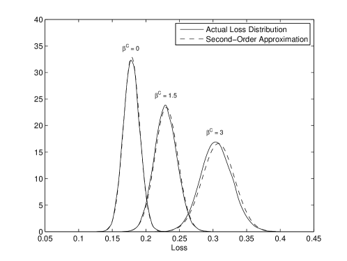
Appendix A Performance of Numerical Schemes

This appendix provides additional numerical results on the performance of the numerical schemes described in Sections 5.3.1 and 5.3.2.

In Figure 6, we compare the standard error of Schemes 1 and 2 when estimating the expectation of f(LTN)=(LTNS)+𝑓superscriptsubscript𝐿𝑇𝑁superscriptsuperscriptsubscript𝐿𝑇𝑁𝑆f(L_{T}^{N})=(L_{T}^{N}-S)^{+} (i.e., a call option on the portfolio loss). Parameters are a time step of 0.0050.0050.005, strike S=0.12𝑆0.12S=0.12, and K=6𝐾6K=6 as the truncation level. Scheme 1 is performed using an optimal choice of J𝐽J and M𝑀M given by (14). For small βSsuperscript𝛽𝑆\beta^{S}, Scheme 2 outperforms Scheme 1 since the conditionally Gaussian noise dominates. For large βSsuperscript𝛽𝑆\beta^{S}, the process X𝑋X dominates the dynamics and the semi-analytic calculation reduces the standard deviation an insufficient amount to justify the additional computational time.

Refer to caption
Figure 6. Comparison of standard error for Scheme 111 and Scheme 222, respectively described in Sections 5.3.1 and 5.3.2. Parameter case is T=0.5,N=500,σ=0.9,α=4,λ0=λ¯=0.2,formulae-sequence𝑇0.5formulae-sequence𝑁500formulae-sequence𝜎0.9formulae-sequence𝛼4subscript𝜆0¯𝜆0.2T=0.5,N=500,\sigma=0.9,\alpha=4,\lambda_{0}=\bar{\lambda}=0.2, and βC=1superscript𝛽𝐶1\beta^{C}=1. The systematic risk X𝑋X is an OU process with mean 111, reversion speed 222, volatility 111, and initial value 111.

We also compare the standard error of the second-order approximation (calculated using Scheme 1) and direct simulation of the original finite system (1) in Figure 7.

Refer to caption
Figure 7. Comparison of standard error for direct simulation of the finite system and the second-order approximation. Parameter case is T=0.5,σ=0.9,α=4,λ0=λ¯=0.2,βC=1,formulae-sequenceformulae-sequence𝑇0.5formulae-sequence𝜎0.9formulae-sequence𝛼4subscript𝜆0¯𝜆0.2superscript𝛽𝐶1T=0.5,\sigma=0.9,\alpha=4,\lambda_{0}=\bar{\lambda}=0.2,\beta^{C}=1, and βS=1superscript𝛽𝑆1\beta^{S}=1. The systematic risk X𝑋X is an OU process with mean 111, reversion speed 222, volatility 111, and and initial value 111.

We use a truncation level of K=6𝐾6K=6 and a time step of 0.0050.0050.005 for both asymptotic and finite systems. We report exact values in the following table for a total computational time of 505050 seconds. For N=1,000𝑁1000N=1,000 and N=2,500𝑁2500N=2,500, the second-order approximation has a standard error roughly one order of magnitude smaller than the finite system simulation. This means that for the standard errors to be equal, one must invest roughly two orders of magnitude more computational resources into the finite system simulation.

Finite System Second-order Approximation
Standard Error (N=1,000𝑁1000N=1,000) 1.00 ×10³absentsuperscript103\times 10^{-3} 1.39 ×10⁴absentsuperscript104\times 10^{-4}
Standard Error (N=2,500𝑁2500N=2,500) 1.40 ×10³absentsuperscript103\times 10^{-3} 1.24 ×10⁴absentsuperscript104\times 10^{-4}

References

  • [1] \harvarditemAdams1978Adams1978 Adams, Robert A. \harvardyearleft1978\harvardyearright, Sobolev spaces, Academic Press, New York.
  • [2] \harvarditem[Azizpour et al.]Azizpour, Giesecke \harvardand Schwenkler2010azizpour-giesecke-schwenkler Azizpour, Shahriar, Kay Giesecke \harvardand Gustavo Schwenkler \harvardyearleft2010\harvardyearright, Exploring the sources of default clustering. Working Paper, Stanford University.
  • [3] \harvarditemBeskos \harvardand Roberts2005Beskos Beskos, Alexander \harvardand Gareth Roberts \harvardyearleft2005\harvardyearright, ‘Exact simulation of diffusions’, Annals of Applied Probability 15(4), 2422–2444.
  • [4] \harvarditemBurkholder1973Burkholder Burkholder, Donald L. \harvardyearleft1973\harvardyearright, ‘Distribution function inequalities for martingales’, Annals of Probability 1, 19–42.
  • [5] \harvarditem[Bush et al.]Bush, Hambly, Haworth, Jin \harvardand Reisinger2011hambly Bush, Nick, Ben Hambly, Helen Haworth, Lei Jin \harvardand Christoph Reisinger \harvardyearleft2011\harvardyearright, ‘Stochastic evolution equations in portfolio credit modelling’, SIAM Journal on Financial Mathematics 2, 627–664.
  • [6] \harvarditemChen \harvardand Huang2012chen Chen, Nan \harvardand Zhengyu Huang \harvardyearleft2012\harvardyearright, Localization and exact simulation of Brownian motion driven stochastic differential equations. Mathematics of Operations Research, forthcoming.
  • [7] \harvarditem[Cvitanić et al.]Cvitanić, Ma \harvardand Zhang2012CMZ Cvitanić, Jakša, Jin Ma \harvardand Jianfeng Zhang \harvardyearleft2012\harvardyearright, ‘The law of large numbers for self-exciting correlated defaults’, Stochastic Processes and Their Applications 122(8), 2781–2810.
  • [8] \harvarditemDai Pra \harvardand Tolotti2009daipra-tolotti Dai Pra, Paolo \harvardand Marco Tolotti \harvardyearleft2009\harvardyearright, ‘Heterogeneous credit portfolios and the dynamics of the aggregate losses’, Stochastic Processes and their Applications 119, 2913–2944.
  • [9] \harvarditem[Dai Pra et al.]Dai Pra, Runggaldier, Sartori \harvardand Tolotti2009daipra-etal Dai Pra, Paolo, Wolfgang Runggaldier, Elena Sartori \harvardand Marco Tolotti \harvardyearleft2009\harvardyearright, ‘Large portfolio losses: A dynamic contagion model’, The Annals of Applied Probability 19, 347–394.
  • [10] \harvarditem[Das et al.]Das, Duffie, Kapadia \harvardand Saita2007ddk Das, Sanjiv, Darrell Duffie, Nikunj Kapadia \harvardand Leandro Saita \harvardyearleft2007\harvardyearright, ‘Common failings: How corporate defaults are correlated’, Journal of Finance 62, 93–117.
  • [11] \harvarditem[Del Barrio et al.]Del Barrio, Deheuvels \harvardand Geer2007BarrioDeheuvelsGeer2007 Del Barrio, Eustasio, Paul Deheuvels \harvardand Sara Van De Geer \harvardyearleft2007\harvardyearright, Lectures on Empirical Processes: Theory and Statistical Applications, European Mathematical Society Publishing House, Zurich.
  • [12] \harvarditemEthier \harvardand Kurtz1986MR88a:60130 Ethier, Stewart N. \harvardand Thomas G. Kurtz \harvardyearleft1986\harvardyearright, Markov Processes: Characterization and Convergence, John Wiley & Sons Inc., New York.
  • [13] \harvarditemFernandez \harvardand Mélèard1997FernandezMeleard Fernandez, Begoña \harvardand Sylvie Mélèard \harvardyearleft1997\harvardyearright, ‘A hilbertian approach for fluctuations on the mckean-vlasov model’, Stochastic Processes and their Applications 71, 33–53.
  • [14] \harvarditemFouque \harvardand Ichiba2012fouque-ichiba Fouque, Jean-Pierre \harvardand Tomoyuki Ichiba \harvardyearleft2012\harvardyearright, ‘Stability in a model of interbank lending’, SIAM Journal on Financial Mathematics . to appear.
  • [15] \harvarditem[Garnier et al.]Garnier, Papanicolaou \harvardand Yang2012PapanicolaouSystemicRisk Garnier, Josselin, George Papanicolaou \harvardand Tzu-Wei Yang \harvardyearleft2012\harvardyearright, ‘Large deviations for a mean field model of systemic risk’, SIAM Journal on Financial Mathematics 4, 151–184.
  • [16] \harvarditemGel’fand \harvardand Vilenkin1964GelfandVilenkin1964 Gel’fand, I.M. \harvardand N.Ya Vilenkin \harvardyearleft1964\harvardyearright, Generalized Functions, Vol. 4: Applications of Harmonic Analysis, Academic Press, New York-London.
  • [17] \harvarditemGiesecke \harvardand Smelov2012smelov Giesecke, Kay \harvardand Dmitry Smelov \harvardyearleft2012\harvardyearright, Exact sampling of jump-diffusions. Operations Research, forthcoming.
  • [18] \harvarditemGiesecke \harvardand Schwenkler2011giesecke-schwenkler Giesecke, Kay \harvardand Gustavo Schwenkler \harvardyearleft2011\harvardyearright, Filtered likelihood for point processes. Working Paper, Stanford University.
  • [19] \harvarditem[Giesecke et al.]Giesecke, Spiliopoulos \harvardand Sowers2013GieseckeSpiliopoulosSowers2011 Giesecke, Kay, Konstantinos Spiliopoulos \harvardand Richard Sowers \harvardyearleft2013\harvardyearright, ‘Default clustering in large portfolios: Typical events’, The Annals of Applied Probability 23(1), 348–385.
  • [20] \harvarditem[Giesecke et al.]Giesecke, Spiliopoulos, Sowers \harvardand Sirignano2012GieseckeSpiliopoulosSowersSirigano2012 Giesecke, Kay, Konstantinos Spiliopoulos, Richard Sowers \harvardand Justin A. Sirignano \harvardyearleft2012\harvardyearright, Large portfolio asymptotics for loss from default. Mathematical Finance, forthcoming.
  • [21] \harvarditemGiesecke \harvardand Weber2006giesecke-weber Giesecke, Kay \harvardand Stefan Weber \harvardyearleft2006\harvardyearright, ‘Credit contagion and aggregate losses’, Journal of Economic Dynamics and Control 30, 741–767.
  • [22] \harvarditemGyöngy \harvardand Krylov1990GyongiKrylov1992 Gyöngy, Imre \harvardand Nikolai Krylov \harvardyearleft1990\harvardyearright, ‘Stochastic partial differential equations with unbounded coefficients and applications, I’, Stochastics and Stochastics Reports 32, 53–91.
  • [23] \harvarditemJoffe \harvardand Métivier1986JoffeMetivier1986 Joffe, A. \harvardand M. Métivier \harvardyearleft1986\harvardyearright, ‘Weak convergence of sequences of semimartingales with applications to multitype branching processes’, Advances in Applied Probability 18, 20–65.
  • [24] \harvarditemKim2009Kim2009 Kim, Kyeong-Hun \harvardyearleft2009\harvardyearright, ‘Sobolev space theory of SPDEs with continuous or measurable leading coefficients’, Stochastic Processes and their Applications 119(1), 16–44.
  • [25] \harvarditemKrylov \harvardand Lototsky1998KryLot1998 Krylov, Nicolai \harvardand Sergey Lototsky \harvardyearleft1998\harvardyearright, ‘A Sobolev space theory of SPDEs with constant coefficients on a half line’, SIAM Journal of Mathematical Analysis 30(2), 298–325.
  • [26] \harvarditemKurtz \harvardand Xiong2004KurtzXiong Kurtz, Thomas G. \harvardand Jie Xiong \harvardyearleft2004\harvardyearright, ‘A stochastic evolution equation arising from the fluctuations of a class of interacting particle systems’, Communications in Mathematical Sciences 2(3), 325–358.
  • [27] \harvarditemKurtz \harvardand Protter1996KurtzProtter Kurtz, Thomas G. \harvardand Philip Protter \harvardyearleft1996\harvardyearright, Weak convergence of stochastic integrals and differential equations, II. Infinite-dimensional case, in ‘Probabilistic models for nonlinear partial differential equations, Lecture Notes in Mathematics’, Springer-Verlag, pp. 197–285.
  • [28] \harvarditemLototsky2001Lot2001 Lototsky, Sergey \harvardyearleft2001\harvardyearright, ‘Linear stochastic parabolic equations degenerating on the boundary of a domain’, Electronic Journal of Probability 6(24), 1–14.
  • [29] \harvarditemMétivier1985Metivier1985 Métivier, M. \harvardyearleft1985\harvardyearright, Weak convergence of measure valued processes using sobolev embedding techniques, in ‘Proceedings Stochastic Partial Differential Equations, Lecture Notes in Mathematics, Vol. 1236’, Springer-Verlag, pp. 172–183.
  • [30] \harvarditemPurtukhia1984Purtukhia1984 Purtukhia, O.G. \harvardyearleft1984\harvardyearright, On the equations of filtering of multi-dimensional diffusion processes (unbounded coefficients). Thesis, Moscow, Lomonosov University 1984 (in Russian).
  • [31] \harvarditemRoyden1988MR90g:00004 Royden, Halsey \harvardyearleft1988\harvardyearright, Real analysis, third edn, Macmillan Publishing Company, New York.
  • [32]