Molecular Cloud Evolution V. Cloud Destruction by Stellar Feedback

Abstract

We present a numerical study of the evolution of molecular clouds, from their formation by converging flows in the warm ISM, to their destruction by the ionizing feedback of the massive stars they form. We improve with respect to our previous simulations by including a different stellar-particle formation algorithm, which allows them to have masses corresponding to single stars rather than to small clusters, and with a mass distribution following a near-Salpeter stellar IMF. We also employ a simplified radiative-transfer algorithm that allows the stellar particles to feed back on the medium at a rate that depends on their mass and the local density. Our results are as follows: a) Contrary to the results from our previous study, where all stellar particles injected energy at a rate corresponding to a star of $\sim 10~{}M_{\odot}$, the dense gas is now completely evacuated from 10-pc regions around the stars within 10–20 Myr, suggesting that this feat is accomplished essentially by the most massive stars. b) At the scale of the whole numerical simulations, the dense gas mass is reduced by up to an order of magnitude, although star formation (SF) never shuts off completely, indicating that the feedback terminates SF locally, but new SF events continue to occur elesewhere in the clouds. c) The SF efficiency (SFE) is maintained globally at the $\sim 10\%$ level, although locally, the cloud with largest degree of focusing of its accretion flow reaches SFE $\sim 30\%$. d) The virial parameter of the clouds approaches unity before the stellar feedback begins to dominate the dynamics, becoming much larger once feedback dominates, suggesting that clouds become unbound as a consequence of the stellar feedback, rather than unboundness being the cause of a low SFE. e) The erosion of the filaments that feed the star-forming clumps produces chains of isolated dense blobs reminiscent of those observed in the vicinity of the dark globule B68.

1 Introduction

Understanding how star formation (SF) proceeds in our Galaxy, and other galaxies in general, is a key quest in astrophysics. In recent years, it has become clear that the evolution and distribution of SF in the Galaxy is intimately linked to the structure and evolution of the molecular clouds (MCs) where it takes place (see, e.g., the reviews by Mac Low & Klessen, 2004; Ballesteros-Paredes et al., 2007; McKee & Ostriker, 2007; Vázquez-Semadeni, 2013, and references therein).

In a series of previous papers (Vázquez-Semadeni et al., 2006, 2007, 2010, 2011), we have investigated, alongside other groups (Hennebelle & Pérault, 1999, 2000; Audit & Hennebelle, 2005; Hennebelle & Audit, 2007; Audit & Hennebelle, 2010; Hennebelle et al., 2008; Heitsch et al., 2005; Heitsch et al, 2006; Heitsch & Hartmann, 2008; Heitsch et al., 2009; Banerjee et al., 2009), the evolution of MCs and of their SF activity, from their formation by condensation of the atomic gas in the interstellar medium to their star-forming stages and, in some studies, to their destruction by stellar feedback (Vázquez-Semadeni et al., 2010). Among the above studies, those including self-gravity (Vázquez-Semadeni et al., 2007, 2010, 2011; Heitsch & Hartmann, 2008; Heitsch et al., 2009) have shown that the coherent formation of large clouds (several tens of parsecs) leads to the onset of global gravitational contraction throughout the cloud, at a stage when the cloud is still mostly composed of atomic hydrogen, with SF only starting several Myr later, when the cloud has become mostly molecular.

This result, however, is in contradiction with the largely established notion that MCs cannot be collapsing freely, since otherwise their resulting SF rates (SFRs) would be up to two orders of magnitude larger than observed (Zuckerman & Palmer, 1974). A related property is that the observed SF efficiency (SFE, the fraction of a cloud’s mass that ends up in stars) for whole giant molecular clouds (GMCs) is estimated to be of only a few percent (e.g. Myers et al., 1986; Evans et al., 2009; Federrath & Klessen, 2013). Hence, it is generally believed that MCs must be in or near equilibrium, supported against their self-gravity by supersonic turbulence, magnetic fields, or some combination thereof. Specifically, a number of SF theories have appeared in recent years in which the underlying scenario is that MCs are supported globally by turbulent pressure, while gravitational collapses occur only locally, caused by the supersonic turbulent compressions (e.g., Padoan & Nordlund, 2002, 2011; Krumholz & McKee, 2005; Hennebelle & Chabrier, 2011, see also the discussion by Federrath & Klessen 2012).

Of course, an alternative explanation has been known for over four decades (e.g., Field, 1970; Whitworth, 1979; Elmegreen, 1983; Cox, 1983; Franco, Shore & Tenorio-Tagle, 1994) for the low observed SFE of GMCs, namely that stellar feedback, mainly from the ionizing radiation from massive stars, may disrupt the clouds before they have converted much of their mass into stars. In this scenario, there is no need to support the clouds against their self-gravity. Also, this scenario becomes even more feasible in view of the recent result, from numerical simulations of cloud formation and evolution, that the collapsing clouds undergo hierarchical gravitational fragmentation (Vázquez-Semadeni et al., 2009). That is, the turbulent density fluctuations, having larger mean densities than that of the whole parent GMC, have shorter free-fall times and smaller Jeans masses, and therefore the densest clumps begin to form stars earlier than the rest of the cloud, and before the global collapse of the cloud terminates.

In Vázquez-Semadeni et al. (2010, hereafter Paper I), we carried out a first attempt to numerically capture this phenomenology, by performing simulations of cloud formation and evolution in the presence of ionization heating from massive stars, which is considered to be the main feedback mechanism affecting GMCs of masses up to $\sim 10^{5}~{}M_{\odot}$ (Matzner, 2002; Krumholz & Matzner, 2009; Dale et al., 2012). In Paper I, the instantaneous, time-dependent SFE was defined as

$$\hbox{SFE}(t)=\frac{{M_{*}}(t)}{M_{\rm dense}(t)+{M_{*}}(t)},$$ (1)

where $M_{\rm dense}$ is the mass in dense gas ($n>100{\rm~{}cm}^{-3}$) and ${M_{*}}$ is the total mass in stars. It was found in that paper that the prescription for ionization-heating feedback used there was able to maintain the SFE at the few-percent level throughout the evolution of the cloud, while control simulations not including it reached SFEs roughly an order of magnitude larger. Also, an analytical model representing this scenario was recently presented by Zamora-Avilés et al. (2012), and shown to correctly describe several evolutionary properties of GMCs and their SF activity.

However, one shortcoming of the feedback prescription used in Paper I was that it assumed that the stars responsible for the feedback all injected energy into the medium at a rate roughly corresponding to that of a $\sim 10~{}M_{\odot}$ star. This implied that the stellar feedback was possibly overestimated for clouds forming low-mass stars, and underestimated for clouds forming high-mass stars. In particular, Paper I found that the GMC-like clouds could not be destroyed by the feedback. Instead, Dale et al. (2012), for example, have been able to disrupt clouds up to $10^{6}~{}M_{\odot}$ by means of ionization feedback. In Paper I, the SFE was kept low because the conversion of dense gas into stars was locally inhibited by the feedback, but not because the clouds at large were destroyed. Only the local clumps were destroyed.

In the present paper, we improve on the numerical prescription used in Paper I in two ways. First, we use a probabilistic SF prescription instead of a fully deterministic one. As it turns out, this probabilistic prescription allows us to produce a mass spectrum for stellar particles, which can be tuned to resemble the Salpeter initial mass function (IMF). Second, once armed with a realistic stellar mass spectrum, we incorporate a mass-dependent ionization heating prescription for the feedback from the stellar particles produced in the simulations, applying a simplified description of radiative transfer, neglected in Paper I. We expect that, with this prescription, we can obtain a more realistic description of the effect of ionization feedback on MCs of various masses.

The plan of the paper is as follows. In Sec. 2, we describe the numerical model, focusing in particular on the heating and cooling functions employed (Sec. 2.2), the stellar-particle formation prescription (Sec. 2.3), the feedback prescription (Sec. 2.4), and the refinement criterion used (Sec. 2.1). We next describe the details and parameters of the simulations in Sec. 3, and then present our results in Sec. 4. In Sec. 5 we compare our results with those of Paper I and discuss some of their implications. Finally, in Sec. 6 we present a summary and some conclusions.

2 The Numerical Model

The numerical simulations used in this work were performed using the adaptive mesh refinement (AMR) + N-body Adaptive Refinement Tree code ART (Kravtsov et al., 1997, 2003). In the following sections we describe the adaptations we have performed to it for application to our problem of interest.

2.1 Refinement

The numerical box is initially covered by a grid of $128^{3}$ (zeroth level) cells. The mesh is subsequently refined as the matter distribution evolves. The maximum allowed refinement level was set to five, so that high-density regions have an effective resolution of $4096^{3}$ cells, with a minimum cell size of 0.0625 pc. As in Paper I, cells are refined when the gas mass within the cell is greater than $0.32M_{\odot}$. That is, the cell size is refined by a factor of 2 when the density increases by a factor of 8, so that, while refinement is active, the grid cell size $\Delta x$ scales with density $n$ as $\Delta x\propto n^{-1/3}$. Once the maximum refinement level is reached, no further refinement is performed, and the cell’s mass can reach much larger values.

Note that this constant-cell-mass refinement criterion does not conform to the so-called Jeans criterion (Truelove et al., 1997) of resolving the Jeans length with at least 4 grid cells. Truelove et al. (1997) cautioned that failure to do this might result in spurious, numerical fragmentation. However, we do not consider this a cause for concern since, as will be described in Sec. 2.3, our star formation prescription allows us to choose the stellar-particle mass distribution, and tune it to a Salpeter (1955) value.

2.2 Heating and cooling

The main additional physical processes implemented in our simulations, and relevant to the physical problem studied here are a) the cooling and heating of the gas; b) its conversion into stars; c) the stellar feedback via ionization-like heating, and d) the self-gravity from gas and stars.

We use heating ($\Gamma$) and cooling ($\Lambda$) functions of the form

$$\Gamma = 2.0\times 10^{-26}\hbox{ erg s}^{-1}$$ (2)

$$\frac{\Lambda(T)}{\Gamma} = 10^{7}\exp\left(\frac{-1.184\times 10^{5}}{T+1000}\right)$$ (3)

$$+ 1.4\times 10^{-2}\sqrt{T}\exp\left(\frac{-92}{T}\right)~{}{\rm cm}^{3}.$$

These functions are fits to the various heating and cooling processes considered by Koyama & Inutsuka (2000), as given by equation (4) of Koyama & Inutsuka (2002). As noted in Vázquez-Semadeni et al. (2007), eq. (4) in Koyama & Inutsuka (2002) contains two typographical errors. The form used here incorporates the necesary corrections, kindly provided by H. Koyama (2007, private communication). With these heating and cooling functions, the gas is thermally unstable in the density range $1\la n\la 10\ {\rm~{}cm}^{-3}$.

2.3 Star formation prescription: a probabilistic approach

In our simulations, SF is modeled as taking place in the densest regions, defined by $n>n_{\rm SF}$, where $n$ is the gas density, and $n_{\rm SF}$ is a density threshold. If a grid cell meets this density criterion, then a stellar particle (SP) of mass $m_{*}$ may be placed in the cell, with probability $P$, every timestep of the coarsest grid. If the SP is created, it acquires half of the mass of its parent cell, and this mass is removed from the cell. Thereafter, the particle is treated as non-collisional and follows N-body dynamics. No other criteria are imposed. We set $n_{\rm SF}=9.2\times 10^{4}{\rm~{}cm}^{-3}$, which corresponds to a cell mass of $0.78\ M_{\odot}$ at the highest refinement level. This fixes the minimum value for SP masses at $0.39\ M_{\odot}$. Note that, as in Paper I, our SPs differ from the commonly-used sink particles (Bate et al., 1995; Federrath et al., 2010), mainly in that our SPs are not allowed to accrete after they form. Thus, we refrain from calling them as “sinks”, and use the nomenclature “stellar particles” instead. However, as we describe below, our probabilistic approach to SP formation allows us to obtain a realistic mass distribution (IMF) for them.

A few items are worth noting about our SF prescription. First, note that, once the maximum refinement level is reached, no further refinement is applied to a cell (cf. Sec. 2.1) even if its density keeps increasing. Moreover, since the creation of an SP is a probabilistic event, the density of a cell where a gravitational collapse is going on continues to increase until an SP forms in the cell. Some authors have advocated the prescription that, once the maximum refinement level has been reached, a sink particle is created at the cell density that would correspond to the next refinement level (e.g., Federrath et al., 2010) in order to always fulfill the Jeans criterion and thus completely avoid spurious fragmentation (Truelove et al., 1997) until the sink particles are formed. However, we forgo of this recommendation since, as will be seen in what follows, our prescription allows us to impose the desired IMF of the SPs, and thus artificial fragmentation is not a concern.

The prescription we use implies that the longer it takes to form an SP in a collapsing cell, the more massive the SP will be, because the cell’s density will be higher. The probability of not having formed an SP after $n_{\rm steps}$ time steps is ${\cal P}_{\rm no}=(1-P)^{n_{\rm steps}}$, while the probability of having formed it is ${\cal P}_{\rm yes}=1-(1-P)^{n_{\rm steps}}$. These probabilities are shown in Fig. 1 for $P=0.001$.

Figure 1: Probability of having (solid line) and not having formed (dashed line) a stellar particle (SP) in a cell that meets the density criterion $n>n_{\rm SF}$ after a certain number of coarse-grid time steps for $P=0.001$.

Serendipitously, we have found that the resulting mass distribution of the SPs is a power law, with an exponent that depends on the value of $P$. Thus, $P$ is a control parameter that allows us to generate a stellar mass spectrum with the desired slope. In Figure 2 we show the evolution of the stellar mass spectrum in simulation LAF1_5l (cf. Sec. 3) with $P=0.003$. The slope of the function changes from $-1.21$ at $t=25.6$ Myr to $-1.34$ at the end of the evolution, thus hovering close to the Salpeter value of $-1.35$. The most massive SP formed in this simulation has $m_{*}=61\ M_{\odot}$, while the least massive ones have masses $m_{*}\sim 0.5~{}M_{\odot}$. Note that we have no turnover of the IMF at small masses, but this is inconsequential for our purposes, since we are only interested in the feedback exerted by the stars on their parent cloud, and the low-mass stars exert no significant feedback at the GMC scale (see, e.g., the review by Vázquez-Semadeni, 2011, and references therein)

Figure 2: Evolution of the spectrum of stellar masses for simulation LAF1_5l. The spectrum at any epoch can be well fitted by a power law. In the lower right panel, with a line, we also show this fit and the value of its slope.

We note that, because now the SPs form in cells whose density is typically much larger than the threshold value $n_{\rm SF}$, in the present paper we choose $n_{\rm SF}=9.2\times 10^{4}~{}{\rm~{}cm}^{-3}$, to allow for a sufficiently large number of SPs to form. This is significantly smaller than the value used in Paper I, where SPs formed always at a density very similar to $n_{\rm SF}$. Moreover, we stress that, contrary to the situation in our previous papers, our SPs now have masses corresponding to individual stars rather than to small clusters, and so, in what follows, we shall indistinctly refer to them simply as “stars”.

An important concern is whether our probabilistic prescription introduces a significant delay for the formation of massive stars, in comparison to the relevant timescales in the simulations. To check for this, we note that, according to a probabilistic sampling of the IMF, a 10-$M_{\odot}$ star should appear after $\approx 106.4~{}M_{\odot}$ of gas have been converted to stars, so we can check whether the formation of such a star is significantly delayed with respect to the time when this much mass has been converted into stars in the simulations. We find that, in run SAF1 (see Sec. 3), SF starts at $t=18.39$ Myr, while $106.4M_{\odot}$ worth of stars are reached at $t=21.1$ Myr, and a 10-$M_{\odot}$ star appears at t = 21.3, so the time taken by the simulation to form such a massive star coincides within less than 10% with the time needed for such a star to appear according to a statistical sampling of the IMF. In run LAF1, these times are, respectively, 18.74, 20.94, and 20.03 Myr, and so, in fact, a massive star forms slightly earlier than the time at which $106.4M_{\odot}$ worth of stars are present. So, we conclude that there is no significant delay introduced by our prescription.

2.4 Feedback prescription

Another important difference of our new feedback prescription, compared to that in Paper I, is in the way we implement the ionization feedback by massive stars. In Paper I, SPs injected thermal energy only to the cell where they were located (hereafter, the “stellar cell”), at a rate high enough to produce a realistic HII region. Instead, here we now model the birth and evolution of HII regions by assigning a temperature of $10^{4}$ K to all cells whose distance $d$ to the SP satisfies the condition

$$d<R_{\rm s}\equiv\left(\frac{3}{4\pi}\frac{S_{*}}{\alpha n_{\rm LOS}^{2}}\right)^{1/3},$$ (4)

where $R_{\rm s}$ is the Strömgren (1939) radius, $S_{*}$ is the flux of ionizing photons produced by the star, $\alpha=3.0\times 10^{-13}$ cm³ s^-1 is the recombination coefficient, and $n_{\rm LOS}$ is a characteristic particle number density along the line of sight between the stellar cell and the test cell, which we discuss below. If it turns out that $R_{\rm s}$ is smaller than the size of the stellar cell, we simply set the temperature of this cell equal to $10^{4}$ K, and no further calculation is done. On the other hand, if $R_{\rm s}$ is larger than the stellar cell’s size, then it is necessary to determine whether $d<R_{\rm s}$ or not. In principle, this poses a radiative transfer problem since, as is well known, eq. (4) is valid only for the case when the medium between the stellar and the test cells has a uniform density. However, if the medium is not uniform, then the photoionization-recombination balance must be computed along the line joining the SP and the grid cell in question (see, e.g., Dale et al., 2007), a procedure that can be quite computationally expensive.

As a zeroth-order approximation to solve this problem, we opt for choosing a value for $n_{\rm LOS}$ that can be deemed representative of the typical density along the path from the SP to the grid cell. Specifically, we take the geometric mean of the densities at these two locations in the simulation, $n_{\rm LOS}=\sqrt{n_{\rm SP}~{}n_{\rm test}}$. This approximation for $R_{\rm s}$ is, of course, crude, and will miss, for example, shadowing effects due to intervening dense clumps between the stellar and the test cells but, for the purpose of modeling the large-scale dynamics of the MC containing these cells, we consider it is sufficient. We jokingly refer to this scheme as a “poor man’s radiative transfer” (PMRT) scheme.

For the ionizing flux $S_{*}$, which depends on the SP’s mass, we use the tabulated data provided by Díaz-Miller et al. (1998). Note that only SPs with a mass greater than $1.9~{}M_{\odot}$ inject any significant ionizing feedback into the ISM, implying that only the massive SPs influence the dynamics of the molecular clouds. Finally, note that we turn off the cooling for the cells whose temperature is set to $10^{4}$ K. Otherwise, very dense cells would radiate away their thermal energy very quickly. Their temperature is held at $10^{4}$ K for a time $t_{\rm s}$, which we assume depends on the star’s mass $m_{*}$ as

$$t_{\rm s}=\left\{\begin{array}[]{ll}\mbox{2 Myr}&\mbox{if $m_{*}\leq 8M_{\odot}$};\\ 222~{}\mbox{Myr}~{}\left(\frac{m_{*}}{M_{\odot}}\right)^{-0.95}&\mbox{if $m_{*}>8M_{\odot}$}.\end{array}\right.$$ (5)

For stars more massive than $8M_{\odot}$, this time is a fit to the stellar lifetimes by Bressan etal. (1993), while for stars with masses lower than that, it represents the fact that the duration of the stellar-wind phase is $\sim 2$ Myr, roughly independently of mass. This also means that we are representing the effect of the winds and outflows of low mass stars by an ionization prescription. While this is clearly only an approximation, we do not expect it to have much impact on our calculations, since the main source of feedback energy at the level of GMCs is the ionization feedback from massive stars (Matzner, 2002).

Our prescription for the ionization feedback for massive stars was tested by running simulations of a box of 32 pc on a side, without self-gravity, filled with gas at uniform temperature and density, of 42 K and $100{\rm~{}cm}^{-3}$, respectively. These simulations used a resolution of $256^{3}$ cells, with the adaptive refinement switched off. A massive SP ($m_{*}=27~{}M_{\odot}$) was placed in the center of the box, and the system was allowed to evolve freely. Figure 3 shows the expansion of the resulting HII region, which is comprised of those cells with temperatures greater than a few thousand degrees. Also shown in this figure is the well known analytical solution (Spitzer, 1978),

$$R_{s}(t)=R_{i}\left(1+\frac{7}{4}\frac{c_{s}t}{R_{i}}\right)^{4/7},$$ (6)

where $R_{i}$ is the initial Strömgren radius and $c_{s}$ is the sound speed. The numerical solution is seen to agree with the analytic one to within $\sim 30$%, an accuracy we consider sufficient, given our interest only in the large-scale evolution of the clouds.

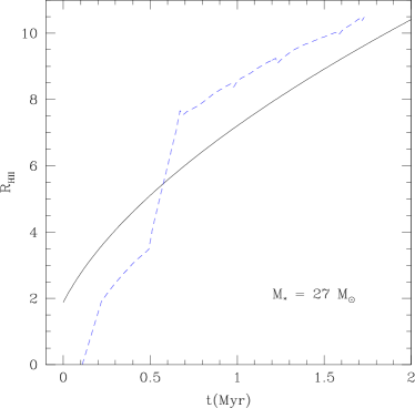
Figure 3: Evolution of the HII region produced by a $27$-$M_{\odot}$ star in a box of 32 pc per side. The black solid line represents the analytic solution given by eq. (6), while the blue dashed line is the radius of the HII region in the simulation. Temperatures of target cells located inside the Strömgren sphere, centered on the SP, are set to $10^{4}$ K. The cooling is switched off in these cells during the lifetime of the star.

3 The simulations

Our simulations use the same initial setup as the runs in Paper I, which represents the evolution of a region of 256 pc per side, initially filled with warm gas at a uniform density of $n_{0}=1{\rm~{}cm}^{-3}$ and a temperature $T_{0}=5000$ K, implying an adiabatic sound speed $c_{\rm s}=7.4{\rm~{}km~{}s}^{-1}$ (assuming a mean particle mass $\mu=1.27$). The full numerical box thus contains $5.25\times 10^{5}M_{\odot}$. In this medium, we make two streams collide with a speed $v_{\rm inf}=5.9{\rm~{}km~{}s}^{-1}$ each (corresponding to a Mach number of 0.8 with respect to the unperturbed medium) along the $x$-direction (see Figure 1 of Vázquez-Semadeni et al., 2007). The streams have a radius of 64 pc and a length of 112 pc each, so that the total mass in the two inflows is $9.0\times 10^{4}M_{\odot}$. Note that the streams are completely contained within the box, so that the compression they produce is a single event. There is no continuous flow through the boundaries, as we use periodic boundary conditions.

Table 1: Parameters of the Simulations

Run	$v_{\rm rms}$	Feedback
name	[km s-1]
SAF1	0.1	New prescription, full IMF
LAF1	1.7	New prescription, full IMF
LAF0	1.7	Off
LAFold	1.7	Old prescription from Paper I
LAF8	1.7	New prescription, max stellar mass $=8~{}M_{\odot}$
LAF20	1.7	New prescription, max stellar mass $=20~{}M_{\odot}$

On top of the inflow velocity we superpose a field of initial low-amplitude turbulent velocity fluctuations, in order to trigger the instabilities in the compressed layer that will cause it to fragment and become turbulent (Heitsch et al., 2005; Vázquez-Semadeni et al., 2006). As in Paper I, we create this initial velocity fluctuation field with a new version of the spectral code used in Vázquez-Semadeni et al. (1995) and Passot et al. (1995), modified to run in parallel in shared-memory architectures. The simulations are evolved for about 40 Myr.

The collision nonlinearly triggers a transition to the cold phase, forming a turbulent, cold, dense cloud (Hennebelle & Pérault, 1999; Audit & Hennebelle, 2005; Heitsch et al., 2005; Heitsch et al, 2006; Vázquez-Semadeni et al., 2006), consisting of a complex network of sheets, filaments, and clumps of cold gas embedded in a warm diffuse substrate (Audit & Hennebelle, 2005; Hennebelle & Inutsuka, 2006; Hennebelle & Audit, 2007). The complex as a whole quickly engages in gravitational collapse (Vázquez-Semadeni et al., 2007). Moreover, the local density fluctuations become unstable and collapse in a shorter time than the global time because they are embedded in a contracting medium and thus have shorter collapse times (Toalá et al., 2013). Eventually, they proceed to forming stars, which then heat their environment, forming expanding “HII regions” that tend to disperse the clouds.

Although our results are based essentially on two simulations, a few more runs were performed with a twofold purpose: to compare the old prescription for feedback to the new one, and to assert the importance of the most massive SPs in the disruption of the clouds. All simulations but one were run using the “large-amplitude” (LA) initial velocity fluctuations ($v_{\rm rms}\sim 1.7{\rm~{}km~{}s}^{-1}$) as opposed to the “small-amplitude” (SA) case ($v_{\rm rms}\sim 0.1{\rm~{}km~{}s}^{-1}$) (see Paper I). Clearly, more fragmentation and more complex cloud structures are expected in the LA runs, thus causing them to produce somewhat smaller clouds that resemble low- or intermediate-mass star-forming clouds. On the other hand, the SA run allows us to consider a case of very high coherence and uniformity, which tends to form a high-mass star-forming region (Vázquez-Semadeni et al., 2009), and furthermore resembles the conditions we used in previous papers (Vázquez-Semadeni et al., 2007, 2011).

The nomenclature for the runs introduced in Table 1 continues to use the acronyms LAF or SAF used in Paper I, where F stands for feedback. A number 1 or 0 after the letter F means feedback is on or off, respectively. The test simulations are denoted with “old”, 8 or 20 after the word LAF.

4 Results

4.1 Evolution of the simulations

The simulations performed here behave very similarly to previous simulations with similar setups, except for the ultimate fate of the individual clouds. In particular, our SAF1 run is very similar to run L256$\Delta v$0.17 in Vázquez-Semadeni et al. (2007), the run presented by Banerjee et al. (2009), and the SAF0 and SAF1 runs in Paper I. The main feature of these runs is that, because the initial velocity fluctuations are very mild, the flow collision creates a large, coherent pancake-like structure of cold, dense gas, which soon begins to undergo global gravitational collapse. However, a recent study, in which the parameters of the flow collision are varied (Rosas-Guevara et al., 2010), has shown that the coherence of the collapse may be lost in the presence of stronger initial fluctuations. In such cases, smaller clouds appeared to be less strongly gravitationally bound, with the effect of decreasing the SFE. This behavior was also observed in the LA simulations of Paper I, and also occurs in the LAF1 run of the present paper. In this case, the cloud formed by the initial flow is much more irregular in shape, and much more fragmented and scattered over the simulation volume. As a result, SF also occurs in a much more scattered manner, and the SFEs are in general smaller in the LA runs than in their SA counterparts. Figure 4 shows an image, in projection, of the gas density field of a region of run LAF1 that encompases the clouds we discuss in the remainder of the paper: Cloud 1 (upper left corner), Cloud 2 (right off-center), and an uncharted third cloud (left off-center) in run LAF1 at $t\approx 26.3$ Myr. In the figure, stellar particles are shown as bluish dots.

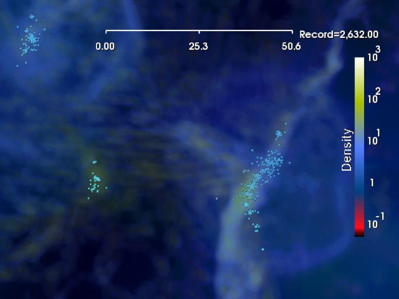
Figure 4: View in projection of the central region of run LAF1 at $t\approx 26.3$ Myr. The horizontal ruler shows a scale of 50.6 pc and we have indicated with bluish dots the stellar particles. Three star-forming clouds are seen, one at the upper left corner (Cloud 1), one to the right of the image center (Cloud 2), and uncharted, low-mass cloud at the left of the center. Shells expanding away from Clouds 1 and 2 can be seen at this time.

However, in general a common pattern is followed by all simulations: the transonic converging flows in the diffuse gas induce a phase transition to the cold phase of the atomic gas. The newly formed dense gas is highly prone to gravitational instability. This can be seen as follows. The thermal pressure at our initial conditions is 5000 K${\rm~{}cm}^{-3}$. From Fig. 2 of Vázquez-Semadeni et al. (2007), it can be seen that the thermal balance conditions of the cold medium at that pressure are $n\sim 130{\rm~{}cm}^{-3}$, $T\sim 40$ K. At these values, the Jeans length and mass are $\sim 7$ pc and $\sim 640M_{\odot}$, respectively. These sizes and masses are easily achievable by a large fraction of the cold gas structures, which can then proceed to gravitational collapse and form stars. Moreover, the ensemble of these clumps may also be gravitationally unstable as a whole, the likelihood of this being larger for greater coherence of the large-scale pattern.

Regions of active star formation form in SAF1 and LAFs runs by the gravitational merging of pre-existing smaller-scale clumps, which, altogether, form a larger-scale GMC.

Figure 5: Evolution of the mass in dense gas (top left panel), the star formation rate (SFR; dashed line) and efficiency (SFE; solid line) (top right panel), the mass in SPs (bottom left panel), and the mass in stars plus dense gas (bottom right panel) in the whole box in run SAF1. As a result of the destruction of the dense gas the mass in SPs as well as the SFE reaches a maximum before the end of the evolution.

4.2 Cloud Evolution in runs LAF1 and SAF1

The new schemes for the probabilistic star formation recipe and for the ionization feedback by massive stars were used to run the SAF1 and LAF1 simulations. Figures 5 and 6 show, for the full simulated box, the evolution of the mass in dense gas ($n>100\ {\rm~{}cm}^{-3}$), the mass in stars, the mass in both components, and the star formation rate (SFR) and efficiency (SFE), in the SAF1 and LAF1 runs, respectively. In contrast to Paper I, we now define the instantaneous SFE as

$$\hbox{SFE}(t)=\frac{{M_{*}}(t)}{M_{\rm max}(t)+{M_{*}}(t)},$$ (7)

where $M_{\rm max}$ is the maximum mass in dense gas reached between the start of the simulation and time $t$. This is because in the present simulations the clouds are eventually dispersed, and thus the SFE evaluated with the instantaneous dense gas mass approaches unity at late stages of evolution, but not because all the dense gas has been converted to stars, but rather because the remaining gas is evaporated by the stars. Our definition gives us instead an approximate measure of the net SFE, that is, the fraction of the dense gas mass ever present in a given volume and over a certain time interval that is converted into stars.

Figure 6: Evolution of the mass in dense gas (top left panel), the SFR (dashed line) and SFE (solid line; top right panel), the mass in SPs (bottom left panel), and the mass in stars plus dense gas (bottom right panel) in the whole box for run LAF1. Unlike the SA run, here the star formation does not stop abruptly, and instead a slow decline in the star formation rate is observed.

In both runs, the evolution of the mass in dense gas is similar (see the top left panels of Figs. 5 and 6): first, dense gas starts to accumulate as the evolution proceeds until it reaches a maximum, then the effect of the radiation feedback is such that it overcomes the buildup of dense gas by gravitacional accretion. Also, in both runs, SPs continue to form after the maximum in the mass in dense gas is reached, albeit at a significantly declining rate. Later in the evolution, in the LAF1 run, the mass in dense gas begins to increase again. This time the density does not reach the threshold for star formation and thus no new SPs are formed (see bottom left panels of Figs. 5 and 6).

Figure 7: Evolution of the mass in dense gas (top left panel), the SFE (top right panel), the mass in SPs (bottom left panel), and the SFR (bottom right panel) in the Central Cloud in run SAF1. Ioinization feedback is so efficient that the cloud only lives about 10 Myr. Interestingly, the stellar cluster is almost dispersed in the next 10 Myr of evolution.

In run SAF1, the largest star-forming region forms close to the center of the box, due to the coherent collapse of the entire sheet-like cloud formed by the collision. As in Paper I, we refer to this region as “the Central Cloud”. We enclose the cloud in a cylinder of radius 10 pc and length 20 pc with its center located at the instantaneous minimum of the potential within the cylindrical region, implying that the cylinder moves in time following the cloud. Figure 7 shows the evolution of the mass in dense gas, the SFE, the mass in stars, and the SFR in this cylinder. This figure is similar to Fig. 5 (or Fig. 6) except that the bottom right panel now shows the evolution of the SFR in the cylinder instead of the evolution of the gas-plus-stars mass. Unlike what happens with the whole box, where some dense gas still remains by the end of the evolution, here we witness the complete dispersal of the cloud from this region. In addition, in the lower left panel we see that the mass in SPs also decreases by the end of the evolution. Because our SPs have no winds and do not explode as supernovae, this can can only mean that the stellar cluster, formed from the dense gas mass of the cloud, is being dispersed as well (that is, its constituent stars are leaving the cylinder that initially contained the cloud).

Figure 8: Evolution of the mass in dense gas (top left panel), the SFE (top right panel), the mass in SPs (bottom left panel), and the SFR (bottom right panel) in Cloud 1 of run LAF1.

In the case of run LAF1, the clouds identified as Cloud 1 and Cloud 2 in Paper I are also used here to study the evolution of the cloud’s mass and its star formation activity. In paper I, we identified the centers of the clouds visually and enclosed them in a cylinder of the same dimensions as that used with the Central Cloud. Here, we use cylindrical regions of the same size to locate the minima of the potential and place the centers of the cylinders there at each time. As in Fig. 7, Figs. 8 and 9 also show the evolution of the mass in dense gas, the SFE, the mass in stars, and the SFR for Cloud 1 and Cloud 2, respectively. As with the Central Cloud in run SAF1, Cloud 1 is also destroyed, and no stars are left inside the cylinder where the cloud initially was; that is, the stellar cluster associated with the cloud is dispersed, in $\sim 12$ Myr. Cloud 2 is also completely destroyed, but unlike Cloud 1, here we still can find SPs inside its corresponding cylinder, as it was the case for the Central Cloud. Figure 10 shows the evolution in the neighborhood of Cloud 2 over 15 Myr, illustrating these results.

Figure 9: Evolution of the mass in dense gas (top left panel), the SFE (top right panel), the mass in SPs (bottom left panel), and the SFR (bottom right panel) in Cloud 2 of run LAF1.

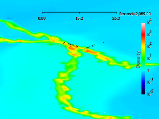
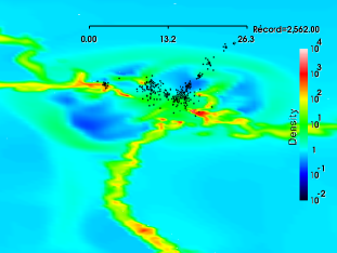
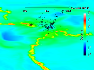
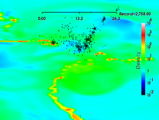
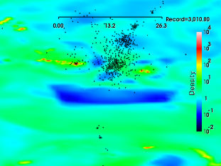
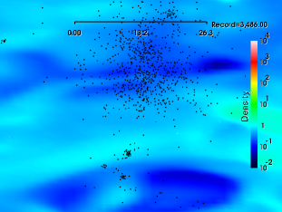
Figure 10: Cross-section images of the density field in the neighborhood of Cloud 2 in run LAF1, at times (in Myr) 20.59 (top left), 25.62 (top right), 27.02 (middle left), 27.58 (middle right), 30.1 (bottom left), and 34.86 (bottom right), showing the dispersal of the cloud. The black dots show the stellar particles (SPs). The horizontal ruler shows a scale of 26.3 pc. Note that the density field is shown on an inclined cross section through the simulation, but the SPs are shown in 3D space, so all particles in front to the density plane can be seen. Note the complete dispersal of the cloud within 15 Myr.

A final remark is that Clouds 1 and 2 evolve essentially independent from one another during the first several Myr after the onset of SF. As seen in Fig. 4, they are separated by nearly 60 pc. So, the shells expanding from them, at a speed of roughly $10{\rm~{}km~{}s}^{-1}$, will reach the other region only after some 6 Myr. Moreover, as will be discussed in Sec. 4.5, only stars more massive than $20M_{\odot}$ are really effective in destroying the clouds, and these only form several Myr after the onset of SF, when a large enough mass has been converted to stars that such massive stars are expected to form from a random sampling of the IMF. For example, in run LAF1, a 30-$M_{\odot}$ star forms at $t=23.5$ Myr; that is, $\sim 5$ Myr after the onset of SF. Thus, the effect of one star-forming region on the other is only expected to be important after $\sim 10$ Myr, at which time the local effect of these massive stars will have had plenty of time to act. Thus, we conclude that the effect of one cloud on the other is negligible compared to that of the local SF. However, the effect of one region on the other may be important when only one of the two clouds manages to form massive stars.

4.3 Evolution of the virial parameter

One important parameter of molecular clouds is the so called turbulent $\alpha$ parameter, defined as

$$\alpha\equiv 2K/|W|,$$ (8)

where $K=3\sigma_{\rm 1D}^{2}M/2$ is the (turbulent) kinetic energy, with $\sigma_{\rm 1D}$ the one-dimensional velocity turbulent dispersion and $M$ the cloud’s mass, and $W$ is the gravitational energy of the cloud, neglecting environmental contributions (see, e.g., Ballesteros-Paredes, 2006). For a spherical cloud of uniform density, $W=-3GM^{2}/5R$, and eq. (8) becomes

$$\alpha=\frac{5\sigma_{\rm 1D}^{2}R}{GM}\equiv\frac{M_{\rm vir}}{M},$$ (9)

where the identity defines the virial mass as $M_{\rm vir}\equiv 5\sigma_{\rm 1D}^{2}R/G$.

For a cloud in virial equilibrium, $\alpha=1$, and the fact that clouds are often found to have values of the virial parameter near unity (or masses close to the virial mass; e.g., Heyer et al., 2009) is generally interpreted as a signature of the clouds being in near virial equilibrium, while it is often stated that clouds strongly dominanted by self-gravity should have $\alpha\ll 1$. However, this would be true only if the turbulent motions could be clearly separated from the infalling motions that must develop in a collapsing cloud, a feat that is very difficult to accomplish in practice. Moreover, it has been recently pointed out by Ballesteros-Paredes et al. (2011) that the free-fall velocities are of the same order of magnitude as the virial turbulent motions since, after all, both types imply kinetic energies comparable to the gravitational energy.

In Fig. 11 we show the evolution of the $\alpha$ parameter for our three sample clouds from the onset of SF till the end of the simulations, using either the density-weighted velocity dispersion (which highlights the dense gas; solid lines) or the volume-weighted velocity dispersion (which tends to highlight the diffuse warm gas, since it occupies a larger fraction of the volume; dotted lines). Interestingly, we see that, for all three clouds, $\alpha$ for the dense gas is very close to unity, and in fact, continues to approach it until the time when sufficiently massive stars begin destroying the clouds, at which point it becomes much larger than unity. Conversely, for the diffuse, warm gas, $\alpha$ is significantly larger than unity at all times, although it becomes even larger when the massive stars begin to drive the motions.

Figure 11: Evolution of the alpha parameter for the three clouds for runs SAF1 and LAF1. Solid lines correspond to the density-weighted velocity dispersion, while dotted lines correspond to the volume-weighted one.

4.4 Feedback scheme comparison

In the feedback scheme of Paper I, HII regions were created by the injection of thermal energy from SPs. The energy was deposited entirely in the cell where the stars were located, and thus neighboring cells were heated exclusively by conduction, rather than by radiative heating. The value of the rate at which the energy was dumped was chosen so as to produce reasonably realistic HII regions. Additionally, the cooling in the heated cell was turned off, since otherwise most of energy would be radiated away in these initially very dense cells. Thus, it is not feasible to directly compare the results of our new simulations, with the PMRT scheme used in the present paper. However, it is important to compare the old prescription with the new one used in the present paper in a controlled manner, to assess the differences induced by the prescription, in addition to the differences induced by the presence of a stellar IMF. Therefore, we have run another LAF-type simulation, labeled LAFold, which uses the old feedback prescription from Paper I, and in which all SPs with $M_{*}>10\ M_{\odot}$ inject thermal energy at a rate equal to that used in Paper I.

Figure 12 shows the evolution of the mass in dense gas, the SFE, the stellar mass, and the mass in dense gas plus stars for runs LAF1 (black solid lines), LAF0 (red dotted lines) and LAFold (blue, short-dashed lines), together with two other runs to be discussed in the next section (see Table 1). We see that the LAFold run does not disrupt the clouds, in line with the results of Paper I.

4.5 The role of the most massive stars in the destruction of the clouds

To assert the importance of the feedback of the massive stars in the destruction of the clouds, two extra LAF models were run, labeled LAF8 and LAF20. LAF8 (magenta long-dashed lines in Fig. 12) is a run with the new feedback prescription, but with all SPs with $M_{*}>10\ M_{\odot}$ ionizing their surroundings as if they were a star of $8\ M_{\odot}$. LAF20 (cyan dot-dashed lines), moreover, is a run similar to LAF1 but in this case the feedback “saturates” at $20\ M_{\odot}$; that is, all SPs with $M_{*}<20\ M_{\odot}$ have the feedback they should according to their mass, but those SPs with $M_{*}\geq 20\ M_{\odot}$ exert a feedback as if they were a star of $20\ M_{\odot}$.

From Fig. 12 we see that, like run LAFold, run LAF8 does not destroy the clouds; the mass in dense gas in the whole simulated box (and in the individual clouds, not shown) continues to increase. Run LAF20 is an intermediate case between those runs in which clouds are not destroyed and run LAF1: in run LAF20, the mass in dense gas reaches a peak before the end of the evolution. Because the feedback in run LAF20 is not as strong as it is in run LAF1, this maximun is reached few Myr later. This experiment demostrates that stars with $M_{*}\geq 20\ M_{\odot}$ are crucial for the destruction of clouds of masses up to a few times $10^{4}~{}M_{\odot}$.

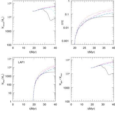
Figure 12: Evolution of the mass in dense gas (top left panel), the SFE (top right panel), the mass in SPs (bottom left panel), and the mass in stars plus dense gas (bottom right panel) in the whole numerical box of each of the five LAF runs in the whole box: run LAF1 (black solid lines); run LAF0, with no feedback (red dotted lines); run LAFold (blue short-dashed lines), with the feedback prescription from Paper I; run LAF8 (magenta long-dashed lines), with the new feedback prescription but with all SPs with $M_{*}>10\ M_{\odot}$ ionizing their surroundings as if they had a mass of $8~{}M_{\odot}$; and finally, run LAF20 (cyan dot-dashed lines), in which all SPs with $M_{*}<20\ M_{\odot}$ feed back according to their masses, but SPs with $M_{*}\geq 20\ M_{\odot}$ feed back as if they were a star of $20\ M_{\odot}$.

4.6 Formation of “dark globule” chains

An interesting feature of run LAF1 is that, while the massive stars are in the process of evaporating the dense gas, the filaments that feed the cluster-forming clump are eroded, being destroyed first where the densities are lowest. These filaments contain dense clumps, which are more resilient to the effect of the ionising heating than the rest of the filaments, and thus they remain for some time after the filamentary structures have been destroyed. This process thus leaves behind chains of dense blobs, strongly reminiscent of those observed, for example, in the vicinity of the famous dark globule B68 (e.g., Román-Zúñiga et al., 2010), as can be seen in the top-right and middle (left and right) panels of Fig. 10. In a forthcoming paper we plan to examine in detail the similarities between the surviving blobs in our simulations and the dark globules in the vicinity of Hii regions.

5 Discussion

5.1 Comparison with previous work

The effect of feedback has been studied by numerous workers, both analytically and numerically (see, e.g., the review by Vázquez-Semadeni, 2011, and references therein). In particular, the pioneering numerical simulations of Bania & Lyon (1980) included various cases of heating and cooling functions for the medium, and used radiative transfer (on a $40\times 40$ two-dimensional grid) to include the effects of photoionization from OB stars in a 180-pc square region, making them a direct precursor of this work. Even at their very limited resolution, they foresaw several outcomes of this setup, such as the formation and maintenance of a cloud population, that the clouds would be gravitationally unstable had self-gravity been included, and that the SFR would be self-consistent if 0.1–0.5 of the mass in the clouds were to go into the formation of new massive stars, thus making a prediction for the SFE. However, their required SFE for self-consistency was too high, presumably because self-gravity was not included in their simulations. This limitation also meant that the feedback stars had to be placed randomly in the simulation. Subsequent numerical works focused mostly on the effect of supernova feedback on the structuring of the ISM on kiloparsec scales (e.g., Rosen et al., 1993; Rosen & Bregman, 1995; de Avillez, 2000; Mac Low et al., 2005; Joung & Mac Low, 2006; Wood et al., 2010; Hill et al., 2012) but, in general, self-gravity has not been included in these works, and the supernova rate has been an input parameter for the simulations, rather than a self-consistent output.

Another line of study has been the simulation of feedback by stellar outflows at the clump (parsec) scale, aiming at either maintenance of the turbulence within the clumps (e.g., Li & Nakamura, 2006; Carroll et al., 2009; Cunningham et al., 2009), or at the self-regulation of star formation (e.g., Li & Nakamura, 2006; Nakamura & Li, 2007; Wang et al., 2010). The latter are closest in aim to our present study, although not in scale, as they only consider parsec-sized regions, and only outflow feedback, which corresponds to the effect of low- and intermediate-mass stars, which does not seem to be the dominant driver at the GMC scale (Matzner, 2002).

Our results in this paper are most directly comparable to those of Dale et al. (2012), who performed a parameter-space study of the disruptive effect of photoionizing radiation of molecular clouds of various masses. Thus, the basic physical processes at play in their simulations are very similar to those included in ours. Their main result is that, while clouds of masses up to $\sim 10^{5}~{}M_{\odot}$ can be readily destroyed by the ionization feedback from their newly-formed stars, clouds with $M\sim 10^{6}~{}M_{\odot}$ cannot be destroyed, as their escape velocities are larger than the sound speed in the photoionized gas. This regime is not sampled by our simulations, in which the total dense gas mass is never more massive than a few times $10^{4}~{}M_{\odot}$.

The main differences between our setup and theirs are that they use a polytropic equation of state covering only a temperature range corresponding to molecular and cold atomic gas, and that they start with a suite of initial clouds in various configurations, while we let the clouds form self-consistently out of the warm ISM. Also, they include the photoionized gas resulting from the stellar feedback, but their simulations lack the warm (neutral and ionized) substrate in which the clouds dwell, and out of which they form in our simulations. That is, in their simulations there is no possibility of the warm environment penetrating into the clouds, as proposed theoretically by Hennebelle & Inutsuka (2006), and suggested observationally by Krčo et al. (2008). Thus, our self-consistently formed clouds may be more porous, and thus less bound, than those of Dale et al. (2012). Also, our probabilistic SF prescription allows our SPs to be individual stars always and with a realistic IMF. This means that our simulations can be employed for future cluster dynamics studies. Instead, the sinks in the simulations by Dale et al. (2012) have a mass range that goes from individual stars to small clusters. Moreover, they only considered the effect of stars more massive than $20~{}M_{\odot}$, so they did not investigate the effect of stars of different masses. On the other hand, their radiative transfer algorithm is more realistic than ours, and they sample a larger parameter space. Thus, in general, it can be said that the two studies are highly complementary in nature, each one providing a different perspective of the problem: specifically, they focused on the ability of photoinizing radiation to destroy clouds of different masses, while we have focused on the control of the SFE and the role of stars of different masses and different feedback prescriptions.

Most importantly, our simulations are relevant in the context of studying the entire evolutionary cycle of molecular clouds, and showing that star-forming GMCs as a whole can be in a global state of gravitational contraction, which is initiated during their pre-molecular stages, and yet comply with the low observed SFR and SFE in The Galaxy, as a consequence of the stellar feedback, but not by maintaining them hovering around an equilibrium state (Krumholz et al, 2006; Goldbaum et al., 2011), but rather by photoevaporating them while the collapse motions continue.

5.2 Interpretation and implications

5.2.1 Evolution of the SFR and SFE

Our result that massive stars take several megayears to form after the onset of SF, together with the fact that it is the feedback from the massive stars that regulates the SFR, could be naively taken to imply that the SFR (or the SFE) should be at its maximum at the earliest stages of the clouds’ evolution. However, this is not so because the clouds are evolving. As observed in all simulations of this process including self-gravity (e.g., Vázquez-Semadeni et al., 2007, 2010, 2011), and shown in the bottom-right panels of Figs. 7, 8, and 9, the SFR in the clouds starts at very low values, and increases over time. This can be understood as follows: assuming that the accretion-induced turbulence in the clouds (Koyama & Inutsuka, 2002; Heitsch et al., 2005; Vázquez-Semadeni et al., 2006) produces a certain density probability density function (PDF), typically of lognormal shape for the nearly isothermal dense gas (Vazquez-Semadeni, 1994; Passot & Vázquez-Semadeni, 1998), then one can assume that the material responsible for the instantaneous SFR is that at sufficiently high densities that its free-fall time is much shorter than the cloud’s dynamical timescale. This is at the basis of several recent models for the SFR (e.g. Krumholz & McKee, 2005; Padoan & Nordlund, 2011; Hennebelle & Chabrier, 2011; Zamora-Avilés et al., 2012, see also Federrath & Klessen 2012).

However, if the whole cloud is udergoing global collapse, then its mean density is increasing, and its average Jeans mass is decreasing, so that the fraction of its mass involved in the instantaneous SF is also increasing, implying that the SFR increases in time (Zamora-Avilés et al., 2012). In this context, once a sufficiently large dense gas mass has been converted into stars, the IMF is expected to be sufficiently sampled to produce massive stars which then begin to erode the cloud and reduce the SFR again. This explains the fact that in Figs. 7, 8, and 9, the SFR first increases, reaches a maximum, and finally begins to decrease again. In contrast, in simulations with no feedback (e.g., Vázquez-Semadeni et al., 2007, 2011), the SFR continues to increase until the dense gas mass is nearly exhausted.

The evolution of the SFE also deserves discussion. We note that the SFE for the whole numerical box saturates at levels $\sim 10\%$ in both the SAF1 and LAF1 runs (top right panels of Figs. 5 and 6). These are the absolute efficiencies reached in the simulations. While they may seem a bit high compared to standard estimates ($\sim 2\%$), two factors should be considered. First, these are the final efficiencies, which are largely observationally unconstrained, since it is very difficult to know how much gas mass went into a SF episode after no gas is left around a cluster. But it should be noticed that by the time these runs form the most massive stars (a 20-$M_{\odot}$ star at $t=22.4$ Myr in SAF1 and a 30-$M_{\odot}$ star at $t=23.5$ Myr in LAF1), which could be considered to correspond to the typical observation of the SFE in a GMC, the SFE in both runs is at the 1% level. Second, in any case, our simulations have neglected magnetic fields, which are expected to reduce the SFE even if the clouds are magnetically supercritical (e.g., Vázquez-Semadeni et al., 2005, 2011; Nakamura & Li, 2005).

Another interesting issue about the SFE is that, for the Central Cloud of run SAF1, it reaches a rather large value of $\sim 30\%$. This level corresponds to that of cluster-forming clumps(e.g., Lada & Lada, 2003). Instead, the SFE of Clouds 1 and 2 only reaches $\sim 10\%$ and $\sim 15\%$, respectively. This is all the more interesting because it can be seen, from the top left panels of Figs. 7 and 9, that the maximum dense gas masses of the Central Cloud and of Cloud 2 are very similar. The higher SFE of the Central Cloud must then be attributed to the more strongly focused character of the collapsing flow in run SAF1, which produces a more compact cloud. Indeed, we have measured the evolution of the gravitational potential for each cloud between the time of the onset of SF and the time when the mass is dispersed, finding that the ratios of the temporal minima of the bottom the potential wells of the Central Cloud to that of Clouds 1 and 2 are both similar and about 1.5. This indicates a higher degree of concentration of the Central Cloud compared to the other two clouds, and suggests that the particular features of the flow may have a significant influence on the SFE, besides the mass, size, and velocity dispersion of the region.

5.2.2 Evolution of the virial parameter

A second important point to note is that our self-consistent evolutionary simulations show that the virial parameter of the dense gas takes values close to unity before stellar feedback is dominant, while it takes much larger values once the feedback becomes dominant. This is contrary to the common notion that stellar feedback drives the turbulence in the clouds, maintaining them in approximate equilibrium. Instead, our simulations suggest that the clouds take values of $\alpha$ close to unity while they are dominated by gravitational infall, and then take much larger values when they are in the process of destruction by the feedback.

This is actually consistent with the fact that GMCs tend to have masses close to $M_{\rm vir}$ (e.g., Heyer et al., 2009), since by the time our clouds take much larger values of this parameter, they do not appear as large GMCs anymore, but rather as evacuated regions surrounded by cloud shreds. This is seen, for example, in Fig. 10, in the panels corresponding to times $t=25.6$, 27.0, and 27.6 Myr (top right, middle left and middle right, respectively), noting that the first very massive star ($30M_{\odot}$) appears at $t=23.5$ Myr. This suggests that the star-forming GMCs are in general still dominated by the gravitationally collapsing motions. This result is also consistent with the result by Dobbs et al. (2011) that clouds in Galactic-scale simulations tend to have $\alpha$ distributions around unity when the stellar feedback is artificially set to be very inefficient, while clouds in simulations with larger feedback efficiencies tend to have distributions of $\langle\alpha\rangle>1$.

At this point, it is important to note that Dobbs et al. (2011) interpret the Heyer et al. (2009) data as meaning that most clouds are gravitationally unbound, with $\alpha>1$. However, the latter authors themselves interpret their data as implying that $\alpha\sim 1$ on average, in particular because their methods are likely to have introduced an underestimation of the clouds’ masses by factors of 2–3. Other clump surveys for which mass determinations independent of the virial mass exist are consistent with the nearly-virialized (or, alernatively, free-falling) state of the clouds (see the compilation by Ballesteros-Paredes et al., 2011).

5.3 Limitations

Our simulations, although one step ahead of our previous effort from Paper I, are still far from being all-inclusive. Most notably, we have neglected supernova explosions and magnetic fields, and moreover, our radiative transfer scheme is very rudimentary. We plan to improve on these issues in future work. Here we can speculate what should be the effect of these processes on our results.

First, as already mentioned in Sec. 5.2.1, our simulations have neglected the effect of magnetic fields, supernova explosions, and radiation pressure, all of which are expected to provide additional regulation of the SFR and the SFE.

Second, concerning the radiative transfer (RT), our rudimentary PMRT scheme does not account for the real column density between an ionizing source and the test grid cell to be ionized, but only aims to represent it by taking the geometric mean of the density at the source and at the test cell. Thus, if a dense clump lies between these two cells, our scheme will miss it, together with any shadowing effect it may have. Thus, our scheme may tend to overestimate the photoionized volume. We do not expect this effect to be dominant, since the volume covered by shadows is not large, but comparisons should be performed once a more thorough RT algorithm is implemented.

Finally, an important limitation is that we have considered only relatively low-mass clouds. Sub-Galactic-scale numerical simulations that have studied the feedback from massive stars on more massive clouds have either not considered the evolutionary process leading to their formation and self-consistent internal levels of turbulence (e.g. Dale et al., 2012, 2013), or else have neglected the self-gravity of the gas (e.g., Krumholz & Thompson, 2012). Therefore, the investigation of this problem in the framework of the self-consistent evolution of the clouds from their formation to their destruction remains an open problem.

6 Summary and conclusions

In this paper we have presented a numerical study of the entire evolutionary cycle of molecular clouds, starting from their formation by converging flows in the warm ISM, and concluding with their dispersion by the photoinization feedback from the massive stars formed within them. Our study extended the one presented in Paper I in two main areas. First, we included a probabilistic scheme for star formation, which serendipitously allowed us to produce a stellar population following a realistic IMF, in turn allowing us to overcome a shortcoming of Paper I, namely that all stellar particles (SPs) radiated with the same intensity, roughly corresponding to that of a $\sim 10$–$M_{\odot}$ star. Second, we introduced our “poor man’s radiative transfer scheme”, PMRT, which allowed us to produce mass-dependent Strömgren spheres, and thus allowing to study the effect of stars of different masses in the dispersal of their parent clouds.

We performed numerical simulations with initial conditions identical to those used in Paper I, but varying the feedback schemes, in order to quantify the difference between our old and new feedback schemes (PMRT versus dumping all the energy in a single grid cell) and the effect of including stelar populations of different mass ranges. The simulation with small-amplitude initial velocity fluctuations, SAF1 (see Table 1), due to the larger coherence of the converging motions in the warm gas, leads to the formation of a single, more massive cloud at the center of the grid, which we called “The Central Cloud”. Instead, the simulations with large-amplitude initial fluctuations, generically denoted LAF, produce various less-massive clouds in the numerical box, away from the center of the simulation. From these we selected two, which we labeled Clouds 1 and 2.

We showed that cylindrical regions of length and diameter equal to 10 pc were completely evacuated of dense gas on timescales $\sim 10$ Myr when a full IMF was included in the calculations, and in fact, the total dense gas mass in the numerical box is reduced by a factor $\sim 5$ in the SAF1 simulation within $\sim 20$ Myr, and by a factor $\sim 10$ in run LAF1 within $\sim 15$ Myr. Instead, when the most massive stars ($M>8~{}M_{\odot}$) are not included in the simulations (runs LAFold and LAF8), the total dense gas mass in the simulations is hardly affected, although the SFE is reduced to levels $\sim 20\%$. When stars up to $20~{}M_{\odot}$ are included (run LAF20), the total dense gas mass in the simulation is reduced at a level comparable to that of run LAF1, but on a timescale almost twice as long. Thus, our results strongly suggest that the destruction of the clouds is accomplished by stars with masses $M\mathrel{\mathchoice{\lower 0.5pt\vbox{\halign{$\mathnew\displaystyle\hfil#\hfil$\cr>\crcr\sim\crcr}}}{\lower 0.5pt\vbox{\halign{$\mathnew\textstyle\hfil#\hfil$\cr>\crcr\sim\crcr}}}{\lower 0.5pt\vbox{\halign{$\mathnew\scriptstyle\hfil#\hfil$\cr>\crcr\sim\crcr}}}{\lower 0.5pt\vbox{\halign{$\mathnew\scriptscriptstyle\hfil#\hfil$\cr>\crcr\sim\crcr}}}}20~{}M_{\odot}$.

Our simulations also show that star formation events can be completely terminated, and the dense gas completely dispersed, on scales $\mathrel{\mathchoice{\lower 0.5pt\vbox{\halign{$\mathnew\displaystyle\hfil#\hfil$\cr<\crcr\sim\crcr}}}{\lower 0.5pt\vbox{\halign{$\mathnew\textstyle\hfil#\hfil$\cr<\crcr\sim\crcr}}}{\lower 0.5pt\vbox{\halign{$\mathnew\scriptstyle\hfil#\hfil$\cr<\crcr\sim\crcr}}}{\lower 0.5pt\vbox{\halign{$\mathnew\scriptscriptstyle\hfil#\hfil$\cr<\crcr\sim\crcr}}}}10$ pc by the photoionizing effect of the newly formed stars in those regions, while at larger scales the dense gas contents is decreased but not completely destroyed, and the SFR is analogously decreased but not terminated. This suggests that the stellar photoionizing feedback can locally disrupt the clouds and terminate SF, but new SF events can occur later at new locations in the clouds.

We have also investigated the evolution of the virial parameter of the clouds, finding that it approaches unity before the stellar feedback begins to dominate the dynamics; that is, while the clouds are dominated by the infalling motions that drive their growth. Later, when the feedback becomes dominant, the clouds are eroded away by the ionisation heating, and the virial parameter increases, both because the heating induces expanding motions in the gas, and because the dense gas mass decreases as it is evaporated away. This suggests that the clouds become unbound as a consequence of the stellar feedback, rather than the unboundness being the cause of a low SFE, as has been recently suggested by Dobbs et al. (2011).

Finally, a collateral result is that chains of isolated dense blobs, resembling those in the vicinity of the famous dark globule B68, are formed as the filaments feeding the cluster-forming clumps are eroded by the ionisation heating from the massive stars. This occurs because the filaments are themselves clumpy, and these clumps survive the ionisation heating for longer times than the rest of the filaments.

In conclusion, our simulations show that the scenario in which large, dense and cold clouds begin to collapse even before they are mostly molecular, and continue doing so through their star-forming stages is consistent with the observed values of the SFE and with the morphology of the clouds.

References

- de Avillez (2000) de Avillez, M. A. 2000, MNRAS, 315, 479
- Audit & Hennebelle (2005) Audit, E. & Hennebelle, P. 2005, A&A 433, 1
- Audit & Hennebelle (2010) Audit, E., & Hennebelle, P. 2010, A&A, 511, A76
- Ballesteros-Paredes (2006) Ballesteros-Paredes, J. 2006, MNRAS, 372, 443
- Ballesteros-Paredes et al. (2011) Ballesteros-Paredes, J., Hartmann, L. W., Vázquez-Semadeni, E., Heitsch, F., & Zamora-Avilés, M. A. 2011, MNRAS, 411, 65
- Ballesteros-Paredes et al. (2007) Ballesteros-Paredes, J., Klessen, R. S., Mac Low, M.-M., & Vázquez-Semadeni, E. 2007, Protostars and Planets V, 63
- Banerjee et al. (2009) Banerjee, R., Vázquez-Semadeni, E., Hennebelle, P., & Klessen, R. S. 2009, MNRAS, 398, 1082
- Bania & Lyon (1980) Bania, T. M., & Lyon, J. G. 1980, ApJ, 239, 173
- Bate et al. (1995) Bate, M. R., Bonnell, I. A., & Price, N. M. 1995, MNRAS, 277, 362
- Bressan etal. (1993) Bressan, A., Fagotto, F., Bertelli, G., & Chiosi, C. 1993, A&AS, 100, 647
- Carroll et al. (2009) Carroll, J. J., Frank, A., Blackman, E. G., Cunningham, A. J., & Quillen, A. C. 2009, ApJ, 695, 1376
- Cunningham et al. (2009) Cunningham, A. J., Frank, A., Carroll, J., Blackman, E. G., & Quillen, A. C. 2009, ApJ, 692, 816
- Cox (1983) Cox, D. P. 1983, ApJ Lett., 265, L61
- Dale et al. (2012) Dale, J. E., Ercolano, B., & Bonnell, I. A. 2012, MNRAS, 424, 377
- Dale et al. (2013) Dale, J. E., Ercolano, B., & Bonnell, I. A. 2013, MNRAS, 430, 234
- Dale et al. (2007) Dale, J. E., Ercolano, B., & Clarke, C. J. 2007, MNRAS, 382, 1759
- Díaz-Miller et al. (1998) Diaz-Miller, R. I., Franco, J., & Shore, S. N. 1998, ApJ, 501, 192
- Dobbs et al. (2011) Dobbs, C. L., Burkert, A., & Pringle, J. E. 2011, MNRAS, 413, 2935
- Elmegreen (1983) Elmegreen, B. G. 1983, MNRAS, 203, 1011
- Elmegreen & Lada (1977) Elmegreen, B. G., & Lada, C. J. 1977, ApJ, 214, 725
- Evans et al. (2009) Evans, N. J., II, Dunham, M. M., Jørgensen, J. K., et al. 2009, ApJ Suppl., 181, 321
- Federrath et al. (2010) Federrath, C., Banerjee, R., Clark, P. C., & Klessen, R. S. 2010, ApJ, 713, 269
- Federrath & Klessen (2012) Federrath, C., & Klessen, R. S. 2012, ApJ, 761, 156
- Federrath & Klessen (2013) Federrath, C., & Klessen, R. S. 2013, ApJ, 763, 51
- Field (1970) Field, G. B. 1970, Memoires of the Societe Royale des Sciences de Liege, 19, 29
- Franco, Shore & Tenorio-Tagle (1994) Franco, J., Shore, S. N., & Tenorio-Tagle, G. 1994, ApJ 436, 795
- Goldbaum et al. (2011) Goldbaum, N. J., Krumholz, M. R., Matzner, C. D., & McKee, C. F. 2011, ApJ, 738, 101
- Goldreich & Kwan (1974) Goldreich, P., & Kwan, J. 1974, ApJ 189, 441
- Heitsch et al. (2009) Heitsch, F., Ballesteros-Paredes, J., & Hartmann, L. 2009, ApJ, 704, 1735
- Heitsch et al. (2005) Heitsch, F., Burkert, A., Hartmann, L., Slyz, A. D. & Devriendt, J. E. G. 2005, ApJ 633, L113
- Heitsch & Hartmann (2008) Heitsch, F., & Hartmann, L. 2008, ApJ, 689, 290
- Heitsch et al (2006) Heitsch, F., Slyz, A., Devriendt, J., Hartmann, L., & Burkert, A. 2006, ApJ 648, 1052
- Hennebelle & Audit (2007) Hennebelle, P., & Audit, E. 2007, A&A, 465, 431
- Hennebelle et al. (2008) Hennebelle, P., Banerjee, R., Vázquez-Semadeni, E., Klessen, R. S., & Audit, E. 2008, A&A, 486, L43
- Hennebelle & Chabrier (2011) Hennebelle, P., & Chabrier, G. 2011, ApJ Lett., 743, L29
- Hennebelle & Inutsuka (2006) Hennebelle, P., & Inutsuka, S.-i. 2006, ApJ, 647, 404
- Hennebelle & Pérault (1999) Hennebelle, P., & Pérault, M. 1999, A&A, 351, 309
- Hennebelle & Pérault (2000) Hennebelle, P., & Pérault, M. 2000, A&A, 359, 1124
- Heyer et al. (2009) Heyer, M., Krawczyk, C., Duval, J., & Jackson, J. M. 2009, ApJ, 699, 1092
- Hill et al. (2012) Hill, A. S., Joung, M. R., Mac Low, M.-M., et al. 2012, ApJ, 750, 104
- Joung & Mac Low (2006) Joung, M. K. R., & Mac Low, M.-M. 2006, ApJ, 653, 1266
- Koyama & Inutsuka (2000) Koyama, H. & Inutsuka, S.-I. 2000, ApJ 532, 980
- Koyama & Inutsuka (2002) Koyama, H. & Inutsuka, S.-I. 2002, ApJ, 564, L97
- Kravtsov et al. (1997) Kravtsov, A.V., Klypin, A.A., & Khokhlov, A.M., 1997, ApJ Suppl., 111, 73
- Kravtsov et al. (2003) Kravtsov, A.V. 2003, ApJ(Letters), 590, 1
- Krčo et al. (2008) Krčo, M., Goldsmith, P. F., Brown, R. L., & Li, D. 2008, ApJ, 689, 276
- Krumholz et al (2006) Krumholz, M.R., Matzner, C.D., & McKee, C.F. 2006, ApJ, 653, 361
- Krumholz & Matzner (2009) Krumholz, M. R., & Matzner, C. D. 2009, ApJ, 703, 1352
- Krumholz & McKee (2005) Krumholz, M. R., & McKee, C. F. 2005, ApJ, 630, 250
- Krumholz & Tan (2007) Krumholz, M. R., & Tan, J. C. 2007, ApJ, 654, 304
- Krumholz & Thompson (2012) Krumholz, M. R., & Thompson, T. A. 2012, ApJ, 760, 155
- Lada & Lada (2003) Lada, C. J., & Lada, E. A. 2003, ARA&A, 41, 57
- Li & Nakamura (2006) Li, Z.-Y., & Nakamura, F. 2006, ApJ Lett., 640, L187
- Mac Low et al. (2005) Mac Low, M.-M., Balsara, D. S., Kim, J., & de Avillez, M. A. 2005, ApJ, 626, 864
- Mac Low & Klessen (2004) Mac Low, M. -M. & Klessen, R. S. 2004, Rev. Mod. Phis., 76, 125
- Matzner (2002) Matzner, C. D. 2002, ApJ, 566, 302
- McKee & Ostriker (2007) McKee, C. F., & Ostriker, E. C. 2007, ARA&A, 45, 565
- Miller & Scalo (1979) Miller, G.E., & Scalo, J.M. 1979, ApJ Suppl., 41, 513
- Myers et al. (1986) Myers, P. C., Dame, T. M., Thaddeus, P., Cohen, R. S., Silverberg, R. F., Dwek, E. & Hauser, M. G. 1986, ApJ, 301, 398
- Nakamura & Li (2005) Nakamura, F., & Li, Z.-Y. 2005, ApJ, 631, 411
- Nakamura & Li (2007) Nakamura, F., & Li, Z.-Y. 2007, ApJ, 662, 395
- Norman & Silk (1980) Norman, C., & Silk, J. 1980, ApJ, 238, 158
- Padoan & Nordlund (2002) Padoan, P., & Nordlund, Å. 2002, ApJ, 576, 870
- Padoan & Nordlund (2011) Padoan, P., & Nordlund, Å. 2011, ApJ, 730, 40
- Passot et al. (1995) Passot, T., Vazquez-Semadeni, E., & Pouquet, A. 1995, ApJ, 455, 536
- Passot & Vázquez-Semadeni (1998) Passot, T., & Vázquez-Semadeni, E. 1998, Phys. Rev. E, 58, 4501
- Román-Zúñiga et al. (2010) Román-Zúñiga, C. G., Alves, J. F., Lada, C. J., & Lombardi, M. 2010, ApJ, 725, 2232
- Rosas-Guevara et al. (2010) Rosas-Guevara, Y, Vázquez-Semadeni, E., Gómez, G. C., Jappsen, A.-K. 2010, MNRAS, 406, 1875
- Rosen & Bregman (1995) Rosen, A., & Bregman, J. N. 1995, ApJ, 440, 634
- Rosen et al. (1993) Rosen, A., Bregman, J. N., & Norman, M. L. 1993, ApJ, 413, 137
- Salpeter (1955) Salpeter, E. E. 1955, ApJ, 121, 161
- Spitzer (1978) Spitzer, L. 1978, Physical Processes in the Interstellar Medium (New York:Wiley)
- Strömgren (1939) Strömgren, B. 1939, ApJ, 89, 526
- Toalá et al. (2012) Toalá, J.A., Vázquez-Semadeni, E., & Góomez, G. 2012, ApJ, 744, 190
- Toalá et al. (2013) Toalá, J.A., Vázquez-Semadeni, E., Colín, P. & Góomez, G. 2013, in prep.
- Truelove et al. (1997) Truelove, J. K., Klein, R. I., McKee, C. F., Holliman, J. H., II, Howell, L. H., & Greenough, J. A. 1997, ApJ Lett., 489, L179
- Vazquez-Semadeni (1994) Vazquez-Semadeni, E. 1994, ApJ, 423, 681
- Vázquez-Semadeni (2011) Vázquez-Semadeni, E. 2011, Computational Star Formation, IAU Proceedings 270, 275
- Vázquez-Semadeni (2013) Vázquez-Semadeni, E. 2013, in “Magnetic Fields in Diffuse Media”, E. de Gouveia dal Pino and A. Lazarian, eds. (arXiv:1208.4132)
- Vázquez-Semadeni et al. (2011) Vázquez-Semadeni, E., Banerjee, R., Gómez, G. C., et al. 2011, MNRAS, 414, 2511
- Vázquez-Semadeni et al. (2010) Vázquez-Semadeni, E., Colín, P., Góomez, G., Ballesteros-Paredes, J., & A.W. Watson. 2010, ApJ, 715, 1302 (Paper I)
- Vázquez-Semadeni et al. (2007) Vázquez-Semadeni, E., Gómez, G. C., Jappsen, A. K., Ballesteros-Paredes, J., González, R. F., & Klessen, R. S. 2007, ApJ, 657, 870
- Vázquez-Semadeni et al. (2009) Vázquez-Semadeni, E., Gómez, G. C., Jappsen, A.-K., Ballesteros-Paredes, J., & Klessen, R. S. 2009, ApJ, 707, 1023
- Vázquez-Semadeni et al. (2005) Vázquez-Semadeni, E., Kim, J., Shadmehri, M., & Ballesteros-Paredes, J. 2005, ApJ, 618, 344
- Vázquez-Semadeni et al. (1995) Vázquez-Semadent, E., Passot, T., & Pouquet, A. 1995, ApJ, 441, 702
- Vázquez-Semadeni et al. (2006) Vázquez-Semadeni, E., Ryu, D., Passot, T., González, R. F., & Gazol, A., 2006, ApJ, 643, 245
- Wang et al. (2010) Wang, P., Li, Z.-Y., Abel, T., & Nakamura, F. 2010, ApJ, 709, 27
- Whitworth (1979) Whitworth, A. 1979, MNRAS, 186, 59
- Wood et al. (2010) Wood, K., Hill, A. S., Joung, M. R., et al. 2010, ApJ, 721, 1397
- Zamora-Avilés et al. (2012) Zamora-Avilés, M., Vázquez-Semadeni, E., & Colín, P. 2012, ApJ, 751, 77
- Zuckerman & Evans (1974) Zuckerman, B., & Evans, N. J. 1974, ApJ, 192, L149
- Zuckerman & Palmer (1974) Zuckerman, B. & Palmer, P. 1974, ARA&A, 12, 279