A Scalable and Nearly Uniform Generator of SAT Witnesses

Abstract

Functional verification constitutes one of the most challenging tasks in the development of modern hardware systems, and simulation-based verification techniques dominate the functional verification landscape. A dominant paradigm in simulation-based verification is directed random testing, where a model of the system is simulated with a set of random test stimuli that are uniformly or near-uniformly distributed over the space of all stimuli satisfying a given set of constraints. Uniform or near-uniform generation of solutions for large constraint sets is therefore a problem of theoretical and practical interest. For boolean constraints, prior work offered heuristic approaches with no guarantee of performance, and theoretical approaches with proven guarantees, but poor performance in practice. We offer here a new approach with theoretical performance guarantees and demonstrate its practical utility on large constraint sets.

1 Introduction

Functional verification constitutes one of the most challenging tasks in the development of modern hardware systems. Despite significant advances in formal verification over the last few decades, there is a huge mismatch between the sizes of industrial systems and the capabilities of state-of-the-art formal-verification tools [6]. Simulation-based verification techniques therefore dominate the functional-verification landscape [8]. A dominant paradigm in simulation-based verification is directed random testing. In this paradigm, an operational (usually, low-level) model of the system is simulated with a set of random test stimuli satisfying a set of constraints [7, 18, 23]. The simulated behavior is then compared with the expected behavior, and any mismatch is flagged as indicative of a bug. The constraints that stimuli must satisfy typically arise from various sources such as domain and application-specific knowledge, architectural and environmental requirements, specifications of corner-case scenarios, and the like. Test requirements from these varied sources are compiled into a set of constraints and fed to a constraint solver to obtain test stimuli. Developing constraint solvers (and test generators) that can reason about large sets of constraints is therefore an extremely important activity for industrial test and verification applications [13].

Despite the diligence and insights that go into developing constraint sets for generating directed random tests, the complexity of modern hardware systems makes it hard to predict the effectiveness of any specific test stimulus. It is therefore common practice to generate a large number of stimuli satisfying a set of constraints. Since every stimulus is a priori as likely to expose a bug as any other stimulus, it is desirable to sample the solution space of the constraints uniformly or near-uniformly (defined formally below) at random [18]. A naive way to accomplish this is to first generate all possible solutions, and then sample them uniformly. Unfortunately, generating all solutions is computationally prohibitive (and often infeasible) in practical settings of directed random testing. For example, we have encountered systems of constraints where the expected number of solutions is of the order of $2^{100}$, and there is no simple way of deriving one solution from another. It is therefore interesting to ask: Given a set of constraints, can we sample the solution space uniformly or near-uniformly, while scaling to problem sizes typical of testing/verification scenarios? An affirmative answer to this question has implications not only for directed random testing, but also for other applications like probabilistic reasoning, approximate model counting and Markov logic networks [4, 19].

In this paper, we consider Boolean constraints in conjunctive normal form (CNF), and address the problem of near-uniform generation of their solutions, henceforth called SAT Witnesses. This problem has been of long-standing theoretical interest [20, 21]. Industrial approaches to solving this problem either rely on ROBDD-based techniques [23] , which do not scale well (see, for example, the comparison in [16]), or use heuristics that offer no guarantee of performance or uniformity when applied to large problem instances. Prior published work in this area broadly belong to one of two categories. In the first category  [22, 15, 12, 16], the focus is on heuristic sampling techniques that scale to large systems of constraints. Monte Carlo Markov Chain (MCMC) methods and techniques based on random seedings of SAT solvers belong to this category. However, these methods either offer very weak or no guarantees on the uniformity of sampling (see [16] for a comparison), or require the user to provide hard-to-estimate problem-specific parameters that crucially affect the performance and uniformity of sampling. In the second category of work [5, 14, 23], the focus is on stronger guarantees of uniformity of sampling. Unfortunately, our experience indicates that these techniques do not scale even to relatively small problem instances (involving few tens of variables) in practice.

The work presented in this paper tries to bridge the above mentioned extremes. Specifically, we provide guarantees of near-uniform sampling, and of a bounded probability of failure, without the user having to provide any hard-to-estimate parameters. We also demonstrate that our algorithm scales in practice to constraints involving thousands of variables. Note that there is evidence that uniform generation of SAT witnesses is harder than SAT solving [14]. Thus, while today’s SAT solvers are able to handle hundreds of thousands of variables and more, we believe that scaling of our algorithm to thousands of variables is a major improvement in this area. Since a significant body of constraints that arise in verification settings and in other application areas (like probabilistic reasoning) can be encoded as Boolean constraints, our work opens new directions in directed random testing and in these application areas.

The remainder of the paper is organized as follows. In Section 2, we review preliminaries and notation needed for the subsequent discussion. In Section 3, we give an overview of some algorithms presented in earlier work that come close to our work. Design choices behind our algorithm, some implementation issues, and a mathematical analysis of the guarantees provided by our algorithm are discussed in Section 4. Section 5 discusses experimental results on a large set of benchmarks. Our experiments demonstrate that our algorithm is more efficient in practice and generates witnesses that are more evenly distributed than those generated by the best known alternative algorithm that scales to comparable problem sizes. Finally, we conclude in Section 6.

2 Notation and Preliminaries

Our algorithm can be viewed as an adaptation of the algorithm proposed by Bellare, Goldreich and Petrank [5] for uniform generation of witnesses for $\mathcal{NP}$-relations. In the remainder of the paper, we refer to Bellare et al.’s algorithm as the $\mathsf{BGP}$ algorithm (after the last names of the authors). Our algorithm also has similarities with algorithms presented by Gomes, Sabharwal and Selman [12] for near-uniform sampling of SAT witnesses. We begin with some notation and preliminaries needed to understand these related work.

Let $\Sigma$ be an alphabet and $R\subseteq\Sigma^{*}\times\Sigma^{*}$ be a binary relation. We say that $R$ is an $\mathcal{NP}$-relation if $R$ is polynomial-time decidable, and if there exists a polynomial $p(\cdot)$ such that for every $(x,y)\in R$, we have $|y|\leq p(|x|)$. Let $L_{R}$ be the language $\{x\in\Sigma^{*}\mid\exists y\in\Sigma^{*},\,(x,y)\in R\}$. The language $L_{R}$ is said to be in $\mathcal{NP}$ if $R$ is an $\mathcal{NP}$-relation. The set of all satisfiable propositional logic formulae in CNF is known to be a language in $\mathcal{NP}$. Given $x\in L_{R}$, a witness of $x$ is a string $y\in\Sigma^{*}$ such that $(x,y)\in R$. The set of all witnesses of $x$ is denoted $R_{x}$. For notational convenience, let us fix $\Sigma$ to be $\{0,1\}$ without loss of generality. If $R$ is an $\mathcal{NP}$-relation, we may further assume that for every $x\in L_{R}$, every witness $y\in R_{x}$ is in $\{0,1\}^{n}$, where $n=p(|x|)$ for some polynomial $p(\cdot)$.

Given an $\mathcal{NP}$ relation $R$, a probabilistic generator of witnesses for $R$ is a probabilistic algorithm $\mathcal{G}(\cdot)$ that takes as input a string $x\in L_{R}$ and generates a random witness of $x$. Throughout this paper, we use $\mathsf{Pr}\left[X\right]$ to denote the probability of outcome $X$ of sampling from a probability space. A uniform generator $\mathcal{G}^{u}(\cdot)$ is a probabilistic generator that guarantees $\mathsf{Pr}\left[\mathcal{G}^{u}(x)=y\right]=1/|R_{x}|$ for every witness $y$ of $x$. A near-uniform generator $\mathcal{G}^{nu}(\cdot)$ relaxes the guarantee of uniformity, and ensures that $\mathsf{Pr}\left[\mathcal{G}^{nu}(x)=y\right]\geq c\cdot(1/|R_{x}|)$ for a constant $c$, where $0<c\leq 1$. Clearly, the larger $c$ is, the closer a near-uniform generator is to being a uniform generator. Note that near-uniformity, as defined above, is a more relaxed approximation of uniformity compared to the notion of “almost uniformity” introduced in  [5, 14]. In the present work, we sacrifice the guarantee of uniformity and settle for a near-uniform generator in order to gain performance benefits. Our experiments, however, show that the witnesses generated by our algorithm are fairly uniform in practice. Like previous work  [5, 14], we allow our generator to occasionally “fail”, i.e. the generator may occasionaly output no witness, but a special failure symbol $\bot$. A generator that occasionally fails must have its failure probability bounded above by $d$, where $d$ is a constant strictly less than $1$.

A key idea in the $\mathsf{BGP}$ algorithm for uniform generation of witnesses for $\mathcal{NP}$-relations is to use $r$-wise independent hash functions that map strings in $\{0,1\}^{n}$ to $\{0,1\}^{m}$, for $m\leq n$. The objective of using these hash functions is to partition $R_{x}$ with high probability into a set of “well-balanced” and “small” cells. We follow a similar idea in our work, although there are important differences. Borrowing related notation and terminology from [5], we give below a brief overview of $r$-wise independent hash functions as used in our context.

Let $n,m$ and $r$ be positive integers, and let $H(n,m,r)$ denote a family of $r$-wise independent hash functions mapping $\{0,1\}^{n}$ to $\{0,1\}^{m}$. We use $h\xleftarrow{R}H(n,m,r)$ to denote the act of choosing a hash function $h$ uniformly at random from $H(n,m,r)$. By virtue of $r$-wise independence, for each $\alpha_{1},\ldots\alpha_{r}\in\{0,1\}^{m}$ and for each distinct $y_{1},\ldots y_{r}\in\{0,1\}^{n}$, $\mathsf{Pr}\left[\bigwedge_{i=1}^{r}h(y_{i})=\alpha_{i}:h\xleftarrow{R}H(n,m,r)\right]=2^{-mr}$.

For every $\alpha\in\{0,1\}^{m}$ and $h\in H(n,m,r)$, let $h^{-1}(\alpha)$ denote the set $\{y\in\{0,1\}^{n}\mid h(y)=\alpha\}$. Given $R_{x}\subseteq\{0,1\}^{n}$ and $h\in H(n,m,r)$, we use $R_{x,h,\alpha}$ to denote the set $R_{x}\cap h^{-1}(\alpha)$. If we keep $h$ fixed and let $\alpha$ range over $\{0,1\}^{m}$, the sets $R_{x,h,\alpha}$ form a partition of $R_{x}$. Following the notation of Bellare et al., we call each element of such a parition a cell of $R_{x}$ induced by $h$. It has been argued in [5] that if $h$ is chosen uniformaly at random from $H(n,m,r)$ for $r\geq 1$, the expected size of $R_{x,h,\alpha}$, denoted $\mathsf{E}\left[|R_{x,h,\alpha}|\right]$, is $|R_{x}|/2^{m}$, for each $\alpha\in\{0,1\}^{m}$.

In [5], the authors suggest using polynomials over finite fields to generate $r$-wise independent hash functions. We call these algebraic hash functions. Choosing a random algebraic hash function $h\in H(n,m,r)$ requires choosing a sequence $(a_{0},\ldots a_{r-1})$ of elements in the field $\mathbb{F}=\mathrm{GF}(2^{\max(n,m)})$, where $GF(2^{k})$ denotes the Galois field of $2^{k}$ elements. Given $y\in\{0,1\}^{n}$, the hash value $h(y)$ can be computed by interpretting $y$ as an element of $F$, computing $\Sigma_{j=0}^{r-1}a_{j}y^{j}$ in $F$, and selecting $m$ bits of the encoding of the result. The authors of [5] suggest polynomial-time optimizations for operations in the field $F$. Unfortunately, even with these optimizations, computing algebraic hash functions is quite expensive in practice when non-linear terms are involved, as in $\Sigma_{j=0}^{r-1}a_{j}y^{j}$,

Our approach uses computationally efficient linear hash functions. As we show later, pairwise independent hash functions suffice for our purposes. The literature describes several families of efficiently computable pairwise independent hash functions. One such family, which we denote $H_{conv}(n,m,2)$, is based on the wrapped convolution function [17]. For $a\in\{0,1\}^{n+m-1}$ and $y\in\{0,1\}^{n}$, the wrapped convolution $c=(a\bullet y)$ is defined as an element of $\{0,1\}^{m}$ as follows: for each $i\in\{1,\ldots m\}$, $c[i]=\bigoplus_{j=1}^{n}(y[j]\wedge a[i+j-1])$, where $\bigoplus$ denotes logical xor and $v[i]$ denotes the $i^{th}$ component of the bit-vector $v$. The family $H_{conv}(n,m,2)$ is defined as $\{h_{a,b}(y)=(a\bullet y)\oplus_{m}b\mid a\in\{0,1\}^{n+m-1},b\in\{0,1\}^{m}\}$, where $\oplus_{m}$ denotes componentwise xor of two elements of $\{0,1\}^{m}$. By randomly choosing $a$ and $b$, we can randomly choose a function $h_{a,b}(x)$ from this family. It has been shown in [17] that $H_{conv}(n,m,2)$ is pairwise independent. Our implementation of a near-uniform generator of CNF SAT witnesses uses $H_{conv}(n,m,2)$.

3 Related Algorithms in Prior Work

We now discuss two algorithms that are closely related to our work. In 1998, Bellare et al. [5] proposed the $\mathsf{BGP}$ algorithm, showing that uniform generation of $\mathcal{NP}$-witnesses can be achieved in probabilistic polynomial time using an $\mathcal{NP}$-oracle. This improved on previous work by Jerrum, Valiant and Vazirani [14], who showed that uniform generation can be achieved in probabilistic polynomial time using a $\Sigma_{2}^{P}$ oracle, and almost-uniform generation (as defined in [14]) can be achieved in probabilistic polytime using an $\mathcal{NP}$ oracle.

Let $R$ be an $\mathcal{NP}$-relation over $\Sigma$. The $\mathsf{BGP}$ algorithm takes as input an $x\in L_{R}$ and either generates a witness that is uniformly distributed in $R_{x}$, or produces a symbol $\bot$ (indicating a failed run). The pseudocode for the algorithm is presented below. In the presentation, we assume w.l.o.g. that $n$ is an integer such that $R_{x}\subseteq\{0,1\}^{n}$. We also assume access to $\mathcal{NP}$-oracles to answer queries about cardinalities of witness sets and also to enumerate small witness sets.

Algorithm $\mathsf{BGP}(x):$
/* Assume $R_{x}\subseteq\{0,1\}^{n}$ */
1:	$\mathrm{pivot}\leftarrow 2n^{2}$;
2:	if ($|R_{x}|\leq\mathrm{pivot}$)
3:		List all elements $y_{1},\ldots y_{|R_{x}|}$ of $R_{x}$;
4:		Choose $j$ at random from $\{1,\ldots|R_{x}|\}$, and return $y_{j}$;
5:	else
6:		$l\leftarrow 2\lceil\log_{2}n\rceil$; $i\leftarrow\l-1$;
7:		repeat
8:			$i\leftarrow i+1$;
9:			Choose $h$ at random from $H(n,i-l,n)$;
10:		until ($\forall\alpha\in\{0,1\}^{i-l},|R_{x,h,\alpha}|\leq 2n^{2}$) or ($i=n-1$);
11:		if ($\exists\alpha\in\{0,1\}^{i-l},|R_{x,h,\alpha}|>2n^{2}$) return $\bot$;
12:		Choose $\alpha$ at random from $\{0,1\}^{i-l}$;
13:		List all elements $y_{1},\ldots y_{|R_{x,h,\alpha}|}$ of $R_{x,h,\alpha}$;
14:		Choose $j$ at random from $\{1,\ldots\mathrm{pivot}\}$;
15:		if $j\leq|R_{x,h,\alpha}|$, return $y_{j}$;
16:		else return $\bot$;

For clarity of exposition, we have made a small adaptation to the algorithm originally presented in [5]. Specifically, if $h$ does not satisfy ($\forall\alpha\in\{0,1\}^{i-l},|R_{x,h,\alpha}|\leq 2n^{2}$) when the loop in lines 7–10 terminates, the original algorithm forces a specific choice of $h$. Instead, algorithm $\mathsf{BGP}$ simply outputs $\bot$ (indicating a failed run) in this situation. A closer look at the analysis presented in [5] shows that all results continue to hold with this adaptation. The authors of [5] use algebraic hash functions and random choices of $n$-tuples in $\mathrm{GF}(2^{\max(n,i-l)})$ to implement the selection of a random hash function in line 9 of the pseudocode. The following theorem summarizes the key properties of the BGP algorithm  [5].

Theorem 3.1

If a run of the $\mathsf{BGP}$ algorithm is successful, the probability that $y\in R_{x}$ is generated by the algorithm is independent of $y$. Further, the probability that a run of the algorithm fails is $\leq 0.8$.

Since the probability of any witness $y\in R_{x}$ being output by a successful run of the algorithm is independent of $y$, the $\mathsf{BGP}$ algorithm guarantees uniform generation of witnesses. However, as we argue in the next section, scaling the algorithm to even medium-sized problem instances is quite difficult in practice. Indeed, we have found no published report discussing any implementation of the $\mathsf{BGP}$ algorithm.

In 2007, Gomes et al. [12] presented two closely related algorithms named $\mathsf{XORSample}$ and $\mathsf{XORSample}^{\prime}$ for near-uniform sampling of combinatorial spaces. A key idea in both these algorithms is to constrain a given instance $F$ of the CNF SAT problem by a set of randomly selected xor constraints over the variables appearing in $F$. An xor constraint over a set $V$ of variables is an equation of the form $e=c$, where $c\in\{0,1\}$ and $e$ is the logical xor of a subset of $V$. A probability distribution $\mathbb{X}(|V|,q)$ over the set of all xor constraints over $V$ is characterized by the probability $q$ of choosing a variable in $V$. A random xor constraint from $\mathbb{X}(|V|,q)$ is obtained by forming an xor constraint where each variable in $V$ is chosen independently with probability $q$, and $c$ is chosen uniformly at random.

We present the pseudocode of algorithm $\mathsf{XORSample}^{\prime}$ below. The algorithm uses a function $\mathsf{SATModelCount}$ that takes a Boolean formula $F$ and returns the exact count of witnesses of $F$. Algorithm $\mathsf{XORSample}^{\prime}$ takes as inputs a CNF formula $F$, the parameter $q$ discussed above and an integer $s>0$. Suppose the number of variables in $F$ is $n$. The algorithm proceeds by conjoining $s$ xor constraints to $F$, where the constraints are chosen randomly from the distribution $\mathbb{X}(n,q)$. Let $F^{\prime}$ denote the conjunction of $F$ and the random xor constraints, and let $mc$ denote the model count (i.e., number of witnesses) of $F^{\prime}$. If $mc\geq 1$, the algorithm enumerates the witnesses of $F^{\prime}$ and chooses one witness at random. Otherwise, the algorithm outputs $\bot$, indicating a failed run.

Algorithm ${\mathsf{XORSample}^{\prime}}(F,q,s)$
/* $n=$ Number of variables in $F$ */
1:	$Q_{s}\leftarrow\{s$ random xor constraints from $\mathbb{X}(n,q)\}$;
2:	$F^{\prime}=F\wedge(\bigwedge_{f\in Q_{s}}f)$;
3:	$mc\leftarrow\mathsf{SATModelCount}(F^{\prime})$;
4:	if $(mc\geq 1)$
5:		Choose $i$ at random from $\{1,\ldots mc\}$;
6:		List the first $i$ witnesses of $F^{\prime}$;
7:		return $i^{th}$ witness of $F^{\prime}$;
8:	else return $\bot$;

Algorithm $\mathsf{XORSample}$ can be viewed as a variant of algorithm $\mathsf{XORSample}^{\prime}$ in which we check if $mc$ is exactly $1$ (instead of $mc\geq 1$) in line 4 of the pseudocode. An additional difference is that if the check in line 4 fails, algorithm $\mathsf{XORSample}$ starts afresh from line 1 by randomly choosing $s$ xor constraints. In our experiments, we observed that $\mathsf{XORSample}^{\prime}$ significantly outperforms $\mathsf{XORSample}$ in performance, hence we consider only $\mathsf{XORSample}^{\prime}$ for comparison with our algorithm. The following theorem is proved in  [12]

Theorem 3.2

Let $F$ be a Boolean formula with $2^{s^{*}}$ solutions. Let $\alpha$ be such that $0<\alpha<s^{*}$ and $s=s^{*}-\alpha$. For a witness $y$ of $F$, the probability with which $\mathsf{XORSample}^{\prime}$ with parameters $q=\frac{1}{2}$ and $s$ outputs $y$ is bounded below by $c^{\prime}(\alpha)2^{-s^{*}}$, where $c^{\prime}(\alpha)=\frac{1-2^{-\alpha/3}}{(1+2^{-\alpha})(1+2^{-\alpha/3})}$. Further, $\mathsf{XORSample}^{\prime}$ succeeds with probability larger than $c^{\prime}(\alpha)$.

While the choice of $q=\frac{1}{2}$ allowed the authors of [12] to prove Theorem 3.2, the authors acknowledge that finding witnesses of $F^{\prime}$ is quite hard in practice when random xor constraints are chosen from $\mathbb{X}(n,\frac{1}{2})$. Therefore, they advocate using values of $q$ much smaller than $\frac{1}{2}$. Unfortunately, the analysis that yields the theoretical guarantees in Theorem 3.2 does not hold with these smaller values of $q$. This illustrates the conflict between witness generators with good performance in practice, and those with good theoretical guarantees.

4 The UniWit Algorithm: Design and Analysis

We now describe an adaptation, called $\mathsf{UniWit}$, of the $\mathsf{BGP}$ algorithm that scales to much larger problem sizes than those that can be handled by the $\mathsf{BGP}$ algorithm, while weakening the guarantee of uniform generation to that of near-uniform generation. Experimental results, however, indicate that the witnesses generated by our algorithm are fairly uniform in practice. Our algorithm can also be viewed as an adaptation of the $\mathsf{XORSample}^{\prime}$ algorithm, in which we do not need to provide hard-to-estimate problem-specific parameters like $s$ and $q$.

We begin with some observations about the $\mathsf{BGP}$ algorithm. In what follows, line numbers refer to those in the pseudocode of the $\mathsf{BGP}$ algorithm presented in Section 3. Our first observation is that the loop in lines 7–10 of the pseudocode iterates until either $|R_{x,h,\alpha}|\leq 2n^{2}$ for every $\alpha\in\{0,1\}^{i-l}$ or $i$ increments to $n-1$. Checking the first condition is computationally prohibitive even for values of $i-l$ and $n$ as small as few tens. So we ask if this condition can be simplified, perhaps with some weakening of theoretical guarantees. Indeed, we have found that if the condition requires that $1\leq|R_{x,h,\alpha}|\leq 2n^{2}$ for a specific $\alpha\in\{0,1\}^{i-l}$ (instead of for every $\alpha\in\{0,1\}^{i-l}$), we can still guarantee near-uniformity (but not uniformity) of the generated witnesses. This suggests choosing both a random $h\in H(n,i-l,n)$ and a random $\alpha\in\{0,1\}^{i-l}$ within the loop of lines 7–10.

The analysis presented in [5] relies on $h$ being sampled uniformly from a family of $n$-wise independent hash functions. In the context of generating SAT witnesses, $n$ denotes the number of propositional variables in the input formula. This can be large (several thousands) in problems arising from directed random testing. Unfortunately, implementing $n$-wise independent hash functions using algebraic hash functions (as advocated in [5]) for large values of $n$ is computationally infeasible in practice. This prompts us to ask if the $\mathsf{BGP}$ algorithm can be adapted to work with $r$-wise independent hash functions for small values of $r$, and if simpler families of hash functions can be used. Indeed, we have found that with $r\geq 2$, an adapted version of the $\mathsf{BGP}$ algorithm can be made to generate near-uniform witnesses. We can also bound the probability of failure of the adapted algorithm by a constant. Significantly, the sufficiency of pairwise independence allows us to use computationally efficient xor-based families of hash functions, like $H_{conv}(n,m,2)$ discussed in Section 2. This provides a significant scaling advantage to our algorithm vis-a-vis the $\mathsf{BGP}$ algorithm in practice.

In the context of uniform generation of SAT witnesses, checking if $|R_{x}|\leq 2n^{2}$ (line 2 of pseudocode) or if $|R_{x,h,\alpha}|\leq 2n^{2}$ (line 10 of pseudocode, modified as suggested above) can be done either by approximate model-counting or by repeated invokations of a SAT solver. State-of-the-art approximate model counting techniques [11] rely on randomly sampling the witness space, suggesting a circular dependency. Hence, we choose to use a SAT solver as the back-end engine for enumerating and counting witnesses. Note that if $h$ is chosen randomly from $H_{conv}(n,m,2)$, the formula for which we seek witnesses is the conjunction of the original (CNF) formula and xor constraints encoding the inclusion of each witness in $h^{-1}(\alpha)$. We therefore choose to use a SAT solver optimized for conjunctions of xor constraints and CNF clauses as the back-end engine; specifically, we use CryptoMiniSAT (version 2.9.2) [1].

Modern SAT solvers often produce partial assignments that specify values of a subset of variables, such that every assignment of values to the remaining variables gives a witness. Since we must find large numbers ($2n^{2}\approx 2\times 10^{6}$ if $n\approx 1000$) of witnesses, it would be useful to obtain partial assignments from the SAT solver. Unfortunately, conjoining random xor constraints to the original formula reduces the likelihood that large sets of witnesses can be encoded as partial assignments. Thus, each invokation of the SAT solver is likely to generate only a few witnesses, necessitating a large number of calls to the solver. To make matters worse, if the count of witnesses exceeds $2n^{2}$ and if $i<n-1$, the check in line 10 of the pseudocode of algorithm $\mathsf{BGP}$ (modified as suggested above) fails, and the loop of lines 7–10 iterates once more, requiring generation of up to $2n^{2}$ witnesses of a modified SAT problem all over again. This can be computationally prohibitive in practice. Indeed, our implementation of the $\mathsf{BGP}$ algorithm with CryptoMiniSAT failed to terminate on formulas with few tens of variables, even when running on high-performance computers for $20$ hours. This prompts us to ask if the required number of witnesses, or pivot, in the $\mathsf{BGP}$ algorithm (see line 1 of the pseudocode) can be reduced. We answer this question in the affirmative, and show that the pivot can indeed be reduced to $2n^{1/k}$, where $k$ is an integer $\geq 1$. Note that if $k=3$ and $n=1000$, the value of $2n^{1/k}$ is only $20$, while $2n^{2}$ equals $2\times 10^{6}$. This translates to a significant leap in the sizes of problems for which we can generate random witnesses. There are, however, some practical tradeoffs involved in the choice of $k$; we defer a discussion of these to a later part of this section.

We now present the $\mathsf{UniWit}$ algorithm, which implements the modifications to the $\mathsf{BGP}$ algorithm suggested above. $\mathsf{UniWit}$ takes as inputs a CNF formula $F$ with $n$ variables, and an integer $k\geq 1$. The algorithm either outputs a witness that is near-uniformly distributed over the space of all witnesses of $F$ or produces a symbol $\bot$ indicating a failed run. We also assume that we have access to a function $\mathsf{BoundedSAT}$ that takes as inputs a propositional formula $F$ that is a conjunction of a CNF formula and xor constraints, and an integer $r\geq 0$ and returns a set $S$ of witnesses of $F$ such that $|S|=\min(r,\#F)$, where $\#F$ denotes the count of all witnesses of $F$.

Algorithm ${\mathsf{UniWit}}(F,k)$:
/* Assume $z_{1},\ldots z_{n}$ are variables in $F$ */
/* Choose a priori the family of hash functions $H(n,m,r),r\geq 2$ to be used */
1:	$\mathrm{pivot}\leftarrow\lceil 2n^{1/k}\rceil$; $S\leftarrow\mathsf{BoundedSAT}(F,\mathrm{pivot}+1)$;
2:	if ($|S|\leq\mathrm{pivot}$)
3:		Let $y_{1},\ldots y_{|S|}$ be the elements of $S$;
4:		Choose $j$ at random from $\{1,\ldots|S|\}$ and return $y_{j}$;
5:	else
6:		$l\leftarrow\lfloor\frac{1}{k}\cdot(\log_{2}n)\rfloor$; $i\leftarrow l-1$;
7:		repeat
8:			$i\leftarrow i+1$;
9:			Choose $h$ at random from $H(n,i-l,r)$;
10:			Choose $\alpha$ at random from $\{0,1\}^{i-l}$;
11:			$S\leftarrow\mathsf{BoundedSAT}(F\wedge(h(z_{1},\ldots z_{n})=\alpha),\mathrm{pivot}+1)$;
12:		until ($1\leq|S|\leq\mathrm{pivot}$) or ($i=n$);
13:		if ($|S|>\mathrm{pivot}$) or ($|S|<1$) return $\bot$;
14:		else
15:			Let $y_{1},\ldots y_{|S|}$ be the elements of $S$;
16:			Choose $j$ at random from $\{1,\ldots\mathrm{pivot}\}$;.
17:			if $j\leq|S|$, return $y_{j}$;
18:			else return $\bot$;

Implementation issues: There are four steps in $\mathsf{UniWit}$ (lines 4, 9, 10 and 16 of the pseudocode) where random choices are made. In our implementation, in line 10 of the pseudocode, we choose a random hash function from the family $H_{conv}(n,i-l,2)$, since it is computationally efficient to do so. Recall from Section 2 that choosing a random hash function from $H_{conv}(n,m,2)$ requires choosing two random bit-vectors. It is straightforward to implement these choices and also the choice of a random $\alpha\in\{0,1\}^{i-l}$ in line 10 of the pseudocode, if we have access to a source of independent and uniformly distributed random bits. In lines 4 and 16, we must choose a random integer from a specified range. By using standard techniques (see, for example, the discussion on coin tossing in [5]), this can also be implemented efficiently if we have access to a source of random bits. Since accessing truly random bits is a practical impossibility, our implementation uses pseudorandom sequences of bits generated from nuclear decay processes and available at HotBits [2]. We download and store a sufficiently long sequence of random bits in a file, and access an appropriate number of bits sequentially whenever needed.

In line 11 of the pseudocode for $\mathsf{UniWit}$, we invoke $\mathsf{BoundedSAT}$ with arguments $F\wedge(h(z_{1},\ldots z_{n})=\alpha)$ and $\mathrm{pivot}+1$. The function $\mathsf{BoundedSAT}$ is implemented using CryptoMiniSAT (version 2.9.2), which allows passing a parameter indicating the maximum number of witnesses to be generated. The sub-formula $(h(z_{1},\ldots z_{n})=\alpha)$ is constructed as follows. As mentioned in Section 2, a random hash function from the family $H_{conv}(n,i-l,2)$ can be implemented by choosing a random $a\in\{0,1\}^{n+i-l-1}$ and a random $b\in\{0,1\}^{i-l}$. Recalling the definition of $h$ from Section 2, the sub-formula $(h(z_{1},\ldots z_{n})=\alpha)$ is given by $\bigwedge_{j=1}^{i-l}\left(\left(\bigoplus_{p=1}^{n}(z_{p}\wedge a[j+p-1])\oplus b[j]\right)\Leftrightarrow\alpha[j]\right)$.

Analysis of $\mathsf{UniWit}$: Let $R_{F}$ denote the set of witnesses of the input formula $F$. Using notation discussed in Section 2, suppose $R_{F}\subseteq\{0,1\}^{n}$. For simplicity of exposition, we assume that $\log_{2}|R_{F}|-(1/k)\cdot\log_{2}n$ is an integer in the following discussion. A more careful analysis removes this assumption with constant factor reductions in the probability of generation of an arbitrary witness and in the probability of failure of $\mathsf{UniWit}$.

Theorem 4.1

Suppose $F$ has $n$ variables and $n>2^{k}$. For every witness $y$ of $F$, the conditional probability that algorithm $\mathsf{UniWit}$ outputs $y$ on inputs $F$ and $k$, given that the algorithm succeeds, is bounded below by $\frac{1}{8|R_{F}|}$.

Proof

Referring to the pseudocode of $\mathsf{UniWit}$, if $|R_{F}|\leq 2n^{1/k}$, the theorem holds trivially. Suppose $|R_{F}|>2n^{1/k}$, and let $Y$ denote the event that witness $y$ in $R_{F}$ is output by $\mathsf{UniWit}$ on inputs $F$ and $k$. Let $p_{i,y}$ denote the probability that the loop in lines 7–12 of the pseudocode terminates in iteration $i$ with $y$ in $R_{F,h,\alpha}$, where $\alpha\in\{0,1\}^{i-l}$ is the value chosen in line 10. It follows from the pseudocode that $\mathsf{Pr}\left[Y\right]\geq p_{i,y}\cdot(1/2n^{1/k})$, for every $i\in\{l,\ldots n\}$. Let us denote $\log_{2}|R_{F}|-(1/k)\cdot\log_{2}n$ by $m$. Therefore, $2^{m}\cdot n^{1/k}=|R_{F}|$. Since $2n^{1/k}<|R_{F}|\leq 2^{n}$ and since $l=\lfloor(1/k)\cdot\log_{2}n\rfloor$ (see line 6 of pseudocode), we have $l<m+l\leq n$. Consequently, $\mathsf{Pr}\left[Y\right]\geq p_{m+l,y}\cdot(1/2n^{1/k})$. The proof is completed by showing that $p_{m+l,y}\geq\frac{1-n^{-1/k}}{2^{m+1}}$. This gives $\mathsf{Pr}\left[Y\right]\geq\frac{1-n^{-1/k}}{2^{m+2}\cdot n^{1/k}}$ $=$ $\frac{1-n^{-1/k}}{4|R_{F}|}$ $\geq\frac{1}{8|R_{F}|}$, if $n>2^{k}$.

To calculate $p_{m+l,y}$, we first note that since $y\in R_{F}$, the requirement “$y\in R_{F,h,\alpha}$” reduces to “$y\in h^{-1}(\alpha)$”. For $\alpha\in\{0,1\}^{m}$ and $y\in\{0,1\}^{n}$, we define $q_{m+l,y,\alpha}$ as $\mathsf{Pr}\left[|R_{F,h,\alpha}|\leq 2n^{1/k}\mbox{ and }h(y)=\alpha:h\xleftarrow{R}H(n,m,r)\right]$, where $r\geq 2$. The proof is now completed by showing that $q_{m+l,y,\alpha}\geq(1-n^{-1/k})/2^{m+1}$ for every $\alpha\in\{0,1\}^{m}$ and $y\in\{0,1\}^{n}$. Towards this end, we define an indicator variable $\gamma_{y,\alpha}$ for every $y\in\{0,1\}^{n}$ and $\alpha\in\{0,1\}^{m}$ as follows: $\gamma_{y,\alpha}=1$ if $h(y)=\alpha$ and $\gamma_{y,\alpha}=0$ otherwise. Thus, $\gamma_{y,\alpha}$ is a random variable with probability distribution induced by that of $h$. It is easy to show that (i) $\mathsf{E}\left[\gamma_{y,\alpha}\right]=2^{-m}$, and (ii) the pairwise independence of $h$ implies pairwise independence of the $\gamma_{y,\alpha}$ variables. We now define $\Gamma_{\alpha}=\sum_{z\in R_{F}}\gamma_{z,\alpha}$ and $\mu_{y,\alpha}=\mathsf{E}\left[\Gamma_{\alpha}\mid\right.$ $\left.\gamma_{y,\alpha}=1\right]$. Clearly, $\Gamma_{\alpha}=|R_{F,h,\alpha}|$ and $\mu_{y,\alpha}=\mathsf{E}\left[\sum_{z\in R_{F}}\gamma_{z,\alpha}\mid\gamma_{y,\alpha}=1\right]$ $=\sum_{z\in R_{F}}\mathsf{E}\left[\gamma_{z,\alpha}\mid\gamma_{y,\alpha}=1\right]$. Using pairwise independence of the $\gamma_{y,\alpha}$ variables, the above simplifies to $\mu_{y,\alpha}=2^{-m}(|R_{F}|-1)+1$ $\leq 2^{-m}|R_{F}|+1=n^{1/k}+1$. From Markov’s inequality, we know that $\mathsf{Pr}\left[\,\Gamma_{\alpha}\leq\kappa\cdot\mu_{y,\alpha}\right.$ $\left.\mid\gamma_{y,\alpha}=1\right]$ $\geq 1-1/\kappa$ for $\kappa>0$. With $\kappa=\frac{2}{1+n^{-1/k}}$, this gives $\mathsf{Pr}\left[\,|R_{F,h,\alpha}|\right.$ $\left.\leq 2n^{1/k}\right.$ $\left.\mid\gamma_{y,\alpha}=1\right]$ $\geq(1-n^{-1/k})/2$. Since $h$ is chosen at random from $H(n,m,r)$, we also have $\mathsf{Pr}\left[h(y)=\alpha\right]=1/2^{m}$. It follows that $q_{m+l,y,\alpha}\geq(1-n^{-1/k})/2^{m+1}$. ∎

Theorem 4.2

Assuming $n>2^{k}$, algorithm $\mathsf{UniWit}$ succeeds (i.e. does not return $\bot$) with probability at least $\frac{1}{8}$.

Proof

Let $P_{succ}$ denote the probability that a run of algorithm $\mathsf{UniWit}$ succeeds. By definition, $P_{succ}=\sum_{y\in R_{F}}\mathsf{Pr}\left[Y\right]$. Using Theorem 4.1, $P_{succ}\geq\sum_{y\in R_{F}}\frac{1}{8|R_{F}|}$ $=\frac{1}{8}$.∎

One might be tempted to use large values of the parameter $k$ to keep the value of $pivot$ low. However, there are tradeoffs involved in the choice of $k$. As $k$ increases, the pivot $2n^{1/k}$ reduces, and the chances that $\mathsf{BoundedSAT}$ finds more than $2n^{1/k}$ witnesses increases, necessitating further iterations of the loop in lines 7–12 of the pseudocode. Of course, reducing the pivot also means that $\mathsf{BoundedSAT}$ has to find fewer witnesses, and each invokation of $\mathsf{BoundedSAT}$ is likely to take less time. However, the increase in the number of invokations of $\mathsf{BoundedSAT}$ contributes to increased overall time. In our experiments, we have found that choosing $k$ to be either $2$ or $3$ works well for all our benchmarks (including those containing several thousand variables).

A heuristic optimization: A (near-)uniform generator is likely to be invoked a large number of times for the same formula $F$ when generating a set of witnesses of $F$. If the performance of the generator is sensitive to problem-specific parameter(s) not known a priori, a natural optimization is to estimate values of these parameter(s), perhaps using computationally expensive techniques, in the first few runs of the generator, and then re-use these estimates in subsequent runs on the same problem instance. Of course, this optimization works only if the parameter(s) under consideration can be reasonably estimated from the first few runs. We call this heuristic optimization “leapfrogging”.

In the case of algorithm $\mathsf{UniWit}$, the loop in lines 7–12 of the pseudocode starts with $i$ set to $l-1$ and iterates until either $i$ increments to $n$, or $|R_{F,h,\alpha}|$ becomes no larger than $2n^{1/k}$. For each problem instance $F$, we propose to estimate a lower bound of the value of $i$ when the loop terminates, from the first few runs of $\mathsf{UniWit}$ on $F$. In all subsequent runs of $\mathsf{UniWit}$ on $F$, we propose to start iterating through the loop with $i$ set to this lower bound. We call this specific heuristic “leapfrogging $i$” in the context of $\mathsf{UniWit}$. Note that leapfrogging may also be used for the parameter $s$ in algorithms $\mathsf{XORSample}^{\prime}$ and $\mathsf{XORSample}$ (see pseudocode of $\mathsf{XORSample}^{\prime}$). We will discuss more about this in Section 5.

5 Experimental Results

To evaluate the performance of $\mathsf{UniWit}$, we built a prototype implementation and conducted an extensive set of experiments. Since our motivation stems primarily from functional verification, our benchmarks were mostly derived from functional verification of hardware designs. Specifically, we used “bit-blasted” versions of word-level constraints arising from bounded model checking of public-domain and proprietary word-level VHDL designs. In addition, we also used bit-blasted versions of several SMTLib [3] benchmarks of the “QF_BV/bruttomesso/ simple_processor/” category, and benchmarks arising from “Type I” representations of ISCAS’85 circuits, as described in [9].

All our experiments were conducted on a high-performance computing cluster. Each individual experiment was run on a single node of the cluster, and the cluster allowed multiple experiments to run in parallel. Every node in the cluster had two quad-core Intel Xeon processors running at $2.83$ GHz with $4$ GB of physical memory. We used $3000$ seconds as the timeout interval for each invokation of $\mathsf{BoundedSAT}$ in $\mathsf{UniWit}$, and $20$ hours as the timeout interval for the overall algorithm. If an invokation of $\mathsf{BoundedSAT}$ in line 11 of the pseudocode timed out (after $3000$ seconds), we repeated the iteration (lines 7–12 of the pseudocode of $\mathsf{UniWit}$) without incrementing $i$. If the overall algorithm timed out (after $20$ hours), we considered the algorithm to have failed. We used either $2$ or $3$ for the value of the parameter $k$ (see pseudocode of $\mathsf{UniWit}$). This corresponds to restricting the pivot to few tens of witnesses for formulae with a few thousand variables. The exact values of $k$ used for a subset of the benchmarks are indicated in Table 1. A full analysis of the effect of parameter $k$ will require a separate study. As explained earlier, our implementation uses the family $H_{conv}(n,m,2)$ to select random hash functions in step 9 of the pseudocode.

For purposes of comparison, we also implemented and conducted experiments with algorithms $\mathsf{BGP}$ [5], $\mathsf{XORSample}$ and $\mathsf{XORSample}^{\prime}$ [12], using CryptoMiniSAT as the SAT solver in all cases. Algorithm $\mathsf{BGP}$ timed out without producing any witness in all but the simplest of cases (involving less than $20$ variables). This is primarily because checking whether $|R_{x,h,\alpha}|\leq 2n^{2}$ for a given $h\in H(n,m,n)$ and for every $\alpha\in\{0,1\}^{m}$, as required in step $10$ of algorithm $\mathsf{BGP}$, is computationally prohibitive for values of $n$ and $m$ exceeding few tens. Hence, we do not report any comparison with algorithm $\mathsf{BGP}$. Of the algorithms $\mathsf{XORSample}$ and $\mathsf{XORSample}^{\prime}$, algorithm $\mathsf{XORSample}^{\prime}$ consistently out-performed algorithm $\mathsf{XORSample}$ in terms of both actual time taken and uniformity of generated witnesses. This can be largely attributed to the stringent requirement that algorithm $\mathsf{XORSample}$ be provided a parameter $s$ that renders the model count of the input formula $F$ constrained with $s$ random xor constraints to exactly $1$. Our experiments indicated that it was extremely difficult to predict or leapfrog the range of values for $s$ such that it met the strict requirement of the model count being exactly $1$. This forced us to expend significant computing resources to estimate the right value value for $s$ in almost every run, leading to huge performance overheads. Since algorithm $\mathsf{XORSample}^{\prime}$ consistently outperformed algorithm $\mathsf{XORSample}$, we focus on comparisons with only algorithm $\mathsf{XORSample}^{\prime}$ in the subsequent discussion. Note that our benchmarks, when viewed as Boolean circuits, had upto $695$ circuit inputs, and $21$ of them had more than $95$ inputs each. While $\mathsf{UniWit}$ and $\mathsf{XORSample}^{\prime}$ completed execution on all these benchmarks, we could not build ROBDDs for $18$ of the above $21$ benchmarks within our timeout limit and with 4GB of memory.

Table 1 presents results of our experiments comparing performance and uniformity of generated witnesses for $\mathsf{UniWit}$ and $\mathsf{XORSample}^{\prime}$ on a subset of benchmarks. The tool and the complete set of results on over $200$ benchmarks are available at http://www.cfdvs.iitb.ac.in/reports/reports/CAV13/.

			$\mathsf{UniWit}$				$\mathsf{XORSample}^{\prime}$
Benchmark	#var	Clauses	k	Range (i)	Average Run Time (s)	Var- iance	Average Run Time (s)	Var- iance
case_3_b14	779	2480	2	[34,35]	49.29+5.27	1.58	15061.85+59.31	3.47
			3	[36,37]	19.32+1.44
case_2_b14	519	1607	3	[38,39]	22.13+2.09	0.57	18005.58+0.73	9.51
case203	214	580	3	[42,44]	16.41+1.04	8.98	18006.85+2.78	230.5
case145	219	558	3	[42,44]	19.84+1.42	1.62	18007.18+2.99	2.32
case14	270	717	2	[44,45]	54.07+2.33	0.65	18004.8+0.9	28.16
case61	289	773	3	[44,46]	30.39+5.49	1.33	18009.1+4.4	11.92
case9	302	821	3	[45,47]	25.64+1.54	2.07	18004.79+0.87	46.15
case10	351	946	2	[60,61]	204.93+17.99	6.1	18008.42+4.85	10.56
case15	319	842	3	[61,63]	91.84+14.64	0.82	18008.34+5.08	11.04
case140	488	1222	3	[99,101]	288.63+23.53	3.4	21214.85+200.64	6.71
squaring14	5397	18141	3	[28,30]	2399.19+1243.81		7089.6+2088.46
squaring7	5567	18969	3	[26,29]	2358.45+1720.49		4841.4+2340.84
case39	590	1789	2	[50,50]	710.65+85.22		18159.12+138.22
case_2_ptb	7621	24889	3	[72,73]	1643.2+225.41		22251.8+177.61
case_1_ptb	7624	24897	2	[70,70]	17295.45+454.64		22346.64+204.07
			3	[72,73]	1639.16+219.87

Table 1: Performance comparison of $\mathsf{UniWit}$ and $\mathsf{XORSample}^{\prime}$

The first three columns in Table 1 give the name, number of variables and number of clauses of the benchmarks represented as CNF formulae. The columns grouped under $\mathsf{UniWit}$ give details of runs of $\mathsf{UniWit}$, while those grouped under $\mathsf{XORSample}^{\prime}$ give details of runs of $\mathsf{XORSample}^{\prime}$. For runs of $\mathsf{UniWit}$, the column labeled “$k$” gives the value of the parameter $k$ used in the corresponding experiment. The column labeled “Range ($i$)” shows the range of values of $i$ when the loop in lines 7–12 of the pseudocode (see Section 4) terminated in $100$ independent runs of the algorithm on the benchmark under consideration. Significantly, this range is uniformly narrow for all our experiments with $\mathsf{UniWit}$. As a result, leapfrogging $i$ is very effective for $\mathsf{UniWit}$.

The column labeled “Run Time” under $\mathsf{UniWit}$ in Table 1 gives run times in seconds, separated as $time_{1}+time_{2}$, where $time_{1}$ gives the average time (over $100$ independent runs) to obtain a witness and to identify the lower bound of $i$ for leapfrogging in later runs, while $time_{2}$ gives the average time to get a solution once we leapfrog $i$. Our experiments clearly show that leapfrogging $i$ reduces run-times by almost an order of magnitude in most cases. We also report “Run Time” for $\mathsf{XORSample}^{\prime}$, where times are again reported as $time_{1}+time_{2}$. In this case, $time_{1}$ gives the average time (over $100$ independent runs) taken to find the value of the parameter $s$ in algorithm $\mathsf{XORSample}^{\prime}$ using a binary search technique, as outlined in a footnote in [12]. As can be seen from Table 1, this is a computationally expensive step, and often exceeds $time_{1}$ under $\mathsf{UniWit}$ by more than two to three orders of magnitude. Once the range of the parameter $s$ is identified from the first $100$ independent runs, we use the lower bound of this range to leapfrog $s$ in subsequent runs of $\mathsf{XORSample}^{\prime}$ on the same problem instance. The values of $time_{2}$ under “Run Time” for $\mathsf{XORSample}^{\prime}$ give the average time taken to generate witnesses after leapfrogging $s$. Note that the difference between $time_{2}$ values for $\mathsf{UniWit}$ and $\mathsf{XORSample}^{\prime}$ algorithms is far less pronounced than the difference between $time_{1}$ values. In addition, the $time_{1}$ values for $\mathsf{XORSample}^{\prime}$ are two to four orders of magnitude larger than the corresponding $time_{2}$ values, while this factor is almost always less than an order of magnitude for $\mathsf{UniWit}$. Therefore, the total time taken for $n_{1}$ runs without leapfrogging, followed by $n_{2}$ runs with leapfrogging for $\mathsf{XORSample}^{\prime}$ far exceeds that for $\mathsf{UniWit}$, even for $n_{1}=100$ and $n_{2}\approx 10^{6}$. This illustrates the significant practical efficiency of $\mathsf{UniWit}$ vis-a-vis $\mathsf{XORSample}^{\prime}$.

Table 1 also reports the scaled statistical variance of relative frequencies of witnesses generated by $5\times 10^{4}$ runs of the two algorithms on several benchmarks. The scaled statistical variance is computed as $\frac{K}{N-1}\sum\limits_{i=1}^{N}\left(f_{i}-\left(\frac{\sum_{i=1}^{N}f_{i}}{N}\right)\right)^{2}$, where $N$ denotes the number of distinct witnesses generated, $f_{i}$ denotes the relative frequency of the $i^{th}$ witness, and $K~{}(10^{10})$ denotes a scaling constant used to facilitate easier comparison. The smaller the scaled variance, the more uniform is the generated distribution. Unfortunately, getting a reliable estimate of the variance requires generating witnesses from runs that sample the witness space sufficiently well. While we could do this for several benchmarks (listed towards the top of Table 1), other benchmarks (listed towards the bottom of Table 1) had too large witness spaces to conduct these experiments within available resources. For those benchmarks where we have variance data, we observe that the variance obtained using $\mathsf{XORSample}^{\prime}$ is larger (by upto a factor of $43$) than those obtained using $\mathsf{UniWit}$ in almost all cases. Overall, our experiments indicate that $\mathsf{UniWit}$ always works significantly faster and gives more (or comparably) uniformly distributed witnesses vis-a-vis $\mathsf{XORSample}^{\prime}$ in almost all cases. We also measured the probability of success of $\mathsf{UniWit}$ for each benchmark as the ratio of the number of runs for which the algorithm did not return $\bot$ to the total number of runs. We found that this exceeded $0.6$ for every benchmark using $\mathsf{UniWit}$.

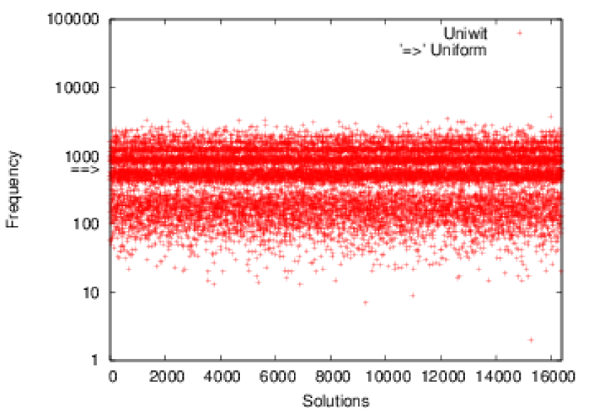
Figure 1: Sampling by $\mathsf{UniWit}$ (k=2)

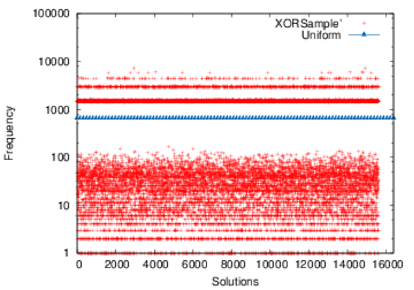
Figure 2: Sampling by $\mathsf{XORSample}^{\prime}$

As an illustration of the difference in uniformity of witnesses generated by $\mathsf{UniWit}$ and $\mathsf{XORSample}^{\prime}$, Figures 2 and 2 depict the frequencies of appearance of various witnesses using these two algorithms for an input CNF formula (case110) with $287$ variables and $16,384$ satisfying assignments. The horizontal axis in each figure represents witnesses numbered suitably, while the vertical axis represents the generated frequencies of witnesses. The frequencies were obtained from $10.8\times 10^{6}$ successful runs of each algorithm. Interestingly, $\mathsf{XORSample}^{\prime}$ could find only $15,612$ solutions (note the empty vertical band at the right end of Figure 2), while $\mathsf{UniWit}$ found all $16,384$ solutions. Further, $\mathsf{XORSample}^{\prime}$ generated each of $15$ solutions more than $5,500$ times, and more than $250$ solutions were generated only once. No such major deviations from uniformity were however observed in the frequencies generated by $\mathsf{UniWit}$. We also found that $15624$ out of $16384$ (i.e. $95.36\%$) witnesses generated by $\mathsf{UniWit}$ had frequencies in excess of $N_{unif}/8$, where $N_{unif}=10.8\times 10^{6}/16384\approx 659$. In contrast, only $6047$ (i.e. $36.91\%$) witnesses generated by $\mathsf{XORSample}^{\prime}$ had frequencies in excess of $N_{unif}/8$.

6 Concluding Remarks

We described $\mathsf{UniWit}$, an algorithm that near-uniformly samples random witnesses of Boolean formulas. We showed that the algorithm scales to reasonably large problems. We also showed that it performs better, in terms of both run time and uniformity, than previous best-of-breed algorithms for this problem. The theoretical guarantees can be further improved with higher independence of the family of hash functions used in $\mathsf{UniWit}$ (see http://www.cfdvs.iitb.ac.in/reports/reports/CAV13/ for details).

We have yet to fully explore the parameter space and the effect of pseudorandom generators other than HotBits for $\mathsf{UniWit}$. There is a trade off between failure probability, time for first witness, and time for subsequent witnesses. During our experiments, we observed the acute dearth of benchmarks available in the public domain for this important problem. We hope that our work will lead to development of benchmarks for this problem. Our focus here has been on Boolean constraints, which play a prominent role in hardware design. Extending the algorithm to handle user-provided biases would be an interesting direction of future work. Yet another interesting extension would be to consider richer constraint languages and build a uniform generator of witnesses modulo theories, leveraging recent progress in satisfiability modulo theories, c.f., [10].

References

- [1] CryptoMiniSAT. http://www.msoos.org/cryptominisat2/.
- [2] HotBits. http://www.fourmilab.ch/hotbits.
- [3] SMTLib. http://goedel.cs.uiowa.edu/smtlib/.
- [4] F. Bacchus, S. Dalmao, and T. Pitassi. Algorithms and complexity results for #SAT and Bayesian inference. In Proc. of FOCS, pages 340–351, 2003.
- [5] M. Bellare, O. Goldreich, and E. Petrank. Uniform generation of NP-witnesses using an NP-oracle. Information and Computation, 163(2):510–526, 1998.
- [6] B. Bentley. Validating a modern microprocessor. In Proc. of CAV, pages 2–4, 2005.
- [7] A.K. Chandra and V.S. Iyengar. Constraint solving for test case generation: A technique for high-level design verification. In Proc. of ICCD, pages 245 –248, 1992.
- [8] K. Chang, I.L. Markov, and V. Bertacco. Functional Design Errors in Digital Circuits: Diagnosis Correction and Repair. Springer, 2008.
- [9] A. Darwiche. A compiler for deterministic, decomposable negation normal form. In Proc. of AAAI, pages 627–634, 2002.
- [10] L.M. de Moura and N. Bjørner. Satisfiability Modulo Theories: Introduction and Applications. Commun. ACM, 54(9):69–77, 2011.
- [11] C.P. Gomes, A. Sabharwal, and B. Selman. Model counting: A new strategy for obtaining good bounds. In Proc. of AAAI, pages 54–61, 2006.
- [12] C.P. Gomes, A. Sabharwal, and B. Selman. Near-Uniform sampling of combinatorial spaces using XOR constraints. In Proc. of NIPS., pages 670–676, 2007.
- [13] E. Guralnik, M. Aharoni, A.J. Birnbaum, and A. Koyfman. Simulation-based verification of floating-point division. IEEE Trans. on Computers, 60(2):176–188, 2011.
- [14] M.R. Jerrum, L.G. Valiant, and V.V. Vazirani. Random generation of combinatorial structures from a uniform distribution. Theoretical Computer Science, 43(2-3):169–188, 1986.
- [15] S. Kirkpatrick, C. D. Gelatt, and M. P. Vecchi. Optimization by simulated annealing. Science, 220(4598):671–680, 1983.
- [16] N. Kitchen and A. Kuehlmann. Stimulus generation for constrained random simulation. In Proc. of ICCAD, pages 258–265, 2007.
- [17] Y. Mansour, N. Nisan, and P. Tiwari. The computational complexity of universal hashing. Theoretical Computer Science, 107(1):235–243, 2002.
- [18] Y. Naveh, M. Rimon, I. Jaeger, Y. Katz, M. Vinov, E. Marcus, and G. Shurek. Constraint-based random stimuli generation for hardware verification. In Proc. of AAAI, pages 1720–1727, 2006.
- [19] D. Roth. On the hardness of approximate reasoning. Artificial Intelligence, 82(1):273–302, April 1996.
- [20] M. Sipser. A complexity theoretic approach to randomness. In Proc. of STOC, pages 330–335, 1983.
- [21] L. Stockmeyer. The complexity of approximate counting. In Proc. of STOC, pages 118–126, 1983.
- [22] W. Wei, J. Erenrich, and B. Selman. Towards efficient sampling: Exploiting random walk strategies. In Proc. of AAAI, pages 670–676, 2004.
- [23] J. Yuan, A. Aziz, C. Pixley, and K. Albin. Simplifying boolean constraint solving for random simulation-vector generation. IEEE Trans. on CAD of Integrated Circuits and Systems, 23(3):412–420, 2004.