Operator folding and matrix product states in linearly-coupled bosonic arrays

Abstract

A protocol to obtain the matrix product state representation of a class of boson states is introduced. The proposal is presented in the context of linear systems and is tested by performing simulations of a reference model. The method can be applied regardless of the details of the coupling among modes and can be used to extract the most significant contribution of the tensorial representation. Characteristic issues as well as potential variants of the proposed protocol are discussed.

I Introduction

The realization that quantum states can be written in terms of a tensor network whose elements display interesting properties has prompted a wealth of research in what is nowadays known as the field of Matrix Product State (MPS) Ulrich . Although the properties of MPS can be exploited in a variety of ways, it is Time Evolving Block Decimation (TEBD) and Density Matrix Renormalization Group (DMRG), together with their variants, that have proved highly robust and appropriate in most situations of interest. However, other methods have also been proposed, for example, in the area of infinite chains, where the calculation of local mean values can be formulated in terms of bundled tensor networks, or in the area of Gaussian states, where the MPS network is obtained as projections of highly entangled states Cirac1 . MPS offers a view that is particularly convenient in variational approaches, where some physical state is obtained by renormalizing a tensor network. This has led to an interest in classes of states that can be efficiently simulated Evenbly . Notwithstanding its recurrent use in spin models, the relevance of MPS is especially notorious in bosonic systems. In this context, the application of TEBD has allowed the numerical exploration of boson chains under different conditions Reslen2 ; Danshita ; Muth ; Lacki ; Hu revealing phases and regimes with very interesting properties.

Perhaps the most elementary way of representing a quantum state is as a set of complex coefficients derived by writing such a state as a superposition of elements of a basis. In what respects to indistinguishable particles, the basis is constituted by occupation states upon which ladder operators can raise or lower the associated number of particles. Because any of these states can be put in terms of ladder operators acting on the vacuum, it is possible to envisage a representation relative to such operators. This approach is practical, for example, when the symmetries of the problem allow an advantageous handling of the Heisenberg equations Prior . This is seen in linear systems where the underlying physics is driven by interference and single body (SB) effects. These systems are quite recurrent, not only as realistic descriptions of physical phenomena, such as optical fields Buzek or weakly-interacting Bose-Einstein condensates, but also as modeling tools. The latter case is manifest, for instance, in the framework of the mean field or Hartree-Fock approximation. Insight in this direction must therefore be of significance

In the development that follows, a method is proposed to go from a representation of a bosonic state in terms of operators to a canonical MPS representation. The analysis makes use of the properties of both representations and the central argument does not involve approximations. Results obtained using the proposed technique are compared against benchmark data. It is pointed out that the range of applicability does not depend on boundary conditions or number of next-neighbors, but rather on whether the state can be put in a compatible form. In the final part, potential applications and complementary remarks are set forth.

II Linear bosonic systems

Following a second quantization scheme, let us propose a system of $M$ bosons. Every boson can occupy $N$ quantum levels which are characterized by the bosonic operators $\hat{a}_{j}$ and $\hat{a}_{k}^{\dagger}$ satisfying $[\hat{a}_{j},\hat{a}_{k}^{\dagger}]=\delta_{j}^{k}$ and $[\hat{a}_{j},\hat{a}_{k}]=0$ with $j,k=1,2,...,N$. In absence of interaction, the Hamiltonian can be written as

$$\hat{H}=\sum_{j=1}^{N}\sum_{k=1}^{N}h_{j,k}\hat{a}_{j}^{\dagger}\hat{a}_{k},\text{ }h_{j,k}=h_{k,j}^{*}.$$ (1)

Matrix $h_{j,k}$ ($\hat{h}$) is the Hamiltonian when $M=1$. $\hat{h}$ also defines the operator dynamics according to

$$\frac{d\hat{\alpha}_{j}^{\dagger}}{dt}=-i\sum_{k=1}^{N}h_{j,k}\hat{\alpha}_{k}^{\dagger},$$ (2)

which can be obtained by differentiation of $\hat{\alpha}_{j}^{\dagger}=e^{-it\hat{H}}\hat{a}_{j}^{\dagger}e^{it\hat{H}}$ ($\hbar=1$). A product of local Fock states $|n_{1},n_{2},...,n_{N}\rangle$, for which $n_{1}+n_{2}+...+n_{N}=M$, evolves as

$$|\psi(t)\rangle=\prod_{q=1}^{N}\frac{\left(\hat{\alpha}_{q}^{\dagger}\right)^{n_{q}}}{\sqrt{n_{q}!}}|0\rangle,$$ (3)

where $|0\rangle$ is the state with no bosons. More complex configurations can be constructed as superposition of these states. Now let $\epsilon_{l}$ be an eigenvalue of $\hat{h}$ corresponding to the normalized eigenstate $|\epsilon_{l}\rangle$

$$\sum_{k=1}^{N}h_{j,k}\epsilon_{k,l}=\epsilon_{l}\epsilon_{j,l}\text{ }(l,j=1,2,...,N).$$ (4)

An eigenstate $|E_{n_{1}...n_{N}}\rangle$ of $\hat{H}$ with eigenenergy $E_{n_{1}...n_{N}}=n_{1}\epsilon_{1}+n_{2}\epsilon_{2}+...+n_{N}\epsilon_{N}$ can be built as a product of SB eigenmodes as

$$|E_{n_{1}...n_{N}}\rangle=\prod_{q=1}^{N}\frac{1}{\sqrt{n_{q}!}}\left(\sum_{j=1}^{N}\epsilon_{j,q}\hat{a}_{j}^{\dagger}\right)^{n_{q}}|0\rangle.$$ (5)

The size of the basis is $(N+M-1)!/M!(N-1)!$. It can be seen that the state of a system of free bosons is determined fundamentally by the contribution of the SB Hamiltonian and the interference effects arising from indistinguishability, which is implicit in the bosonic operators. This characteristic renders the system into a linear regime, where a composition of solutions of $\hat{H}$, like in Eq. (5), is also a solution, and a SB eigenmode remains physically unaffected by other SB eigenmodes.

III Bosonic states in MPS form

In order to establish a ground to perform the transition to MPS, let us imagine that bosons are arranged in a chain with open boundary conditions. This assumption however does not need to coincide with the real boundary conditions of the problem. A site in the chain is labeled by the integer $n$ ranging from $1$ in the right end to $N$ in the left end. Using MPS, the quantum state can be represented as a superposition of non-local states in the following way (up to few changes, the notation in Vidal is followed)

$$|\psi\rangle=\sum_{\mu\nu p}\lambda_{\nu}^{[n]}\Gamma_{\nu,\mu}^{[n]}(p)\lambda_{\mu}^{[n-1]}|\nu^{[N:n+1]}\rangle|p^{[n]}\rangle|\mu^{[n-1:1]}\rangle.$$ (6)

$|\mu^{[n-1:1]}\rangle$ and $|\nu^{[N:n+1]}\rangle$ are, in that order, Schmidt vectors to the right and left of site $n$ (superscripts indicate the vector subspace). Notice that on each case such Schmidt vectors belong to different decompositions of the chain. $\lambda_{\mu}^{[n-1]}$ and $\lambda_{\nu}^{[n]}$ are the Schmidt coefficients associated to such decompositions. The states $|p^{[n]}\rangle$ are elements of a local basis at site $n$. For bosons, it is convenient to choose a local Fock basis. The complex coefficient $\Gamma_{\nu,\mu}^{[n]}(p)$ determines the contribution of a basis state to the superposition. Integer $p$ is an occupation number and ranges from $0$ to $M$. Integers $\mu$ and $\nu$ are labels of two distinct sets of Schmidt vectors. The maximum number of these vectors over all possible bipartite decompositions of the chain is called $\chi$. An important aspect of the MPS representation is that by adjusting $\chi$ it is possible to control the number of coefficients employed to describe the state. This allows to approximate huge states by retaining the most significant contribution of their respective MPS representations (the part linked to the biggest $\lambda$s). The set of tensors $\{\Gamma_{\nu,\mu}^{[n]}(p),\lambda_{\mu}^{[n]}.\forall(\mu,\nu,p,n)\}$ is a representation of $|\psi\rangle$ that can be updated when an unitary transformation is applied on a pair of consecutive sites. In what follows, it is shown how this feature can be applied to put states like (3) or (5) in MPS form.

Let us start by considering the simplified case where $n_{1}$ bosons occupy the same arbitrary SB state. The state can then be written in terms of a non-diagonal mode (NDM) as

$$|\psi\rangle=\frac{1}{\sqrt{n_{1}!}}\left(c_{1,1}\hat{a}_{1}^{\dagger}+c_{2,1}\hat{a}_{2}^{\dagger}+...+c_{N,1}\hat{a}_{N}^{\dagger}\right)^{n_{1}}|0\rangle.$$ (7)

The meaning of the second subscript in the coefficients is explained further down. Normalization of $|\psi\rangle$ requires

$$\sum_{j=1}^{N}|c_{j,1}|^{2}=1.$$ (8)

In a first step all these coefficients are to be made real. The idea is to operate on $|\psi\rangle$ with a series of local unitary transformations that act on the operators and take away the complex phases of the coefficients as follows

$$e^{-i\phi_{l,1}\hat{a}_{l}^{\dagger}\hat{a}_{l}}\hat{a}_{l}^{\dagger}e^{i\phi_{l,1}\hat{a}_{l}^{\dagger}\hat{a}_{l}}=e^{-i\phi_{l,1}}\hat{a}_{l}^{\dagger}\Rightarrow c_{l,1}\rightarrow|c_{l,1}|,$$ (9)

where $\phi_{l,1}$ is the phase of $c_{l,1}$. This is done for $l=1,2,...,N$. The order in which the transformations are applied is not important. Next, a rotation operation is applied on a couple of neighbor sites using the angular momentum operator

$$\hat{J}_{j+1,j}^{y}=\frac{1}{2i}\left(\hat{a}_{j+1}^{\dagger}\hat{a}_{j}-\hat{a}_{j}^{\dagger}\hat{a}_{j+1}\right).$$ (10)

Explicitly, this transformation reads,

$$e^{-i\theta_{j,1}\hat{J}_{j+1,j}^{y}}\left(|c_{j+1,1}|\hat{a}_{j+1}^{\dagger}+|c_{j,1}|\hat{a}_{j}^{\dagger}\right)e^{i\theta_{j,1}\hat{J}_{j+1,j}^{y}}$$

$$=\left(|c_{j+1,1}|\cos\left(\frac{\theta_{j,1}}{2}\right)-|c_{j,1}|\sin\left(\frac{\theta_{j,1}}{2}\right)\right)\hat{a}_{j+1}^{\dagger}$$

$$+\left(|c_{j+1,1}|\sin\left(\frac{\theta_{j,1}}{2}\right)+|c_{j,1}|\cos\left(\frac{\theta_{j,1}}{2}\right)\right)\hat{a}_{j}^{\dagger}.$$ (11)

Consequently, the contribution of $\hat{a}_{j+1}^{\dagger}$ can always be suppressed by choosing the appropriate angle, namely,

$$\tan\left(\frac{\theta_{j,1}}{2}\right)=\frac{|c_{j+1,1}|}{|c_{j,1}|}.$$ (12)

If the procedure is first utilized to suppress $\hat{a}_{N}^{\dagger}$, then one can successively suppress the other ladder operators in decreasing order until just $(\hat{a}_{1}^{\dagger})^{n_{1}}$ is left acting on $|0\rangle$. Here, this process is referred to as Folding. The inverse process, or Unfolding, is just a way of getting the original state back

$$|\psi\rangle=\left(\prod_{l=1}^{N}e^{i\phi_{l,1}\hat{a}_{l}^{\dagger}\hat{a}_{l}}\prod_{j=1}^{N-1}e^{i\theta_{j,1}\hat{J}_{j+1,j}^{y}}\right)\frac{\left(\hat{a}_{1}^{\dagger}\right)^{n_{1}}}{\sqrt{n_{1}!}}|0\rangle.$$ (13)

Notice that now the order in which two-site transformations are applied matters. The order of multiplication is assumed to be

$$\prod_{j=1}^{N-1}e^{i\theta_{j,1}\hat{J}_{j+1,j}^{y}}=e^{i\theta_{N-1,1}\hat{J}_{N,N-1}^{y}}\dots e^{i\theta_{1,1}\hat{J}_{2,1}^{y}},$$ (14)

and analogously in subsequent expressions. The second subscript in the angles and the coefficients makes reference to the only mode left after Folding. In order to write (13) as a set of tensors, the state with $n_{1}$ bosons in the first place of the chain is written as MPS. This can be readily done because the Schmidt vectors of such a state have a simple structure. Subsequently, the tensorial representation is updated according to Eq. (13), following the protocols available for one- and two site operations Vidal .

More complex situations take place when bosons are distributed over several SB states. As has been seen, an important class of these states can be generically represented as

$$\frac{1}{\sqrt{n_{1}!...n_{N^{\prime}}!}}\left(\sum_{k=1}^{N}c_{k,N^{\prime}}\hat{a}_{k}^{\dagger}\right)^{n_{N^{\prime}}}\dots\left(\sum_{j=1}^{N}c_{j,1}\hat{a}_{j}^{\dagger}\right)^{n_{1}}|0\rangle,$$ (15)

together with

$$\sum_{j=1}^{N}c_{j,l^{\prime}}c_{j,l}^{*}=\delta_{l^{\prime}}^{l}\text{ }(l,l^{\prime}=1,\dots,N^{\prime}),$$ (16)

which requires $N^{\prime}\leq N$. To fold (15), the first NDM is folded as shown for (7). This affect the coefficients of the other NDMs but because the transformations are linear in the operators, the new coefficients obey a relation like (16). As a result, after folding the first NDM, the coefficients of $\hat{a}_{1}^{\dagger}$ automatically vanish in the other NDMs. The process can then be applied again to fold the second NDM, but this time it is more reasonable to fold until $\hat{a}_{2}^{\dagger}$ is left alone, skipping the last folding operation, since $\hat{a}_{1}^{\dagger}$ is not present in the second NDM. In this way, folding the second NDM does not unfold the first mode and $\hat{a}_{2}^{\dagger}$ disappears from the rest of NDMs. The procedure is repeated in a similar way until the state is reduced to a simple product of local Fock states. The original state (15) can therefore be recovered as

$$\left(\prod_{k=N^{\prime}}^{1}\left(\prod_{l=k}^{N}e^{i\phi_{l,k}\hat{a}_{l}^{\dagger}\hat{a}_{l}}\prod_{j=k}^{N-1}e^{i\theta_{j,k}\hat{J}_{j+1,j}^{y}}\right)\right)\prod_{q=1}^{N^{\prime}}\frac{\left(\hat{a}_{q}^{\dagger}\right)^{n_{q}}}{\sqrt{n_{q}!}}|0\rangle,$$ (17)

which in turn can be numerically implemented in terms of MPS as explained before.

IV Applications

In order to test Unfolding in a controlled manner, a Hamiltonian with a known analytical profile is brought up, namely

$$h_{j,k}=\delta_{k+1}^{j}+\delta_{k}^{j+1},$$ (18)

plus periodic boundary conditions, $h_{j,N+1}=h_{j,1}$ and $h_{N+1,k}=h_{1,k}$ ($\hat{a}_{N+1}^{\dagger}=\hat{a}_{1}^{\dagger}$). As the spectrum of this Hamiltonian is in general degenerate, the next reference eigensystem is chosen

$$\epsilon_{l}=2\cos\left(\frac{2\pi l}{N}\right),\text{ }\epsilon_{k,l}=\frac{e^{2\pi kli/N}}{\sqrt{N}}.$$ (19)

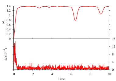
Figure 1: Entropy between one site and the rest of the system (Top) and error $\Delta=1-|\langle\psi|\psi^{\prime}\rangle|^{2}$ (Bottom) in a boson chain with $N=8$ and $M=8$ initialized with one particle at each site. The underlying Hamiltonian displays next-neighbor hopping (Eqs. (1) and (18)) and the boundary conditions are periodic. The error determines the difference between the state found by standard diagonalization ($|\psi^{\prime}\rangle$) and by Unfolding as explained in the text.

The calculation consists in solving Eq. (2) and then inserting the dynamical operators in Eq. (3), assuming that at $t=0$ there is one boson at each site of the chain. The resulting state is then written as a tensor network using Unfolding. To do this, Eq. (17) is implemented as a numerical routine that integrates the updating subroutine of the programs described in Reslen2 . The obtained results are then compared against equivalent simulations carried by diagonalization. The lower panel of Fig. 1 shows, as a function of time, the numerical error produced by Unfolding when compared to the standard method. Unless otherwise stated, it must be assumed that in the MPS computations $\chi$ is not bounded but dynamically determined by the updating routine as the simulation runs. In this way, all the elements of the MPS representation are retained. As can be seen in Fig. 1, error is comparable to computer precision and it does not grow over long intervals. This because in Unfolding the state for a given time only depends on the initial condition and the solution of the equations of motion for the operators, which can be obtained with high accuracy for any $t$. The upper panel of Fig. 1 shows the single site entropy of the chain, calculated from

$$S=-\sum_{\mu}\left(\lambda_{\mu}^{[1]}\right)^{2}\log\left(\lambda_{\mu}^{[1]}\right)^{2}.$$ (20)

$S$ measures the entanglement between one site and the rest of the chain and can be easily computed from a MPS representation. It is known that the chain relaxes to a Gaussian state with maximum entropy subject to fixed second moments Cramer . As a result, the saturation of $S$ determines a time window along which the dynamics is relevant.

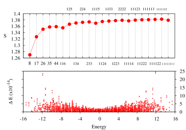
Figure 2: Entropy between one site and the rest of the system (Top) and error $\Delta E=|E-E_{n_{1},\dots,n_{N}}|$ (Bottom) of energy eigenstates of Hamiltonian (1) for $N=8$ and $M=8$. The eigenstates are built as products of SB eigenmodes, as described by Eq. (5), and then converted to MPS in order to find $S$ and $E$. Since $S$ depends only on the exponents of the product, a many-particle state is represented by the number of bosons at each SB state, making no reference to which SB state the exponent actually apply. For instance, $17$ means two SB states are involved, the first with $1$ boson and the second with $7$ bosons. Entropy is independent on the specific choice of such SB states.

Fig. 2 shows $S$ for the eigenstates of $\hat{H}$ as well as the numerical error incurred by passing such eigenstates to MPS using Unfolding. In this figure every state has been represented only by the exponents that appear in Eq. (5). This can be done because a SB eigenmode formed from (19) can be transformed into any other SB eigenmode of the same family using only single-site unitary operations. Recall that invariance under local unitary transformations is a property of entanglement. Fig. 2 suggests that eigenstates of $\hat{H}$ made of bosons distributed over many SB eigenstates contain more entanglement than eigenstates with bosons arranged over few SB eigenstates. Nevertheless, the eigenstate of $\hat{H}$ with all SB states occupied does not show maximum entanglement.

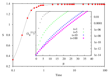
Figure 3: Boson chain with $N=100$, $M=100$ and the same conditions as in Fig. 1. In this example the size of the MPS representation was bounded by setting $\chi=50$. Inset. Eigenvalues of the single-site density matrix for different times. As the logarithmic plot of the eigenvalue distribution becomes more linear, the state approaches a Gaussian state.

The efficiency of Unfolding as a numerical method varies inversely to $\chi$. In relation to this, the number of operations necessary to update the MPS representation every time a unitary transformation is applied grows with the size of the local basis ($M+1$), but is attenuated by exploiting conservation of number of particles. Moreover, from the arguments in Vidal it follows that the number of operations required to update the state must grow as a polynomial of $\chi$. This makes Unfolding suitable for systems with little entanglement. However, because every time the state is computed only one round of unitary operations is invoked (Eq. 17), Unfolding is different to methods where the calculation of the state for a given time entails an integration of short evolutions. The fact that in Unfolding error does not accumulate with time is also an advantage, as well as the fact that specific choices of boundary conditions or number of neighbors do not necessarily preclude the application of the method. The key point is to put the state in the form of Eq. (15). Likewise, the advantages of Unfolding over diagonalization can be appreciated by noticing that while the basis of $\hat{H}$ grows exponentially with $N$, the bases of the matrices involved in the Unfolding calculation grow linearly with $N$. In comparison to other methods that could be applied in the same circumstances, Unfolding would be suitable when a MPS description is preferred or when entanglement is small.

For states with large entanglement, Unfolding can be used to get an estimation. This is done by setting $\chi$ to a numerically manageable value. Fig. 3 shows some results obtained by fixing $\chi$ in a simulation of a relatively big chain. In spite of the approximation, the relaxation profile shows good agreement with theoretical assessments reported in Cramer .

V Discussion and outline

Although Unfolding has been presented in the context of a specific class of initial states, it appears the same strategies can in principle be applied whenever the state is in general given by

$$f\left(\sum_{k=1}^{N}c_{k,N^{\prime}}\hat{a}_{k}^{\dagger},\dots,\sum_{j=1}^{N}c_{j,1}\hat{a}_{j}^{\dagger}\right)|0\rangle,$$ (21)

as long as $f$ could be expanded in Taylor series. Furthermore, coherent states like

$$e^{\sum_{j}\alpha_{j}\hat{a}_{j}^{\dagger}-\alpha_{j}^{*}\hat{a}_{j}}|0\rangle,$$ (22)

exhibit some compatibility with Unfolding too. In these cases, Folding would reduce the state to a function of ladder operators acting on $|0\rangle$. The success of the method would then depend on the possibility of writing such a reduced state in MPS terms without much effort. The translated state can then be used as the initial condition in a simulation effectuated by, for instance, TEBD.

As commutativity of NDMs (Eq. (16)) is assumed in Unfolding, non-commuting NDMs can be treated by adding modes that correct this anomaly. As an example, consider the state

$$\left(\sum_{j=1}^{2}c_{j,1}\hat{a}_{j}^{\dagger}\right)\left(\sum_{k=1}^{2}c_{k,2}\hat{a}_{k}^{\dagger}\right)|0\rangle,\text{ }\sum_{j=1}^{2}c_{j,1}c_{j,2}^{*}\neq 0.$$ (23)

A third mode can be introduced so that

$$\left(\sum_{j=1}^{3}c_{j,1}\hat{a}_{j}^{\dagger}\right)\left(\sum_{k=1}^{3}c_{k,2}\hat{a}_{k}^{\dagger}\right)|0\rangle,\text{ }\sum_{j=1}^{3}c_{j,1}c_{j,2}^{*}=0.$$ (24)

Up to a normalization constant, the new state can be folded as shown above. Once the transformation to MPS has been carried, the coefficients related to the extra mode can be dropped. This approach is resembling of density matrix purification. On the other hand, one way of taking interaction effects into account is to apply perturbation theory, treating non-linear terms as perturbations. This would result especially effective when the non-linearity is local, because the MPS description is appropriate to find local mean values. Another way is to mimic the interaction using a mean-field approach. This could be realized by using the solution of the non-linear Gross-Pitaevskii equation as the coefficients of Eq. (7). One can also think of using Eq. (17) as a variational ansatz, similar to the Gutzwiller ansatz.

An alternative method has been proposed in the context of linear bosonic systems to compute physical quantum states in MPS form. The technique has been used to simulate an understood model and the results have been compared against both data produced by diagonalization and theoretical studies. Agreement has been satisfactory in every case. Aspects related to the suitability and scope of the technique have been analyzed and complementary observations have been made.

References

- (1) U. Schollwöck, Annals of Phys. 326 96 (2011).
- (2) M.C. Bañuls, M.B. Hastings, F. Verstraete and J.I. Cirac, Phys. Rev. Lett. 102 240603 (2009), N. Schuch, M.M. Wolf and J.I. Cirac, arXiv:1201.3945.
- (3) G. Evenbly and G. Vidal, New J. Phys. 12 025007 (2010), G. Evenbly and G. Vidal, arXiv:1210:1895.
- (4) R.V. Mishmash, I. Danshita, C.W. Clark, L.D. Carr, Phys. Rev. A 80 053612 (2009).
- (5) D. Muth and M. Fleischhauer, Phys. Rev. Lett. 105 150403 (2010).
- (6) A. Hu, L. Mathey, C.J. Williams and C.W. Clark, Phys. Rev. A 81 063602 (2010).
- (7) M. Lacki, D. Delande and J. Zakrzewski, Phys. Rev. A 86 013602 (2012).
- (8) J. Reslen and S. Bose, Phys. Rev. A 80, 012330 (2009), J. Reslen, arXiv:1002.4001.
- (9) S.R. Clark, J. Prior, M.J. Hartmann, D. Jaksch and M.B. Plenio, New J. Phys. 12 025005 (2010).
- (10) M.S. Kim, W. Son, V. Buzek and P.L. Knight, Phys. Rev. A 65 032323 (2002).
- (11) G. Vidal, Phys. Rev. Lett. 91, 147902 (2003).
- (12) M. Cramer, C.M. Dawson, J. Eisert and T.J. Osborne, Phys. Rev. Lett. 100, 030602 (2008).