Data enriched linear regression

Abstract

We present a linear regression method for predictions on a small data set making use of a second possibly biased data set that may be much larger. Our method fits linear regressions to the two data sets while penalizing the difference between predictions made by those two models. The resulting algorithm is a shrinkage method similar to those used in small area estimation. We find a Stein-type finding for Gaussian responses: when the model has $5$ or more coefficients and $10$ or more error degrees of freedom, it becomes inadmissible to use only the small data set, no matter how large the bias is. We also present both plug-in and AICc-based methods to tune our penalty parameter. Most of our results use an $L_{2}$ penalty, but we obtain formulas for $L_{1}$ penalized estimates when the model is specialized to the location setting. Ordinary Stein shrinkage provides an inadmissibility result for only $3$ or more coefficients, but we find that our shrinkage method typically produces much lower squared errors in as few as $5$ or $10$ dimensions when the bias is small and essentially equivalent squared errors when the bias is large.

arXiv:0000.0000

, and

t1Art Owen worked on this project as a consultant for Google; it was not part of his Stanford responsibilities.

1 Introduction

The problem we consider here is how to combine linear regressions based on data from two sources. There is a small data set of expensive high quality observations and a possibly much larger data set with less costly observations. The big data set is thought to have similar but not identical statistical characteristics to the small one. The conditional expectation might be different there or the predictor variables might have been measured in somewhat different ways. The motivating application comes from within Google. The small data set is a panel of consumers, selected by a probability sample, who are paid to share their internet viewing data along with other data on television viewing. There is a second and potentially much larger panel, not selected by a probability sample who have opted in to the data collection process.

The goal is to make predictions for the population from which the smaller sample was drawn. If the data are identically distributed in both samples, we should simply pool them. If the big data set is completely different from the small one, then using it may not be worth the trouble.

Many settings are intermediate between these extremes: the big data set is similar but not necessarily identical to the small one. We stand to benefit from using the big data set at the risk of introducing some bias. Our goal is to glean some information from the larger data set to increase accuracy for the smaller one. The difficulty is that our best information about how the two populations are similar is in our samples from them.

The motivating problem at Google has some differences from the problem we consider here. There were two binary responses, one sample was missing one of those responses, and tree-based predictions were used. See Chen et al., (2014). This paper studies linear regression because it is more amenable to theoretical analysis, is more fundamental, and sharper statements are possible.

The linear regression method we use is a hybrid between simply pooling the two data sets and fitting separate models to them. As explained in more detail below, we apply shrinkage methods penalizing the difference between the regression coefficients for the two data sets. Both the specific penalties we use, and our tuning strategies, reflect our greater interest in the small data set. Our goal is to enrich the analysis of the smaller data set using possibly biased data from the larger one.

Section 2 presents our notation and introduces $L_{1}$ and $L_{2}$ penalties on the parameter difference. Most of our results are for the $L_{2}$ penalty. For the $L_{2}$ penalty, the resulting estimate is a linear combination of the two within sample estimates. Theorem 2.1 gives a formula for the degrees of freedom of that estimate. Theorem 2.2 presents the mean squared error of the estimator and forms the basis for plug-in estimation of an oracle’s value when an $L_{2}$ penalty is used. We also show how to use Stein shrinkage, shrinking the regression coefficient in the small sample towards the estimate from the large sample. Such shrinkage makes it inadmissible to ignore the large sample when there are $3$ or more coefficients including the intercept.

Section 3 considers in detail the case where the regression simplifies to estimation of a population mean. In that setting, we can determine how plug-in, bootstrap and cross-validation estimates of tuning parameters behave. We get an expression for how much information the large sample can add. Theorem 3.1 gives a soft-thresholding expression for the estimate produced by $L_{1}$ penalization and equation (3.7) can be used to find the penalty parameter that an $L_{1}$ oracle would choose when the data are Gaussian.

Section 4 presents some simulated examples. We simulate the location problem for several $L_{2}$ penalty methods varying in how aggressively they use the larger sample. The $L_{1}$ oracle is outperformed by the $L_{2}$ oracle in this setting. When the bias is small, the data enrichment methods improve upon the small sample, but when the bias is large then it is best to use the small sample only. Things change when we simulate the regression model. For dimension $d\geq 5$, data enrichment outperforms the small sample method in our simulations at all bias levels. We did not see such an inadmissibility outcome when we simulated cases with $d\leq 4$. In our simulated examples, the data enrichment estimator performs better than plain Stein shrinkage of the small sample towards the large sample.

Section 5 presents theoretical support for our estimator. Theorem 5.1. shows that when there are $5$ or more predictors and $10$ or more degrees of freedom for error, then some of our data enrichment estimators make simply using the small sample inadmissible. The reduction in mean squared error is greatest when the bias is smallest, but no matter how large the bias is, we gain an improvement. The estimator we study employs a data-driven weighting of the two within-sample least squares estimators. In simulations, our plug-in estimator performed even better than the estimator from Theorem 5.1. Section 6 explains how our estimators are closer to a matrix oracle than the James-Stein estimators are, and this may explain why they outperform simple shrinkage in our simulations.

There are many statistical settings where data from one setting is used to study a different setting. They range from older methods in survey sampling, to recently developed methods for bioinformatics. Section 7 surveys some of those literatures. Section 8 has brief conclusions. The longer proofs are in Section 9 of the Appendix.

Our contributions include the following:

• a new penalization method for combining data sets,

• an inadmissibility result based on that method,

• a comparison of $L_{1}$ and $L_{2}$ penalty oracles for the location setting, and

• evidence that more aggressive shrinkage pays in high dimensions.

2 Data enriched regression

Consider linear regression with a response $Y\in\mathbb{R}$ and predictors $X\in\mathbb{R}^{d}$. The model for the small data set is

$$Y_{i}=X_{i}\beta+\varepsilon_{i},\quad i\in S$$

for a parameter $\beta\in\mathbb{R}^{d}$ and independent errors $\varepsilon_{i}$ with mean $0$ and variance $\sigma_{S}^{2}$. Now suppose that the data in the big data set follow

$$Y_{i}=X_{i}(\beta+\gamma)+\varepsilon_{i},\quad i\in B$$

where $\gamma\in\mathbb{R}^{d}$ is a bias parameter and $\varepsilon_{i}$ are independent with mean $0$ and variance $\sigma^{2}_{B}$. The sample sizes are $n$ in the small sample and $N$ in the big sample.

There are several kinds of departures of interest. It could be, for instance, that the overall level of $Y$ is different in $S$ than in $B$ but that the trends are similar. That is, perhaps only the intercept component of $\gamma$ is nonzero. More generally, the effects of some but not all of the components in $X$ may differ in the two samples. One could apply hypothesis testing to each component of $\gamma$ but that is unattractive as the number of scenarios to test for grows as $2^{d}$.

Let $X_{S}\in\mathbb{R}^{n\times d}$ and $X_{B}\in\mathbb{R}^{N\times d}$ have rows made of vectors $X_{i}$ for $i\in S$ and $i\in B$ respectively. Similarly, let $Y_{S}\in\mathbb{R}^{n}$ and $Y_{B}\in\mathbb{R}^{N}$ be corresponding vectors of response values. We use $V_{S}=X_{S}^{\mathsf{T}}X_{S}$ and $V_{B}=X_{B}^{\mathsf{T}}X_{B}$.

2.1 Partial pooling via shrinkage and weighting

Our primary approach is to pool the data but put a shrinkage penalty on $\gamma$. We estimate $\beta$ and $\gamma$ by minimizing

$$\sum_{i\in S}(Y_{i}-X_{i}\beta)^{2}+\sum_{i\in B}(Y_{i}-X_{i}(\beta+\gamma))^{2}+\lambda P(\gamma)$$ (2.1)

where $\lambda\in[0,\infty]$ and $P(\gamma)\geq 0$ is a penalty function. There are several reasonable choices for the penalty function, including

$$\|\gamma\|_{2}^{2},\quad\|X_{S}\gamma\|_{2}^{2},\quad\|\gamma\|_{1},\quad\text{and}\quad\|X_{S}\gamma\|_{1}.$$

For each of these penalties, setting $\lambda=0$ leads to separate fits $\hat{\beta}$ and $\hat{\beta}+\hat{\gamma}$ in the two data sets. Similarly, taking $\lambda=\infty$ constrains $\hat{\gamma}=0$ and amounts to pooling the samples. We will see that varying $\lambda$ shifts the relative weight applied to the two samples. In many applications one will want to regularize $\beta$ as well, but in this paper we only penalize $\gamma$.

The criterion (2.1) does not account for different variances in the two samples. If we knew the variance ratio we might multiply the sum over $i\in B$ by $\tau=\sigma^{2}_{S}/\sigma^{2}_{B}$. A large value of $\tau$ has the consequence of increasing the weight on the $B$ sample. Choosing $\tau$ is largely confounded with choosing $\lambda$ because $\lambda$ also adjusts the relative weight of the two samples. We use $\tau=1$, but in a context with some prior knowledge about the magnitude of $\sigma^{2}_{S}/\sigma^{2}_{B}$ another value could be used. Our inadmissibility result does not depend on knowing the correct $\tau$.

The $L_{1}$ penalties have an advantage in interpretation because they identify which parameters or which specific observations might be differentially affected. The quadratic penalties are more analytically tractable, so we focus most of this paper on them.

Both quadratic penalties can be expressed as $\|X_{T}\gamma\|_{2}^{2}$ for a matrix $X_{T}$. The rows of $X_{T}$ represent a hypothetical target population of $N_{T}$ items for prediction. The matrix $V_{T}=X_{T}^{\mathsf{T}}X_{T}$ is then proportional to the matrix of mean squares and mean cross-products for predictors in the target population.

If we want to remove the pooling effect from one of the coefficients, such as the intercept term, then the corresponding column of $X_{T}$ should contain all zeros. We can also constrain $\gamma_{j}=0$ (by dropping its corresponding predictor) in order to enforce exact pooling on the $j$’th coefficient.

A second, closely related approach is to fit $\hat{\beta}_{S}$ by minimizing $\sum_{i\in S}(Y_{i}-X_{i}\beta)^{2}$, fit $\hat{\beta}_{B}$ by minimizing $\sum_{i\in B}(Y_{i}-X_{i}\beta)^{2}$, and then estimate $\beta$ by

$$\hat{\beta}(\omega)=\omega\hat{\beta}_{S}+(1-\omega)\hat{\beta}_{B}$$

for some $0\leq\omega\leq 1$. In some special cases the estimates indexed by the weighting parameter $\omega\in[n/(n+N),1]$ are a relabeling of the penalty-based estimates indexed by the parameter $\lambda\in[0,\infty]$. In other cases, the two families of estimates differ. The weighting approach allows simpler tuning methods. Although we find in simulations that the penalization method is superior, we can prove stronger results about the weighting approach.

Given two values of $\lambda$ we consider the larger one to be more ‘aggressive’ in that it makes more use of the big sample bringing with it the risk of more bias in return for a variance reduction. Similarly, aggressive estimators correspond to small weights $\omega$ on the small target sample.

2.2 Quadratic penalties and degrees of freedom

The quadratic penalty takes the form $P(\gamma)=\|X_{T}\gamma\|^{2}_{2}=\gamma^{\mathsf{T}}V_{T}\gamma$ for a matrix $X_{T}\in\mathbb{R}^{r\times d}$ and $V_{T}=X_{T}^{\mathsf{T}}X_{T}\in\mathbb{R}^{d\times d}$. The value $r$ is $d$ or $n$ in the examples above and could take other values in different contexts. Our criterion becomes

$$\|Y_{S}-X_{S}\beta\|^{2}+\|Y_{B}-X_{B}(\beta+\gamma)\|^{2}+\lambda\|X_{T}\gamma\|^{2}.$$ (2.2)

Here and below $\|x\|$ means the Euclidean norm $\|x\|_{2}$.

Given the penalty matrix $X_{T}$ and a value for $\lambda$, the penalized sum of squares (2.2) is minimized by $\hat{\beta}_{\lambda}$ and $\hat{\gamma}_{\lambda}$ satisfying

$$\mathcal{X}^{\mathsf{T}}\mathcal{X}\begin{pmatrix}\hat{\beta}_{\lambda}\\ \hat{\gamma}_{\lambda}\end{pmatrix}=\mathcal{X}^{\mathsf{T}}\mathcal{Y}$$

where

$$\mathcal{X}=\begin{pmatrix}X_{\mathrm{S}}&0\\ X_{\mathrm{B}}&X_{\mathrm{B}}\\ 0&\lambda^{1/2}X_{T}\end{pmatrix}\in\mathbb{R}^{(n+N+r)\times 2d},\quad\text{and}\quad\mathcal{Y}=\begin{pmatrix}Y_{\mathrm{S}}\\ Y_{\mathrm{B}}\\ 0\end{pmatrix}.$$ (2.3)

To avoid uninteresting complications we suppose that the matrix $\mathcal{X}^{\mathsf{T}}\mathcal{X}$ is invertible. The representation (2.3) also underlies a convenient computational approach to fitting $\hat{\beta}_{\lambda}$ and $\hat{\gamma}_{\lambda}$ using $r$ rows of pseudo-data just as one does in ridge regression.

The estimate $\hat{\beta}_{\lambda}$ can be written in terms of $\hat{\beta}_{S}=V_{S}^{-1}X_{S}^{\mathsf{T}}Y_{S}$ and $\hat{\beta}_{B}=V_{B}^{-1}X_{B}^{\mathsf{T}}Y_{B}$ as the next lemma shows.

Lemma 2.1.

Let $X_{S}$, $X_{B}$, and $X_{T}$ in (2.2) all have rank $d$. Then for any $\lambda\geq 0$, the minimizers $\hat{\beta}$ and $\hat{\gamma}$ of (2.2) satisfy

$$\hat{\beta}=W_{\lambda}\hat{\beta}_{S}+(I-W_{\lambda})\hat{\beta}_{B}$$

and $\hat{\gamma}=(V_{B}+\lambda V_{T})^{-1}V_{B}(\hat{\beta}_{B}-\hat{\beta})$ for a matrix

$$W_{\lambda}=(V_{S}+\lambda V_{T}V_{B}^{-1}V_{S}+\lambda V_{T})^{-1}(V_{S}+\lambda V_{T}V_{B}^{-1}V_{S}).$$ (2.4)

If $V_{T}=V_{S}$, then

$$W_{\lambda}=(V_{B}+\lambda V_{S}+\lambda V_{B})^{-1}(V_{B}+\lambda V_{S}).$$

Proof.

The normal equations of (2.2) are

$$(V_{B}+V_{S})\hat{\beta}=V_{S}\hat{\beta}_{S}+V_{B}\hat{\beta}_{B}-V_{B}\hat{\gamma}\quad\text{and}\quad(V_{B}+\lambda V_{T})\hat{\gamma}=V_{B}\hat{\beta}_{B}-V_{B}\hat{\beta}.$$

Solving the second equation for $\hat{\gamma}$, plugging the result into the first and solving for $\hat{\beta}$, yields the result with $W_{\lambda}=(V_{S}+V_{B}-V_{B}(V_{B}+\lambda V_{T})^{-1}V_{B})^{-1}V_{S}$. This expression for $W_{\lambda}$ simplifies as given and simplifies further when $V_{T}=V_{S}$. ∎

The remaining challenge in model fitting is to choose a value of $\lambda$. Because we are only interested in making predictions for the $S$ data, not the $B$ data, the ideal value of $\lambda$ is one that optimizes the prediction error on sample $S$. One reasonable approach is to use cross-validation by holding out a portion of sample $S$ and predicting the held-out values from a model fit to the held-in ones as well as the entire $B$ sample. One may apply either leave-one-out cross-validation or more general $K$-fold cross-validation. In the latter case, sample $S$ is split into $K$ nearly equally sized parts and predictions based on sample $B$ and $K-1$ parts of sample $S$ are used for the $K$’th held-out fold of sample $S$.

We prefer to use criteria such as AIC, AICc, or BIC in order to avoid the cost and complexity of cross-validation. To compute AIC and alternatives, we need to measure the degrees of freedom used in fitting the model. We define the degrees of freedom to be

$$\mathrm{df}(\lambda)=\frac{1}{\sigma_{S}^{2}}\sum_{i\in S}\mathrm{cov}(\hat{Y}_{i},Y_{i}),$$ (2.5)

where $\hat{Y}_{S}=X_{S}\hat{\beta}_{\lambda}$. This is the formula of Ye, (1998) and Efron, (2004) adapted to our setting where the focus is only on predictions for the $S$ data. We will see later that the resulting AIC type estimates based on the degrees of freedom perform similarly to our focused cross-validation described above.

Theorem 2.1.

For data enriched regression the degrees of freedom given at (2.5) satisfies $\mathrm{df}(\lambda)=\mathrm{tr}(W_{\lambda})$ where $W_{\lambda}$ is given in Lemma 2.1. If $V_{T}=V_{S}$, then

$$\mathrm{df}(\lambda)=\sum_{j=1}^{d}\frac{1+\lambda\nu_{j}}{1+\lambda+\lambda\nu_{j}}$$ (2.6)

where $\nu_{1},\dots,\nu_{d}$ are the eigenvalues of

$$M\equiv V_{S}^{1/2}V_{B}^{-1}V_{S}^{1/2}$$ (2.7)

in which $V_{S}^{1/2}$ is a symmetric matrix square root of $V_{S}$.

Proof.

Section 9.1 in the Appendix. ∎

With a notion of degrees of freedom customized to the data enrichment context we can now define the corresponding criteria such as

$$\text{AIC}(\lambda) =n\log(\hat{\sigma}^{2}_{S}(\lambda))+n\Bigl{(}1+\frac{2\mathrm{df}(\lambda)}{n}\Bigr{)}\quad\text{and}$$

$$\text{AICc}(\lambda) =n\log(\hat{\sigma}^{2}_{S}(\lambda))+n\Bigl{(}1+\frac{\mathrm{df}(\lambda)}{n}\Bigr{)}\Bigm{/}\Bigl{(}1-\frac{\mathrm{df}(\lambda)+2}{n}\Bigr{)},$$ (2.8)

where $\hat{\sigma}^{2}_{S}(\lambda)=(n-d)^{-1}\sum_{i\in S}^{n}(Y_{i}-X_{i}\hat{\beta}(\lambda))^{2}$. The AIC is more appropriate than BIC here since our goal is prediction accuracy, not model selection. We prefer the AICc criterion of Hurvich and Tsai, (1989) because it is more conservative as the degrees of freedom become large compared to the sample size.

Next we illustrate some special cases of the degrees of freedom formula in Theorem 2.1. First, suppose that $\lambda=0$, so that there is no penalization on $\gamma$. Then $\mathrm{df}(0)=\mathrm{tr}(I)=d$ as is appropriate for regression on sample $S$ only.

We can easily see that the degrees of freedom are monotone decreasing in $\lambda$. As $\lambda\to\infty$ the degrees of freedom drop to $\mathrm{df}(\infty)=\sum_{j=1}^{d}\nu_{j}/(1+\nu_{j})$. This can be much smaller than $d$. For instance if $V_{S}=n\Sigma$ and $V_{B}=N\Sigma$ for some positive definite $\Sigma\in\mathbb{R}^{d\times d}$, then all $\nu_{j}=n/N$ and so $\mathrm{df}(\infty)=d/(1+N/n)\leq dn/N$.

Monotonicity of the degrees of freedom makes it easy to search for the value $\lambda$ which delivers a desired degrees of freedom. We have found it useful to investigate $\lambda$ over a numerical grid corresponding to degrees of freedom decreasing from $d$ by an amount $\Delta$ (such as $0.25$) to the smallest such value above $\mathrm{df}(\infty)$. It is easy to adjoin $\lambda=\infty$ (sample pooling) to this list as well.

2.3 Predictive mean square errors

Here we develop an oracle’s choice for $\lambda$ and a corresponding plug-in estimate. We work in the case where $V_{S}=V_{T}$ and we assume that $V_{S}$ has full rank. Given $\lambda$, the predictive mean square error is $\mathbb{E}(\|X_{S}(\hat{\beta}-\beta)\|^{2})$.

We will use the matrices $V_{S}^{1/2}$ and $M$ from Theorem 2.1 and the eigendecomposition $M=UDU^{\mathsf{T}}$ where the $j$’th column of $U$ is $u_{j}$ and $D=\mathrm{diag}(\nu_{j})$.

Theorem 2.2.

The predictive mean square error of the data enrichment estimator is

$$\mathbb{E}\bigl{(}\|X_{S}(\hat{\beta}-\beta)\|^{2}\bigr{)} =\sigma_{S}^{2}\sum_{j=1}^{d}\frac{(1+\lambda\nu_{j})^{2}}{(1+\lambda+\lambda\nu_{j})^{2}}+\sum_{j=1}^{d}\frac{\lambda^{2}\kappa_{j}^{2}}{(1+\lambda+\lambda\nu_{j})^{2}}$$ (2.9)

where $\kappa_{j}^{2}={u_{j}^{\mathsf{T}}V_{S}^{1/2}\Theta V_{S}^{1/2}u_{j}}$ for $\Theta=\gamma\gamma^{T}+\sigma_{B}^{2}V_{B}^{-1}$.

Proof.

Section 9.2. ∎

The first term in (2.9) is a variance term. It equals $d\sigma^{2}_{S}$ when $\lambda=0$ but for $\lambda>0$ it is reduced due to the use of the big sample. The second term represents the error, both bias squared and variance, introduced by the big sample.

2.4 A plug-in method

A natural choice of $\lambda$ is to minimize the predictive mean square error, which must be estimated. We propose a plug-in method that replaces the unknown parameters $\sigma_{S}^{2}$ and $\kappa_{j}^{2}$ from Theorem 2.2 by sample estimates. For estimates ${\hat{\sigma}_{S}^{2}}$ and $\hat{\kappa}_{j}^{2}$ we choose

$$\hat{\lambda} =\arg\min_{\lambda\geq 0}\,\sum_{j=1}^{d}\,\frac{\hat{\sigma}_{S}^{2}(1+\lambda\nu_{j})^{2}+\lambda^{2}\hat{\kappa}_{j}^{2}}{(1+\lambda+\lambda\nu_{j})^{2}}.$$ (2.10)

From the sample data we take $\hat{\sigma}^{2}_{S}=\|Y_{S}-X_{S}\hat{\beta}_{S}\|^{2}/(n-d)$. A straightforward plug-in estimate of the matrix $\Theta$ in Theorem 2.2 is

$$\widehat{\Theta}_{\mathrm{plug}} =\hat{\gamma}\hat{\gamma}^{\mathsf{T}}+{\hat{\sigma}_{B}^{2}}V_{B}^{-1},$$

where $\hat{\gamma}=\hat{\beta}_{B}-\hat{\beta}_{S}$. Now we take $\hat{\kappa}^{2}_{j}=u_{j}^{\mathsf{T}}V_{S}^{1/2}\widehat{\Theta}V_{S}^{1/2}u_{j}$ recalling that $u_{j}$ and $\nu_{j}$ derive from the eigendecomposition of $M=V_{S}^{1/2}V_{B}^{-1}V_{S}^{1/2}$. The resulting optimization yields an estimate $\hat{\lambda}_{\mathrm{plug}}$.

The estimate $\widehat{\Theta}_{\mathrm{plug}}$ is biased upwards because $\mathbb{E}(\hat{\gamma}\hat{\gamma}^{\mathsf{T}})=\gamma\gamma^{\mathsf{T}}+\sigma^{2}_{B}V_{B}^{-1}+\sigma^{2}_{S}V_{S}^{-1}$. We have used a bias-adjusted plug-in estimate

$$\widehat{\Theta}_{\mathrm{bapi}}=\hat{\sigma}_{B}^{2}V_{B}^{-1}+(\hat{\gamma}\hat{\gamma}^{\mathsf{T}}-\hat{\sigma}_{B}^{2}V_{B}^{-1}-\hat{\sigma}_{S}^{2}V_{S}^{-1})_{+}$$ (2.11)

where the positive part operation on a symmetric matrix preserves its eigenvectors but replaces any negative eigenvalues by $0$. Similar results can be obtained with

$$\widetilde{\Theta}_{\mathrm{bapi}}=\bigl{(}\hat{\gamma}\hat{\gamma}^{\mathsf{T}}-{\hat{\sigma}_{S}^{2}}V_{S}^{-1}\bigr{)}_{+}.$$ (2.12)

This estimator is somewhat simpler but (2.11) has the advantage of being at least as large as $\hat{\sigma}^{2}_{B}V_{B}^{-1}$ while (2.12) can degenerate to $0$.

2.5 James-Stein shrinkage estimators

For background on these estimators, see Efron and Morris, 1973b . We shrink $\hat{\theta}_{S}=V_{S}^{1/2}\hat{\beta}_{S}\sim\mathcal{N}(V_{S}^{1/2}\beta,\sigma^{2}_{S}I_{n})$ towards a target vector, to get better estimators of $\theta_{S}=V_{S}^{1/2}\beta$. To make use of the big data set we shrink $\hat{\theta}_{S}$ towards

$$\hat{\theta}_{B}=V_{S}^{1/2}\hat{\beta}_{B}\sim\mathcal{N}(V_{S}^{1/2}(\beta+\gamma),V_{S}^{1/2}V_{B}^{-1}V_{S}^{1/2}\sigma^{2}_{B}).$$

We consider two shrinkers

$$\hat{\theta}_{\mathrm{JS},B} =\hat{\theta}_{B}+\Bigl{(}1-\frac{d-2}{\|\hat{\theta}_{S}-\hat{\theta}_{B}\|^{2}/\sigma^{2}_{S}}\Bigr{)}(\hat{\theta}_{S}-\hat{\theta}_{B}),\quad\text{and}$$

$$\hat{\theta}_{\mathrm{JS},B+} =\hat{\theta}_{B}+\Bigl{(}1-\frac{d-2}{\|\hat{\theta}_{S}-\hat{\theta}_{B}\|^{2}/\sigma^{2}_{S}}\Bigr{)}_{+}(\hat{\theta}_{S}-\hat{\theta}_{B}).$$ (2.13)

Each of these makes $\hat{\theta}_{S}$ inadmissible in squared error loss as an estimate of $\theta_{S}$, when $d\geq 3$. The squared error loss on the $\theta$ scale is

$$(\hat{\theta}_{S}-\theta_{S})^{\mathsf{T}}(\hat{\theta}_{S}-\theta_{S})=(\hat{\beta}_{S}-\beta_{S})^{\mathsf{T}}V_{S}(\hat{\beta}_{S}-\beta_{S}).$$ (2.14)

When $d\geq 3$ and our quadratic loss is based on $V_{S}$, we can make $\hat{\beta}_{S}$ inadmissible by shrinkage, so long as $d\geq 3$. Copas, (1983) found that ordinary least squares regression is inadmissible when $d\geq 4$. Stein, (1960) also obtained an inadmissibility result for regresssion, but under stronger conditions than Copas needs. Copas, (1983) applies no shrinkage to the intercept but shrinks the rest of the coefficient vector towards zero. In this problem it is reasonable to shrink the entire coefficient vector as the big data set supplies a nonzero default intercept.

3 The location model

The simplest instance of our problem is the location model where $X_{S}$ is a column of $n$ ones and $X_{B}$ is a column of $N$ ones. Then the vector $\beta$ is simply a scalar intercept that we call $\mu$ and the vector $\gamma$ is a scalar mean difference that we call $\delta$. The response values in the small data set are $Y_{i}=\mu+\varepsilon_{i}$ while those in the big data set are $Y_{i}=(\mu+\delta)+\varepsilon_{i}$. In the location family we lose no generality taking the quadratic penalty to be $\lambda\delta^{2}$.

The quadratic criterion is $\sum_{i\in S}(Y_{i}-\mu)^{2}+\sum_{i\in B}(Y_{i}-\mu-\delta)^{2}+\lambda\delta^{2}.$ Taking $V_{S}=n$, $V_{B}=N$ and $V_{T}=1$ in Lemma 2.1 yields

$$\hat{\mu}=\omega\bar{Y}_{S}+(1-\omega)\bar{Y}_{B}\quad\text{with}\quad\omega=\frac{nN+n\lambda}{nN+n\lambda+N\lambda}=\frac{1+\lambda/N}{1+\lambda/N+\lambda/n}.$$

Choosing a value for $\omega$ corresponds to choosing

$$\lambda=\frac{nN(1-\omega)}{N\omega-n(1-\omega)}.$$

The degrees of freedom in this case reduce to $\mathrm{df}(\lambda)=\omega$, which ranges from $\mathrm{df}(0)=1$ down to $\mathrm{df}(\infty)=n/(n+N)$.

3.1 Oracle estimator of $\omega$

The mean square error of $\hat{\mu}(\omega)$ is

$$\mathrm{MSE}(\omega)=\omega^{2}\frac{\sigma^{2}_{S}}{n}+(1-\omega)^{2}\Bigl{(}\frac{\sigma^{2}_{B}}{N}+\delta^{2}\Bigr{)}.$$

The mean square optimal value of $\omega$ (available to an oracle) is

$$\omega_{\mathrm{orcl}}=\frac{\delta^{2}+\sigma_{B}^{2}/N}{\delta^{2}+\sigma_{B}^{2}/N+\sigma^{2}_{S}/n}.$$

Pooling the data corresponds to $\omega_{\mathrm{pool}}=n/(N+n)$ and makes $\hat{\mu}$ equal the pooled mean $\bar{Y}_{P}\equiv(n\bar{Y}_{S}+N\bar{Y}_{B})/(n+N)$. Ignoring the large data set corresponds to $\omega_{S}=1$. Here $\omega_{\mathrm{pool}}\leq\omega_{\mathrm{orcl}}\leq\omega_{S}$.

The mean squared error reduction for the oracle is

$$\frac{\mathrm{MSE}(\omega_{\mathrm{orcl}})}{\mathrm{MSE}(\omega_{S})}=\omega_{\mathrm{orcl}},$$ (3.1)

after some algebra. If $\delta\neq 0$, then as $\min(n,N)\to\infty$ we find $\omega_{\mathrm{orcl}}\to 1$ and the optimal $\omega$ corresponds to simply using the small sample and ignoring the large one. If instead $\delta\neq 0$ and $N\to\infty$ for finite $n$, then the effective sample size for data enrichment may be defined using (3.1) as

$$\widetilde{n}=\frac{n}{\omega_{\mathrm{orcl}}}=n\frac{\delta^{2}+\sigma^{2}_{B}/N+\sigma^{2}_{S}/n}{\delta^{2}+\sigma^{2}_{B}/N}\to n+\frac{\sigma^{2}_{S}}{\delta^{2}}.$$ (3.2)

The mean squared error from data enrichment with $n$ observations in the small sample, using the oracle’s choice of $\lambda$, matches that of $\widetilde{n}$ IID observations from the small sample. We effectively gain up to $\sigma^{2}_{S}/\delta^{2}$ observations worth of information. This is an upper bound on the gain because we will have to estimate $\lambda$.

Equation (3.2) shows that the benefit from data enrichment is a small sample phenomenon. The effect is additive not multiplicative on the small sample size $n$. As a result, more valuable gains are expected in small samples. In some of the motivating examples we have found the most meaningful improvements from data enrichment on disaggregated data sets, such as specific groups of consumers.

3.2 Plug-in and other estimators of $\omega$

A natural approach to choosing $\omega$ is to plug in sample estimates

$$\hat{\delta}_{0}=\bar{Y}_{B}-\bar{Y}_{S},\quad\hat{\sigma}^{2}_{S}=\frac{1}{n}\sum_{i\in S}(Y_{i}-\bar{Y}_{S})^{2},\quad\text{and}\quad\hat{\sigma}^{2}_{B}=\frac{1}{N}\sum_{i\in B}(Y_{i}-\bar{Y}_{B})^{2}.$$

We then use $\omega_{\mathrm{plug}}=({\hat{\delta}_{0}^{2}+\hat{\sigma}_{B}^{2}/N})/({\hat{\delta}_{0}^{2}+\hat{\sigma}_{B}^{2}/N+\hat{\sigma}^{2}_{S}/n})$ or equivalently $\lambda_{\mathrm{plug}}=\hat{\sigma}^{2}_{S}/(\hat{\delta}_{0}^{2}+(\hat{\sigma}^{2}_{B}-\hat{\sigma}^{2}_{S})/N)$. Our bias-adjusted plug-in method reduces to

$$\omega_{\mathrm{bapi}} =\frac{\hat{\theta}_{\mathrm{bapi}}}{\hat{\theta}_{\mathrm{bapi}}+\hat{\sigma}^{2}_{S}/n},\quad\text{where}\quad\hat{\theta}_{\mathrm{bapi}}=\frac{\hat{\sigma}^{2}_{B}}{N}+\Bigl{(}\hat{\delta}_{0}^{2}-\frac{\hat{\sigma}_{S}^{2}}{n}-\frac{\hat{\sigma}_{B}^{2}}{N}\Bigr{)}_{+}.$$

The simpler alternative $\widetilde{\omega}_{\mathrm{bapi}}=((\hat{\delta}_{0}^{2}-\hat{\sigma}_{S}^{2}/n)/\hat{\delta}_{0}^{2})_{+}$ gave virtually identical values in our numerical results reported below.

If we bootstrap the $S$ and $B$ samples independently $M$ times and choose $\omega$ to minimize

$$\frac{1}{M}\sum_{m=1}^{M}\bigl{(}\bar{Y}_{S}-\omega\bar{Y}_{S}^{m*}-(1-\omega)\bar{Y}_{B}^{m*}\bigr{)}^{2},$$

then the minimizing value tends to $\omega_{\mathrm{plug}}$ as $M\to\infty$. Thus bootstrap methods give an approach analogous to plug-in methods, when no simple plug-in formula exists.

We can also determine the effects of cross-validation in the location setting, and arrive at an estimate of $\omega$ that we can use without actually cross-validating. Consider splitting the small sample into $K$ parts that are held out one by one in turn. The $K-1$ retained parts are used to estimate $\mu$ and then the squared error is judged on the held-out part. That is

$$\omega_{\mathrm{cv}}=\arg\min_{\omega}\frac{1}{K}\sum_{k=1}^{K}\bigl{(}\bar{Y}_{S,k}-\omega\bar{Y}_{S,-k}-(1-\omega)\bar{Y}_{B}\bigr{)}^{2},$$

where $\bar{Y}_{S,k}$ is the average of $Y_{i}$ over the $k$’th part of $S$ and $\bar{Y}_{S,-k}$ is the average of $Y_{i}$ over all $K-1$ parts excluding the $k$’th.

If $n$ is a multiple of $K$ and we average over all of the $K$-fold sample splits we might use, then an analysis in Section 9.3 shows that $K$-fold cross-validation chooses a weighting centered around

$$\omega_{\mathrm{cv},K} =\frac{\hat{\delta}_{0}^{2}-\hat{\sigma}^{2}_{S}/(n-1)}{\hat{\delta}_{0}^{2}+\hat{\sigma}^{2}_{S}/[(n-1)(K-1)]}.$$ (3.3)

Cross-validation allows $\omega<0$. This can arise when the bias is small and then sampling alone makes the held-out part of the small sample appear negatively correlated with the held-in part. The effect can appear with any $K$. We replace any $\omega_{\mathrm{cv},K}<n/(n+N)$ by $n/(n+N)$.

Leave-one-out cross-validation has $K=n$ (and $r=1$) so it chooses a weight centered around $\omega_{\mathrm{cv},n}=[{\hat{\delta}_{0}^{2}-\hat{\sigma}^{2}_{S}/(n-1)}]/[\hat{\delta}_{0}^{2}+\hat{\sigma}^{2}_{S}/(n-1)^{2}]$. Smaller $K$, such as choosing $K=10$ versus $n$, tend to make $\omega_{\mathrm{cv},K}$ smaller resulting in less weight on $\bar{Y}_{S}$. In other words, $10$-fold cross-validation makes more aggressive use of the large sample than does leave-one-out.

Remark 1.

The cross-validation estimates do not make use of $\hat{\sigma}^{2}_{B}$ because the large sample is held fixed. They are in this sense conditional on the large sample. Our oracle takes account of the randomness in set $B$, so it is not conditional. One can define a conditional oracle without difficulty, but we omit the details. Neither the bootstrap nor the plug-in methods are conditional, as they approximate our oracle. Taking $\omega_{\mathrm{bapi}}$ as a representor of unconditional methods and $\omega_{\mathrm{cv},n}$ as a representor of conditional ones, we see that the latter has a larger denominator while they both have the same numerator, at least when $\hat{\delta}^{2}_{0}>\hat{\sigma}^{2}_{S}/n$. This suggests that conditional methods are more aggressive and we will see this in the simulation results.

3.3 $L_{1}$ penalty

For the location model, it is convenient to write the $L_{1}$ penalized criterion as

$$\sum_{i\in S}(Y_{i}-\mu)^{2}+\sum_{i\in B}(Y_{i}-\mu-\delta)^{2}+2\lambda|\delta|.$$ (3.4)

The minimizers $\hat{\mu}$ and $\hat{\delta}$ satisfy

$$\begin{split}\hat{\mu}&=\frac{n\bar{Y}_{S}+N(\bar{Y}_{B}-\hat{\delta})}{n+N},\quad\text{and}\\ \hat{\delta}&=\Theta(\bar{Y}_{B}-\hat{\mu};\lambda/N)\end{split}$$ (3.5)

for the soft thresholding function $\Theta(z;\tau)=\mathrm{sign}(z)(|z|-\tau)_{+}$.

The estimate $\hat{\mu}$ ranges from $\bar{Y}_{S}$ at $\lambda=0$ to the pooled mean $\bar{Y}_{P}$ at $\lambda=\infty$. In fact $\hat{\mu}$ reaches $\bar{Y}_{P}$ at a finite value $\lambda=\lambda_{*}\equiv nN|\bar{Y}_{B}-\bar{Y}_{S}|/(N+n)$ and both $\hat{\mu}$ and $\hat{\delta}$ are linear in $\lambda$ on the interval $[0,\lambda_{*}]$:

Theorem 3.1.

If $0\leq\lambda\leq nN|\bar{Y}_{B}-\bar{Y}_{S}|/(n+N)$ then the minimizers of (3.4) are

$$\begin{split}\hat{\mu}&=\bar{Y}_{S}+\frac{\lambda}{n}\,\mathrm{sign}(\bar{Y}_{B}-\bar{Y}_{S}),\quad\text{and}\\ \hat{\delta}&=\bar{Y}_{B}-\bar{Y}_{S}-\lambda\frac{N+n}{Nn}\,\mathrm{sign}(\bar{Y}_{B}-\bar{Y}_{S}).\end{split}$$ (3.6)

If $\lambda>nN|\bar{Y}_{B}-\bar{Y}_{S}|/(n+N)$ then they are $\hat{\delta}=0$ and $\hat{\mu}=\bar{Y}_{P}$.

Proof.

Section 9.4 in the Appendix. ∎

With an $L_{1}$ penalty on $\delta$ we find from Theorem 3.1 that

$$\hat{\mu}=\bar{Y}_{S}+\min(\lambda,\lambda_{*})\mathrm{sign}(\bar{Y}_{B}-\bar{Y}_{S})/n.$$

That is, the estimator moves $\bar{Y}_{S}$ towards $\bar{Y}_{B}$ by an amount $\lambda/n$ except that it will not move past the pooled average $\bar{Y}_{P}$. The optimal choice of $\lambda$ is not available in closed form.

3.4 An $L_{1}$ oracle

The $L_{2}$ oracle depends only on moments of the data. The $L_{1}$ case proves to be more complicated, depending also on quantiles of the error distribution. To investigate $L_{1}$ penalization, we suppose that the errors are Gaussian. Then we can compute $\mathbb{E}((\hat{\mu}(\lambda)-\mu)^{2})$ for the $L_{1}$ penalization by a lengthy expression broken into several steps below. That expression is not simple to interpret. But we can use it to numerically find the best value of $\lambda$ for an oracle using the $L_{1}$ penalty. That then allows us to compare the $L_{1}$ and $L_{2}$ oracles in Section 4.1.

Let $D=\bar{Y}_{B}-\bar{Y}_{S}$ and then define

$$F =N/(n+N) c =\lambda/(nF)$$

$$\tau =(\sigma^{2}_{S}/n+\sigma^{2}_{B}/N)^{1/2} \alpha =(\sigma^{2}_{B}/N)/(\sigma^{2}_{S}/n)$$

$$\eta_{+} =(\delta-c)/\tau \eta_{-} =(-\delta-c)/\tau$$

$$\varphi_{\pm} =\varphi(\eta_{\pm}) \Phi_{\pm} =\Phi(\eta_{\pm})$$

$$c_{0} =\alpha/(\alpha+1)+F-1,\quad\text{and} c_{1} =1/(\alpha+1).$$

Lemma 9.1 in the Appendix gives these identities:

$$\mathbb{E}(1_{|D|\geq c}) =\Phi_{+}+\Phi_{-}$$

$$\mathbb{E}(D1_{|D|\geq c}) =\delta(\Phi_{+}+\Phi_{-})+\tau(\varphi_{+}-\varphi_{-})$$

$$\mathbb{E}(D^{2}1_{|D|\geq c}) =(\delta^{2}+\tau^{2})(\Phi_{+}+\Phi_{-})+\tau c(\varphi_{+}+\varphi_{-})+\tau\delta(\varphi_{+}-\varphi_{-})$$

$$\mathbb{E}(\mathrm{sign}(D)1_{|D|\geq c}) =\Phi_{+}-\Phi_{-},\quad\text{and}$$

$$\mathbb{E}(D\,\mathrm{sign}(D)1_{|D|\geq c}) =\delta(\Phi_{+}-\Phi_{-})+\tau(\varphi_{+}+\varphi_{-}).$$

Section 9.5 of the Appendix shows that

$$\begin{split}\mathbb{E}((\hat{\mu}-\mu)^{2})&=F^{2}\delta^{2}+c_{0}^{2}\tau^{2}+c_{1}^{2}(\alpha^{2}\sigma^{2}_{S}/n+\sigma^{2}_{B}/N)\\ &\quad+(\lambda/n)^{2}(\Phi_{+}+\Phi_{-})-2c_{1}\delta F\mathbb{E}\bigl{(}D1_{|D|\geq c})\\ &\quad+F(F-2c_{0})\mathbb{E}\bigl{(}D^{2}1_{|D|\geq c}\bigr{)}\\ &\quad+2c_{1}\delta(\lambda/n)\mathbb{E}\bigl{(}\mathrm{sign}(D)1_{|D|\geq c}\bigr{)}\\ &\quad+2(\lambda/n)(c_{0}-F)\mathbb{E}\bigl{(}D\,\mathrm{sign}(D)1_{|D|\geq c}\bigr{)}.\end{split}$$ (3.7)

Substituting the quantities above into (3.7) yields a computable expression for the loss in the $L_{1}$ penalized case.

4 Numerical examples

We have simulated some special cases of the data enrichment problem. First we simulate the pure location problem which has $d=1$. Then we consider the regression problem with varying $d$.

4.1 Location

We simulated Gaussian data for the location problem. The large sample had $N=1000$ observations and the small sample had $n=100$ observations: $X_{i}\sim\mathcal{N}(\mu,\sigma^{2}_{S})$ for $i\in S$ and $X_{i}\sim\mathcal{N}(\mu+\delta,\sigma^{2}_{B})$ for $i\in B$. Our data had $\mu=0$ and $\sigma^{2}_{S}=\sigma^{2}_{B}=1$. We define the relative bias as

$$\delta_{*}=\frac{|\delta|}{\sigma_{S}/\sqrt{n}}=\sqrt{n}|\delta|.$$

We investigated a range of relative bias values. It is only a small simplification to take $\sigma^{2}_{S}=\sigma^{2}_{B}$. Doubling $\sigma^{2}_{B}$ has a very similar effect to halving $N$. Equal variances might have given a slight relative advantage to a hypothesis testing method as described below.

The accuracy of our estimates is judged by the relative mean squared error $\mathbb{E}((\hat{\mu}-\mu)^{2})/(\sigma^{2}_{S}/n)$. Simply taking $\hat{\mu}=\bar{Y}_{S}$ attains a relative mean squared error of $1$.

Figure 1 plots relative mean squared error versus relative bias for a collection of estimators, with the results averaged over $10{,}000$ simulated data sets. We used the small sample only method as a control variate.

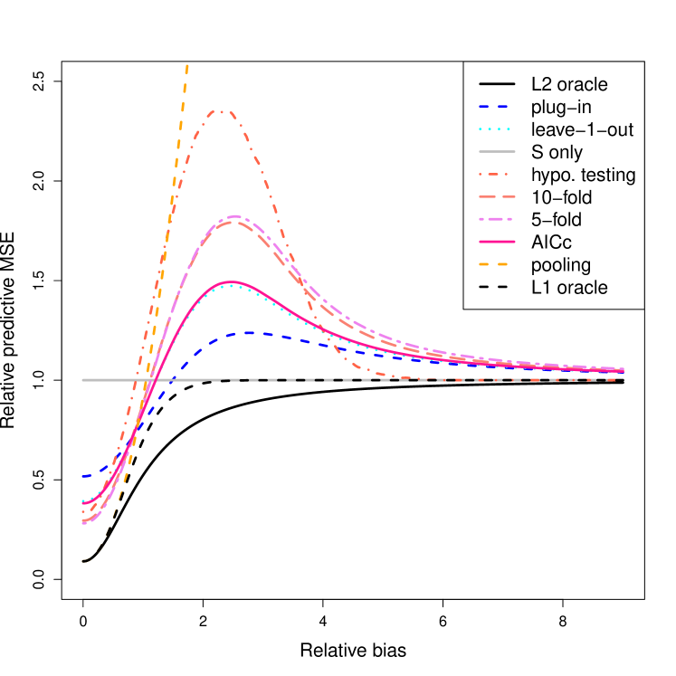
Figure 1: Numerical results for the location problem. The horizontal line at $1$ represents using the small sample only and ignoring the large one. The lowest line shown is for an oracle choosing $\lambda$ in the $L_{2}$ penalization. The dashed black curve shows an oracle using the $L_{1}$ penalization. The other curves are as described in the text.

The solid curve in Figure 1 shows the oracle’s value. It lies strictly below the horizontal $S$-only line. None of the competing curves lie strictly below that line. None can because $\bar{Y}_{S}$ is an admissible estimator for $d=1$ (Stein,, 1956). The second lowest curve in Figure 1 is for the oracle using the $L_{1}$ version of the penalty. The $L_{1}$ penalized oracle is not as effective as the $L_{2}$ oracle and it is also more difficult to approximate. The highest observed predictive MSEs come from a method of simply pooling the two samples. That method is very successful when the relative bias is near zero but has an MSE that becomes unbounded as the relative bias increases.

Now we discuss methods that use the data to decide whether to use the small sample only, pool the samples or choose an amount of shrinkage. We may list them in order of their worst case performance. From top (worst) to bottom (best) in Figure 1 they are: hypothesis testing, $5$-fold cross-validation, $10$-fold cross-validation, AICc, leave-one-out cross-validation, and then the simple plug-in method which is minimax among this set of choices. AICc and leave-one-out are very close. Our cross-validation estimators used $\omega=\max(\omega_{\mathrm{cv},K},n/(n+N))$ where $\omega_{\mathrm{cv},K}$ is given by (3.3).

The hypothesis testing method is based on a two-sample $t$-test of whether $\delta=0$. If the test is rejected at $\alpha=0.05$, then only the small sample data is used. If the test is not rejected, then the two samples are pooled. That test was based on $\sigma^{2}_{B}=\sigma^{2}_{S}$ which may give hypothesis testing a slight advantage in this setting (but it still performed poorly).

The AICc method performs virtually identically to leave-one-out cross-validation over the whole range of relative biases.

None of these methods makes any other one inadmissible: each pair of curves crosses. The methods that do best at large relative biases tend to do worst at relative bias near $0$ and vice versa. The exception is hypothesis testing. Compared to the others it does not benefit fully from low relative bias but it recovers the quickest as the bias increases. Of these methods hypothesis testing is best at the highest relative bias, $K$-fold cross-validation with small $K$ is best at the lowest relative bias, and the plug-in method is best in between.

Aggressive methods will do better at low bias but worse at high bias. What we see in this simulation is that $K$-fold cross-validation is the most aggressive followed by leave-one-out and AICc and that plug-in is least aggressive. These findings confirm what we saw in the formulas from Section 3. Hypothesis testing does not quite fit into this spectrum: its worst case performance is much worse than the most aggressive methods yet it fails to fully benefit from pooling when the bias is smallest. Unlike aggressive methods it does very well at high bias.

4.2 Regression

We simulated our data enrichment method for the following scenario. The small sample had $n=1000$ observations and the large sample had $N=10{,}000$. The true $\beta$ was taken to be $0$. This is no loss of generality because we are not shrinking $\beta$ towards $0$. The value of $\gamma$ was taken uniformly on the unit sphere in $d$ dimensions and then multiplied by a scale factor that we varied.

We considered $d=2,4,5$ and $10$. All of our examples included an intercept column of $1$s in both $X_{S}$ and $X_{B}$. The other $d-1$ predictors were sampled from a Gaussian distribution with covariance $C_{S}$ or $C_{B}$, respectively.

In one simulation we took $C_{S}$ and $C_{B}$ to be independent Wishart$(I,d-1,d-1)$ random matrices. In the other simulation, they were sampled as a spiked covariance model (Johnstone,, 2001). There $C_{S}=I_{d-1}+\rho uu^{\mathsf{T}}$ and $C_{B}=I_{d-1}+\rho vv^{\mathsf{T}}$ where $u$ and $v$ are independently and uniformly sampled from the unit sphere in $\mathbb{R}^{d-1}$ and $\rho\geq 0$ is a parameter that measures the lack of proportionality between covariances. We chose $\rho=d$ so that the sample specific portion of the variance has comparable magnitude to the common part.

The variance in the small sample was $\sigma^{2}_{S}=1$. To model the lower quality of the large sample we used $\sigma^{2}_{B}=2$.

We scaled the results so that regression using sample $S$ only yields a mean squared error of $1$. We computed the risk of an $L_{2}$ oracle, as well as sampling errors when $\lambda$ is estimated by the plug-in formula, by our bias-adjusted plug-in formula and via AICc. In addition we considered the simple weighted combination $\omega\hat{\beta}_{S}+(1-\omega)\hat{\beta}_{B}$ with $\omega$ chosen by the plug-in formula. To optimize (2.10) over $\lambda$ we used the optimize function in R which is based on golden section search (Brent,, 1973).

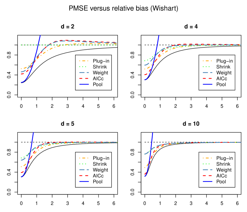
Figure 2: Predicted MSE versus relative bias for the Wishart covariances described in the text. On this scale the small sample only has MSE one (horizontal dashed line). Five methods are shown. The lowest curve is for the oracle.

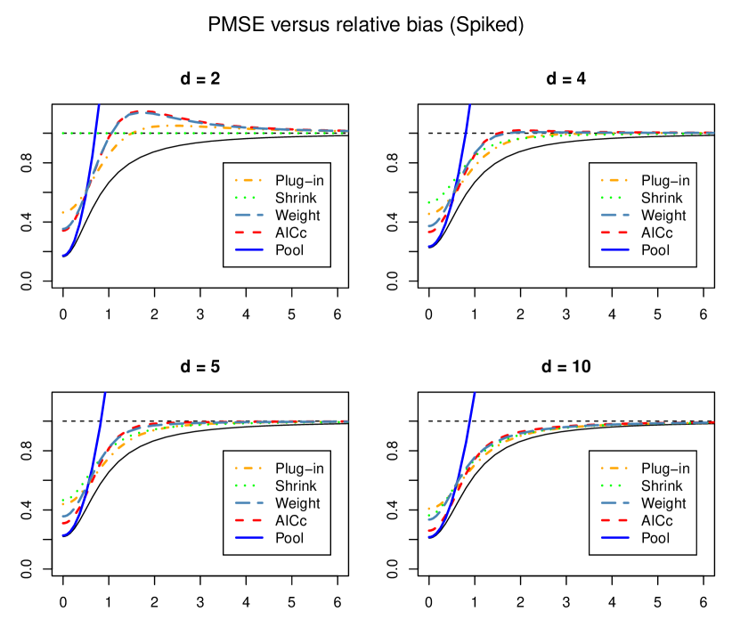
Figure 3: Predicted MSE versus relative bias for the spiked covariances described in the text. On this scale the small sample only has MSE one (horizontal dashed line). Five methods are shown. The lowest curve is for the oracle.

We also included a shrinkage estimator. Because our simulated runs all had $\beta_{S}=0$ it is not reasonable to include shrinkage of $\hat{\beta}_{S}$ towards zero in the comparison; we cannot in practice shrink towards the truth. Instead, we used the positive part Stein shrinkage estimate (2.13) shrinking $\hat{\beta}_{S}$ towards $\hat{\beta}_{B}$ but not past it. That shrinkage requires an estimate $\hat{\sigma}^{2}_{S}$ of $\sigma^{2}_{S}$. We used the true value, $\sigma^{2}_{S}=1$, giving the shrinkage estimator a slight advantage.

We did not include hypothesis testing in this example, because there are $2^{d}$ possible ways to decide which parameters to pool and which to estimate separately.

We simulated each of the two covariance models with each of the four dimensions $10{,}000$ times. For each method we averaged the squared prediction errors $(\hat{\beta}-\beta)^{\mathsf{T}}V_{S}(\hat{\beta}-\beta)$ and then divided those mean squared errors by the one for using the small sample only. Figures 2 and 3 show the results.

At small bias levels pooling the samples is almost as good as the oracle. But the loss for pooling samples grows without bound when the bias increases. For $d=2$, shrinkage amounts to using the small sample only but for $d>2$ it performs universally better than the small sample.

When comparing methods we see that the curves usually cross. Methods that are best at low bias tend not to be best at high bias. Note however that there is a lot to gain at low bias while the methods differ only a little at high bias. As a result the more aggressive methods making greater use of the large data are more likely to yield a big improvement.

The weighting estimator generally performs better than the shrinkage estimator in that it offers a meaningful improvement at low bias costing a minor relative loss at high bias. We analyze that estimator in Section 5. The plug-in estimator also is generally better than shrinkage. The AICc estimator is generally better than both of those. We do not show the bias adjusted plug-in estimators. Their performance is almost identical to AICc (always within about $0.015$). Of those, the one using $\widehat{\Theta}_{\mathrm{bapi}}$ was consistently at least as good as $\widetilde{\Theta}_{\mathrm{bapi}}$ and sometimes a little better.

The greatest gains are at or near zero bias. Table 1 shows the quadratic losses at $\delta=0$ normalized by the loss attained by the oracle. Pooling is almost as good as the oracle in this case but we rule it out because of its extreme bad performance when the bias is large. Some of our new estimators yield very much reduced squared error compared to the shrinkage estimator. For example three of the new methods’ squared errors are just less than half that of the shrinkage estimator for $d=10$ and the Wishart covariances.

Table 1: This table shows the quadratic loss (2.14) normalized by that of the oracle when $\delta=0$ (the no bias condition). The methods are described in the text.

	Wishart				Spiked
Method	2	4	5	10	2	4	5	10
Oracle	1.00	1.00	1.00	1.00	1.00	1.00	1.00	1.00
Pool	1.03	1.02	1.02	1.01	1.04	1.04	1.03	1.03
Small only	4.13	3.34	3.31	3.18	6.04	4.43	4.55	4.78
Shrink	4.13	2.29	2.27	2.42	6.04	2.35	2.12	1.74
Weighting	1.91	1.99	2.12	2.43	2.13	1.65	1.62	1.60
${\widetilde{\Theta}}_{\mathrm{plug}}$	2.17	1.73	1.69	1.56	2.80	2.01	2.00	1.95
${\widetilde{\Theta}}_{\mathrm{bapi}}$	1.77	1.39	1.33	1.19	2.13	1.52	1.47	1.31
${\widehat{\Theta}}_{\mathrm{bapi}}$	1.76	1.39	1.33	1.19	2.12	1.51	1.45	1.30
AICc	1.73	1.35	1.30	1.15	2.06	1.47	1.41	1.24

5 Inadmissibility

Section 4 gives empirical support for our proposal. Several of the estimators perform better than ordinary shrinkage. In this section we provide some theoretical support. We provide a data enriched estimator that makes least squares on the small sample inadmissible. The estimator is derived for the proportional design case but inadmissibility holds even when $V_{B}=X_{B}^{\mathsf{T}}X_{B}$ is not proportional to $V_{S}=X_{S}^{\mathsf{T}}X_{S}$. The inadmissibility is with respect to a loss function $\mathbb{E}(\|X_{T}(\hat{\beta}-\beta)\|^{2})$ where $V_{T}=X_{T}^{\mathsf{T}}X_{T}$ is proportional to $V_{S}$.

To motivate the estimator, suppose for the moment that $V_{B}=N\Sigma$, $V_{S}=n\Sigma$ and $V_{T}=\Sigma$ for a positive definite matrix $\Sigma$. Then the weighting matrix $W_{\lambda}$ in Lemma 2.1 simplifies to $W_{\lambda}=\omega I$ where $\omega=(N+n\lambda)/(N+n\lambda+N\lambda)$. As a result $\hat{\beta}=\omega\hat{\beta}_{S}+(1-\omega)\hat{\beta}_{B}$ and we can find and estimate an oracle’s value for $\omega$.

We show below that the resulting estimator of $\hat{\beta}$ with estimated $\omega$ dominates $\hat{\beta}_{S}$ (making it inadmissible) under mild conditions that do not require $V_{B}\propto V_{S}$. We do need the model degrees of freedom to be at least $5$, and it will suffice to have the error degrees of freedom in the small sample regression be at least $10$. The result also requires a Gaussian assumption in order to use a lemma of Stein’s.

Write $Y_{S}=X_{S}\beta+\varepsilon_{S}$ and $Y_{B}=X_{B}(\beta+\gamma)+\varepsilon_{B}$ for $\varepsilon_{S}\stackrel{{\scriptstyle\text{iid}}}{{\sim}}\mathcal{N}(0,\sigma_{S}^{2})$ and $\varepsilon_{B}\stackrel{{\scriptstyle\text{iid}}}{{\sim}}\mathcal{N}(0,\sigma_{B}^{2})$. The mean squared prediction error of $\omega\hat{\beta}_{S}+(1-\omega)\hat{\beta}_{B}$ is

$$f(\omega) =\mathbb{E}(\|X_{T}(\hat{\beta}(\omega)-\beta)\|^{2})$$

$$=\mathrm{tr}((\omega^{2}\sigma^{2}_{S}V_{S}^{-1}+(1-\omega)^{2}(\gamma\gamma^{\mathsf{T}}+\sigma^{2}_{B}V_{B}^{-1}))\Sigma).$$

This error is minimized by the oracle’s parameter value

$$\omega_{\mathrm{orcl}} =\frac{\mathrm{tr}((\gamma\gamma^{\mathsf{T}}+\sigma^{2}_{B}V_{B}^{-1})\Sigma)}{\mathrm{tr}((\gamma\gamma^{\mathsf{T}}+\sigma^{2}_{B}V_{B}^{-1})\Sigma)+\sigma_{S}^{2}\mathrm{tr}(V_{S}^{-1}\Sigma)}.$$

When $V_{S}=n\Sigma$ and $V_{B}=N\Sigma$, we find

$$\omega_{\mathrm{orcl}} =\frac{\gamma^{\mathsf{T}}\Sigma\gamma+d\sigma_{B}^{2}/N}{\gamma^{\mathsf{T}}\Sigma\gamma+d\sigma_{B}^{2}/N+d\sigma_{S}^{2}/n}.$$

The plug-in estimator is

$$\hat{\omega}_{\mathrm{plug}} =\frac{\hat{\gamma}^{\mathsf{T}}\Sigma\hat{\gamma}+d\hat{\sigma}_{B}^{2}/N}{\hat{\gamma}^{\mathsf{T}}\Sigma\hat{\gamma}+d\hat{\sigma}_{B}^{2}/N+d\hat{\sigma}_{S}^{2}/n}$$ (5.1)

where $\hat{\sigma}_{S}^{2}={\|Y_{S}-X_{S}\hat{\beta}_{S}\|^{2}}/{(n-d)}$ and $\hat{\sigma}_{B}^{2}={\|Y_{B}-X_{B}\hat{\beta}_{B}\|^{2}}/{(N-d)}$. To allow a later bias adjustment, we generalize this plug-in estimator. Let $h(\hat{\sigma}^{2}_{B})$ be any nonnegative measurable function of $\hat{\sigma}^{2}_{B}$ with $\mathbb{E}(h(\hat{\sigma}^{2}_{B}))<\infty$. The generalized plug-in estimator is

$$\hat{\omega}_{\mathrm{plug},h} =\frac{\hat{\gamma}^{\mathsf{T}}\Sigma\hat{\gamma}+h(\hat{\sigma}_{B}^{2})}{\hat{\gamma}^{\mathsf{T}}\Sigma\hat{\gamma}+h(\hat{\sigma}_{B}^{2})+d\hat{\sigma}_{S}^{2}/n}.$$ (5.2)

Here are the conditions under which $\hat{\beta}_{S}$ is made inadmissible by the data enrichment estimator.

Theorem 5.1.

Let $X_{S}\in\mathbb{R}^{n\times d}$ and $X_{B}\in\mathbb{R}^{N\times d}$ be fixed matrices with $X_{S}^{\mathsf{T}}X_{S}=n\Sigma$ and $X_{B}^{\mathsf{T}}X_{B}=V_{B}$ where $\Sigma$ and $V_{B}$ both have rank $d$. Let $Y_{S}\sim\mathcal{N}(X_{S}\beta,\sigma^{2}_{S}I_{n})$ independently of $Y_{B}\sim\mathcal{N}(X_{B}(\beta+\gamma),\sigma^{2}_{B}I_{N})$. If $d\geq 5$ and $m\equiv n-d\geq 10$, then

$$\mathbb{E}(\|X_{T}\hat{\beta}(\hat{\omega})-X_{T}\beta\|^{2}) <\mathbb{E}(\|X_{T}\hat{\beta}_{S}-X_{T}\beta\|^{2})$$ (5.3)

holds for any matrix $X_{T}$ with $X_{T}^{\mathsf{T}}X_{T}=\Sigma$ and any $\hat{\omega}=\hat{\omega}_{\mathrm{plug},h}$ given by (5.2).

Proof.

Section 9.7 in the Appendix. ∎

The condition on $m$ can be relaxed at the expense of a more complicated statement. From the details in the proof, it suffices to have $d\geq 5$ and $m(1-4/d)\geq 2$.

Because $\mathbb{E}(\hat{\gamma}^{\mathsf{T}}\Sigma\hat{\gamma})>\gamma^{\mathsf{T}}\Sigma\gamma$ we find that $\hat{\omega}_{\mathrm{plug}}$ is biased upwards, making it conservative. In the proportional design case we find that the bias is $d\sigma_{S}^{2}/n+d\sigma_{B}^{2}/N$. That motivates a bias adjustment, replacing $\hat{\gamma}^{\mathsf{T}}\Sigma\hat{\gamma}$ by $\hat{\gamma}^{\mathsf{T}}\Sigma\hat{\gamma}-d\hat{\sigma}^{2}_{S}/n-d\hat{\sigma}^{2}_{B}/N$. The result is

$$\hat{\omega}_{\mathrm{bapi}} =\frac{\hat{\gamma}^{\mathsf{T}}\Sigma\hat{\gamma}-d\hat{\sigma}_{S}^{2}/n}{\hat{\gamma}^{\mathsf{T}}\Sigma\hat{\gamma}}\vee\frac{n}{n+N},$$ (5.4)

where values below $n/(n+N)$ get rounded up. This bias-adjusted estimate of $\omega$ is not covered by Theorem 5.1. Subtracting only $\hat{\sigma}^{2}_{B}/N$ instead of $\hat{\sigma}^{2}_{B}/N+\hat{\sigma}^{2}_{S}/n$ is covered, yielding

$$\hat{\omega}_{\mathrm{bapi}}^{\prime} =\frac{\hat{\gamma}^{\mathsf{T}}\Sigma\hat{\gamma}}{\hat{\gamma}^{\mathsf{T}}\Sigma\hat{\gamma}+d\hat{\sigma}_{S}^{2}/n},$$ (5.5)

which corresponds to taking $h(\hat{\sigma}^{2}_{B})\equiv 0$ in equation (5.2). Data enrichment with $\hat{\omega}$ given by (5.4) makes $\hat{\beta}_{S}$ inadmissible whether or not the motivating covariance proportionality holds.

6 A matrix oracle

In this section we look for an explanation of how data enrichment might be more accurate than Stein shrinkage. We generalize our estimator to

$$\hat{\beta}(W)=W\hat{\beta}_{S}+(I-W)\hat{\beta}_{B}$$

and then find the optimal matrix $W$.

Theorem 6.1.

Let $\hat{\beta}_{S}\in\mathbb{R}^{d}$ have mean $\beta$ and covariance matrix $\sigma^{2}_{S}V_{S}^{-1}$ for $\sigma_{S}>0$. Let $\hat{\beta}_{B}\in\mathbb{R}^{d}$ be independent of $\hat{\beta}_{S}$, with mean $\beta+\gamma$ and covariance matrix $\sigma^{2}_{B}V_{B}^{-1}$ for $\sigma_{B}>0$. Let $\hat{\beta}(W)=W\hat{\beta}_{S}+(I-W)\hat{\beta}_{B}$ for a matrix $W\in\mathbb{R}^{d\times d}$. Let $V_{T}\in\mathbb{R}^{d\times d}$ be any positive definite symmetric matrix. Then $\mathbb{E}((\hat{\beta}(W)-\beta)^{\mathsf{T}}V_{T}(\hat{\beta}(W)-\beta))$ is minimized at

$$W=(\gamma\gamma^{\mathsf{T}}+\sigma^{2}_{B}V_{B}^{-1}+\sigma^{2}_{S}V_{S}^{-1})^{-1}(\gamma\gamma^{\mathsf{T}}+\sigma^{2}_{B}V_{B}^{-1}).$$ (6.1)

Proof.

Section 9.8. ∎

It is interesting that when we are free to choose the entire $d\times d$ matrix $W$, then the optimal choice is the same for all weighting matrices $V_{T}$.

The penalized least squares criterion (2.1) leads to a matrix weighting of the two within-sample estimators. The weighting matrix $W_{\lambda}$ is in a one dimensional family indexed by $0\leq\lambda\leq\infty$. The optimal $W$ from (6.1) is not generally in that family.

Both $W_{\lambda}$ from criterion (2.1) and $W$ from (6.1) trade off bias and variance, through the appearance $\gamma\gamma^{\mathsf{T}}$, $\sigma^{2}_{S}$, and $\sigma^{2}_{B}$, which for (2.1) appear in the formula for the optimal $\lambda$. The advantage of working with $W_{\lambda}$ instead of $W$ is that $W_{\lambda}$ yields a one parameter family of candidate weighting matrices to search over.

When $V_{S}$ and $V_{B}$ are both proportional to the same positive definite matrix $V_{T}$, then the data enrichment oracle chooses $W=\omega I_{d}$ where

$$\omega=\omega_{\mathrm{orcl}}=\frac{\mathrm{tr}((\gamma\gamma^{\mathsf{T}}+\sigma^{2}_{B}V_{B}^{-1})V_{T})}{\mathrm{tr}([\gamma\gamma^{\mathsf{T}}+\sigma^{2}_{B}V_{B}^{-1}+\sigma_{S}^{2}V_{S}^{-1}]V_{T})}$$

which mimicks the form of the optimal $W$ in equation (6.1), replacing numerator and denominator by traces after multiplying both by $V_{T}$.

The James-Stein shrinker chooses $W=\omega_{\mathrm{JS}}I_{d}$ where

$$\omega_{\mathrm{JS}}=1-\frac{d-2}{\|\hat{\theta}_{S}-\hat{\theta}_{B}\|^{2}/\sigma^{2}_{S}}=1-\frac{d-2}{\hat{\gamma}^{\mathsf{T}}V_{S}\hat{\gamma}/\sigma^{2}_{S}}.$$

If we approximate $\hat{\gamma}^{\mathsf{T}}V_{S}\hat{\gamma}$ by its expectation $\mathrm{tr}((\gamma\gamma^{\mathsf{T}}+\sigma^{2}_{S}V_{S}^{-1}+\sigma^{2}_{B}V_{B}^{-1})V_{S})$ we find $\omega_{\mathrm{JS}}$ centered around

$$\widetilde{\omega}_{\mathrm{JS}}=\frac{\mathrm{tr}((\gamma\gamma^{\mathsf{T}}+\sigma^{2}_{B}V_{B}^{-1})V_{S})+2\sigma^{2}_{S}}{\mathrm{tr}((\gamma\gamma^{\mathsf{T}}+\sigma^{2}_{B}V_{B}^{-1}+\sigma^{2}_{S}V_{S}^{-1})V_{S})}.$$

The presence of $2\sigma^{2}_{S}$ in the numerator leads the James-Stein approach to make less aggressive use of the big data set than data enrichment does. We believe that this is why the James-Stein method did not perform well in our simulations.

7 Related literatures

There are many disjoint literatures that study problems like the one we have presented. They do not seem to have been compared before, the literatures seem to be mostly unaware of each other, and there is a surprisingly large variety of problem contexts. Some quite similar sounding problems turn out to differ on critically important details. We give a brief summary of those topics here.

The key ingredient in our problem is that we care more about the small sample than the large one. Were that not the case, we could simply pool all the data and fit a model with indicator variables picking out one or indeed many different special subsets of interest. Without some kind of regularization, that approach ends up being similar to taking $\lambda=0$ and hence does not borrow strength.

The closest match to our problem setting comes from small area estimation in survey sampling. The monograph by Rao, (2003) is a comprehensive treatment of that work and Ghosh and Rao, (1994) provide a compact summary. In that context the large sample may be census data from the entire country and the small sample (called the small area) may be a single county or a demographically defined subset. Every county or demographic group may be taken to be the small sample in its turn. The composite estimator (Rao,, 2003, Chapter 4.3) is a weighted sum of estimators from small and large samples. The estimates being combined may be more complicated than regressions, involving for example ratio estimates. The emphasis is usually on scalar quantities such as small area means or totals, instead of the regression coefficients we consider. One particularly useful model (Ghosh and Rao,, 1994, equation (4.2)) allows the small areas to share regression coefficients apart from an area specific intercept. Then BLUP estimation methods lead to shrinkage estimators similar to ours.

Our methods and results are similar to empirical Bayes methods, drawing heavily on ideas of Charles Stein. A Stein-like result also holds for multiple regression in the context of just one sample. We mentioned already the regression shrinkers of Copas, (1983) and Stein, (1960). Efron and Morris, 1973a find that the Stein effect for shrinking to a common mean takes place at dimension $4$ and George, (1986) finds that the effect takes place at dimension $3+q$ when shrinking means towards a $q$–dimensional linear manifold.

A similar problem to ours is addressed by Chen and Chen, (2000). Like us, they have $(X,Y)$ pairs of both high and low quality. In their setting both high and low quality pairs are defined for the same set of individuals. Their given sample has all of the low quality data and the high quality data are available only on a simple random sample of the subjects.

Boonstra et al., 2013a consider a genomics problem where there are both low and high quality versions of $X$, from two different technical platforms, but all data share the same $Y$. All observations have the low quality $X$’s while a subset have both high and low quality $X$ measurements. They take a Bayesian approach. Boonstra et al., 2013b handle the same problem via shrinkage estimates. A crucial difference in our setting, is that the subjects are completely different in our two samples; no $(X,Y)$ pair in one data set comes from the same person as an $(X,Y)$ pair in the other data set.

Mukherjee and Chatterjee, (2008) use shrinkage methods to blend two estimators. One is a case-control estimate of a log odds ratio. The other is a case-only estimator, derived under an assumption of gene-environment independence. They also derive and employ a plug-in estimator. Their target parameter is scalar so no Stein effect could be expected. Chen et al., (2009) address the same issue via $L_{1}$ and $L_{2}$ shrinkage based methods, and give some asymptotic covariances.

In chemometrics, a calibration transfer problem (Feudale et al.,, 2002) comes up when one wants to adjust a model to new spectral hardware. There may be a regression model linking near-infrared spectroscopy data to a property of some sample material. The transfer problem comes up for data from a new machine. Sometimes one can simply run a selection of samples through both machines but in other cases that is not possible, perhaps because one machine is remote (Woody et al.,, 2004). Their primary and secondary instruments correspond to our small and big samples respectively. Their emphasis is on transfering either principal components regression or partial least squares models, not the plain regressions we consider here.

A common problem in marketing is data fusion, also known as statistical matching. Variables $(X,Y)$ are measured in one sample while variables $(X,Z)$ are measured in another. There may or may not be a third sample with some measured triples $(X,Y,Z)$. The goal in data fusion is to use all of the data to form a large synthetic data set of $(X,Y,Z)$ values, perhaps by imputing missing $Z$ for the $(X,Y)$ sample and/or missing $Y$ for the $(X,Z)$ sample. When there is no $(X,Y,Z)$ sample, some untestable assumptions must be made about the joint distribution, because it cannot be recovered from its bivariate margins. The text by D’Orazio et al., (2006) gives a comprehensive summary of what can and cannot be done. Many of the approaches are based on methods for handling missing data (Little and Rubin,, 2009).

Medicine and epidemiology among other fields use meta-analysis (Borenstein et al.,, 2009). In that setting there are $(X,Y)$ data sets from numerous environments, no one of which is necessarily of primary importance.

Our problem is an instance of what machine learning researchers call domain adaptation. They may have fit a model to a large data set (the ‘source’) and then wish to adapt that model to a smaller specialized data set (the ‘target’). This is especially common in natural language processing. NIPS 2011 included a special session on domain adaptation. In their motivating problems there are typically a very large number of features (e.g., one per unique word appearing in a set of documents). They also pay special attention to problems where many of the data points do not have a measured response. Quite often a computer can gather high dimensional $X$ while a human rater is necessary to produce $Y$. Daumé, (2009) surveys various wrapper strategies, such as fitting a model to weighted combinations of the data sets, deriving features from the reference data set to use in the target one and so on. Cortes and Mohri, (2011) consider domain adaptation for kernel-based regularization algorithms, including kernel ridge regression, support vector machines (SVMs), or support vector regression (SVR). They prove pointwise loss guarantees depending on the discrepancy distance between the empirical source and target distributions, and demonstrate the power of the approach on a number of experiments using kernel ridge regression. We have given conditions under which adaptation is always beneficial.

A related term in machine learning is concept drift (Widmer and Kubat,, 1996). There a prediction method may become out of date as time goes on. The term drift suggests that slow continual changes are anticipated, but they also consider that there may be hidden contexts (latent variables in statistical teminology) affecting some of the data.

8 Conclusions

We have studied a middle ground between pooling a large data set into a smaller target one and ignoring it completely. Looking at the left side of Figures 1, 2 and 3 we see that in the low bias cases the more aggressive methods have a clear advantage. Fortune favors the bold. Pooling is the boldest and wins the most when bias is small. But pooling has unbounded risk as bias increases. That is, misfortune also favors the bold. Our shrinkage methods provide a compromise. In higher dimensional settings of Figures 2 and 3, we see that AICc and bias adjusted plug-in gain a lot of efficiency when the bias is low. When the bias is high, they are squeezed into a narrow band between the oracle performance and that of $\hat{\beta}_{S}$ which ignores the big data set. As a result, the new methods show large improvements compared to shrinkage when the bias small but only lose a little when the bias is large.

9 Appendix I: proofs

This appendix presents proofs of the results in this article. They are grouped into sections by topic, with some technical supporting lemmas separated into their own sections.

9.1 Proof of Theorem 2.1

Proof.

First

$$\mathrm{df}(\lambda)=\sigma^{-2}_{S}\mathrm{tr}(\mathrm{cov}(X_{S}\hat{\beta},Y_{S}))=\sigma^{-2}_{S}\mathrm{tr}(X_{S}W_{\lambda}(X_{S}^{\mathsf{T}}X_{S})^{-1}X_{S}^{\mathsf{T}}\sigma^{2}_{S})=\mathrm{tr}(W_{\lambda}).$$

Next with $X_{T}=X_{S}$, and $M=V_{S}^{1/2}V_{B}^{-1}V_{S}^{1/2}$,

$$\mathrm{tr}(W_{\lambda})=\mathrm{tr}(V_{S}+\lambda V_{S}V_{B}^{-1}V_{S}+\lambda V_{S})^{-1}(V_{S}+\lambda V_{S}V_{B}^{-1}V_{S}).$$

We place $V_{S}^{1/2}V_{S}^{-1/2}$ between these factors and absorb them left and right. Then we reverse the order of the factors and repeat the process, yielding

$$\mathrm{tr}(W_{\lambda})=\mathrm{tr}(I+\lambda M+\lambda I)^{-1}(I+\lambda M).$$

Writing $M=U\mathrm{diag}(\nu_{1},\dots,\nu_{d})U^{\mathsf{T}}$ for an orthogonal matrix $U$ and simplifying yields the result. ∎

9.2 Proof of Theorem 2.2

Proof.

First $\mathbb{E}(\|X_{T}\hat{\beta}-X_{T}\beta\|^{2})=\mathrm{tr}(V_{S}\mathbb{E}((\hat{\beta}-\beta)(\hat{\beta}-\beta)^{\mathsf{T}}))$. Next using $W=W_{\lambda}$, we make a bias-variance decomposition,

$$\mathbb{E}\bigl{(}(\hat{\beta}-\beta)(\hat{\beta}-\beta)^{\mathsf{T}}\bigr{)} =(I-W)\gamma\gamma^{\mathsf{T}}(I-W)^{\mathsf{T}}+\mathrm{cov}(W\hat{\beta}_{S})+\mathrm{cov}((I-W)\hat{\beta}_{B})$$

$$=\sigma_{S}^{2}WV_{S}^{-1}W^{\mathsf{T}}+(I-W)\Theta(I-W)^{\mathsf{T}},$$

for $\Theta=\gamma\gamma^{\mathsf{T}}+\sigma^{2}_{B}V_{B}^{-1}$. Therefore $\mathbb{E}\bigl{(}\|X_{S}(\hat{\beta}-\beta)\|^{2}\bigr{)}=\sigma_{S}^{2}\mathrm{tr}(V_{S}WV_{S}^{-1}W^{\mathsf{T}})+\mathrm{tr}(\Theta(I-W)^{\mathsf{T}}V_{S}(I-W)).$

Now we introduce $\widetilde{W}=V_{S}^{1/2}WV_{S}^{-1/2}$ finding

$$\widetilde{W} =V_{S}^{1/2}(V_{B}+\lambda V_{S}+\lambda V_{B})^{-1}(V_{B}+\lambda V_{S})V_{S}^{-1/2}$$

$$=(I+\lambda M+\lambda I)^{-1}(I+\lambda M)$$

$$=U\widetilde{D}U^{\mathsf{T}},$$

where $\widetilde{D}=\mathrm{diag}((1+\lambda\nu_{j})/(1+\lambda+\lambda\nu_{j}))$. This allows us to write the first term of the mean squared error as

$$\sigma^{2}_{S}\mathrm{tr}(V_{S}WV_{S}^{-1}W^{\mathsf{T}})=\sigma^{2}_{S}\mathrm{tr}(\widetilde{W}\widetilde{W}^{\mathsf{T}})=\sigma^{2}_{S}\sum_{j=1}^{d}\frac{(1+\lambda\nu_{j})^{2}}{(1+\lambda+\lambda v_{j})^{2}}.$$

For the second term, let $\widetilde{\Theta}=V_{S}^{1/2}\Theta V_{S}^{1/2}$. Then

$$\mathrm{tr}\bigl{(}\Theta(I-W)^{\mathsf{T}}V_{S}(I-W)\bigr{)} =\mathrm{tr}(\widetilde{\Theta}(I-\widetilde{W})^{\mathsf{T}}(I-\widetilde{W}))$$

$$=\mathrm{tr}(\tilde{\Theta}U(I-\widetilde{D})^{2}U^{\mathsf{T}})$$

$$=\lambda^{2}\sum_{k=1}^{d}\frac{u_{k}^{\mathsf{T}}V_{S}^{1/2}\Theta V_{S}^{1/2}u_{k}}{(1+\lambda+\lambda\nu_{k})^{2}}.\ \qed$$

9.3 Derivation of equation (3.3)

We suppose for simplicity that $n=rK$ for an integer $r$, so the $K$ folds have equal size. In that case $\bar{Y}_{S,-k}=(n\bar{Y}_{S}-r\bar{Y}_{S,k})/(n-r)$. Now

$$\omega_{\mathrm{cv}} =\frac{\sum_{k}(\bar{Y}_{S,-k}-\bar{Y}_{B})(\bar{Y}_{S,k}-\bar{Y}_{B})}{\sum_{k}(\bar{Y}_{S,-k}-\bar{Y}_{B})^{2}}$$ (9.1)

After some algebra, the numerator of (9.1) is

$$K(\bar{Y}_{S}-\bar{Y}_{B})^{2}-\frac{r}{n-r}\sum_{k=1}^{K}(\bar{Y}_{S,k}-\bar{Y}_{S})^{2}$$

and the denominator is

$$K(\bar{Y}_{S}-\bar{Y}_{B})^{2}+\biggl{(}\frac{r}{n-r}\biggr{)}^{2}\sum_{k=1}^{K}(\bar{Y}_{S,k}-\bar{Y}_{S})^{2}.$$

Letting $\hat{\delta}_{0}=\bar{Y}_{B}-\bar{Y}_{S}$ and $\hat{\sigma}^{2}_{S,K}=(1/K)\sum_{k=1}^{K}(\bar{Y}_{S,k}-\bar{Y}_{S})^{2}$, we have

$$\omega_{\mathrm{cv}}=\frac{\hat{\delta}_{0}^{2}-\hat{\sigma}^{2}_{S,K}/(K-1)}{\hat{\delta}_{0}^{2}+\hat{\sigma}^{2}_{S,K}/(K-1)^{2}}.$$

The only quantity in $\omega_{\mathrm{cv}}$ which depends on the specific $K$-way partition used is $\hat{\sigma}^{2}_{S,K}$. If the groupings are chosen by sampling without replacement, then under this sampling,

$$\mathbb{E}(\hat{\sigma}^{2}_{S,K})=\mathbb{E}((\bar{Y}_{S,1}-\bar{Y}_{S})^{2})=\frac{s^{2}_{S}}{r}(1-1/K)$$

using the finite population correction for simple random sampling, where $s^{2}_{S}=\hat{\sigma}^{2}_{S}n/(n-1)$. This simplifies to

$$\mathbb{E}(\hat{\sigma}^{2}_{S,K})=\hat{\sigma}^{2}_{S}\frac{n}{n-1}\frac{1}{r}\frac{K-1}{K}=\hat{\sigma}^{2}_{S}\frac{K-1}{n-1}.$$

Replacing $\hat{\sigma}^{2}_{S,K}$ in $\omega_{\mathrm{cv}}$ by its expectation yields (3.3).

9.4 Proof of Theorem 3.1

Proof.

If $\lambda>nN|\bar{Y}_{B}-\bar{Y}_{S}|/(n+N)$ then we may find directly that with any value of $\delta>0$ and corresponding $\mu$ given by (3.5), the derivative of (3.4) with respect to $\delta$ is positive. Therefore $\hat{\delta}\leq 0$ and a similar argument gives $\hat{\delta}\geq 0$, so that $\hat{\delta}=0$ and then $\hat{\mu}=(n\bar{Y}_{S}+N\bar{Y}_{B})/(n+N)$.

Now suppose that $\lambda\leq\lambda_{*}$. We verify that the quantities in (3.6) jointly satisfy equations (3.5). Substituting $\hat{\delta}$ from (3.6) into the first line of (3.5) yields

$$\frac{n\bar{Y}_{S}+N(\bar{Y}_{S}+\lambda(N+n)\eta/(Nn))}{n+N}=\bar{Y}_{S}+\frac{\lambda}{n}\mathrm{sign}(\bar{Y}_{B}-\bar{Y}_{S}),$$

matching the value in (3.6). Conversely, substituting $\hat{\mu}$ from (3.6) into the second line of (3.5) yields

$$\Theta\Bigl{(}\bar{Y}_{B}-\hat{\mu};\frac{\lambda}{N}\Bigr{)} =\Theta\Bigl{(}\bar{Y}_{B}-\bar{Y}_{S}-\frac{\lambda}{n}\mathrm{sign}(\bar{Y}_{B}-\bar{Y}_{S});\frac{\lambda}{N}\Bigr{)}.$$ (9.2)

Because of the upper bound on $\lambda$, the result is $\bar{Y}_{B}-\bar{Y}_{S}-\lambda(1/n+1/N)\mathrm{sign}(\bar{Y}_{B}-\bar{Y}_{S})$ which matches the value in (3.6). ∎

9.5 Derivation of equation (3.7)

Let $f=n/(n+N)$ be the fraction of the pooled data coming from the small sample and $F=1-f$ be the fraction from the large sample. Define $D=\bar{Y}_{B}-\bar{Y}_{S}$ and $c=\lambda/(nF)=\lambda(1/n+1/N)$. Then

$$\hat{\mu} =\begin{cases}\bar{Y}_{S}+{\lambda}/n\,\mathrm{sign}(D),&|D|\geq c\\ f\bar{Y}_{S}+F\bar{Y}_{B},&|D|\leq c\end{cases}$$

$$=F\bar{Y}_{B}+f\bar{Y}_{S}+((\lambda/n)\mathrm{sign}(D)-FD)1_{|D|\geq c}.$$

We replace $\bar{Y}_{B}$ and $\bar{Y}_{S}$ by linear combinations of $D$ and another variable $H$ chosen to be statistically independent of $D$. Specifically, $H=\bar{Y}_{B}+\alpha\bar{Y}_{S}$ for $\alpha=(\sigma^{2}_{B}/N)/(\sigma^{2}_{S}/n)$. The inverse transformation is

$$\begin{pmatrix}\bar{Y}_{S}\\ \bar{Y}_{B}\end{pmatrix}=\frac{1}{\alpha+1}\begin{pmatrix}-1&1\\ \alpha&1\\ \end{pmatrix}\begin{pmatrix}D\\ H\end{pmatrix}.$$

In terms of these independent variables we have

$$\hat{\mu}=c_{0}D+c_{1}H+((\lambda/n)\mathrm{sign}(D)-FD)1_{|D|\geq c}$$

where $c_{0}=\alpha/(\alpha+1)-f$, and $c_{1}=1/(\alpha+1)$.

Without loss of generality, $\mu=0$. Then $D\sim\mathcal{N}(\delta,\sigma^{2}_{S}/n+\sigma^{2}_{B}/N)$ independently of $H\sim\mathcal{N}(\delta,\alpha^{2}\sigma^{2}_{S}/n+\sigma^{2}_{B}/N)$. After some algebra,

$$\begin{split}\mathbb{E}(\hat{\mu}-\mu)^{2}&=c_{0}^{2}\mathbb{E}(D^{2})+c_{1}^{2}\mathbb{E}(H^{2})+2c_{0}c_{1}\mathbb{E}(D)\mathbb{E}(H)\\ &\quad+(\lambda/n)^{2}\mathbb{E}(1_{|D|\geq c})-2c_{1}F\mathbb{E}(H)\mathbb{E}\bigl{(}D1_{|D|\geq c}\bigr{)}\\ &\quad+F(F-2c_{0})\mathbb{E}\bigl{(}D^{2}1_{|D|\geq c}\bigr{)}\\ &\quad+2c_{1}(\lambda/n)\mathbb{E}(H)\mathbb{E}\bigl{(}\mathrm{sign}(D)1_{|D|\geq c}\bigr{)}\\ &\quad+2(\lambda/n)(c_{0}-F)\mathbb{E}\bigl{(}D\,\mathrm{sign}(D)1_{|D|\geq c}\bigr{)}.\end{split}$$ (9.3)

In addition to first and second moments of $D$ and $H$, we need some expectations of functions of $D$ involving the sign function and some indicators. They are given by Lemma 9.1 below. Let $\varphi$ and $\Phi$ be the probabilty density and cumulative distribution functions respectively of the $\mathcal{N}(0,1)$ distribution.

Lemma 9.1.

Let $D\sim\mathcal{N}(\delta,\tau^{2})$. Define $\eta_{+}=(\delta-c)/\tau$, $\eta_{-}=(-\delta-c)/\tau$, $\Phi_{\pm}=\Phi(\eta_{\pm})$ and $\varphi_{\pm}=\varphi(\eta_{\pm})$. Then for $c\geq 0$,

$$\mathbb{E}(1_{|D|\geq c}) =\Phi_{+}+\Phi_{-}$$ (9.4)

$$\mathbb{E}(D1_{|D|\geq c}) =\delta(\Phi_{+}+\Phi_{-})+\tau(\varphi_{+}-\varphi_{-})$$ (9.5)

$$\mathbb{E}(D^{2}1_{|D|\geq c}) =(\delta^{2}+\tau^{2})(\Phi_{+}+\Phi_{-})$$ (9.6)

$$\quad+\tau c(\varphi_{+}+\varphi_{-})+\tau\delta(\varphi_{+}-\varphi_{-})$$

$$\mathbb{E}(\mathrm{sign}(D)1_{|D|\geq c}) =\Phi_{+}-\Phi_{-},\quad\text{and}$$ (9.7)

$$\mathbb{E}(D\,\mathrm{sign}(D)1_{|D|\geq c}) =\delta(\Phi_{+}-\Phi_{-})+\tau(\varphi_{+}+\varphi_{-}).$$ (9.8)

Proof.

Equation (9.4) is almost immediate. For $Z\sim\mathcal{N}(0,1)$, using Chapter 2.5.1 of Patel and Read, (1996) yields $\mathbb{E}(Z1_{Z\leq c})=g_{1}(c)\equiv-\varphi(c)$ and $\mathbb{E}(Z^{2}1_{Z\leq c})=g_{2}(c)\equiv\Phi(c)-c\varphi(c)$. For $D\sim\mathcal{N}(\delta,\tau^{2})$ we may write $D=\delta+\tau Z$ and then

$$\mathbb{E}(D1_{D\leq c}) =g_{1}(c,\delta,\tau)\equiv\delta\Phi\Bigl{(}\frac{c-\delta}{\tau}\Bigr{)}+\tau g_{1}\Bigl{(}\frac{c-\delta}{\tau}\Bigr{)}$$

$$=\delta\Phi\Bigl{(}\frac{c-\delta}{\tau}\Bigr{)}-\tau\varphi\Bigl{(}\frac{c-\delta}{\tau}\Bigr{)},\quad\text{and}$$

$$\mathbb{E}(D^{2}1_{D\leq c}) =g_{2}(c,\delta,\tau)\equiv\delta^{2}\Phi\Bigl{(}\frac{c-\delta}{\tau}\Bigr{)}+2\delta\tau g_{1}\Bigl{(}\frac{c-\delta}{\tau}\Bigr{)}+\tau^{2}g_{2}\Bigl{(}\frac{c-\delta}{\tau}\Bigr{)}$$

$$=(\delta^{2}+\tau^{2})\Phi\Bigl{(}\frac{c-\delta}{\tau}\Bigr{)}-\tau(c+\delta)\varphi\Bigl{(}\frac{c-\delta}{\tau}\Bigr{)}.$$

For $c>0$, we write $1_{|D|\geq c}=1_{D\leq-c}+1_{D\geq c}=1_{D\leq-c}+1_{-D\leq-c}$, and so $\mathbb{E}(D1_{|D|\geq c})=g_{1}(-c,\delta,\tau)-g_{1}(-c,-\delta,\tau)$ which simplifies to (9.5). Similarly $\mathbb{E}(D^{2}1_{|D|\geq c})=g_{2}(-c,\delta,\tau)+g_{2}(-c,-\delta,\tau)$ which simplifies to (9.6).

Equation (9.7) follows upon writing $1_{|D|\geq c}=1_{D\geq c}-1_{-D\geq c}$. For (9.8) that step yields $\mathbb{E}(D\,\mathrm{sign}(D)1_{|D|\geq c})=g_{1}(-c,-\delta,\tau)-g_{1}(-c,\delta,\tau)$ ∎

The formula in the article follows by making substitutions of the quantities from Lemma 9.1 into equation (9.3). It also uses the identity $c_{0}+c_{1}=F$.

9.6 Supporting lemmas for inadmissibility

In this section we first recall Stein’s Lemma. Then we prove two technical lemmas used in the proof of Theorem 5.1.

Lemma 9.2.

Let $Z\sim\mathcal{N}(0,1)$ and let $g:\mathbb{R}\to\mathbb{R}$ be an indefinite integral of the Lebesgue measurable function $g^{\prime}$, essentially the derivative of $g$. If $\mathbb{E}(|g^{\prime}(Z)|)<\infty$ then

$$\mathbb{E}(g^{\prime}(Z))=\mathbb{E}(Zg(Z)).$$

Proof.

Stein, (1981). ∎

Lemma 9.3.

Let $\eta\sim\mathcal{N}(0,I_{d})$, $b\in\mathbb{R}^{d}$, and let $A>0$ and $B>0$ be constants. Let

$$Z=\eta+\frac{A(b-\eta)}{\|b-\eta\|^{2}+B}.$$

Then

$$\mathbb{E}(\|Z\|^{2}) <d+\mathbb{E}\left(\frac{A(A+4-2d)}{\|b-\eta\|^{2}+B}\right).$$

Proof.

First,

$$\mathbb{E}(\|Z\|^{2}) =d+\mathbb{E}\left(\frac{A^{2}\|b-\eta\|^{2}}{(\|b-\eta\|^{2}+B)^{2}}\right)+2A\sum_{k=1}^{d}\mathbb{E}\left(\frac{\eta_{k}(b_{k}-\eta_{k})}{\|b-\eta\|^{2}+B}\right).$$

Now define

$$g(\eta_{k})=\frac{b_{k}-\eta_{k}}{\|b-\eta\|^{2}+B}=\frac{b_{k}-\eta_{k}}{(b_{k}-\eta_{k})^{2}+\|b_{-k}-\eta_{-k}\|^{2}+B}.$$

By Stein’s lemma (Lemma 9.2), we have

$$\mathbb{E}\left(\frac{\eta_{k}(b_{k}-\eta_{k})}{\|b-\eta\|^{2}+B}\right) =\mathbb{E}(g^{\prime}(\eta_{k}))=\mathbb{E}\left(\frac{2(b_{k}-\eta_{k})^{2}}{(\|b-\eta\|^{2}+B)^{2}}-\frac{1}{\|b-\eta\|^{2}+B}\right)$$

and thus

$$\mathbb{E}(\|Z\|^{2}) =d+\mathbb{E}\left(\frac{(4A+A^{2})\|b-\eta\|^{2}}{(\|b-\eta\|^{2}+B)^{2}}-\frac{2Ad}{\|b-\eta\|^{2}+B}\right)$$

$$=d+\mathbb{E}\left(\frac{(4A+A^{2}-2Ad)}{\|b-\eta\|^{2}+B}-\frac{(4A+A^{2})B}{(\|b-\eta\|^{2}+B)^{2}}\right),$$

after collecting terms. ∎

Lemma 9.4.

For integer $m\geq 1$, let $Q\sim\chi_{(m)}^{2}$, $C>1$, $D>0$ and put

$$Z=\frac{Q(C-m^{-1}Q)}{Q+D}.$$

Then

$$\mathbb{E}(Z) \geq\frac{(C-1)m-2}{m+2+D}.$$

and so $\mathbb{E}(Z)>0$ whenever $C>1+{2}/{m}$.

Proof.

The $\chi^{2}_{(m)}$ density function is $p_{m}(x)=({2^{m/2-1}\Gamma(\frac{m}{2})})^{-1}x^{m/2-1}e^{-x/2}$. Thus

$$\mathbb{E}(Z) =\frac{1}{2^{m/2}\Gamma(\frac{m}{2})}\int_{0}^{\infty}\frac{x(C-m^{-1}x)}{x+D}x^{m/2-1}e^{-x/2}\,\mathrm{d}x$$

$$=m\int_{0}^{\infty}\frac{C-m^{-1}x}{x+D}p_{m+2}(x)\,\mathrm{d}x$$

$$\geq m\frac{C-(m+2)/m}{m+2+D}$$

by Jensen’s inequality. ∎

9.7 Proof of Theorem 5.1

We prove this first for $\hat{\omega}_{\mathrm{plug},h}=\hat{\omega}_{\mathrm{plug}}$, that is, taking $h(\hat{\sigma}^{2}_{B})=d\hat{\sigma}^{2}_{B}/n$. We also assume at first that $V_{B}=N\Sigma$ but remove the assumption later.

Note that $\hat{\beta}_{S}=\beta+(X_{S}^{\mathsf{T}}X_{S})^{-1}X_{S}^{\mathsf{T}}\varepsilon_{S}$ and $\hat{\beta}_{B}=\beta+\gamma+(X_{B}^{\mathsf{T}}X_{B})^{-1}X_{B}^{\mathsf{T}}\varepsilon_{B}$. It is convenient to define

$$\eta_{S} =\Sigma^{1/2}(X_{S}^{\mathsf{T}}X_{S})^{-1}X_{S}^{\mathsf{T}}\varepsilon_{S}\quad\text{and}\quad\eta_{B}=\Sigma^{1/2}(X_{B}^{\mathsf{T}}X_{B})^{-1}X_{B}^{\mathsf{T}}\varepsilon_{B}.$$

Then we can rewrite $\hat{\beta}_{S}=\beta+\Sigma^{-1/2}\eta_{S}$ and $\hat{\beta}_{B}=\beta+\gamma+\Sigma^{-1/2}\eta_{B}$. Similarly, we let

$$\hat{\sigma}_{S}^{2} =\frac{\|Y_{S}-X_{S}\hat{\beta}_{S}\|^{2}}{n-d}\quad\text{and}\quad\hat{\sigma}_{B}^{2}=\frac{\|Y_{B}-X_{B}\hat{\beta}_{B}\|^{2}}{N-d}.$$

Now $(\eta_{S},\eta_{B},\hat{\sigma}_{S}^{2},\hat{\sigma}_{B}^{2})$ are mutually independent, with

$$\eta_{S} \sim\mathcal{N}\Bigl{(}0,\frac{\sigma_{S}^{2}}{n}I_{d}\Bigr{)}, \eta_{B} \sim\mathcal{N}\Bigl{(}0,\frac{\sigma_{B}^{2}}{N}I_{d}\Bigr{)},$$

$$\hat{\sigma}_{S}^{2} \sim\frac{\sigma_{S}^{2}}{n-d}\chi_{(n-d)}^{2},\quad\text{and} \hat{\sigma}_{B}^{2} \sim\frac{\sigma_{B}^{2}}{N-d}\chi_{(N-d)}^{2}.$$

We easily find that $\mathbb{E}(\|X\hat{\beta}_{S}-X\beta\|^{2})=d\sigma^{2}_{S}/n$. Next we find $\hat{\omega}$ and a bound on $\mathbb{E}(\|X\hat{\beta}(\hat{\omega})-X\beta\|^{2})$.

Let $\gamma^{*}=\Sigma^{1/2}\gamma$ so that $\hat{\gamma}=\hat{\beta}_{B}-\hat{\beta}_{S}=\Sigma^{-1/2}(\gamma^{*}+\eta_{B}-\eta_{S})$. Then

$$\hat{\omega}=\hat{\omega}_{\mathrm{plug}} =\frac{\hat{\gamma}^{\mathsf{T}}\Sigma\hat{\gamma}+d\hat{\sigma}_{B}^{2}/N}{\hat{\gamma}^{\mathsf{T}}\Sigma\hat{\gamma}+d\hat{\sigma}_{B}^{2}/N+d\hat{\sigma}_{S}^{2}/n}$$

$$=\frac{\|\gamma^{*}+\eta_{B}-\eta_{S}\|^{2}+d\hat{\sigma}_{B}^{2}/N}{\|\gamma^{*}+\eta_{B}-\eta_{S}\|^{2}+d(\hat{\sigma}_{B}^{2}/N+\hat{\sigma}_{S}^{2}/n)}.$$

Now we can express the mean squared error as

$$\mathbb{E}(\|X\hat{\beta}(\hat{\omega})-X\beta\|^{2}) =\mathbb{E}(\|X\Sigma^{-1/2}(\hat{\omega}\eta_{S}+(1-\hat{\omega})(\gamma^{*}+\eta_{B}))\|^{2})$$

$$=\mathbb{E}(\|\hat{\omega}\eta_{S}+(1-\hat{\omega})(\gamma^{*}+\eta_{B})\|^{2})$$

$$=\mathbb{E}(\|\eta_{S}+(1-\hat{\omega})(\gamma^{*}+\eta_{B}-\eta_{S})\|^{2})$$

$$=\mathbb{E}\biggl{(}\Bigl{\|}\eta_{S}+\frac{(\gamma^{*}+\eta_{B}-\eta_{S})d\hat{\sigma}_{S}^{2}/n}{\|\gamma^{*}+\eta_{B}-\eta_{S}\|^{2}+d(\hat{\sigma}_{B}^{2}/N+\hat{\sigma}_{S}^{2}/n)}\Bigr{\|}^{2}\biggr{)}.$$

To simplify the expression for mean squared error we introduce

$$Q =m\hat{\sigma}^{2}_{S}/\sigma^{2}_{S}\sim\chi^{2}_{(m)}$$

$$\eta_{S}^{*} =\sqrt{n}\,\eta_{S}/\sigma_{S}\sim\mathcal{N}(0,I_{d}),$$

$$b =\sqrt{n}(\gamma^{*}+\eta_{B})/\sigma_{S},$$

$$A =d\hat{\sigma}_{S}^{2}/\sigma_{S}^{2}=dQ/m,\quad\text{and}$$

$$B =nd(\hat{\sigma}_{B}^{2}/N+\hat{\sigma}_{S}^{2}/n)/\sigma_{S}^{2}$$

$$=d((n/N)\hat{\sigma}_{B}^{2}/\sigma_{S}^{2}+Q/m).$$

The quantities $A$ and $B$ are, after conditioning, the constants that appear in technical Lemma 9.3. Similarly $C$ and $D$ introduced below match the constants used in Lemma 9.4.

With these substitutions and some algebra,

$$\mathbb{E}(\|X\hat{\beta}(\hat{\omega})-X\beta\|^{2}) =\frac{\sigma_{S}^{2}}{n}\,\mathbb{E}\left(\left\|\eta_{S}^{*}+\frac{A(b-\eta_{S}^{*})}{\|b-\eta_{S}^{*}\|^{2}+B}\right\|^{2}\right)$$

$$=\frac{\sigma_{S}^{2}}{n}\,\mathbb{E}\left(\mathbb{E}\left(\left\|\eta_{S}^{*}+\frac{A(b-\eta_{S}^{*})}{\|b-\eta_{S}^{*}\|^{2}+B}\right\|^{2}\Bigm{|}\eta_{B},\hat{\sigma}_{S}^{2},\hat{\sigma}_{B}^{2}\right)\right).$$

We now apply the two technical lemmas from Section 9.6.

Since $\eta_{S}^{*}$ is independent of $(b,A,B)$ and $Q\sim\chi_{(m)}^{2}$, by Lemma 9.3, we have

$$\mathbb{E}\left(\left\|\eta_{S}^{*}+\frac{A(b-\eta_{S}^{*})}{\|b-\eta_{S}^{*}\|^{2}+B}\right\|^{2}\Bigm{|}\eta_{B},\hat{\sigma}_{S}^{2},\hat{\sigma}^{2}_{B}\right) <d+\mathbb{E}\left(\frac{A(A+4-2d)}{\|b-\eta^{*}_{S}\|^{2}+B}\Bigm{|}\eta_{B},\hat{\sigma}_{S}^{2},\hat{\sigma}_{B}^{2}\right).$$

Hence

$$\Delta \equiv\mathbb{E}(\|X\hat{\beta}_{S}-X\beta\|^{2})-\mathbb{E}(\|X\hat{\beta}(\hat{\omega})-X\beta\|^{2})$$

$$>\frac{\sigma^{2}_{S}}{n}\mathbb{E}\left(\frac{A(2d-A-4)}{\|b-\eta^{*}_{S}\|^{2}+B}\right)$$

$$=\frac{d\sigma^{2}_{S}}{n}\mathbb{E}\left(\frac{Q(2-Q/m-4/d)}{\|b-\eta^{*}_{S}\|^{2}m/d+(B-A)m/d+Q}\right)$$

$$=\frac{d\sigma^{2}_{S}}{n}\mathbb{E}\left(\frac{Q(C-Q/m)}{Q+D}\right)$$ (9.9)

where $C=2-4/d$ and $D=(m/d)(\|b-\eta^{*}_{S}\|^{2}+dnN^{-1}\hat{\sigma}^{2}_{B}/\sigma^{2}_{S})$.

Now suppose that $d\geq 5$. Then $C\geq 2-4/5>1$ and so conditionally on $\eta_{S}$, $\eta_{B}$, and $\hat{\sigma}^{2}_{B}$, the requirements of Lemma 9.4 are satisfied by $C$, $D$ and $Q$. Therefore

$$\Delta \geq\frac{d\sigma^{2}_{S}}{n}\mathbb{E}\left(\frac{m(1-4/d)-2}{m+2+D}\right)$$ (9.10)

where the randomness in (9.10) is only through $D$ which depends on $\eta^{*}_{S}$, $\eta_{B}$ (through $b$) and $\hat{\sigma}^{2}_{B}$. By Jensen’s inequality

$$\Delta >\frac{d\sigma^{2}_{S}}{n}\frac{m(1-4/d)-2}{m+2+\mathbb{E}(D)}\geq 0$$ (9.11)

whenever $m(1-4/d)\geq 2$. The first inequality in (9.11) is strict because $\mathrm{var}(D)>0$. Therefore $\Delta>0$. The condition on $m$ and $d$ holds for any $m\geq 10$ when $d\geq 5$.

For the general plug-in $\hat{\omega}_{\mathrm{plug},h}$ we replace $d\hat{\sigma}^{2}_{B}/N$ above by $h(\hat{\sigma}^{2}_{B})$. This quantity depends on $\hat{\sigma}^{2}_{B}$ and is independent of $\hat{\sigma}^{2}_{S}$, $\eta_{B}$ and $\eta_{S}$. It appears within $B$ where we need it to be non-negative in order to apply Lemma 9.3. It also appears within $D$ which becomes $(m/d)(\|b-\eta^{*}_{S}\|^{2}+nh(\hat{\sigma}^{2}_{B})/\sigma^{2}_{S})$. Even when we take $\mathrm{var}(h(\hat{\sigma}^{2}_{B}))=0$ we still get $\mathrm{var}(D)>0$ and so the first inequality in (9.11) is still strict.

Now suppose that $V_{B}\neq N\Sigma$. The distributions of $\eta_{S}$, $\hat{\sigma}^{2}_{S}$ and $\hat{\sigma}^{2}_{B}$ remain unchanged but now

$$\eta_{B}\sim\mathcal{N}\Bigl{(}0,\Sigma^{1/2}V_{B}^{-1}\Sigma^{1/2}\sigma^{2}_{B}\Bigr{)}$$

independently of the others. The changed distribution of $\eta_{B}$ does not affect the application of Lemma 9.3 because that lemma is invoked conditionally on $\eta_{B}$. Similarly, Lemma 9.4 is applied conditionally on $\eta_{B}$. The changed distribution of $\eta_{B}$ changes the distribution of $D$ but we can still apply (9.11). $\Box$

The expectation at (9.9) is negative when $d=4$, as can be verified by a one dimensional quadrature. For this reason, the inadmissibilty result requires $d>4$.

9.8 Proof of Theorem 6.1

Recall that $\hat{\beta}(W)=W\hat{\beta}_{S}+(I-W)\hat{\beta}_{B}$. The first two moments of $\hat{\beta}(W)$ are $\mathbb{E}(\hat{\beta}(W))=\beta+(I-W)\gamma$, and

$$\mathrm{var}(\hat{\beta}(W))=\sigma^{2}_{S}WV_{S}W^{\mathsf{T}}+\sigma^{2}_{B}(I-W)V_{B}(I-W)^{\mathsf{T}}.$$

The loss is $L(W)=\mathbb{E}((\hat{\beta}(W)-\beta)^{\mathsf{T}}V_{T}(\hat{\beta}(W)-\beta))$ and

$$\begin{split}L(W)&=\mathrm{tr}(\gamma\gamma^{\mathsf{T}}V_{T})+\mathrm{tr}(WV_{T}W^{\mathsf{T}}\gamma\gamma^{\mathsf{T}})-2\mathrm{tr}(WV_{T}\gamma\gamma^{\mathsf{T}})\\ &\phantom{=}+\sigma^{2}_{S}\mathrm{tr}(WV_{S}W^{\mathsf{T}}V_{T})+\sigma^{2}_{B}\mathrm{tr}(V_{B})+\sigma^{2}_{B}\mathrm{tr}(WV_{B}W^{\mathsf{T}}V_{T})-2\sigma^{2}_{B}\mathrm{tr}(WV_{B}V_{T}).\end{split}$$

We will use two rules from Brookes, (2011) for matrix differentials. If $A$, $B$ and $C$ don’t depend on the matrix $X$ then the differential of $\mathrm{tr}(XA)$ and $\mathrm{tr}(AX)$ are both $AdX$, and, the differential of $\mathrm{tr}(AXBX^{\mathsf{T}}C)$ is $BX^{\mathsf{T}}CA+B^{\mathsf{T}}X^{\mathsf{T}}A^{\mathsf{T}}C^{\mathsf{T}}$ times $dX$.

The differential of $L(W)$ when $W$ changes is

$$V_{T}W^{\mathsf{T}}\gamma\gamma^{\mathsf{T}}+V_{T}^{\mathsf{T}}W^{\mathsf{T}}\gamma\gamma^{\mathsf{T}}-2V_{T}\gamma\gamma^{\mathsf{T}}$$

$$+\sigma^{2}_{S}\bigl{(}V_{S}W^{\mathsf{T}}V_{T}+V_{S}^{\mathsf{T}}W^{\mathsf{T}}V_{T}^{\mathsf{T}}\bigr{)}$$

$$+\sigma^{2}_{B}\bigl{(}V_{B}W^{\mathsf{T}}V_{T}+V_{B}^{\mathsf{T}}W^{\mathsf{T}}V_{T}^{\mathsf{T}}\bigr{)}-2\sigma^{2}_{B}V_{B}V_{T}$$

times $dW$. Let $W^{*}$ be the hypothesized optimal matrix given at (6.1). It is symmetric, as are $V_{S}$, $V_{B}$ and $V_{T}$. We may therefore write the differential at that matrix as

$$2(GW^{*}-G+\sigma_{S}^{2}V_{S}W^{*}+\sigma_{B}^{2}V_{B}W^{*}-\sigma^{2}_{B}V_{B})V_{T}$$

where $G=\gamma\gamma^{\mathsf{T}}$. This differential vanishes, showing that $W^{*}$ satisfyies first order conditions. The differential of this differential is $2(G+\sigma_{S}^{2}V_{S}+\sigma_{B}^{2}V_{B}W)V_{T}$ which is positive definite, and so $W^{*}$ must be a minimum. $\Box$

References

- (1) Boonstra, P. S., Mukherjee, B., and Taylor, J. M. G. (2013a). Bayesian shrinkage methods for partially observed data with many predictors. Technical report, University of Michigan.
- (2) Boonstra, P. S., Taylor, J. M. G., and Mukherjee, B. (2013b). Incorporating auxiliary information for improved prediction in high-dimensional datasets: an ensemble of shrinkage approaches. Biostatistics, 14(2):259–272.
- Borenstein et al., (2009) Borenstein, M., Hedges, L. V., Higgins, J. P. T., and Rothstein, H. R. (2009). Introduction to Meta-Analysis. Wiley, Chichester, UK.
- Brent, (1973) Brent, R. P. (1973). Algorithms for minimization without derivatives. Prentice-Hall, Englewood Cliffs, NJ.
- Brookes, (2011) Brookes, M. (2011). The matrix reference manual. http://www.ee.imperial.ac.uk/hp/ staff/dmb/matrix/intro.html.
- Chen et al., (2014) Chen, A., Koehler, J. R., Owen, A. B., Remy, N., and Shi, M. (2014). Data enrichment for incremental reach estimation. Technical report, Google Inc.
- Chen et al., (2009) Chen, Y.-H., Chatterjee, N., and Carroll, R. J. (2009). Shrinkage estimators for robust and efficient inference in haplotype-based case-control studies. Journal of the American Statistical Association, 104(485):220–233.
- Chen and Chen, (2000) Chen, Y.-H. and Chen, H. (2000). A unified approach to regression analysis under double-sampling designs. Journal of the Royal Statistical Society: Series B, 62(3):449–460.
- Copas, (1983) Copas, J. B. (1983). Regression, prediction and shrinkage. Journal of the Royal Statistical Society, Series B, 45(3):311–354.
- Cortes and Mohri, (2011) Cortes, C. and Mohri, M. (2011). Domain adaptation in regression. In Proceedings of The 22nd International Conference on Algorithmic Learning Theory (ALT 2011), pages 308–323, Heidelberg, Germany. Springer.
- Daumé, (2009) Daumé, H. (2009). Frustratingly easy domain adaptation. (arXiv:0907.1815).
- D’Orazio et al., (2006) D’Orazio, M., Di Zio, M., and Scanu, M. (2006). Statistical Matching: Theory and Practice. Wiley, Chichester, UK.
- Efron, (2004) Efron, B. (2004). The estimation of prediction error. Journal of the American Statistical Association, 99(467):619–632.
- (14) Efron, B. and Morris, C. (1973a). Combining possibly related estimation problems. Journal of the Royal Statistical Society, Series B, pages 379–421.
- (15) Efron, B. and Morris, C. (1973b). Stein’s estimation rule and its competitors—an empirical Bayes approach. Journal of the American Statistical Association, 68(341):117–130.
- Feudale et al., (2002) Feudale, R. N., Woody, N. A., Tan, H., Myles, A. J., Brown, S. D., and Ferré, J. (2002). Transfer of multivariate calibration models: a review. Chemometrics and Intelligent Laboratory Systems, 64:181–192.
- George, (1986) George, E. I. (1986). Combining minimax shrinkage estimators. Journal of the American Statistical Association, 81(394):437–445.
- Ghosh and Rao, (1994) Ghosh, M. and Rao, J. N. K. (1994). Small area estimation: an appraisal. Statistical Science, 9(1):55–76.
- Hurvich and Tsai, (1989) Hurvich, C. and Tsai, C. (1989). Regression and time series model selection in small samples. Biometrika, 76(2):297–307.
- Johnstone, (2001) Johnstone, I. M. (2001). On the distribution of the largest eigenvalue in principal components analysis. Annals of statistics, 29(2):295–327.
- Little and Rubin, (2009) Little, R. J. A. and Rubin, D. B. (2009). Statistical Analysis with Missing Data. John Wiley & Sons Inc., Hoboken, NJ, 2nd edition.