Towards a Workload for Evolutionary Analytics

Abstract

Emerging data analysis involves the ingestion and exploration of new data sets, application of complex functions, and frequent query revisions based on observing prior query answers. We call this new type of analysis evolutionary analytics and identify its properties. This type of analysis is not well represented by current benchmark workloads. In this paper, we present a workload and identify several metrics to test system support for evolutionary analytics. Along with our metrics, we present methodologies for running the workload that capture this analytical scenario.

1 Introduction

A new analytical landscape has emerged, exemplified by the popularity of “big data” systems such as Hadoop as well as the recently added support for big data processing by all major data warehouse vendors [8, 10]. Data volumes are growing rapidly and log files are an important data source, e.g., social media or sensor data. Queries are often exploratory in nature, and system-facilitated data exploration has been proposed in [21, 24, 11, 4]. Given this scenario, new requirements for analysis have been noted in [5], including the need to access “disparate, decentralized data” [6]. Analysis frequently includes complex processing methods such as user defined functions (UDFs), e.g., [9, 2, 15], created by expert users for domain-specific processing needs.

In this new analytical setting, data analysts and data scientists are becoming increasingly important to businesses [19, 3]. Because analysts are tasked with finding value within their growing data sources, the speed at which an analyst can iterate through successive investigations to gain insight is crucial [12]. To measure system performance, there is a need for a workload and metrics to capture this emerging type of analytics. It is important to understand the features of this new type of workload and effective ways to evaluate system performance in this space. We term this scenario evolutionary analytics and identify the following three important characteristics of evolutionary analytics that are not captured by existing benchmarks.

1. Query Evolution. Queries are exploratory and evolve over time. A query may go through multiple evolutions (versions) whereby an analyst iteratively formulates, tests, and refines hypotheses during investigation. Query revisions appear as a sequence of mutations to the original query, and this temporal nature is a key feature. While traditional interactive OLAP may perform operations such as roll-up or drill-down to slightly modify the query, revisions in exploratory analysis can include more types of changes to the query and a longer sequence of changes, as we define in Section 3.1. Typical revisions are minor refinements as well as more significant changes such as augmented functions, addition (or removal) of sub-queries, or incorporating new data sources to obtain richer answers.

2. Data Evolution. Queries may incorporate new data from external sources such as raw logs or local data files. New data sources should be easily ingested or accessible for use during query processing, and these data sources may have evolving schemas. A formal ETL (extract, transform, load) project for a data warehouse can have a very high cost in dollars and design time. Enabling access to diverse data sources via ETL on-the-fly is a key feature of this new analytical environment.

3. User Evolution. A flexible and accessible system should enable new users to get started posing queries testing different hypotheses, potentially over old or new data sets. New users in the system arrive less frequently than query revisions, and their queries do not closely resemble another user’s queries.

In this paper, we propose a workload with these features and metrics to test how well a system supports them. Query response time is a primary metric but it is useful to understand system performance for other metrics as well. For example, response time may hide several other system overheads, such as the overhead to tune the physical design (if this happens online as queries get executed) or the cost to load data (if it has to be ETL’ed on-the-fly). By separating out these overheads in different metrics, we can see where each system excels and also understand how to develop hybrid systems that combine their best features.

Figure 1: System metrics for evolutionary analytics

Figure 1 shows our proposed metrics as dimensions (although not completely orthogonal). Query response time indicates how quickly analysts can arrive at answers when testing hypotheses. Tuning overhead represents the time expended for physical design tuning, i.e., creating indexes and materialized views, to improve query processing speed. Data arrival to query time indicates the time until newly arrived data is query-able. Storage in terabytes indicates the overhead for all data and auxiliary data structures (indexes and views). Cost in dollars represents the system cost to process the workload. Along each dimension, we indicate the relative performance of a traditional data warehouse (dw) and a Hadoop system. This illustration shows how to compare and contrast different systems using our proposed metrics. We present experimental results for four data systems using these metrics in Section 4.

In this paper we make the following contributions.

• We define evolutionary analytics along with our notions of query evolution, data evolution, and user evolution, and introduce a workload with these properties.

• We propose relevant metrics for evolutionary analytics and describe their tradeoffs.

• We show how metrics can be used to guide the design of hybrid systems that target the best features of specialized processing engines.

2 Workload characteristics and system metrics

In this section we first describe our workload properties and contrast with other benchmarks, then we describe our metrics to test system support for evolutionary analytics and highlight the various tradeoffs for each metric.

2.1 Workload Characteristics

Data analysis queries dealing with low-structured or log data must often perform data extraction tasks as well as analytical tasks, including the application of machine learning algorithms. Some recent examples of such queries are given in [18, 22]. These queries reference Twitter data and static data such as IMDB or historical business sales data. They use several UDFs which perform sentiment analysis and classification tasks. One query infers movie rating trends for two consecutive months, and the other computes the impact of a marketing campaign in different sales regions. These queries are representative of current data processing tasks.

Given our previously described workload needs and examples from recent data analysis tasks, we determine the following desirable characteristics for the query workload of the benchmark.

• Significant query complexity, including common UDFs, performing non-trivial analysis tasks to gain insights and find value within unproven data sources.

• Several successive versions for each query, representing data exploration during hypothesis testing and query refinement.

• Access realistic data sets during query processing. These should include raw logs and static/historical data sets.

Current analytical benchmarks such as TPC-H and TPC-DS [25] do not adequately capture this type of analytical workload. For instance, TPC-DS queries focus on known data and known reporting tasks, with a carefully designed, fixed schema for a data warehouse. This is not always possible in the current analytical scenario, as the use-case may not afford the up-front, top-down design of a traditional data warehouse. In contrast to query evolution where a query goes through an ordered sequence of mutations, the set of reporting queries in TPC-DS represent independent tasks where the ordering of one query is not dependent on the previously executed query. In contrast to data evolution, TPC-DS maintenance workloads reflect table inserts from its counterpart OLTP database, but they do not reflect a growing log or arrival of a new data source.

2.2 System Metrics

We propose the following metrics to evaluate a system for evolutionary analytics.

Query response time

Query performance is a key metric of the benchmark, and measures total workload execution time. This metric serves as the primary indicator of how well a system is able to support the workload features and process the workload efficiently.

Tuning overhead

Physical design tuning can greatly improve query performance. Tuning might be considered offline during a system maintenance window or online during workload processing. This metric reports the cumulative time spent on tuning, which is the time spent to run a tuning tool and the time to materialize all indexes and views.

Data arrival to query time

This metric reports the time until newly arrived data is available to query. Data preparation is an atomic operation that enables the data to be accessed by a query. This may include the schema definition such as a create table statement and a load operation.

Storage size

This metric indicates the total storage required in terabytes. Total storage includes that required for all base data, and all indexes and materialized views. Storage size can be asymmetrical even for base data, considering some systems replicate data by design (e.g., Hadoop).

Monetary cost

This metric indicates the total system cost for query processing and data storage. For simplicity, in this work we use dollar cost to include only machine time and storage cost. A better cost metric could be total cost of ownership (TCO), which includes system administration cost as well as hardware cost. The cost metric can guide tradeoffs that are tolerable for a given environment, i.e., exploratory analysis where return on investment may not be known.

2.2.1 Metric tradeoffs

Our metrics can be used to understand the various tradeoffs to consider for system design. Previous studies [20] have considered load times and query response time. Here we introduce additional metrics and show how they interact with each other. Clearly response time interacts with all of the other metrics of data loading, physical design tuning, storage space, and cost. Reducing response time can be achieved through a combination of tradeoffs among the other metrics.

For example, tuning overhead impacts both query response time and storage size. A good physical design can consume multiple times the size of the base data, but may reduce workload cost dramatically. Due to their size, the choice of indexes and views will also appear as a tradeoff along the storage metric. Loading may require data cleaning, transformation, and copying/storing the data, which is a typical ETL task in a data warehouse. In contrast, using Hive [24] requires only the schema definition to be provided before a query can access the data. This presents a tradeoff between query response time and data load time.

The cost metric leads to interesting tradeoffs for system design. In particular, the advent of the cloud enables pay-as-you-go performance, allowing for a rich set of choices for query processing. For example, Hadoop [1, 7], databases [1, 16], and recently even petabyte-scale data warehouses (e.g.,Redshift [1]) are all available on-demand. Moreover, a mixture of systems may be used for query processing as we show later in Section 4.2.

The importance of each metric may be weighed differently for a particular environment. The purpose of including all five of them is to help understand the impact of various tradeoffs in order to guide system design. Next we describe the specifics of our workload and how to evaluate system performance using these metrics.

3 The Workload

Our workload considers 8 hypothetical analysts who write queries for marketing scenarios involving restaurants using social media data and static data. For social media data we use a sample of the Twitter data stream and user check-in data from Foursquare. For static data we include a Landmarks data set (landmark locations). Each analyst poses one query which is then revised multiple times. There are 4 versions of each query, representing the original query and 3 subsequent revisions. Next we define the types of changes allowed for each revision, and then provide a workload that uses these changes.

3.1 Query building blocks

Queries that evolve during exploratory data analysis may follow certain patterns of common changes. As an analyst revises a query, she may tweak the selectivity to produce greater or fewer answers, include additional data sources for stronger evidence of hypothesis, add a UDF to perform a specialized processing function, or refine the results by including or removing a query sub-goal as more is learned about the data after each query revision.

To make these changes concrete, we evaluated complex analytical queries from several sources to find evidence of the manner in which queries evolve. The TPC-DS [25] workload includes 4 interactive OLAP queries that go through 2 revisions each. Taverna [23] queries on MyExperiment [17] are scientific queries that retain all of their revisions. Each of the top 10 most-downloaded Taverna queries had 2–11 revisions. Yahoo! Pipes [26] has many versions of user queries over open-access web data, with more than 99 data sources. Queries in Pipes are easily clone-able and modified by any user, and in one instance we observed a query with more than 49 revisions. These observations suggest that queries in evolutionary analytics typically go through several revisions.

Specifically, we commonly observed the following 4 types of changes during query revisions from a sampling of [23, 25, 26]. We note these changes are not mutually exclusive nor exhaustive but representative.

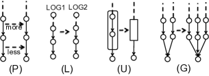
Figure 2: Dimensions of change for query revisions

(P) Parameters: The query parameters are modified to obtain slightly different results (Figure 2P). For example, the analyst may alter a selection predicate or a top-$k$ value to allow more or less data in the output.

(L) Logs: An analyst may make use of an additional data source in the query to obtain richer results (Figure 2L).

(U) UDFs: An analyst may add or replace a set of operations in the query with a specialized UDF.

(G) Sub-Goals: Typically, an analyst writes several sub-queries that each achieves a single goal and then joins these to obtain the final output (Figure 2G). A revision may add or remove a sub-goal.

These four dimensions {P,L,U,G} serve as our evolving query building blocks. For each query revision, the changes are expressed by one or more of these dimensions.

Table 1: Eight analyst marketing scenarios, along with the dimensions modified during each of the 4 evolutions

Analyst1 wants to identify a number of “wine lovers” to send them a coupon for a new wine being introduced in a local region. This evolution investigates ways of finding suitable users to whom sending a coupon would have the most impact.	$Q\rightarrow\{P,L,G\}\rightarrow\{P\}\rightarrow\{P,G\}$
Analyst 2 wants to find influential users who visit a lot of restaurants for inclusion in an advertisement campaign. The evolution of this scenario will focus on increasingly sophisticated ways of identifying users who are “foodies”.	$Q\rightarrow\{L,U,G\}\rightarrow\{P,G\}\rightarrow\{P,G\}$
Analyst3 wants to start a gift recommendation service where friends can send a gift certificate to a user $u_{1}$. We want to generate a few restaurant choices based on $u_{1}$’s preferences and his friend’s preferences. The evolution in this scenario will investigate how to generate a diverse set of recommendations that would cater to $u$ and his close set of friends.	$Q\rightarrow\{P,G\}\rightarrow\{P,L,G\}\rightarrow\{G\}$
Analyst4 wants to identify a good area to locate a sports bar. The area must have a lot of people who like sports and check-in to bars, but the area does not already have too many sports bars in relation to other areas. The evolution focuses on identifying a suitable area where there is high interest but a low density of sports bars.	$Q\rightarrow\{U,G\}\rightarrow\{L,U,G\}\rightarrow\{U,G\}$
Analyst5 wants to give restaurant owners a customer poaching tool. For each restaurant $r$, we identify customers who go to a “similar” restaurant in the area but do not visit $r$. The owner of $r$ may use this to target advertisements. The evolutionary nature focuses on determining “similar” restaurants and their users.	$Q\rightarrow\{L,G\}\rightarrow\{L,U\}\rightarrow\{P,G\}$
Analyst6 tries to find out if restaurants are losing loyal customers. He wants to identify those customers who used to visit more frequently but are now visiting other restaurants in the area so that he can send them a coupon to win them back. The evolutionary nature of this scenario will focus on how to identify prior active users.	$Q\rightarrow\{L,G\}\rightarrow\{P,G\}\rightarrow\{P,G\}$
Analyst7 wants to identify the direct competition for poorly-performing restaurants. He first tries to determine if there is a more successful restaurant of similar type in the same area. The evolutionary nature focuses on identifying good and bad restaurants in an area, as well as what customers like about the menu, food, service, etc. about the successful restaurants in the area.	$Q\rightarrow\{L,G\}\rightarrow\{G\}\rightarrow\{U,G\}$
Analyst8 wants to recommend a high-end hotel vacation in an area users will like based on their known preferences for restaurants, theaters, and luxury items. The evolutionary nature focuses on matching user’s preferences with the types of businesses in an area.	$Q\rightarrow\{L,G\}\rightarrow\{U,G\}\rightarrow\{P,L,U,G\}$

3.2 Queries

We give a high-level description of each query scenario in Table 1 left column, and the right column specifies the change from one version to the next in terms of our query building blocks. For instance, let $Q$ represent the analyst’s first version of the query. Then each subsequent version (i.e., 2,3,4) is represented by indicating the dimensions that were changed during each revision in the following way:

$$Q\rightarrow\{P,L,G\}\rightarrow\{P\}\rightarrow\{P,G\}$$ (1)

To illustrate this process, we start with Example 1 as the first version of Analyst 1’s query in Table 1. This version is indicated by $Q$ above. Analyst 1 first desires to find users who like wine, are affluent, and have many good friends.

Example 1

(a): EXTRACT user from Twitter log. Apply UDF-CLASSIFY-WINE-SCORE on each user tweet to obtain a wine-score. Groupby user, compute a wine-sentiment-score for each user.

(b): From Twitter log, apply UDAF-CLASSIFY-AFFLUENT on tweets to classify a user as affluent or not.

(c): From Twitter log, create social network between every user pair using tweet source and dest. GROUPBY user pair in social network, count tweets. Assign friendship-strength-score to each user pair.

JOIN (a),(b), and (c). Threshold based on wine-sentiment-score, friendship-strength-score.

Next the analyst wants to find more evidence that the user likes wine. She revises the query by changing {P,L,G}, adding two new data sources {$L$} (Foursquare and Landmarks), a new sub-goal {$G$} that computes a checkin-count for users who go to wine places, and decreases the threshold parameter {$P$} for wine-sentiment-score since she will have evidence a user likes wine from 2 data sources. Example 2 below describes version 2 of the query.

Example 2

(d): EXTRACT from Foursquare log. For each checkin, obtain the user and restaurant name. Using the Landmarks data, filter by checkin to places of type wine-bar. Groupby user, compute checkin-count.

(e): Decrease wine-sentiment-score threshold

JOIN (a),(b),(c) and (d). Threshold based on new wine-sentiment-score in (e), friendship-strength-score.

Query versions 3 and 4 are revised similarly but are omitted due to lack of space. A detailed description of all queries is provided in the extended version [14].

4 Running the Benchmark

We now present our benchmark methodology for query evolution, user evolution, and data evolution and we show an example of benchmark results. We consider the initial system state to be idle, with no previously loaded data or executed queries.

4.1 Benchmark methodology

Query evolution

This test will use all analysts 1–8 and all query versions from each analyst. (1) From initial system state, execute analyst 1 query versions 1 through 4 in succession, returning to initial system state before each version. (2) From initial system state, execute analyst 1 query versions 1 through 4 in succession, without returning to initial system state before each version. Compare metrics from (1) and (2), and repeat for each remaining analyst. This comparison highlights a system’s ability to process any repeating tasks from the same user.

User evolution

This test will use all analysts 1–8 but only version 1 of each analyst’s query. First, assume some order of analysts 1–8. (1) From initial system state, execute each analyst’s query in the chosen order, returning to initial system state before each query. (2) From initial system state, execute each analyst’s query in the chosen order, without returning to initial system state before each query. Compare metrics from (1) and (2). This comparison highlights a system’s ability to process similar tasks from different users.

Data evolution

This test will use a single data source, e.g., Twitter log, and the subset of data requested in the first step should be a number of columns equal to half of the total number of columns in the log schema. The columns should be randomly chosen each time. (1) From an initial system state, an analyst requests a subset of data from a new data source. (2) An analyst requests one additional attribute from the data source in (1), in each successive version of the query. (3) A new analyst requests a subset of data previously accessed by the analyst in (1). (4) Repeat (1), (2), (3) returning to the initial state after each query. Compare metrics from (1), (2), (3) with (4). This comparison highlights a system’s ability to access subsets of data from a new data source on demand.

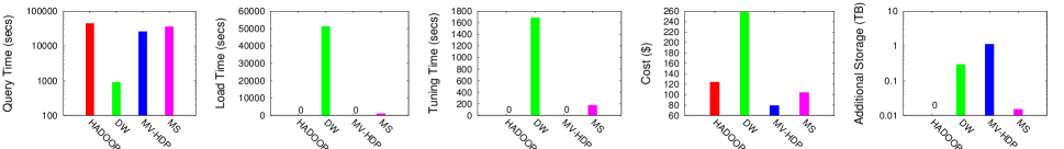
Figure 3: Figure shows a sample reporting of 4 data systems on a user evolution scenario

4.2 Example benchmark results

Next, we briefly show a sample reporting on the relative performance of four data systems using our workload and metrics for a user evolution scenario. The experimental setup consists of 9 nodes running a widely used commercial parallel data warehouse (DW) and 14 nodes running Hadoop. The ratio of Hadoop nodes to DW nodes is 1.5$\times$. The DW and Hadoop clusters are independent, and nodes are connected with 1 GbE. Each node has two 2.4 GHz xeon CPUs and a local 2 TB disk. In this test, our data includes a 1 TB Foursquare log, a 1 TB Twitter log and 12 GB Landmarks log. We use Hive [24] to execute our queries on the Hadoop system. Since all systems utilize the base data stored in Hadoop, we omit this from the storage metric.

Figure 3 reports the results for the user evolution scenario. HADOOP corresponds to a Hadoop-only execution of the query. DW executes the query on the DW but uses Hadoop as an ETL tool to extract the subset of data required by the query. MV-HDP corresponds to a system that we developed in [13] that rewrites Hadoop queries based on opportunistic materialistic views left behind from prior execution runs. MS is an implementation of a multi-store query optimizer (similar to [22]) that uses both Hadoop and a data warehouse together to execute each query. For MS, the load time refers only to the time to move and then load data on-the-fly from HADOOP to DW after partial execution in HADOOP.

It can be seen from the figure that reporting on the 5 metrics exposes their tradeoffs, which are not easily captured when reporting just on the query execution time. Since Hadoop performs ETL on the fly, query performance is quite poor compared to the DW. On the other hand, the superior performance of the DW is offset by the high cost of loading the data into the data warehouse. Both MV-HDP and MS show tradeoffs that reduce query response time. HADOOP and MV-HDP do not incur any tuning overhead whereas DW and MS require a tuning phase to provide good performance. We used Amazon EC2 and Redshift [1] pricing to approximate the dollar cost of the machines and storage (using cost for machines similar to those in our in-house clusters). The cost values show that HADOOP is far cheaper than DW while MS is cheaper than both, and MV-HDP has the lowest cost. Finally, it can be seen that MV-HDP incurs a significant storage overhead by retaining results as opportunistic views from all the prior executions runs. The tradeoff with storage size improves query response time compared to HADOOP.

5 Discussion

In the new analytical space, the key question is how to design systems to address emerging needs. The continued popularity of Hadoop and data warehouses notwithstanding, these are only suitable when the required use-case matches either of their starkly different characteristics. One focuses on being able to query the data right away, tolerating lesser performance. The other focuses on performance at the expense of significant delay in being able to query the data. These systems represent two ends of a spectrum, and the influx of so many new data processing systems shows that these two distinct choices are not meeting all current needs.

In this paper, our metrics highlight the tradeoffs among many design choices and the metrics can be used to guide system development. For example, we show 2 systems that remedy one dimension by shifting the tradeoff with another dimension. With MV-HDP we show that increased storage leads to better performance than Hadoop. With MS we show that one can remedy the loading time of a data warehouse to an extent by sacrificing some of DW performance. An interesting further research direction is to leverage the best properties of several systems to create hybrid systems.

6 Query Descriptions

In this section we describe each of the queries. These queries use three datasets: a Twitter data stream of user tweets, a Foursquare (4SQ) data stream of user checkins, and a Landmarks log of locations and their types. The identity of users is common across the Twitter and 4SQ logs, while identity of locations is common across the 4SQ and Landmarks logs. All logs are stored as json text.

We present 8 Analyst’s queries with 4 versions each. For each analyst, we state a high-level goal of what the analyst is trying to achieve, as well as 4 query versions toward the stated goal. Each query version modifies the previous version. For each query, we describe the task rather than provide an implementation in particular language since many are possible, e.g., SQL, HiveQL, Pig, Java, etc.

During a typical exploration, and analyst may spend a lot of time identifying the data distribution to get an understanding of where the density and sparsity lies. For this reason, the queries below have parameters indicated by an underline that an analyst would modify in order to obtain a representative answer set. Choosing an appropriate value or interpretation of the underlined parts of the queries is a necessary step an analyst performs. This may require a trial and error process resulting in additional versions of the queries. We leave these values unspecified as they are a function of the real-world datasets used.

Finally, it is important to note that the queries are not rigid interpretations of a goal, but rather one approach toward answering a question. For example, there may be several ways to interpret what it means to be “good” friends in a social network. Furthermore, even for a particular interpretation, there may be several ways to express it as a query. Hence, other variations of a query are possible.

User Defined Functions referenced by queries

The following queries reference multiple UDFs, for which we provide a brief description below. Text classifiers can be implemented using a bag-of-words method. For example, classes such as coffee-drinker may include the words (coffee, espresso, latte, french press) while wine-lover may include (cabernet, vineyard, merlot, chardonnay). By accepting a bag of words as an argument, these UDFs are easily reusable. However, this does not exclude other classification methods. UDAFs perform a groupby on a key and apply similar classification on the elements of a group.

1. UDF-CLASSIFY-WINE-SCORE: Input is text and output is wine-score indicating a strong presence of wine-terms.

2. UDF-CLASSIFY-FOOD-SCORE: Input is text and output is food-sentiment-score indicating a strong presence of food-terms.

3. UDF-GRID-CELL: Input is lat-lon coordinates and grid resolution, and output is a grid-cell number.

4. UDF-CLASSIFY-BEER-SCORE: Input is text and output is beer-score indicating a strong presence of beer-terms.

5. UDF-MENU-SIMILARITY: Input is two lists of menu items and output is a score indicating the similarity of the lists.

6. UDF-NLP-ENTITITY-SENTIMENT: Input is text and output is the entities extracted from the text with a sentiment-score for each entity.

7. UDF-CLASSIFY-LUXURY-SCORE: Input is text and output is a binary value indicating if the text concerns luxury items.

8. UDF-SENTIMENT: Input is text and output is a sentiment-score expressing positive or negative sentiment with the score indicating the strength of the sentiment.

9. UDAF-CLASSIFY-AFFLUENT: Input is all text from a given user and output is a binary value indicating if the user is affluent or not.

10. UDAF-CLASSIFY-SPORTS: Input is all text from a given user and output is a binary value indicating if the user is interested in sports or not.

6.1 Analyst 1

Analyst1 wants to identify a number of “wine lovers” to send them a coupon for a new wine being introduced in a local region. This evolution investigates ways of finding suitable users to whom sending a coupon would have the most impact.

6.1.1 Analyst 1, Version 1

• Analyst goal: Find users that like wine, have strong friendships, and are affluent.

• Query: From Twitter, apply UDF-CLASSIFY-WINE-SCORE on each user’s tweets and groupby user to produce wine-sentiment-score for each user. Threshold on wine-sentiment-score above $x_{1}$.

  From Twitter, compute all pairs $\langle u_{1},u_{2}\rangle$ of users that communicate with each other, assigning each pair a friendship-strength-score based on the number of times they communicate. Threshold on friendship-strength-score above $x_{2}$.

  From Twitter, apply UDAF-CLASSIFY-AFFLUENT on users and their tweets.

  Join results by user.

6.1.2 Analyst 1, Version 2

• Analyst goal: Next, consider users to be wine-lovers if they checkin to many wine places.

• Query: From previous version, reduce wine-sentiment-score threshold to $x_{2}^{\prime}$ since now there will be additional evidence a user likes wine.

  From 4SQ, identify places that users checkin. Join with places in Landmarks. Select users that checkin to places of type wine-bar. For each user, count the number of checkins. Threshold on checkin-count above $x_{3}$.

  Join these with users from previous version.

6.1.3 Analyst 1, Version 3

• Analyst goal: Now find users that are also in the San Francisco area as well as prolific on Twitter.

• Query: From previous version, select users local to San Francisco. Threshold on tweet-count above $x_{4}$. Adjust $x_{1}$, $x_{2}$, $x_{3}$ appropriately to produce “enough” answers.

6.1.4 Analyst 1, Version 4

• Analyst goal: Finally, require that a user’s friends must also visit wine-places.

• Query: For user pairs $\langle u_{1},u_{2}\rangle$, threshold on $u_{2}$ checkin-score above $x_{5}$. For each user $u_{1}$, count the number of friends with checkin-count above threshold. Retain $u_{1}$ if count above $x_{6}$. Join these with users from previous version.

6.2 Analyst 2

Analyst 2 wants to find influential users who visit a lot of restaurants for inclusion in an advertisement campaign. The evolution of this scenario will focus on increasingly sophisticated ways of identifying users who are “foodies”.

6.2.1 Analyst 2, Version 1

• Analyst goal: Find users who frequently visit restaurants.

• Query: From 4SQ, identify places that users checkin. Join with places in Landmark log. Select users that checkin to places of type restaurant. For each user, count the number of times they checkin to a place of type restaurant. Compute the normalized-count based on the maximum count across all users. Threshold on normalized-count above $x_{1}$.

6.2.2 Analyst 2, Version 2

• Analyst goal: Additionally, user also likes food if they talk positively about food.

• Query: From Twitter, apply UDF-CLASSIFY-FOOD-SCORE on each user’s tweets and groupby user to produce food-sentiment-score for each user. Threshold on food-sentiment-score above $x_{2}$.

  Join these users with users in previous version.

6.2.3 Analyst 2, Version 3

• Analyst goal: Further define that a user likes food if they dine at many different types of restaurants.

• Query: Revise previous version by counting the number of times a user has visited each distinct type of restaurant. Select users who have visited $x_{3}$ distinct restaurant types at least $x_{4}$ times.

6.2.4 Analyst 2, Version 4

• Analyst goal: Finally, require that these users do not frequently visit restaurants with low ratings.

• Query: From previous version, compute the percentage of each user’s checkins to restaurants with ratings less than $x_{5}$. Threshold on percent below $x_{6}$.

6.3 Analyst 3

Analyst3 wants to start a gift recommendation service where friends can send a gift certificate to a user $u$. We want to generate a few restaurant choices based on $u$’s preferences and $u$’s friend’s preferences. The evolution in this scenario will investigate how to generate a diverse set of recommendations that would cater to $u$, and $u$’s close set of friends.

6.3.1 Analyst 3, Version 1

• Analyst goal: For each user $u$, identify those restaurants that $u$’s good friends frequently visit.

• Query: From Twitter, compute all pairs $\langle u_{1},u_{2}\rangle$ of users that communicate with each other, assigning each pair a friendship-strength-score based on the number of times they communicate. Threshold on friendship-strength-score above $x_{1}$.

  From 4SQ, identify places that users checkin. Join with places in Landmarks. Select users that checkin to places of type restaurant.

  For each user $u_{1}$, find all the restaurants that her friends $u_{2}$ have visited. For each restaurant, count the number of checkins. Threshold on count above $x_{2}$.

6.3.2 Analyst 3, Version 2

• Analyst goal: Next, only consider users that have friends in the same area as well as other friends in common.

• Query: Revise the previous version by redefining what it means to be good friends. From Twitter, recompute all pairs $\langle u_{1},u_{2}\rangle$ of users that live in the same area, and have a friendship-strength-score above $x_{3}$. Additionally, a user pair $\langle u_{1},u_{2}\rangle$ are said to be good friends if they have more than $x_{4}$ friends in common.

6.3.3 Analyst 3, Version 3

• Analyst goal: Next, identify only those restaurants that are the same type as a user’s favorite restaurant.

• Query: From 4SQ, for each user $u_{1}$, find favorite restaurant type by counting the number of checkins to each restaurant, and select the restaurant with the max number of checkins as $u_{1}$’s favorite restaurant $r$.

  Join with Landmarks to obtain $r$’s type.

  From the previous version, select only those restaurants for $u_{1}$ that belong to the same type as $u_{1}$’s favorite type.

6.3.4 Analyst 3, Version 4

• Analyst goal: Finally, find additional restaurants that are similar to those visited by a user’s friends.

• Query: From 4SQ, for all restaurant pairs $\langle r_{1},r_{2}\rangle$, count the number of users that have visited both restaurants. Threshold on count above $x_{5}$. All remaining pairs $\langle r_{1},r_{2}\rangle$ are considered to be similar since they have many common customers. For each user $u_{1}$, suggest $r_{2}$ if $r_{1}$ is a restaurant frequently visited by $u_{1}$’s friends.

6.4 Analyst 4

Analyst4 wants to identify a good area to locate a sports bar. The area must have a lot of people who like sports and check-in to bars, but the area does not already have too many sports bars in relation to other areas. The evolution focuses on identifying a suitable area where there is high interest but a low density of sports bars.

6.4.1 Analyst 4, Version 1

• Analyst goal: Find users who like beer and where they live.

• Query: From 4SQ, identify users and their location that frequently mention the word “beer” in their text. For each user, count the occurrences of the word. Threshold on count above $x_{1}$.

6.4.2 Analyst 4, Version 2

• Analyst goal: Next, find areas where there are many beer lovers.

• Query: From the previous version, use UDF-GRID-CELL to map user locations to a grid cell. Count number of users in each grid cell. Threshold on count above $x_{2}$.

6.4.3 Analyst 4, Version 3

• Analyst goal: Next, find areas with many users that like beer and sports but do not have many sports bars.

• Query: From Twitter, apply UDAF-CLASSIFY-SPORTS on users and their tweets. Then apply a UDF-CLASSIFY-BEER-SCORE to better identify users that like beer, and produce a beer-score for each user. Join sports and beer users. Threshold on beer-score above $x_{3}$. Next, apply UDF-GRID-CELL to map user locations to a grid cell. Count number of users in each grid cell. Threshold on count above $x_{4}$.

  From Landmarks, obtain restaurant name, type and location. Select places that are type equal to sports bar. Next, apply UDF-GRID-CELL to map place locations to a grid cell. Count number of restaurants in each grid cell. Threshold on count below $x_{5}$.

  Join grid cells from user locations and sports bar locations.

6.4.4 Analyst 4, Version 4

• Analyst goal: Finally, find area with high user interest but few popular sports bars relative to the number of users.

• Query: From 4SQ, identify places that users checkin.

  Join with places in Landmarks. Select places that are type equal to sports bar. For each place, count the number of checkins. Threshold on count above $x_{6}$.

  Next, apply UDF-GRID-CELL to map place locations to a grid cell. Count the number of places per grid cell.

  Join this with the grid cells from previous version. Threshold on ratio of user to sports bars count above $x_{7}$.

6.5 Analyst 5

Analyst5 wants to give restaurant owners a customer poaching tool. For each restaurant $r$, we identify customers who go to a “similar” restaurant in the area but do not visit $r$. The owner of $r$ may use this to target advertisements. The evolutionary nature focuses on determining “similar” restaurants and their users.

6.5.1 Analyst 5, Version 1

• Analyst goal: Find similar restaurants based the overlap of users that checkin to each place.

• Query: From 4SQ, for all restaurant pairs $\langle r_{1},r_{2}\rangle$, count the number of users that have visited both restaurants. Threshold on count above $x_{1}$.

6.5.2 Analyst 5, Version 2

• Analyst goal: Next, find restaurants that are similar as indicated by a user or the user’s friends frequently visiting the same places.

• Query: From Twitter, compute all pairs $\langle u_{1},u_{2}\rangle$ of users that communicate with each other, assigning each pair a friendship-strength-score based on the number of times they communicate. Threshold on friendship-strength-score above $x_{2}$.

  From 4SQ, for all restaurant pairs $\langle r_{1},r_{2}\rangle$, count the number of users that have visited both restaurants, as well as the number of times a user $u_{1}$ has visited $r_{1}$ and one of their friends $u_{2}$ has visited $r_{2}$. Threshold on count above $x_{3}$.

6.5.3 Analyst 5, Version 3

• Analyst goal: Next, find restaurant pairs that are also similar based on the similarity of their menus.

• Query: From Landmarks, create restaurant pairs $\langle r_{1}^{\prime},r_{2}^{\prime}\rangle$ that have the same zip code and type. For each pair, apply UDF-MENU-SIMILARITY to obtain menu-similarity-score. Threshold on menu-similarity-score above $x_{4}$.

  Join pairs $\langle r_{1}^{\prime},r_{2}^{\prime}\rangle$ with pairs $\langle r_{1},r_{2}\rangle$ from the previous version.

6.5.4 Analyst 5, Version 4

• Analyst goal: Finally, find users that visit one restaurant but not a similar restaurant.

• Query: From 4SQ, for each restaurant $r$, identify the users that have visited $r$ and the count of times they have visited. For each restaurant pair $\langle r_{1},r_{2}\rangle$ from the previous version, select users $u$ that have visited $r_{1}$ more than $x_{5}$ times and visited $r_{2}$ less than $x_{6}$ times.

6.6 Analyst 6

Analyst6 tries to find out if restaurants are losing loyal customers. He wants to identify those customers who used to visit more frequently but are now visiting other restaurants in the area so that he can send them a coupon to win them back. The evolutionary nature of this scenario will focus on how to identify prior active users.

6.6.1 Analyst 6, Version 1

• Analyst goal: For each restaurant, identify other restaurants with the same zip code and type that are less popular.

• Query: From Landmarks, create restaurant pairs $\langle r_{1},r_{2}\rangle$ that have the same zip code and type, and $r_{2}$ has a much lower checkin count than $r_{1}$.

6.6.2 Analyst 6, Version 2

• Analyst goal: Now, identify restaurants that have lately become less popular.

• Query: From 4SQ, identify places that users checkin.

  Join with places in Landmarks that have type restaurant. For each restaurant, compute the average number of checkins per month in the last $x_{1}$ months and the number of checkins in the last 1 month.

  Threshold on the ratio of recent checkins to historical average checkins below $x_{2}$.

6.6.3 Analyst 6, Version 3

• Analyst goal: Next, find users that stopped visiting those restaurants.

• Query: For restaurant $r$ identified as becoming less popular in the previous version, and a user $u$ that visited $r$, compute the average number of checkins per month by user $u$ in the last $x_{3}$ months and the number of checkins by user $u$ in the last 1 month. Compute the ratio of recent checkins to historical average checkins

  Threshold on ratio below $x_{4}$.

6.6.4 Analyst 6, Version 4

• Analyst goal: Finally, find users that no longer frequent a particular restaurant but still visit other restaurants in the same area.

• Query: From 4SQ, for each user $u$, count the number of checkins by zip code. Threshold on count above $x_{5}$.

  For each less popular restaurant $r$ identified in previous version, retain $u$ only if $u$ still frequently visits restaurants in the same zip code as $r$.

6.7 Analyst 7

Analyst7 wants to identify the direct competition for poorly-performing restaurants. He first tries to determine if there is a more successful restaurant of similar type in the same area. The evolutionary nature focuses on identifying good and bad restaurants in an area, as well as what customers like about the menu, food, service, etc. about the successful restaurants in the area.

6.7.1 Analyst 7, Version 1

• Analyst goal: For each zip code, identify good and bad restaurants.

• Query: From Landmarks, identify places that are restaurants, and apply UDF-SENTIMENT on the restaurant comments to obtain a sentiment-score. For each zip code, retain restaurants with sentiment-score above $x_{1}$ or below $x_{2}$ as good and bad restaurants.

6.7.2 Analyst 7, Version 2

• Analyst goal: Next, refine the discrimination of restaurants as good and bad based on their popularity.

• Query: From 4SQ, obtain the checkin count for every restaurant.

  Threshold on count above $x_{3}$. Join with the good restaurants from the previous version.

  Threshold on count below $x_{4}$. Join with the bad restaurants from the previous version.

6.7.3 Analyst 7, Version 3

• Analyst goal: Further discriminate restaurants as good and bad based repeat checkins.

• Query: From 4SQ, obtain the checkin count for every restaurant. For each restaurant, count the number of users that checkedin only once, and the number of users that checkedin more than $x_{5}$ times. Compute the ratio of single checkins to multiple checkins.

  Threshold on ratio below $x_{6}$. Join with the good restaurants from the previous version.

  Threshold on ratio above $x_{7}$. Join with the bad restaurants from the previous version.

6.7.4 Analyst 7, Version 4

• Analyst goal: Next, for each restaurant, find the most frequent entities with positive and negative comments.

• Query: From 4SQ, apply UDF-NLP-ENTITITY-SENTIMENT per user checkin. For each restaurant and each entity, aggregate the sentiment-score. Threshold on sentiment-score above $x_{5}$.

  Join with good and bad restaurants from previous version.

6.8 Analyst 8

Analyst8 wants to recommend a high-end hotel vacation in an area users will like based on their known preferences for restaurants, theaters, and luxury items. The evolutionary nature focuses on matching user’s preferences with the types of businesses in an area.

6.8.1 Analyst 8, Version 1

• Analyst goal: Find users who talk about ‘luxury items’.

• Query: From Twitter, apply UDF-CLASSIFY-LUXURY-SCORE on user tweets. For each user, count the number of tweets about luxury-items. Threshold on count above $x_{1}$.

6.8.2 Analyst 8, Version 2

• Analyst goal: Next, identify restaurants those users frequently visit.

• Query: From 4SQ, for each user, count the number of checkins per restaurant. Threshold on count above $x_{2}$.

  Join with users from previous version.

  For each restaurant, count the total number of checkins by all these users. Threshold on count above $x_{3}$.

6.8.3 Analyst 8, Version 3

• Analyst goal: Next, find areas that have a high density of these restaurants and identify the distribution of restaurant types in the area.

• Query: For the restaurants from the previous version, apply UDF-GRID-CELL. Count the number of restaurants per grid cell. Threshold on count above $x_{4}$.

  For each grid cell, compute a histogram on the restaurant type and count.

6.8.4 Analyst 8, Version 4

• Analyst goal: Finally, match users to grid cells and find luxury hotels in their matching grid cell.

• Query: For each user $u$ from previous version, identify location, and compute a histogram on the restaurant type and $u$’s checkin count.

  Match $u$ to a grid cell such that the grid cell is sufficiently far away from $u$’s location, and there is a significant overlap between $u$’s histogram and grid-cell $g$ histogram from previous version.

  From Landmarks, find hotels with rating greater than $x_{5}$ stars, and apply UDF-GRID-CELL to convert hotel location to grid cell $g^{\prime}$.

  For each user $u$, join grid cell $g$ with $g^{\prime}$ to identify hotels in an area matching $u$’s restaurant preferences.

References

- [1] Amazon Web Services (EC2, RDS, Redshift). http://aws.amazon.com/.
- [2] Apache Mahout. http://mahout.apache.org/, 2010.
- [3] D. Bowie. Do you need a data scientist? CIO, Sept. 2012.
- [4] G. Chatzopoulou, M. Eirinaki, and N. Polyzotis. Query recommendations for interactive database exploration. In SSDBM, 2009.
- [5] J. Cohen, B. Dolan, M. Dunlap, J. M. Hellerstein, and C. Welton. MAD Skills: new analysis practices for big data. VLDB, 2(2):1481–1492, 2009.
- [6] M. Franklin, A. Halevy, and D. Maier. From databases to dataspaces: a new abstraction for information management. ACM Sigmod Record, 34(4):27–33, 2005.
- [7] Google Compute Engine. https://cloud.google.com/products/compute-engine.
- [8] T. Groenfeldt. Big data knows you, even if you don’t know big data. Forbes, Nov. 2011.
- [9] J. M. Hellerstein, C. Ré, F. Schoppmann, D. Z. Wang, E. Fratkin, A. Gorajek, K. S. Ng, C. Welton, X. Feng, K. Li, et al. The MADlib analytics library: or MAD skills, the SQL. VLDB, 5(12):1700–1711, 2012.
- [10] D. Henschen. IBM beats Oracle, Microsoft with big data leap. InformationWeek, Oct. 2011.
- [11] N. Khoussainova, M. Balazinska, W. Gatterbauer, Y. Kwon, and D. Suciu. A case for a collaborative query management system. In CIDR, 2009.
- [12] S. LaValle, E. Lesser, R. Shockley, M. Hopkins, and N. Kruschwitz. Big data, analytics and the path from insights to value. MIT Sloan Management Review, 52(2):21–32, 2011.
- [13] J. LeFevre, J. Sankaranarayanan, H. Hacıgümüş, J. Tatemura, and N. Polyzotis. Exploiting opportunistic physical design in large-scale data analytics. CoRR, 2013.
- [14] J. LeFevre, J. Sankaranarayanan, H. Hacıgümüş, J. Tatemura, and N. Polyzotis. Towards a workload for evolutionary analytics. CoRR, 2013.
- [15] LinkedIn. http://data.linkedin.com/opensource/datafu, 2011.
- [16] Microsoft Windows Azure. http://www.windowsazure.com/.
- [17] MyExperiment. http://myexperiment.org/workflows.
- [18] H. Park, R. Ikeda, and J. Widom. RAMP: A system for capturing and tracing provenance in MapReduce workflows. VLDB, 4(12), 2011.
- [19] D. Patil. Building Data Science Teams. O’Reilly, 2011.
- [20] A. Pavlo, E. Paulson, A. Rasin, D. J. Abadi, D. J. DeWitt, S. Madden, and M. Stonebraker. A comparison of approaches to large-scale data analysis. In SIGMOD, 2009.
- [21] T. Sellam and M. Kersten. Meet Charles, big data query advisor. In CIDR, 2013.
- [22] A. Simitsis, K. Wilkinson, M. Castellanos, and U. Dayal. Optimizing analytic data flows for multiple execution engines. In ICDE, pages 829–840, 2012.
- [23] Taverna Workflow Management System. http://www.taverna.org.uk.
- [24] A. Thusoo, Z. Shao, S. Anthony, D. Borthakur, N. Jain, J. Sen Sarma, R. Murthy, and H. Liu. Data warehousing and analytics infrastructure at facebook. In SIGMOD, 2010.
- [25] Transaction Processing Peformance Council. www.tpc.org.
- [26] Yahoo! Pipes. http://pipes.yahoo.com.