Stochastic Analysis on RAID Reliability for Solid-State Drives

Abstract

Solid-state drives (SSDs) have been widely deployed in desktops and data centers. However, SSDs suffer from bit errors, and the bit error rate is time dependent since it increases as an SSD wears down. Traditional storage systems mainly use parity-based RAID to provide reliability guarantees by striping redundancy across multiple devices, but the effectiveness of RAID in SSDs remains debatable as parity updates aggravate the wearing and bit error rates of SSDs. In particular, an open problem is that how different parity distributions over multiple devices, such as the even distribution suggested by conventional wisdom, or uneven distributions proposed in recent RAID schemes for SSDs, may influence the reliability of an SSD RAID array. To address this fundamental problem, we propose the first analytical model to quantify the reliability dynamics of an SSD RAID array. Specifically, we develop a “non-homogeneous” continuous time Markov chain model, and derive the transient reliability solution. We validate our model via trace-driven simulations and conduct numerical analysis to provide insights into the reliability dynamics of SSD RAID arrays under different parity distributions and subject to different bit error rates and array configurations. Designers can use our model to decide the appropriate parity distribution based on their reliability requirements.

I Introduction

Solid-state drives (SSDs) emerge to be the next-generation storage medium. Today’s SSDs mostly build on NAND flash memories, and provide several design enhancements over hard disks including higher I/O performance, lower energy consumption, and higher shock resistance. As SSDs continue to see price drops nowadays, they have been widely deployed in desktops and large-scale data centers [10, 14].

However, even though enterprise SSDs generally provide high reliability guarantees (e.g., with mean-time-between-failures of 2 million hours [17]), they are susceptible to wear-outs and bit errors. First, SSDs regularly perform erase operations between writes, yet they can only tolerate a limited number of erase cycles before wearing out. For example, the erasure limit is only 10K for multi-level cell (MLC) SSDs [5], and even drops to several hundred for the latest triple-level cell (TLC) SSDs [13]. Also, bit errors are common in SSDs due to read disturbs, program disturbs, and retention errors [27, 12, 13]. Although in practice SSDs use error correction codes (ECCs) to protect data [8, 26], the protection is limited since the bit error rate increases as SSDs issue more erase operations [27, 12]. We call a post-ECC bit error an uncorrectable bit error. Furthermore, bit errors become more severe when the density of flash cells increases and the feature size decreases [13]. Thus, SSD reliability remains a legitimate concern, especially when an SSD issues frequent erase operations due to heavy writes.

RAID (redundant array of independent disks) [31] provides an option to improve reliability of SSDs. Using parity-based RAID (e.g., RAID-4, RAID-5), the original data is encoded into parities, and the data and parities are striped across multiple SSDs to provide storage redundancy against failures. RAID has been widely used in tolerating hard disk failures, and conventional wisdom suggests that parities should be evenly distributed across multiple drives so as to achieve better load balancing, e.g., RAID-5. However, traditional RAID introduces a different reliability problem to SSDs since parities are updated for every data write and this aggravates the erase cycles. To address this problem, authors in [2] propose a RAID scheme called Diff-RAID which aims to enhance the SSD RAID reliability by keeping uneven parity distributions. Other studies (e.g., [16, 20, 21, 22, 30, 25]) also explore the use of RAID in SSDs.

However, there remain open issues on the proper architecture designs of highly reliable SSD RAID [19]. One specific open problem is how different parity distributions generally influence the reliability of an SSD RAID array subject to different error rates and array configurations. In other words, should we distribute parities evenly or unevenly across multiple SSDs with respect to the SSD RAID reliability? This motivates us to characterize the SSD RAID reliability using analytical modeling, which enables us to readily tune different input parameters and determine their impacts on reliability. However, analyzing the SSD RAID reliability is challenging, as the error rates of SSDs are time-varying. Specifically, unlike hard disk drives in which error arrivals are commonly modeled as a constant-rate Poisson process (e.g., see [33, 28]), SSDs have an increasing error arrival rate as they wear down with more erase operations.

In this paper, we formulate a continuous time Markov chain (CTMC) model to analyze the effects of different parity placement strategies, such as traditional RAID-5 and Diff-RAID [2], on the reliability dynamics of an SSD RAID array. To capture the time-varying bit error rates in SSDs, we formulate a non-homogeneous CTMC model, and conduct transient analysis to derive the system reliability at any specific time instant. To our knowledge, this is the first analytical study on the reliability of an SSD RAID array.

In summary, this paper makes two key contributions:

• We formulate a non-homogeneous CTMC model to characterize the reliability dynamics of an SSD RAID array. We use the uniformization technique [7, 18, 32] to derive the transient reliability of the array. Since the state space of our model increases with the SSD size, we develop optimization techniques to reduce the computational cost of transient analysis. We also quantify the corresponding error bounds of the uniformization and optimization techniques. Using the SSD simulator [1], we validate our model via trace-driven simulations.

• We conduct extensive numerical analysis to compare the reliability of an SSD RAID array under RAID-5 and Diff-RAID [2]. We observe that Diff-RAID, which places parities unevenly across SSDs, only improves the reliability over RAID-5 when the error rate is not too large, while RAID-5 is reliable enough if the error rate is sufficiently small. On the other hand, when the error rate is very large, neither RAID-5 nor Diff-RAID can provide high reliability, so increasing fault tolerance (e.g., RAID-6 or a stronger ECC) becomes necessary.

The rest of this paper proceeds as follows. In Section II, we formulate our model that characterizes the reliability dynamics of an SSD RAID array, and formally define the reliability metric. In Section III, we derive the transient system state using uniformization and some optimization techiniques. In Section IV, we validate our model via trace-driven simulations. In Section V, we present numerical analysis results on how different parity placement strategies influence the RAID reliability. Section VI reviews related work, and finally Section VII concludes.

II System Model

It is well known that RAID-5 is effective in providing single-fault tolerance for traditional hard disk storage. It distributes parities evenly across all drives and achieves load balancing. Recently, Balakrishnan et al. [2] report that RAID-5 may result in correlated failures, and hence poor reliability, for SSD RAID arrays if SSDs are worn out at the same time. Thus, they propose a modified RAID scheme called Diff-RAID for SSDs. Diff-RAID improves RAID-5 through (i) distributing parties unevenly and (ii) redistributing parities each time when a worn-out SSD is replaced so that the oldest SSD always has the most parities and wears out first. However, it remains unclear whether Diff-RAID (or placing parities unevenly across drives) really improves the reliability of SSD RAID over RAID-5 in all error patterns, as there is a lack of comprehensive studies on the reliability dynamics of SSD RAID arrays under different parity distributions.

In this section, we first formulate an SSD RAID array, then characterize the age of each SSD based on the age of the array (we will formally define the concept of age in later part of this section). Lastly, we model the error rate based on the age of each SSD, and formulate a non-homogeneous CTMC to characterize the reliability dynamics of an SSD RAID array under various parity distributions, including different parity placement distributions like RAID-5 or Diff-RAID. Table I lists the major notations used in this paper.

Specific Notations of SSD
$M$	:	Erasure limit of each block (e.g., 10K)
$B$	:	Total number of blocks in each SSD
$\lambda_{i}(t)$	:	Error rate of a chunk in SSD $i$ at time $t$
Specific Notations of RAID Array
$N$	:	Number of data drives (i.e., an array has $N+1$ SSDs)
$S$	:	Total number of stripes in an SSD RAID array
$p_{i}$	:	Fraction of parity chunks in SSD $i$, and $\sum_{i=0}^{N}p_{i}=1$
$k$	:	Total number of erasures performed on SSD RAID array (i.e., system age of the array)
$k_{i}$	:	Number of erasures performed on each block of SSD $i$ (i.e., age of SSD $i$)
$T$	:	Average inter-arrival time of two consecutive erasure operations on SSD RAID array
$\pi_{j}\!(t)$	:	Probability that the array has $j$ stripes that contain exactly one erroneous chunk each, ($0\leq j\leq S$)
$\!\!\pi\!_{S\!+\!1}\!(t)$	:	Probability that at least one stripe of the array contains more than one erroneous chunk, so $\sum_{j=0}^{S+1}\pi_{j}(t)=1$
$R(t)$	:	Reliability at time $t$, i.e., probability that no data loss happens until time $t$, $R(t)=\sum_{j=0}^{S}\pi_{j}(t)$

TABLE I: Notations.

II-A SSD RAID Formulations

An SSD is usually organized in blocks, each of which typically contains 64 or 128 pages. Both read and program (write) operations are performed in unit of pages, and each page is of size 4KB. Data can only be programmed to clean pages. SSDs use an erase operation, which is performed in unit of blocks, to reset all pages in a block into clean pages. To improve write performance, SSDs use out-of-place writes, i.e., to update a page, the new data is programmed to a clean page while the original page is marked as invalid. An SSD is usually composed of multiple chips (or packages), each containing thousands of blocks. Chips are independent of each other and can operate in parallel. We refer readers to [1] for a detailed description about the SSD organization.

We now describe the organization of an SSD RAID array that we consider, as shown in Figure 1. We consider the device-level RAID organization where the array is composed of $N\!+\!1$ SSDs numbered from 0 to $N$. In this paper, we address the case where the array is tolerable against a single SSD failure, as assumed in traditional RAID-4, RAID-5 schemes and the modified RAID schemes for SSDs [2, 16, 21, 22, 30, 20, 25]. Each SSD is divided into multiple non-overlapping chunks, each of which can be mapped to one or multiple physical pages. The array is further divided into stripes, each of which is a collection of $N+1$ chunks from the $N+1$ SSDs. Within a stripe, there are $N$ data chunks, and one parity chunk encoded from the $N$ data chunks. We call a chunk an erroneous chunk when uncorrectable bit errors appear in that chunk; or a correct chunk otherwise. Since we focus on single-fault tolerance, we require that each stripe contains at most one erroneous chunk without data loss so that it can be recovered from other surviving chunks in the same stripe.

Suppose that each SSD contains $B$ blocks, and the array contains $S$ stripes (i.e., $S$ chunks per SSD). For simplicity, we assume that all $S$ stripes are used for data storage. To generalize our analysis, we organize parity chunks in the array according to some probability distribution. We let SSD $i$ contain a fraction $p_{i}$ of parity chunks. In the special case of RAID-5, parity chunks are evenly placed across all devices, so $p_{i}=\frac{1}{N+1}$ for all $i$ if the array consists of $N+1$ drives. For Diff-RAID, $p_{i}$’s do not need to be equal to $\frac{1}{N+1}$, but only need to satisfy the condition of $\sum_{i=0}^{N}p_{i}=1$.

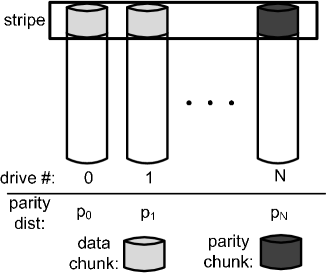
Figure 1: Organization of an SSD RAID array.

Each block in an SSD can only sustain a limited number of erase cycles, and is supposed to be worn out after the limit. We denote the erasure limit by $M$, which corresponds to the lifetime of a block. To enhance the durability of SSDs, efficient wear-leveling techniques are often used to balance the number of erasures across all blocks. In this paper, we assume that each SSD achieves perfect wear-leveling such that every block has exactly the same number of erasures. Let $k_{i}$ ($\leq M$) be the number of erasures that have been performed on each block in SSD $i$, where $0\leq i\leq N$. We denote $k_{i}$ as the age of each block in SSD $i$, or equivalently, the age of SSD $i$ when perfect wear-leveling is assumed. When an SSD reaches its erasure limit, we assume that it is replaced by a new SSD. For simplicity, we treat $k_{i}$ as a continuous value in $[0,M]$. Let $k$ be the total number of erase operations that the whole array has processed, and we call $k$ the system age of the array.

II-B SSD Age Characterization

In this subsection, we proceed to characterize the age of each SSD for a given RAID scheme. In particular, we derive $k_{i}$, denoting the age of SSD $i$, when the whole array has already performed a total of $k$ erase operations. This characterization enables us to model the error rate in each SSD accurately (see Section II-C). We focus on two RAID schemes: traditional RAID and Diff-RAID [2].

We first quantify the aging rate of each SSD in an array. Let $r_{i}$ be the aging rate of SSD $i$. Note that for each stripe, updating a data chunk also has the parity chunk updated. Suppose that each data chunk has the same probability of being accessed. On average, the ratio of the aging rate of SSD $i$ to that of SSD $j$ can be expressed as [2]:

$$\frac{r_{i}}{r_{j}}=\frac{p_{i}N+(1-p_{i})}{p_{j}N+(1-p_{j})}.$$ (1)

Equation (1) states that the parity chunk ages $N$ times faster than each data chunk. Given the aging rates $r_{i}$’s, we can quantify the probability of SSD $i$ being the target drive for each erase operation, which we denote by $q_{i}$. We model $q_{i}$ by making it proportional to the aging rate of SSD $i$, i.e.,

$$q_{i}=\frac{r_{i}}{\sum_{i=0}^{N}r_{i}}=\frac{p_{i}N+(1-p_{i})}{\sum_{i=0}^{N}(p_{i}N+(1-p_{i}))}.$$ (2)

We now characterize the age of Diff-RAID which places parities unevenly and redistributes parity chunks after the worn-out SSD is replaced so as to maintain the age ratios and always wear out the oldest SSD first. To mathematically characterize the system age of Diff-RAID, define $A_{i}$ as the remaining fraction of erasures that SSD $i$ can sustain right after an SSD replacement. Clearly, $A_{i}=1$ for a brand-new drive and $A_{i}=0$ for a worn-out drive. Without loss of generality, we assume that the drives are sorted by $A_{i}$ in descending order, i.e., $A_{0}\geq A_{1}\geq\cdots\geq A_{N}$, and we have $A_{0}=1$ as it is the newly replaced drive. Diff-RAID performs parity redistribution to guarantee that the aging ratio in Equation (1) remains unchanged. Therefore, the remaining fraction of erasures for each drive will converge, and the values of $A_{i}$’s in the steady state are given by [2]:

$$A_{i}\!=\!\frac{\sum_{j=i}^{N}r_{j}}{\sum_{j=0}^{N}r_{j}}\!=\!\frac{\sum_{j=i}^{N}(p_{j}N\!+\!(1\!-\!p_{j}))}{\sum_{j=0}^{N}(p_{j}N\!+\!(1\!-\!p_{j}))},\quad 0\!\leq\!i\!\leq\!N.$$ (3)

In this paper, we study Diff-RAID after the age distribution of SSDs right after each drive replacement converges, i.e., the initial remaining fractions of erasures of SSDs in Diff-RAID follow the distribution of $A_{i}$’s in Equation (3).

We now characterize $k_{i}$ for Diff-RAID. Recall that each SSD has $B$ blocks. Due to perfect wear-leveling, every block of SSD $i$ has the same probability $q_{i}/B$ of being the target block for an erase operation. Thus, if the array has processed $k$ erase operations, the age of SSD $i$ is:

$$\mbox{{\bf Diff-RAID:}}\quad k_{i}=\Big{(}\frac{kq_{i}}{B}\ \mbox{\sf mod}\ \frac{q_{i}}{q_{N}}(M\!-\!k_{N0})\Big{)}\!+\!k_{i0},$$ (4)

where $k_{i0}=M(1\!-\!A_{i})$ is the initial number of times that each block of SSD $i$ has been erased right after a drive replacement, and the notation mod denotes the modulo operation. The rationale of Equation (4) is as follows. Since we sort the SSDs by $A_{i}$ in descending order, SSD $N$ always has the highest aging rate and will be replaced first. Thus, after each block of SSD $N$ has performed $(M\!-\!k_{N0})$ erasures, SSD $N$ will be replaced, and each block of SSD $i$ has just been erased $\frac{q_{i}}{q_{N}}(M\!-\!k_{N0})$ times. Therefore, for SSD $i$, a drive replacement happens when each block has been erased every $\frac{q_{i}}{q_{N}}(M-k_{N0})$ times. Moreover, the initial number of erasures on each block of SSD $i$ right after a drive replacement is $k_{i0}$. Thus, the age of SSD $i$ is derived as in Equation (4). Since $k_{i0}=M(1-A_{i})$ and $A_{N}=q_{N}$, Equation (4) can be rewritten as:

$$\mbox{{\bf Diff-RAID:}}\quad k_{i}=\left((kq_{i}/B)\ \mbox{\sf mod}\ Mq_{i}\right)+M(1-A_{i}).$$ (5)

For traditional RAID (e.g., RAID-4 or RAID-5), parity chunks are kept intact, and will not be redistributed after a drive replacement. So after the array has performed $k$ erase operations, each block of SSD $i$ has just performed $kq_{i}/B$ erasures, and an SSD will be replaced every time when each block performed $M$ erasures. Thus, the age of SSD $i$ is:

$$\mbox{{\bf Traditional RAID:}}\quad k_{i}=(kq_{i}/B)\ \mbox{\sf mod}\ M.$$ (6)

II-C Continuous Time Markov Chain (CTMC)

We first model the error rate of an SSD. We assume that the error arrival processes of different chunks in an SSD are independent. Since different chunks in an SSD have the same age, they must have the same error rate. We let $\lambda_{i}(t)$ represent the error rate of each chunk in SSD $i$ at time $t$, and model it as a function of the number of erasures on SSD $i$ at time $t$, which is denoted by $k_{i}(t)$ (the notation $t$ may be dropped if the context is clear). Furthermore, to reflect that bit errors increase with the number of erasures, we model the error rate based on a Weibull distribution [34], which has been widely used in reliability engineering. Formally,

$$\lambda_{i}(t)=c\alpha(k_{i}(t))^{\alpha-1},\quad\alpha\!>\!1,$$ (7)

where $\alpha$ is called the shape parameter and $c$ is a constant.

Note that even if the error rates of SSDs are time-varying, they only vary with the number of erasures on the SSDs. If we let $t_{k}$ be the time point of the $k^{th}$ erasure on the array, then during the period $(t_{k},t_{k+1})$ (i.e., between the $k^{th}$ and $(k+1)^{th}$ erasures), the number of erasures on each SSD is fixed, hence the error rates during this period should be constant, and the error arrivals can be modeled as a Poisson process. In particular, $k_{i}(t)=k_{i}(k)$ if $t\in(t_{k},t_{k+1})$, and the function $k_{i}(k)$ is expressed by Equation (5) and (6).

We now formulate a CTMC model to characterize the reliability dynamics of an SSD RAID array. Recall that the array provides single-fault tolerance for each stripe. We say that the CTMC is at state $i$ if and only if the array has $i$ stripes that contain exactly one erroneous chunk each, where $0\!\leq\!i\!\leq\!S$. Data loss happens if any one stripe contains more than one erroneous chunk, and we denote this state by $S\!+\!1$. Let $X(t)$ be the system state at time $t$. Formally, we have $X(t)\in\{0,1,...,S+1\},\forall t\geq 0.$ To derive the system state, we let $\pi_{j}(t)$ be the probability that the CTMC is at state $j$ at time $t$ ($0\!\leq\!j\!\leq\!S\!+\!1$), so the system state can be characterized by the vector $\boldsymbol{\pi}(t)=(\pi_{0}(t),\pi_{1}(t),...,\pi_{S+1}(t))$.

Let us consider the transition of the CTMC. For each stripe, if it contains one erroneous chunk, then the erroneous chunk can be reconstructed from the other surviving chunks in the same stripe. Assume that only one stripe can be reconstructed at a time, and that the reconstruction time follows an exponential distribution with rate $\mu$. The state transition diagram of the CTMC is depicted in Figure 2. To elaborate, suppose that the RAID array is currently at state $j$, if an erroneous chunk appears in one of the $(S\!-\!j)$ stripes that originally have no erroneous chunk, then it will move to state $j\!+\!1$ with rate $(S\!-\!j)\sum_{i=0}^{N}\lambda_{i}(t)$; if an erroneous chunk appears in one of the $j$ stripes that already have another erroneous chunk, then the system will move to state $S\!+\!1$ (in which data loss occurs) with rate $j\sum_{i=0}^{N}\lambda_{i}(t)$.

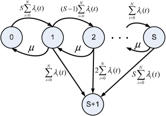
Figure 2: State transition of the non-homogeneous CTMC.

We now define the reliability of an SSD RAID array at time $t$, and denote it by $R(t)$. Formally, it is the probability that no stripe has encountered data loss until time $t$.

$$R(t)=\sum\nolimits_{j=0}^{S}\pi_{j}(t).$$ (8)

Note that our model captures the time-varying nature of reliability over the lifespan of the SSD RAID array. Next, we show how to analyze this non-homogeneous CTMC.

III Transient Analysis of CTMC

In this section, we derive $\boldsymbol{\pi}(t)$, the system state of an SSD RAID array at any time $t$. Once we have $\boldsymbol{\pi}(t)$, we can then compute the instantaneous reliability $R(t)$ according to Equation (8). There are two major challenges in deriving $\boldsymbol{\pi}(t)$. First, it involves transient analysis, which is different from the conventional steady state Markov chain analysis. Second, the underlying CTMC $\{X(t),t\geq 0\}$ is non-homogeneous, as the error arrival rate $\lambda_{i}(t)$ is time varying, and it also has a very large state space.

In the following, we first present the mathematical foundation on analyzing the non-homogeneous CTMC so as to compute the transient system state, then formalize an algorithm based on the mathematical analysis. At last, we develop an optimization technique to address the challenge of large state space of the CTMC so as to further reduce the computational cost of the algorithm.

III-A Mathematical Analysis on the Non-homogeneous CTMC

Note that the error rates of SSDs within a period $(t_{k},t_{k+1})$ ($k=0,1,2,...$) are constant, so if we only focus on a particular time period of the CTMC, i.e., $\{X(t),t_{k}<t\leq t_{k+1}\}$, then it becomes a time-homogeneous CTMC. Therefore, the intuitive way to derive the transient solution of the CTMC $\{X(t),t\geq 0\}$ is to divide it into many time-homogeneous CTMCs $\{X(t),t_{k}<t\leq t_{k+1}\}$ $(k=0,1,2...)$, then use the uniformization technique [18, 32, 7] to analyze these time-homogeneous CTMCs one by one in time ascending order. Specifically, to derive $\boldsymbol{\pi}(t_{k+1})$, one first derives $\boldsymbol{\pi}(t_{1})$ from the initial state $\boldsymbol{\pi}(0)$, then takes $\boldsymbol{\pi}(t_{1})$ as the initial state and derives $\boldsymbol{\pi}(t_{2})$ from $\boldsymbol{\pi}(t_{1})$ and so on.

However, this computational approach may take a prohibitively long time to derive $\boldsymbol{\pi}(t_{k+1})$ when $k$ is very large, which usually occurs in SSDs. Since $k$ denotes the number of erasures performed on an SSD RAID array, it can grow up to $(N\!+\!1)BM$, where both $B$ (the number of blocks in an SSD) and $M$ (the erasure limit) could be very huge, say, 100K and 10K, respectively (see Sec. V). Therefore, simply applying the uniformization technique is computationally infeasible to derive the reliability of an SSD RAID array, especially when the array performs a lot of erasures.

To overcome the above challenge, we propose an optimization technique which combines multiple time periods together. The main idea is that since the difference of the generator matrices at two consecutive periods is very small in general, we consider $s$ consecutive periods together, where $s$ is called the step size. For simplicity of discussion, let $T$ be the average inter-arrival time of two consecutive erasure operations, i.e., $t_{k}=kT$. To analyze the non-homogeneous CTMC over $s$ periods $\{X(t),lsT\!<t\!\leq(l\!+\!1)sT\}$ ($l=0,1,...$), we define another time-homogeneous CTMC $\{\tilde{X}(t),lsT\!<\!t\!\leq\!(l\!+\!1)sT\}$ to approximate it and also quantify the error bound. The derivation of $\boldsymbol{\pi}((l\!+\!1)sT)$ given $\boldsymbol{\pi}(lsT)$ proceeds as follows.

Step 1: Constructing a time-homogeneous CTMC $\{\tilde{X}(t),lsT\!<\!t\!\leq\!(l\!+\!1)sT\}$ with generator matrix $\tilde{\boldsymbol{Q}_{l}}$. Note that there are $s$ periods in the interval $(lsT,(l\!+\!1)sT)$. We denote the generator matrices of the original Markov chain $\{X(t)\}$ during each of the $s$ periods by $\boldsymbol{Q}_{ls}$, $\boldsymbol{Q}_{ls+1}$, … , $\boldsymbol{Q}_{(l+1)s-1}$. To construct $\{\tilde{X}(t),lsT<t\leq(l+1)sT\}$, we define $\tilde{\boldsymbol{Q}_{l}}$ as a function of the $s$ generator matrices.

$$\tilde{\boldsymbol{Q}_{l}}=f(\boldsymbol{Q}_{ls},\boldsymbol{Q}_{ls+1},...,\boldsymbol{Q}_{(l+1)s-1}),\quad l=0,1,...$$ (9)

Intuitively, $\tilde{\boldsymbol{Q}_{l}}$ can be viewed as the “average” over the $s$ generator matrices. To illustrate, consider a special case where $\alpha$ in Equation (7) is set to be $\alpha=2$. Then the error arrival rate of each chunk of SSD $i$ becomes $2ck_{i}$. In this case, each element of the generator matrix $\boldsymbol{Q}_{k}$ becomes

$$q_{i,j}(k)\!\!=\!\!\left\{\begin{aligned} &-\!S\Sigma,&i\!=j\!=\!0,\\ &-\!\mu\!-\!S\Sigma,&0\!<\!i\!\leq\!S,\ j\!=\!i,\\ &(S\!-\!i)\Sigma,&0\!\leq\!i\!<\!S,\ j\!=\!i\!+\!1,\\ &i\Sigma,&0\!<\!i\!\leq\!S,\ j\!=\!S\!+\!1,\\ &\mu,&0\!<\!i\!\leq\!S,\ j=i\!-\!1,\\ &0,&\mbox{ otherwise },\end{aligned}\right.$$ (10)

where $\Sigma=\sum\nolimits_{i=0}^{N}\!2ck_{i}$ and $k_{i}$ is computed by Equations (5) and (6). Now, for the Markov chain $\tilde{X}(t)$, we let $\tilde{\boldsymbol{Q}_{l}}$ be an average of these $s$ generator matrices $\boldsymbol{Q}_{k}$. Mathematically,

$$\tilde{\boldsymbol{Q}_{l}}=\Big{(}\sum\nolimits_{k=ls}^{(l+1)s-1}\boldsymbol{Q}_{k}\Big{)}/s,\quad l=0,1,...$$ (11)

Note that our analysis is applicable for other values of $\alpha$, with different choices of defining $\tilde{\boldsymbol{Q}_{l}}$ in Equation (9) and different error bounds. We pose the further analysis of different values of $\alpha$ as future work. In the following discussion, we fix $\alpha=2$, whose error bound can be derived.

Step 2: Deriving the system state $\tilde{\boldsymbol{\pi}}((l+1)sT)$ under the time-homogeneous CTMC $\{\tilde{X}(t)\}$. To derive the system state at time $(l\!+\!1)sT$, which we denote as $\tilde{\boldsymbol{\pi}}((l\!+\!1)sT)$, we solve the Kolmogorov’s forward equation and we have

$$\tilde{\boldsymbol{\pi}}((l\!+\!1)sT)\!\!=\!\!\tilde{\boldsymbol{\pi}}(lsT)\!\!\sum\nolimits_{n=0}^{\infty}(\tilde{\boldsymbol{Q}_{l}}sT)^{n}/n!,\ l=0,1,...$$ (12)

where the initial state is $\tilde{\boldsymbol{\pi}}(0)=\boldsymbol{\pi}(0)$.

Step 3: Applying uniformization to solve Equation (12). We let $\tilde{\Lambda}_{l}\geq\max_{ls\leq k\leq(l+1)s-1}\max_{0\leq i\leq S+1}|-q_{i,i}(k)|$, and let $\tilde{\boldsymbol{P}_{l}}=\boldsymbol{I}+\frac{\tilde{\boldsymbol{Q}_{l}}}{\tilde{\Lambda}_{l}}$. Based on the uniformization technique [7], the system state at time $(l+1)sT$ can be derived as follows.

$$\tilde{\boldsymbol{\pi}}((l\!+\!1)sT)\!\!=\!\!\!\sum\nolimits_{n=0}^{\infty}\!e^{-\tilde{\Lambda}_{l}sT}\frac{(\tilde{\Lambda}_{l}sT)^{n}}{n!}\boldsymbol{v}_{l}(n),l\!=\!0,1,...$$ (13)

where $\boldsymbol{v}_{l}(n)=\boldsymbol{v}_{l}(n-1)\tilde{\boldsymbol{P}}_{l}$ and $\boldsymbol{v}_{l}(0)=\tilde{\boldsymbol{\pi}}(lsT)$. The initial state is $\tilde{\boldsymbol{\pi}}(0)=\boldsymbol{\pi}(0)$.

Step 4: Truncating the infinite summation in Equation (13) with a quantifiable error bound. We denote the truncation point for interval $(lsT,(l\!+\!1)sT)$ by $U_{l}$ and denote the system state at time $(l\!+\!1)sT$ after truncation by $\hat{\tilde{\boldsymbol{\pi}}}((l\!+\!1)sT)$. We also denote the error caused by combining $s$ periods together and truncating the infinite series in interval $(lsT,(l\!+\!1)sT)$ by $\hat{\tilde{\epsilon}}_{l}||\hat{\tilde{\boldsymbol{\pi}}}((l+1)sT)-\boldsymbol{\pi}((l+1)sT)||_{1}$, where $\boldsymbol{\pi}((l\!+\!1)sT)$ denotes the accurate system state obtained by iteratively analyzing the time-homogeneous CTMCs $\{X(t),kT<t\leq(k+1)T\}$ ($k=0,1,...,(l\!+\!1)s-1$) from the initial state $\boldsymbol{\pi}(0)$. Now, $\hat{\tilde{\boldsymbol{\pi}}}((l\!+\!1)sT)$ and $\hat{\tilde{\epsilon}}_{l}$ can be computed using the following theorem.

Theorem 1

After truncating the infinite series, the system state at time $(l+1)sT$ for the Markov chain $\{\tilde{X}(t)\}$ with step size $s$ can be computed as follows.

$$\hat{\tilde{\boldsymbol{\pi}}}((l\!+\!1)sT)\!\!=\!\!\!\sum\nolimits_{n=0}^{U_{l}}\!e^{-\tilde{\Lambda}_{l}sT}\frac{(\tilde{\Lambda}_{l}sT)^{n}}{n!}\boldsymbol{v}_{l}(n),l\!=\!0,1,...$$ (14)

where $\boldsymbol{v}_{l}(n)=\boldsymbol{v}_{l}(n-1)\tilde{\boldsymbol{P}}_{l}$ and $\boldsymbol{v}_{l}(0)=\hat{\tilde{\boldsymbol{\pi}}}(lsT)$. The initial state is $\hat{\tilde{\boldsymbol{\pi}}}(0)=\boldsymbol{\pi}(0)$. The error is bounded as follows.

$$\hat{\tilde{\epsilon}}_{l}\!\leq\!\hat{\tilde{\epsilon}}_{l-1}\!+\!\left(\!1\!\!-\!\!\sum\nolimits_{n=0}^{U_{l}}\!\!e^{-\tilde{\Lambda}_{l}sT}\frac{(\tilde{\Lambda}_{l}sT)^{n}}{n!}\!\right),\ l\!=\!0,1,...$$ (15)

where $\hat{\tilde{\epsilon}}_{0}=||\hat{\tilde{\boldsymbol{\pi}}}(0)-\boldsymbol{\pi}(0)||_{1}=0$.

Proof: Please refer to Appendix.  

III-B Algorithm for Computing System State

In the last subsection, we present the mathematical foundation on computing the system state of SSD RAID arrays and the corresponding error bounds. We now present the algorithm to compute $\hat{\tilde{\boldsymbol{\pi}}}(t)$ according to Theorem 1. In particular, we aim to compute the system state at the time when the $k^{th}$ erasure operation has just occurred, i.e., $\hat{\tilde{\boldsymbol{\pi}}}(kT)$. Without loss of generality, we assume that $k$ is an integer multiple of the step size $s$. Moreover, we denote the maximum acceptable error by $\epsilon$.

Algorithm 1 Algorithm for Computing System State $\hat{\tilde{\boldsymbol{\pi}}}(kT)$

0:  Step size $s$, maximum error $\epsilon$ and initial state $\hat{\tilde{\boldsymbol{\pi}}}(0)=\boldsymbol{\pi}(0)$

0:  System state at time $kT$: $\hat{\tilde{\boldsymbol{\pi}}}(kT)$

1:  for $l=0\to\frac{k}{s}-1$ do

2:     Let $\tilde{\boldsymbol{Q}_{l}}=\frac{\sum_{m=ls}^{(l+1)s-1}\boldsymbol{Q}_{m}}{s}$;

3:     Choose $\tilde{\Lambda}_{l}\geq\max_{ls\leq m<(l+1)s}\max_{0\leq i\leq S+1}|-q_{i,i}(m)|$;

4:     Let $\tilde{\boldsymbol{P}}_{l}=\boldsymbol{I}+\frac{\tilde{\boldsymbol{Q}_{l}}}{\tilde{\Lambda}_{l}}$;

5:     Initialize: $\hat{\tilde{\epsilon}}_{l}\leftarrow 0$; $n\leftarrow 0$; $\hat{\tilde{\boldsymbol{\pi}}}((l+1)sT)\leftarrow\boldsymbol{0}$; $\boldsymbol{v}_{l}(0)\leftarrow\hat{\tilde{\boldsymbol{\pi}}}(lsT)$;

6:     while $1-\hat{\tilde{\epsilon}}_{l}>\frac{s\epsilon}{k}$ do

7:        $\hat{\tilde{\epsilon}}_{l}\leftarrow\hat{\tilde{\epsilon}}_{l}+e^{-\tilde{\Lambda}_{l}sT}\frac{(\tilde{\Lambda}_{l}sT)^{n}}{n!}$;

8:        $\hat{\tilde{\boldsymbol{\pi}}}((l+1)sT)\leftarrow\hat{\tilde{\boldsymbol{\pi}}}((l+1)sT)+e^{-\tilde{\Lambda}_{l}sT}\frac{(\tilde{\Lambda}_{l}sT)^{n}}{n!}\boldsymbol{v}_{l}(n)$;

9:        $n\leftarrow n+1$;

10:        $\boldsymbol{v}_{l}(n)\leftarrow\boldsymbol{v}_{l}(n-1)\tilde{\boldsymbol{P}}_{l}$;

11:     end while

12:  end for

Algorithm 1 describes the pseudo-code of the algorithm. Lines 2 to 11 are to derive the system state in one interval with $s$ time periods based on the flow in Section III-A. In particular, Line 2 constructs the generator matrix of our defined CTMC $\{\tilde{X}(t)\}$. Lines 3 to 5 initialize the necessary parameters. Lines 6 to 11 implement Equation (14), while the truncation point is determined based on Equation (15) and the given maximum error. Note that the condition in Line 6 indicates that the maximum allowable error in one interval is $\frac{s\epsilon}{k}$, as there are $\frac{k}{s}$ intervals and the aggregate maximum allowable error is $\epsilon$. After computing the system state at time $kT$ using Algorithm 1, we can easily compute the RAID reliability based on the definition in Equation (8).

Our implementation of Algorithm 1 uses the following inputs. We fix $s=BM/20$, meaning that for each SSD, we consider at least 20 time points before it reaches its lifetime of $BM$ erasures. The error bound is fixed at $\epsilon=10^{-3}$. We also set $\pi_{0}(0)=1$ and $\pi_{j}(0)=0$ for $0<j\leq S+1$ to indicate that the array has no erroneous chunk initially.

Note that the dimension of the matrix $\tilde{\boldsymbol{P}}_{l}$ is $(S+2)\times(S+2)$ ($S$ is the number of stripes), which could be very large for large SSDs. To further speed up our computation, we develop another optimization technique by truncating the states with large state numbers from the CTMC so as to reduce the dimension of $\tilde{\boldsymbol{P}}_{l}$. Intuitively, if an array contains many stripes with exactly one erroneous chunk, it is more likely that a new erroneous chunk appears in one of such stripes (and hence data loss occurs) rather than in a stripe without any erroneous chunk. That is, the transition rate $q_{i,i+1}$ becomes very small when $i$ is large. We can thus remove such states with large state numbers without losing accuracy. We present the details of the optimization technique in the next subsection.

III-C Reducing Computational Cost of Algorithm 1

Note that when state number $i$ increases, the transition rate $q_{i,i+1}(k)$ decreases while the transition rate $q_{i,S+1}(k)$ increases. This indicates that the higher the current state number is, the harder it is to transit to states with larger state number, while it is easier to transit to the state of data loss, or state $S+1$. The physical meaning is that the system will not contain too many stripes with exactly one erroneous chunk as either the erroneous chunk will be recovered, or another error may appear in the same stripe so that data loss happens. Therefore, to reduce the computational cost when derive the system state, we can truncate the states with large state number so as to reduce the state space of the Markov chain. Specifically, we truncate the states with state number bigger than $E$, and let $E\!+\!1$ represents the case when more than $E$ stripes contain exactly one erroneous chunk. Moreover, we take state $E+1$ as an absorbing state. Furthermore, we denote the state of data loss by $E+2$. Now, the state transition can be illustrated in Figure 3.

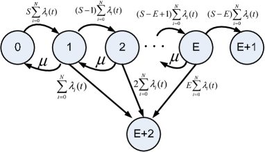
Figure 3: State transition after truncation.

To compute the system state after states truncation, we denote the new CTMC by $\{\bar{X}(t),t\geq 0\}$, the new generator matrix during period $(kT,(k+1)T)$ by $\bar{\boldsymbol{Q}}_{k}$, and the system state at time $(k+1)T$ by $\bar{\boldsymbol{\pi}}((k+1)T)$. We use notations with a bar to represent the case when system states of the CTMC are truncated if the context is clear. Similar to Equation (12), given the initial state $\bar{\boldsymbol{\pi}}(kT)$, the system state at time $(k+1)T$ for the CTMC $\{\bar{X}(t),t\geq 0\}$ can be derived as follows.

$$\bar{\boldsymbol{\pi}}((k+1)T)=\bar{\boldsymbol{\pi}}(kT)\sum_{n=0}^{\infty}\frac{(\bar{\boldsymbol{Q}}_{k}T)^{n}}{n!}.$$ (16)

If we denote the error caused by truncating the states at time $kT$ by $\bar{\epsilon}_{k}$, then $\bar{\epsilon}_{k}$ can be formally defined as follows.

$$\bar{\epsilon}_{k}=\max_{0\leq i\leq E}|\bar{\pi}_{i}(kT)-\pi_{i}(kT)|,$$

where $\bar{\pi}_{i}(kT)$ represents the probability of system being at state $i$ at time $kT$ for the CTMC $\{\bar{X}(t),t\geq 0\}$, i.e., the Markov chain after states truncation, and $\pi_{i}(kT)$ represents the probability of the system being at state $i$ at time $kT$ for the original CTMC $\{X(t),t\geq 0\}$. Clearly, $\bar{\epsilon}_{0}=0$ as the two Markov chains have the same initial states, i.e., $\bar{\pi}_{i}(0)=\pi_{i}(0)$. The bound of the error caused by states truncation is

$$\bar{\epsilon}_{k}\leq\bar{\pi}_{E+1}(kT).$$ (17)

Again, we can also follow the steps in Section III-A, i.e., use Algorithm 1, to compute the system state for the Markov chain after states truncation $\{\bar{X}(t),t\!\geq\!0\}$.

IV Model Validation

In this section, we validate via trace-driven simulation the accuracy of our CTMC model on quantifying the RAID reliability $R(t)$. We use the Microsoft’s SSD simulator [1] based on DiskSim [3]. Since each SSD contains multiple chips that can be configured to be independent of each other and handle I/O requests in parallel, we consider RAID at the chip level (as opposed to device level) in our DiskSim simulation. Specifically, we configure each chip to have its own data bus and control bus and treat it as one drive, and also treat the SSD controller as the RAID controller where parity-based RAID is built.

To simulate error arrivals, we generate error events based on Poisson arrivals given the current system age $k$ of the array. As the array ages, we update the error arrival rates accordingly by varying the variable $k_{i}(t)$ in Equation (7). We also generate recovery events whose recovery times follow an exponential distribution with a fixed rate $\mu=1$. Both error and recovery events are fed into the SSD simulator as special types of I/O requests. We consider three cases: error dominant, comparable, and recovery dominant, in which the error rate is larger than, comparable to, and smaller than the recovery rate, respectively.

Our validation measures the reliability of the traditional RAID and Diff-RAID with different parity distributions. Recall that Diff-RAID redistributes the parities after each drive replacement, while traditional RAID does not. We consider ($N+1$) chips where $N=3,5,7$. For traditional RAID, we choose RAID-5, in which parity chunks are evenly placed across the chips; for Diff-RAID, 10% of parity chunks placed in each of the $N$ chips and the remaining parity chunks are placed in the last flash chip.

We generate synthetic uniform workload in which the write requests access the addresses of the entire address space with equal probability. The workload lasts until all drives are worn out and replaced at least once. We run the DiskSim simulation 1000 times, and in each run we record the age when data loss happens. Finally, we derive the probability of data loss and the reliability based on our definitions. To speed up our DiskSim simulation, we consider a small-scale RAID array, in which each chip contains 80 blocks with 64 pages each, and the chunk size is set to be the same as the page size 4KB. We also set a low erasure limit at $M=100$ cycles for each block.

Figure 4 shows the reliability $R(t)$ versus the system age $k$ obtained from both the model and DiskSim results. We observe that our model accurately quantifies the reliability for all cases. Also, Diff-RAID shows its benefit only in the comparable case. In the error dominant case, traditional RAID always shows higher reliability than Diff-RAID; in the recovery dominant case, there is no significant difference between traditional RAID and Diff-RAID. We will further discuss these findings in Section V.

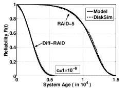
(a) Error dominant case (3+1 RAID)

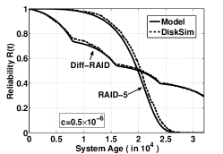
(b) Comparable case (3+1 RAID)

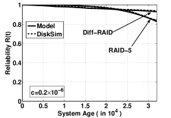
(c) Recovery dominant case (3+1 RAID)

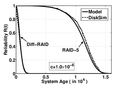
(d) Error dominant case (5+1 RAID)

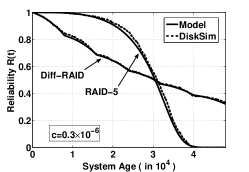
(e) Comparable case (5+1 RAID)

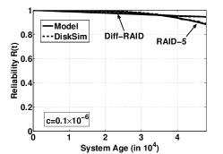
(f) Recovery dominant case (5+1 RAID)

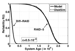
(g) Error dominant case (7+1 RAID)

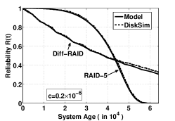
(h) Comparable case (7+1 RAID)

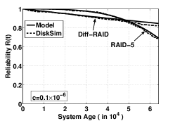
(i) Recovery dominant case (7+1 RAID)

Figure 4: Model validation with respect to different values of $N$ and different error rates.

V Numerical Analysis

In this section, we conduct numerical analysis on the reliability dynamics of a large-scale SSD RAID array with respect to different parity placement strategies. To this end, we summarize the lessons learned from our analysis.

V-A Choices of Default Model Parameters

We first describe the default model parameters used in our analysis, and provide justifications for our choices.

We consider an SSD RAID array composed of $N+1$ SSDs, each being modeled by the same set of parameters. By default, we set $N=9$. Each block of an SSD has 64 pages of size 4KB each. We consider 32GB SSDs with $B=131,072$ blocks. We configure the chunk size equal to the block size, i.e., there are $S=B=131,072$ chunks. We also have each block sustain $M=$10K erase cycles.

We now describe how we configure the error arrival rate, i.e., $\lambda_{i}=2ck_{i}$, by setting the constant $c$. We employ 4-bit ECC protection per 512 bytes of data, the industry standard for today’s MLC flash. Based on the uncorrectable bit error rates (UBERs) calculated in [2], we choose the UBER in the range $[10^{-16},10^{-18}]$ when an SSD reaches its rated lifetime (i.e., the erasure limit $M$ is reached). Since we set the chunk size to be equal to the block size, the probability that a chunk contains at least one bit error is roughly in the range of $[2\times 10^{-10},2\times 10^{-12}]$. Based on the analysis on real enterprise workload traces [29], an RAID array can have several hundred gigabytes of data being accessed per day. If the write request rate is set as 1TB per day (i.e., 50 blocks per second), then the error arrival rate per chunk at its rated lifetime (i.e., $\lambda_{i}=2cM$) is approximately in the range $[10^{-8},10^{-10}]$. The corresponding parameter $c$ is in the range $[0.5\times 10^{-12},0.5\times 10^{-14}]$.

For the error recovery rate $\mu$, we note that the aggregate error arrival rate when all $N+1$ drives are going to die out is $2cMS(N+1)$. If $N=9$, then the aggregate error arrival rate is roughly in the range $[10^{-2},10^{-4}]$. We fix $\mu=10^{-3}$.

We compare different cases when the error arrivals are more dominant than error recoveries, and vice versa. We consider three cases of error patterns: $c=1.1\times 10^{-13}$, $c=0.4\times 10^{-13}$, and $c=0.1\times 10^{-13}$, which correspond to the error dominant, comparable, and recovery dominant cases, respectively. Specifically, when $c=0.4\times 10^{-13}$, the aggregate error arrival rate of the array when all SSDs reach their rated lifetime is around $2cMS(N+1)\approx 10^{-3}$ (where $N=9$, $M=$10K, and $S=131,072$).

We now configure $T$, the time interval between two neighboring erase operations. Suppose that there are 1TB of writes per day as described above. The inter-arrival time of write requests is around $3\times 10^{-4}$ seconds for 4KB page size. Thus, the average time between two erase operations is $1.9\times 10^{-2}$ seconds as an erase is triggered after writing 64 pages. In practice, each erase causes additional writes (i.e., write amplification [15]) as it moves data across blocks, so $T$ should be smaller. Here, we fix $T=10^{-2}$ seconds.

We compare the reliability dynamics of RAID-5 and different variants of Diff-RAID. For RAID-5, each drive holds a fraction $\frac{1}{N+1}$ of parity chunks; for Diff-RAID, we choose the parity distribution (i.e., $p_{i}$’s for $0\leq i\leq N$) based on a truncated normal distribution. Specifically, we consider a normal distribution $\mathcal{N}(N+1,\sigma^{2})$ with mean $N+1$, and standard deviation $\sigma$, and let $f$ be the corresponding probability density function. We then choose $p_{i}$’s as follows:

$$p_{i}=\frac{\int_{i}^{i+1}f(x)dx}{\int_{0}^{N+1}f(x)dx},\quad 0\leq i\leq N.$$ (18)

We can choose different distributions of $p_{i}$ by tuning the parameter $\sigma$. Intuitively, the larger $\sigma$ is, the more evenly $p_{i}$’s are distributed. We consider three cases: $\sigma=1$, $\sigma=2$, and $\sigma=5$. Suppose that $N=9$. Then for $\sigma=1$, SSD $N$ and SSD $N-1$ hold 68% and 27% of parity chunks, respectively; for $\sigma=2$, SSD $N$, SSD $N-1$, and SSD $N-2$ hold 38%, 30%, and 18% of parity chunks, respectively; for $\sigma=5$, the proportions of parity chunks range from 2.8% (in SSD 0) to 16.6% (in SSD $N$). After choosing $p_{i}$’s, the age of each block of SSD $i$ (i.e., $k_{i}$) can be computed via Equation (5).

V-B Impact of Different Error Dynamics

We now show the numerical results of RAID reliability based on the parameters described earlier. We assume that drive replacement can be completed immediately after the oldest SSD reaches its rated lifetime. When the oldest drive is replaced, all its chunks (including any erroneous chunks) are copied to the new drive. Thus, the reliability (or the probability of no data loss) remains the same. We consider three error cases: error dominant, comparable, and recovery dominant cases, as described above.

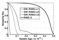
(a) Error dominant case ($c=1.1\times 10^{-13}$)

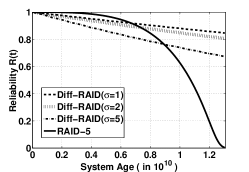
(b) Comparable case ($c=0.4\times 10^{-13}$)

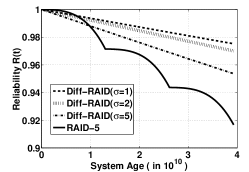
(c) Recovery dominant case ($c=0.1\times 10^{-13}$)

Figure 5: Reliability dynamics of SSD arrays.

Case 1: Error dominant case. Figure 5(a) first shows the numerical results for the error dominant case. Initially, RAID-5 achieves very good reliability as all drives are brand-new. However, as SSDs wear down, the bit error rate increases, and this makes the RAID reliability decrease very quickly. In particular, the reliability drops to zero (i.e., data loss always happen) when the array performs around $5\times 10^{9}$ erasures. For Diff-RAID, the more evenly parity chunks are distributed, the lower RAID reliability is. In the error dominant case, since error arrival rate is much bigger than the recovery rate, the RAID reliability drops to zero very quickly no matter what parity placement strategy is used. We note that Diff-RAID is less reliable than traditional RAID-5 in the error dominant case. The reason is that for Diff-RAID, the initial ages of SSDs when constructing the RAID array are non-zero, but instead follow the convergent age distribution (i.e., based on $A_{i}$’s in Equation (3)). When error arrival rate is very large, the array suffers from low reliability even if the array only performs small number of erasures. However, for RAID-5, since it is always constructed by using brand-new SSDs, it starts with a very high reliability.

Case 2: Comparable case. Figure 5(b) shows the results for the comparable case. RAID-5 achieves very good reliability initially, but decreases dramatically as the SSDs wear down. Also, all drives wear down at the same rate, the reliability of the array is about zero when all drives reach their erasure limits, i.e., when the system age is around $1.3\times 10^{10}$ erasures. Diff-RAID shows different reliability dynamics. Initially, Diff-RAID has less reliability than RAID-5, but the drop rate of the reliability is much slower than that of RAID-5 as SSDs wear down. The reason is that Diff-RAID has uneven parity placement, SSDs are worn out at different times and will be replaced one by one. When the worn-out SSD is replaced, other SSDs perform fewer erase operations and have small error rates. This prevents the whole array suffering from a very large error rate as in RAID-5. Also, the reliability is higher when the parity distribution is more skewed (i.e., smaller $\sigma$), as also observed in [2].

Case 3: Recovery dominant case. Figure 5(c) shows the results for the recovery dominant case. RAID-5 shows high reliability in general. Between two replacements (which happens every $1.3\times 10^{10}$ erasures), its data loss probability drops by within 3%. Its reliability drops slowly right after each replacement, and its drop rate increases as it is close to be worn out. Diff-RAID shows higher reliability than RAID-5 in general, but the difference is small (e.g., less than 6% between Diff-RAID for $\sigma=1$ and RAID-5). Therefore, in the recovery dominant scenario, we may deploy RAID-5 instead of Diff-RAID, as the latter introduces higher costs in parity redistribution in each replacement and has smaller I/O throughput due to load imbalance of parities.

V-C Impact of Different Array Configurations

We further study via our model how different array configurations affect the RAID reliability. We focus on Diff-RAID and generate the parity distribution $p_{i}$’s with $\sigma=1$. Our goal is to validate the robustness of our model on characterizing the reliability for different array configurations.

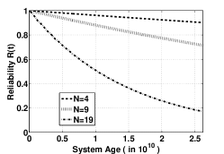
(a) Impact of $N$

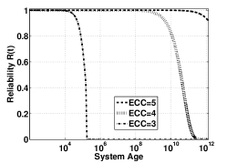
(b) Impact of ECC length

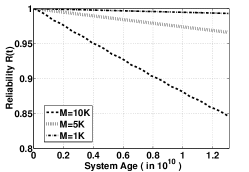
(c) Impact of $M$

Figure 6: Impact of different RAID configurations on the reliability.

Impact of $N$. Figure 6(a) shows the impact of the RAID size $N$. We fix other parameters as the same in the comparable case, i.e., $\mu=10^{-3}$, $c=0.4\times 10^{-13}$, and $M=10^{4}$. The larger the system size, the lower the RAID reliability. Intuitively, the probability of having one more erroneous chunk in a stripe increases with the stripe width (i.e., $N+1$). Note that the reliability drop is significant when $N$ increases. For example, at $2.6\times 10^{10}$ erasures, the reliability drops from 0.7 to 0.2 when $N$ increases from 9 to 19.

Impact of ECC. Figure 6(b) shows the impact of different ECC lengths. We fix $\mu=10^{-3}$, $M=10^{4}$, and $N=9$. We also fix the raw bit error rate (RBER) as $1.3\times 10^{-6}$ [2], and compute the uncorrectable bit error rate using the formulas in [27]. Then as described in Section V-A, we derive $c$ for different ECCs that can correct 3, 4, 5 bits per 512 byte sector, and the corresponding values are $4.4\times 10^{-11}$, $4.7\times 10^{-14}$, and $4.2\times 10^{-17}$, respectively. We observe that the RAID reliability drops to zero very quickly for 3-bit ECC at around $10^{5}$ erasures, while the RAID reliability for 5-bit ECC starts to decrease until the array performs $10^{11}$ erasures. This shows that the RAID reliability heavily depends on the reliability of each single SSD, or the ECC length employed in each SSD.

Impact of $M$. Figure 6(c) shows the impact of the erasure limit $M$, or the endurance of a single SSD, on the RAID reliability. We fix other parameters with $\mu=10^{-3}$, $N=9$ and $c=0.4\times 10^{-13}$. We observe that when $M$ decreases, the RAID reliability increases. For example, at $1.3\times 10^{10}$ erasures, the RAID reliability increases from 0.85 to 0.99 when $M$ decreases from 10K to 1K. Recall that the error rates increase with the number of erasures in SSDs. We now have the increase of bit error rates capped by the small erasure limit. The trade-off is that the SSDs are worn out and replaced more frequently with smaller $M$.

V-D Discussion

Our results provide several insights into constructing RAID for SSDs.

• The error dominant case may correspond to the low-end MLC or TLC SSDs with high bit error rates, especially when these types of SSDs have low I/O bandwidth for RAID reconstruction. Both traditional RAID-5 and Diff-RAID show low reliability. A higher degree of fault tolerance (e.g., using RAID-6 or stronger ECC) becomes necessary in this case.

• When the error arrival and recovery rates are similar, Diff-RAID, with uneven parity distribution, achieves higher reliability than RAID-5, especially when RAID-5 reaches zero reliability when all SSDs are worn out simultaneously. This conforms to the findings in [2].

• In the recovery dominant case, which may correspond to the high-end single-level cell (SLC) SSDs that typically have very small bit error rates, RAID-5 achieves very high reliability. We may choose RAID-5 over Diff-RAID in RAID deployment to save the overhead of parity redistribution in Diff-RAID.

• Our model can effectively analyze the RAID reliability with regard to different RAID configurations.

VI Related Work

There have been extensive studies on NAND flash-based SSDs. A detailed survey of the algorithms and data structures for flash memories is found in [11]. Recent papers empirically study the intrinsic characteristics of SSDs (e.g., [1, 5]), or develop analytical models for the write performance (e.g., [9, 15]) and garbage collection algorithms (e.g., [23]) of SSDs.

Bit error rates of SSDs are known to increase with the number of erase cycles [27, 12]. To improve reliability, prior studies propose to adopt RAID for SSDs at the device level [2, 16, 21, 22, 30, 25], or at the chip level [20]. These studies focus on developing new RAID schemes that improve the performance and endurance of SSDs over traditional RAID. The performance and reliability implications of RAID on SSDs are also experimentally studied in [19]. In contrast, our work focuses on quantifying reliability dynamics of SSD RAID from a theoretical perspective. Authors of Diff-RAID [2] also attempt to quantify the reliability, but they only compute the reliability at the instants of SSD replacements, while our model captures the time-varying nature of error rates in SSDs and quantifies the instantaneous reliability during the whole lifespan of an SSD RAID array.

RAID was first introduced in [31] and has been widely used in many storage systems. Performance and reliability analysis on RAID in the context of hard disk drives has been extensively studied (e.g., see [28, 6, 4, 24, 35]). On the other hand, SSDs have a distinct property that their error rates increase as they wear down, so a new model is necessary to characterize the reliability of SSD RAID.

VII Conclusions

We develop the first analytical model that quantifies the reliability dynamics of SSD RAID arrays. We build our model as a non-homogeneous continuous time Markov chain, and use uniformization to analyze the transient state of the RAID reliability. We validate the correctness of our model via trace-driven DiskSim simulation with SSD extensions.

One major application of our model is to characterize the reliability dynamics of general RAID schemes with different parity placement distributions. To demonstrate, we compare the reliability dynamics of the traditional RAID-5 scheme and the new Diff-RAID scheme under different error patterns and different array configurations. Our model provides a useful tool for system designers to understand the reliability of an SSD RAID array with regard to different scenarios.

-A Proof of Theorem 1 in Section III-A

The computation of the system state in Equation (14) is intuitive since the truncation point is $U_{l}$ in interval $(lsT,(l+1)sT)$. In the following, we focus on the derivation of the error bound. Note that $\boldsymbol{\pi}((l+1)sT)$ is the system state at time $(l+1)sT$ for the CTMC $\{X(t)\}$. Moreover, given the state at time $lsT$, $\boldsymbol{\pi}((l+1)sT)$ is computed iteratively by computing $\boldsymbol{\pi}((ls+1)T)$, $\boldsymbol{\pi}((ls+2)T)$, …, $\boldsymbol{\pi}((ls+s)T)$ sequentially. During each step, e.g., deriving $\boldsymbol{\pi}((k+1)T)$ from $\boldsymbol{\pi}(kT)$ ($ls\leq k<(l+1)s$), uniformization is used. Without loss of generality, we can let $\Lambda_{k}=\tilde{\Lambda}_{l}$ ($ls\leq k<(l+1)s$) as $\tilde{\Lambda}_{l}\geq\max_{0\leq i\leq S+1}|-q_{i,i}(k)|$ for all $k$ ($ls\leq k<(l+1)s$). Since $\boldsymbol{Q}_{k}$ is denoted as the generator matrix of the homogeneous CTMC $\{X(t),kT<t\leq(k+1)T\}$, to apply the uniformization, we let $\boldsymbol{P}_{k}=\boldsymbol{I}+\frac{\boldsymbol{Q}_{k}}{\tilde{\Lambda}_{l}}$ ($ls\leq k<(l+1)s$). Since every element of $\boldsymbol{P}_{k}$ is a linear function of $k$, the difference between two matrices $\boldsymbol{P}_{k+1}-\boldsymbol{P}_{k}$ must be the same for all $k$, and we denote it by $\boldsymbol{D}$. Formally, we have

$$\boldsymbol{D}=\boldsymbol{P}_{k+1}-\boldsymbol{P}_{k},\;ls\leq k<(l+1)s$$ (19)

Now, we can easily find that $\boldsymbol{P}_{k}=\boldsymbol{P}_{ls}+(k-ls)\boldsymbol{D}$ ($ls\leq k\leq(l+1)s-1$). Moreover, since $\tilde{\boldsymbol{P}_{l}}=\boldsymbol{I}+\frac{\tilde{\boldsymbol{Q}}_{l}}{\tilde{\Lambda}_{l}}$ and $\tilde{\boldsymbol{Q}}_{l}$ is defined as $\frac{\sum_{k=ls}^{(l+1)s-1}\boldsymbol{Q}_{k}}{s}$ in Equation (11), we have

$$\tilde{\boldsymbol{P}_{l}} = \frac{\sum_{k=ls}^{(l+1)s-1}\boldsymbol{P}_{k}}{s}=\frac{\sum_{k=ls}^{(l+1)s-1}(\boldsymbol{P}_{ls}+(k-ls)\boldsymbol{D})}{s}$$ (20)

$$= \boldsymbol{P}_{ls}+\frac{s-1}{2}\boldsymbol{D}.$$

Note that based on the analysis of $\{X(t),kT<t\leq(k+1)T\}$ by using uniformization, $\boldsymbol{\pi}((k+1)T)$ ($ls\leq k<(l+1)s$) can be rewritten as follows.

$$\boldsymbol{\pi}((k+1)T) = \boldsymbol{\pi}(kT)e^{-\tilde{\Lambda}_{l}T}e^{\tilde{\Lambda}_{l}T\boldsymbol{P}_{k}}$$

$$= \boldsymbol{\pi}(kT)e^{-\tilde{\Lambda}_{l}T}e^{\tilde{\Lambda}_{l}T(\boldsymbol{P}_{ls}+(k-ls)\boldsymbol{D})}.$$

Observe that most elements in the difference matrix $\boldsymbol{D}$ are zero, and the non-zero elements are all very small, by examining the elements in $\boldsymbol{D}\boldsymbol{P}_{ls}$ and the elements in $\boldsymbol{P}_{ls}\boldsymbol{D}$, we find that the multiplication of matrix $\boldsymbol{D}$ and matrix $\boldsymbol{P}_{ls}$ can be assumed to be commutative, or $\boldsymbol{D}\boldsymbol{P}_{ls}\approx\boldsymbol{P}_{ls}\boldsymbol{D}$. Therefore, we have

$$\boldsymbol{\pi}((l+1)sT) \approx \boldsymbol{\pi}(lsT)e^{-\tilde{\Lambda}_{l}sT}e^{\tilde{\Lambda}_{l}T\sum_{k=ls}^{(l+1)s-1}\boldsymbol{P}_{k}}$$

$$= \boldsymbol{\pi}(lsT)e^{-\tilde{\Lambda}_{l}sT}e^{\tilde{\Lambda}_{l}Ts\tilde{\boldsymbol{P}}_{l}}.$$

Now, the upper bound of the error $\hat{\tilde{\epsilon}}_{l}$ is derived as follows.

$$\hat{\tilde{\epsilon}}_{l}\!\!\!\!\!\! = \!\!\!\!\!\!||\hat{\tilde{\boldsymbol{\pi}}}((l+1)sT)-\boldsymbol{\pi}((l+1)sT)||_{1}$$

$$= \!\!\!\!\!\!||\hat{\tilde{\boldsymbol{\pi}}}(lsT)\!\!\!\sum_{n=0}^{U_{l}}\!\!e^{\!-\!\tilde{\Lambda}_{l}sT}\!\frac{(\tilde{\Lambda}_{l}sT)^{n}}{n!}\!\tilde{\boldsymbol{P}}_{l}^{n}\!\!\!-\!\!\boldsymbol{\pi}(lsT)e^{\!-\!\tilde{\Lambda}_{l}sT}e^{\tilde{\Lambda}_{l}Ts\tilde{\boldsymbol{P}}_{l}}\!||_{1}$$

$$\leq \!\!\!\!\!\!||\hat{\tilde{\boldsymbol{\pi}}}(lsT)e^{-\tilde{\Lambda}_{l}sT}e^{\tilde{\Lambda}_{l}sT\tilde{\boldsymbol{P}}_{l}}\!-\!\boldsymbol{\pi}(lsT)e^{-\tilde{\Lambda}_{l}sT}e^{\tilde{\Lambda}_{l}Ts\tilde{\boldsymbol{P}}_{l}}||_{1}$$

$$+||\hat{\tilde{\boldsymbol{\pi}}}(lsT)\!\!\sum_{n=U_{l}+1}^{\infty}\!\!e^{-\tilde{\Lambda}_{l}sT}\frac{(\tilde{\Lambda}_{l}sT)^{n}}{n!}\tilde{\boldsymbol{P}}_{l}^{n}||_{1}$$

$$\leq \!\!\!\!\!\!||\hat{\tilde{\boldsymbol{\pi}}}(lsT)-\boldsymbol{\pi}(lsT)||_{1}e^{-\tilde{\Lambda}_{l}sT}e^{\tilde{\Lambda}_{l}sT||\tilde{\boldsymbol{P}}_{l}||_{\infty}}$$

$$+\left(1-\sum_{n=0}^{U_{l}}e^{-\tilde{\Lambda}_{l}sT}\frac{(\tilde{\Lambda}_{l}sT)^{n}}{n!}\right)$$

$$= \!\!\!\!\!\!\hat{\tilde{\epsilon}}_{l-1}+\left(1-\sum_{n=0}^{U_{l}}e^{-\tilde{\Lambda}_{l}sT}\frac{(\tilde{\Lambda}_{l}sT)^{n}}{n!}\right).$$

The last equation comes from the fact that $||\tilde{\boldsymbol{P}}_{l}||_{\infty}=1$ as $\tilde{\boldsymbol{P}}_{l}=\boldsymbol{I}+\frac{\tilde{\boldsymbol{Q}}_{l}}{\tilde{\Lambda}_{l}}$, and $\hat{\tilde{\epsilon}}_{l-1}=||\hat{\tilde{\boldsymbol{\pi}}}(lsT)-\boldsymbol{\pi}(lsT)||_{1}$. Therefore, we have the results stated in Theorem 1.

References

- [1] N. Agrawal, V. Prabhakaran, T. Wobber, J. D. Davis, M. Manasse, and R. Panigrahy. Design Tradeoffs for SSD Performance. In Proc. of USENIX ATC, Jun 2008.
- [2] M. Balakrishnan, A. Kadav, V. Prabhakaran, and D. Malkhi. Differential RAID: Rethinking RAID for SSD Reliability. ACM Trans. on Storage, 6(2):4, Jul 2010.
- [3] J. S. Bucy, J. Schindler, S. W. Schlosser, and G. R. Ganger. The DiskSim Simulation Environment Version 4.0 Reference Manual. Technical Report CMUPDL-08-101, May 2008.
- [4] W. Burkhard and J. Menon. Disk Array Storage System Reliability. In Proc. of IEEE FTCS, Jun 1993.
- [5] F. Chen, D. A. Koufaty, and X. Zhang. Understanding Intrinsic Characteristics and System Implications of Flash Memory Based Solid State Drives. In SIGMETRICS, 2009.
- [6] S. Chen and D. Towsley. A Performance Evaluation of RAID Architectures. IEEE T. on Comp., 45(10):1116–1130, 1996.
- [7] E. de Souza e Silva and H. R. Gail. Transient Solutions for Markov Chains. Computational Probability, W. K. Grassmann (editor). Kluwer Academic Publishers:43–81, 2000.
- [8] E. Deal. Trends in NAND Flash Memory Error Correction. http://www.cyclicdesign.com/whitepapers/Cyclic_Design_NAND_ECC.pdf, Jun 2009.
- [9] P. Desnoyers. Analytic Modeling of SSD Write Performance. In Proc. of SYSTOR, Jun 2012.
- [10] R. Enderle. Revolution in January: EMC Brings Flash Drives into the Data Center. http://www.itbusinessedge.com/blogs/rob/?p=184, Jan 2008.
- [11] E. Gal and S. Toledo. Algorithms and Data Structures for Flash Memories. ACM Comput. Surv., 37(2):138–163, 2005.
- [12] L. M. Grupp, A. M. Caulfield, J. Coburn, S. Swanson, E. Yaakobi, P. H. Siegel, and J. K. Wolf. Characterizing Flash Memory: Anomalies, Observations, and Applications. In Proc. of IEEE/ACM MICRO, Dec 2009.
- [13] L. M. Grupp, J. D. Davis, and S. Swanson. The Bleak Future of NAND Flash Memory. In USENIX FAST, Feb 2012.
- [14] K. Hess. 2011: Year of the SSD? http://www.datacenterknowledge.com/archives/2011/02/17/2011-year-of-the-ssd/, Feb 2011.
- [15] X.-Y. Hu, E. Eleftheriou, R. Haas, I. Iliadis, and R. Pletka. Write Amplification Analysis in Flash-based Solid State Drives. In Proc. of SYSTOR, May 2009.
- [16] S. Im and D. Shin. Flash-Aware RAID Techniques for Dependable and High-Performance Flash Memory SSD. IEEE Trans. on Computers, 60:80–92, Jan 2011.
- [17] Intel. Intel Solid-State Drive 710: Endurance. Performance. Protection. http://www.intel.com/content/www/us/en/solid-state-drives/solid-state-drives-710-series.html.
- [18] A. Jensen. Markoff Chains As An Aid in The Study of Markoff Processes. Scandinavian Actuarial Journal, 3:87–91, 1953.
- [19] N. Jeremic, G. Mühl, A. Busse, and J. Richling. The Pitfalls of Deploying Solid-state Drive RAIDs. In SYSTOR, 2011.
- [20] J. Kim, J. Lee, J. Choi, D. Lee, and S. H. Noh. Enhancing SSD Reliability Through Efficient RAID Support. In Proc. of APSys, Jul 2012.
- [21] S. Lee, B. Lee, K. Koh, and H. Bahn. A Lifespan-aware Reliability Scheme for RAID-based Flash Storage. In Proc. of ACM Symp. on Applied Computing, SAC ’11, 2011.
- [22] Y. Lee, S. Jung, and Y. H. Song. FRA: A Flash-aware Redundancy Array of Flash Storage Devices. In Proc. of ACM CODES+ISSS, Oct 2009.
- [23] Y. Li, P. P. C. Lee, and J. C. S. Lui. Stochastic Modeling of Large-Scale Solid-State Storage Systems: Analysis, Design Tradeoffs and Optimization. In Proc. of SIGMETRICS, 2013.
- [24] M. Malhotra and K. S. Trivedi. Reliability Analysis of Redundant Arrays of Inexpensive Disks. J. Parallel Distrib. Comput., 17(1-2):146–151, Jan 1993.
- [25] B. Mao, H. Jiang, S. Wu, L. Tian, D. Feng, J. Chen, and L. Zeng. HPDA: A Hybrid Parity-based Disk Array for Enhanced Performance and Reliability. ACM Trans. on Storage, 8(1):4, Feb 2012.
- [26] M. Mariano. ECC Options for Improving NAND Flash Memory Reliability. http://www.micron.com/~/media/Documents/Products/Software%20Article/SWNL_implementing_ecc.pdf, Nov 2011.
- [27] N. Mielke, T. Marquart, N. Wu, J. Kessenich, H. Belgal, E. Schares, F. Trivedi, E. Goodness, and L. Nevill. Bit Error Rate in NAND Flash Memories. In IEEE Int. Reliability Physics Symp., Apr 2008.
- [28] R. R. Muntz and J. C. S. Lui. Performance Analysis of Disk Arrays under Failure. In Proc. of VLDB, Aug 1990.
- [29] D. Narayanan, E. Thereska, A. Donnelly, S. Elnikety, and A. Rowstron. Migrating Server Storage to SSDs: Analysis of Tradeoffs. In Proc. of ACM EuroSys, Mar 2009.
- [30] K. Park, D.-H. Lee, Y. Woo, G. Lee, J.-H. Lee, and D.-H. Kim. Reliability and Performance Enhancement Technique for SSD Array Storage System Using RAID Mechanism. In IEEE Int. Symp. on Comm. and Inform. Tech., 2009.
- [31] D. A. Patterson, G. Gibson, and R. H. Katz. A Case for Redundant Arrays of Inexpensive Disks (RAID). In Proc. of ACM SIGMOD, Jun 1988.
- [32] A. Reibman and K. S. Trivedi. Transient Analysis of Cumulative Measures of Markov Model Behavior. Communications in Statistics-Stochastic Models, 5:683–710, 1989.
- [33] M. Schulze, G. Gibson, R. Katz, and D. Patterson. How Reliable Is A RAID? In IEEE Computer Society International Conference: Intellectual Leverage, Digest of Papers, 1989.
- [34] W. Weibull. A Statistical Distribution Function of Wide Applicability. J. of Applied Mechanics, 18:293–297, 1951.
- [35] X. Wu, J. Li, and H. Kameda. Reliability Analysis of Disk Array Organizations by Considering Uncorrectable Bit Errors. In Proc. of IEEE SRDS, Oct 1997.