Improved Accuracy and Parallelism for MRRR-based Eigensolvers – A Mixed Precision Approach

Abstract

The real symmetric tridiagonal eigenproblem is of outstanding importance in numerical computations; it arises frequently as part of eigensolvers for standard and generalized dense Hermitian eigenproblems that are based on a reduction to tridiagonal form. For its solution, the algorithm of Multiple Relatively Robust Representations (MRRR) is among the fastest methods. Although fast, the solvers based on MRRR do not deliver the same accuracy as competing methods like Divide & Conquer or the QR algorithm. In this paper, we demonstrate that the use of mixed precisions leads to improved accuracy of MRRR-based eigensolvers with limited or no performance penalty. As a result, we obtain eigensolvers that are not only equally or more accurate than the best available methods, but also – under most circumstances – faster and more scalable than the competition.

1 Introduction

In [21], the authors describe how in libraries the use of “higher internal precision and mixed input/output types and precisions permits […] to implement some algorithms that are simpler, more accurate, and sometimes faster.” In particular, the internal use of higher precision provides the library developer with extra precision and a wider range of values, which may benefit the accuracy and robustness of numerical routines. In sharp contrast to software that uses arbitrary precision to obtain any desired accuracy, the use of higher precision should not lower performance significantly if at all. In this paper, we employ mixed precisions to improve not only the accuracy, but also the robustness and scalability of eigensolvers based on the algorithm of Multiple Relatively Robust Representations (MRRR or MR³ for short) [12, 3, 36, 31, 32, 37].

Direct methods for standard and generalized Hermitian eigenproblems often rely on a reduction to real symmetric tridiagonal form [5]. Once the problem is transformed, the real symmetric tridiagonal eigenproblem (STEP) is the following: Given a tridiagonal matrix $T\in\mathbb{R}^{n\times n}$ (with $T=T^{*}$, where $T^{*}$ denotes the transpose of $T$), find quantities $\lambda\in\mathbb{R}$ and nonzero $z\in\mathbb{R}^{n}$ such that the equation

$$Tz=\lambda z$$

holds. Without loss of generality, we assume $\lVert z\rVert=1$ hereafter, where $\lVert\bullet\rVert$ denotes the 2-norm. For such a solution, $\lambda$ is called an eigenvalue (of $T$) and $z$ an associated eigenvector; an eigenvalue together with an associated eigenvector are said to form an eigenpair, $(\lambda,z)$. The Spectral Theorem [24] ensures the existence of $n$ eigenpairs $(\lambda_{i},z_{i})$, $i\in\{1,2,\ldots,n\}$, such that the eigenvectors form a complete orthonormal set; that is, for all $i,j\in\{1,2,\ldots,n\}$,

$$z_{j}^{*}z_{i}=\left\{\begin{array}[]{l l}1&\quad\text{if $j=i$}\,,\\ 0&\quad\text{if $j\neq i$}\,.\\ \end{array}\right.$$

Since all eigenvalues are real, they can be ordered:

$$\lambda_{1}\leq\lambda_{2}\leq\ldots\leq\lambda_{i}\leq\ldots\leq\lambda_{n}\,,$$

where $\lambda_{i}$ is the $i$-th smallest eigenvalue of $T$. In this paper, whenever the underlying matrix is not clear, we write $\lambda_{i}[T]$ explicitly. The set of all eigenvalues of $T$ is denoted $spec[T]$ and the spectral diameter is defined as $spdiam[T]=\lambda_{n}-\lambda_{1}$. For a given index set $\mathcal{I}\subseteq\{1,2,\ldots,n\}$,

$$\mathcal{Z}_{\mathcal{I}}=\mbox{span}\{z_{i}:i\in\mathcal{I}\}$$

denotes the invariant subspace associated with $\mathcal{I}$. As with the eigenvalues, whenever the underlying matrix is not understood from context, we write $\mathcal{Z}_{\mathcal{I}}[T]$ explicitly.

In many applications, only a subset of eigenpairs are of interest and need to be computed. For the computed eigenpairs, $(\hat{\lambda}_{i},\hat{z}_{i})$, $\lVert\hat{z}_{i}\rVert=1$ and $i\in\mathcal{I}\subseteq\{1,2,\ldots,n\}$, the accuracy of the results can be quantified by the largest residual norm and the orthogonality, respectively defined as

$$R=\max_{i\in\mathcal{I}}\frac{\|T\hat{z}_{i}-\hat{\lambda}_{i}\hat{z}_{i}\|_{1}}{\|T\|_{1}}\quad\mbox{and}\quad O=\max_{i\in\mathcal{I}}\max_{\begin{subarray}{c}j\in\mathcal{I}\\ j\neq i\end{subarray}}|\hat{z}_{j}^{*}\hat{z}_{i}|\,.$$ (1)

A number of excellent algorithms for the STEP have been discovered. Among them, Bisection and Inverse Iteration (BI) [8, 19], the QR algorithm (QR) [15, 20], Divide & Conquer (DC) [4, 16, 17], and the focus of this study, MRRR [7, 10, 9, 26, 27, 37]. These methods differ in various aspects: the number of floating point operations (flops) they perform, the flop-rate at which the operations are executed, the amount of memory required, the possibility of computing subsets of eigenpairs at reduced cost, the attainable accuracy, the simplicity and robustness of the code, and the suitability for parallel computations. Thus, the “best” algorithm is influenced by factors such as the problem (e.g., dimension, subset, spectral distribution), the architecture (e.g., cache sizes, parallelism), external libraries (e.g., Basic Linear Algebra Subprograms), and the specific implementation of the algorithm (e.g., thresholds, optimizations).

Demmel et al. [6] provide a detailed study of the performance and accuracy of LAPACK’s [1] implementations of these four methods on various architectures. They conclude that ($i$) DC and QR are the most accurate algorithms; ($ii$) DC requires $\mathcal{O}(n^{2})$ additional memory and therefore much more than all the other algorithms; ($iii$) DC and MRRR are much faster than QR and BI; despite the fact that MRRR uses the fewest flops, DC is faster on certain classes of matrices. If the full eigendecomposition is desired, DC is generally the method of choice, but whether DC or MRRR is faster depends on the spectral distribution of the input matrix; and ($iv$) if only a subset of eigenpairs is desired, MRRR is the method of choice. The study is limited to sequential executions and does not take into account the degree of parallelism the algorithms provide. However, various studies [3, 36, 32, 34, 31] of the performance and accuracy of parallel implementations come to similar conclusions.

To summarize, if all eigenpairs are computed, depending on the spectral distribution of the input matrix, either DC or MRRR is the fastest method. If only a subset of eigenpairs is desired, MRRR is the method of choice. Unfortunately, MRRR delivers generally the least accurate results. These observations carry over to direct methods for the dense eigenproblem based on a reduction to tridiagonal form. It is natural to ask whether the accuracy of the MRRR-based routines can be improved to levels of other methods like QR or DC. Unfortunately, a general analysis of any MRRR implementation shows that, even if all requirements of the algorithm are fulfilled, one needs to expect orthogonality of $\mathcal{O}(1000n\varepsilon)$ – with unit roundoff $\varepsilon$ [38]. Methods like QR and DC, however, attain superior results with orthogonality of $\mathcal{O}(\varepsilon\sqrt{n})$. In this paper, we present a practical solution that improves the accuracy of MRRR. As a result, it becomes equally or more accurate than QR and DC.

Our solution resorts to the use of higher precision arithmetic. The motivation is twofold: ($i$) MRRR is frequently the fastest algorithm and it might be possible to trade (some of) its performance to obtain higher accuracy; ($ii$) often MRRR is used in the context of direct methods for Hermitian eigenproblems. While the tridiagonal stage is responsible for much of the “loss” of orthogonality in the final result, it has a lower complexity than the reduction to tridiagonal form. Thus, even if it is necessary to spend more time in the tridiagonal stage to improve accuracy, for sufficiently large matrices, the overall run time will not be affected significantly. As MRRR does not make use of any level-3 Basic Linear Algebra Subprograms (BLAS) [13], we do not require in our mixed precision approach any optimized BLAS library for high precision, which might not be available.

For any MRRR solver, we present how the use of mixed precisions leads to more accurate results at very little or even no extra costs in terms of performance. As a consequence, MRRR is not only one of the fastest methods, but also becomes as accurate or even more accurate than the competition. Moreover, for direct methods based on a reduction to tridiagonal form and MRRR, the tridiagonal eigensolver is responsible for the inferior orthogonality compared with other methods. These solvers benefit directly from our approach.

1.1 Related work and outline

The term mixed precision algorithm is sometimes synonymously used for the following procedure: First solve the problem using a fast low-precision arithmetic, and then refine the result to high accuracy using a high-precision arithmetic. This mixed precision iterative refinement approach exploits the fact that there might exist a low-precision arithmetic faster than that of the input/output data format. The larger the performance gap between the two arithmetic, the more beneficial the approach. Iterative refinement (with and without using mixed precisions) has been most extensively studied for the solution of linear systems of equations [18], but other operations such as the solution of Lyapunov equations also benefit from it [2].

We use of the term mixed precision in its more general form; that is, using two or more different precisions for solving a problem. In particular, we use a higher precision in the more sensitive parts of an algorithm to obtain accuracy, which otherwise could not be achieved. This approach is especially effective if the sensitive portion of the algorithm and/or the performance gap between the two arithmetic is small. Similarly to the mixed precision ideas for iterative refinement, the approach is quite general and we believe it can benefit computations in numerous areas.

The rest of the paper is organized as follows: In Section 2, we present the MRRR algorithm and its accuracy limitations. The section mainly serves as a vehicle to introduce the factors that influence accuracy, which are summarized in Theorem 1. The derivation of the error bounds, which can be found in [38], is not important for the understanding of our discussion. In Section 3, we detail our mixed precision approach in a general setting. Besides presenting a way to improve accuracy, we investigate the effects on memory usage, robustness, and scalability. In Section 4, we comment on an actual implementation of our approach and elaborate on a number of practical issues. Finally, we present experimental results of our mixed precision solvers in Section 5.

2 The MRRR algorithm

In this section, we present the MRRR algorithm to the detail necessary for the later discussion. Our exposition is largely based on [38, 40, 9] and a high-level description of the method given in Algorithm 1. We comment more thoroughly on various parts of the computation in the following. The goal is to present Theorem 1 – i.e., the factors that influence the accuracy of any implementation of MRRR.

Preprocessing

Algorithm 1 assumes that the necessary preprocessing is already performed; this includes the scaling of the entries, and the so called splitting of the input matrix into principal submatrices if off-diagonal entries are sufficiently small in magnitude [24]. In this section, without any loss is generality, we assume that the input matrix is (numerically) irreducible, i.e., no off-diagonal entry is “small enough” in magnitude that warrants setting it to zero. The exact criterion is specified later.

Input: Irreducible symmetric tridiagonal $T\in\mathbb{R}^{n\times n}$; index set $\mathcal{I}_{in}\subseteq\{1,\ldots,n\}$.
Output: Eigenpairs $(\hat{\lambda}_{i},\hat{z}_{i})$ with $i\in\mathcal{I}_{in}$.

1:  Select shift $\mu\in\mathbb{R}$ and compute $M_{root}=T-\mu I$.

2:  Perturb $M_{root}$ by a “random” relative amount bounded by a small multiple of $\varepsilon$.

3:  Compute $\hat{\lambda}_{i}[M_{root}]$ with $i\in\mathcal{I}_{in}$ to relative accuracy sufficient for classification.

4:  Form a work queue $Q$ and enqueue task $\{M_{root},\mathcal{I}_{in},\mu\}$.

5:  while $Q$ not empty do

6:       Dequeue a task $\{M,\mathcal{I},\sigma\}$.

7:       Partition $\mathcal{I}=\bigcup_{r=1}^{R}\mathcal{I}_{r}$ according to the separation of the eigenvalues.

8:       for $r=1$ to $R$ do

9:             if $\mathcal{I}_{r}=\{i\}$ then

10:                  // process well-separated eigenvalue associated with singleton $\mathcal{I}_{r}$ //

11:                  Perform Rayleigh quotient iteration (guarded by bisection) to obtain eigenpair $(\hat{\lambda}_{i}[M],\hat{z}_{i})$ with sufficiently small residual norm, $\lVert M\hat{z}_{i}-\hat{\lambda}_{i}[M]\,\hat{z}_{i}\rVert$.

12:                  Return $\hat{\lambda}_{i}[T]=\hat{\lambda}_{i}[M]+\sigma$ and $\hat{z}_{i}$.

13:             else

14:                  // process cluster associated with $\mathcal{I}_{r}$ //

15:                  Select shift $\tau\in\mathbb{R}$ and compute $M_{shifted}=M-\tau I$.

16:                  Refine $\hat{\lambda}_{i}[M_{shifted}]$ with $i\in\mathcal{I}_{r}$ to sufficient relative accuracy.

17:                  Enqueue $\{M_{shifted},\mathcal{I}_{r},\sigma+\tau\}$.

18:             end if

19:       end for

20:  end while

Algorithm 1  MRRR

Choice of representations

In order for Algorithm 1 to work, the representation of tridiagonals (i.e., $M_{root}$ and $M_{shifted}$) by their diagonal and off-diagonal entries must be abandoned and alternative representations must be used. Any $2n-1$ (or less) scalars together with a mapping that define the entries of a symmetric tridiagonal is called a representation [38]. We distinguish between the data of the representation, which are floating point numbers, and the underlying tridiagonal, which is generally not exactly representable in the same finite precision format. There are multiple candidates – existence assumed – for providing representations of tridiagonals:

1. Lower bidiagonal factorizations of the form $T=LDL^{*}$, and upper bidiagonal factorizations of the form $T=U\Omega U^{*}$, where $D=\mbox{diag}(d_{1},d_{2},\ldots,d_{n})\in\mathbb{R}^{n\times n}$ and $\Omega=\mbox{diag}(\omega_{1},\omega_{2},\ldots,\omega_{n})\in\mathbb{R}^{n\times n}$ are diagonal, $L\in\mathbb{R}^{n\times n}$ and $U\in\mathbb{R}^{n\times n}$ are respectively unit lower bidiagonal and unit upper bidiagonal.

2. A generalization of the above are the so called twisted factorizations or BABE-factorizations [26], $T=N_{k}\Delta_{k}N_{k}^{*}$, where $k$ denotes the twist index. The $k\times k$ leading principle submatrix of $N_{k}\in\mathbb{R}^{n\times n}$ is unit lower bidiagonal (determined by the non-trivial entries $\ell_{1},\ldots,\ell_{k-1}$), and the $(n-k+1)\times(n-k+1)$ trailing principle submatrix of $N_{k}$ is unit upper bidiagonal (determined by the non-trivial entries $u_{k},\ldots,u_{n-1}$); the matrix $\Delta_{k}=\mbox{diag}(d_{1},\ldots,d_{k-1},\gamma_{k},\omega_{k+1},\ldots,\omega_{n})\in\mathbb{R}^{n\times n}$ is diagonal. Although it was known that these factorizations can additionally serve as representations of the intermediate matrices [7, 10], their benefits were only demonstrated recently [37, 40]. Due to their additional degree of freedom in choosing $k$, the twisted factorizations are superior to lower or upper bidiagonal factorizations. Besides representing intermediate tridiagonals, twisted factorizations are essential in computing accurate eigenvectors [26, 10].

3. Blocked factorizations are further generalizations of bidiagonal and twisted factorizations. The quantities $D$, $\Omega$, and $\Delta_{k}$ are block diagonal, with blocks of size $1\times 1$ or $2\times 2$. The other factors – $L$, $U$, and $N_{k}$ – are partitioned conformally, with one or the $2\times 2$ identity as diagonals. These types of factorizations contain the unblocked bidiagonal and twisted factorizations as special cases. With their great flexibility, the blocked factorizations have been used very successfully within the MRRR algorithm [37, 39].

All these factorizations are determined by $2n-1$ scalars, the data. For instance, for lower bidiagonal factorizations, the $2n-1$ floating point numbers $d_{1},\ldots,d_{n},\ell_{1},\ldots,\ell_{n-1}$ determine a tridiagonal; such representation by the non-trivial entries of the factorization is called an $N$-representation. Similarly, the floating point numbers $d_{1},\ldots,d_{n},e_{1},\ldots,e_{n-1}$ represent a tridiagonal – with $e_{i}=d_{i}\ell_{i}$, $1\leq i\leq n-1$, being $T$’s off-diagonal elements; such representation, including $T$’s off-diagonal elements, is called an $e$-representation. Besides the $N$- and the $e$-representation, the $Z$-representation is introduced in [40] for bidiagonal and twisted factorizations. For blocked factorizations, a variant of the $e$-representation is commonly used [39]. Other quantities that are computed using the (primary) data are called secondary or derived data. For instance, $T$’s off-diagonal elements are secondary for an $N$-representation while being primary for an $e$-representation. While the details are not relevant for our discussion, it is important to note that there are different variants to represent tridiagonals – each one with slightly different properties. Subsequently, we do not distinguish between the representation of a tridiagonal and the tridiagonal itself; that is, it is always implied that tridiagonals are represented in one of the above forms.

The representation tree

The unfolding of Algorithm 1 is best described as a tree of representations [7, 9, 38]. Each task $\{M,\mathcal{I},\sigma\}$ or just $\{M,\mathcal{I}\}$ (Line 6 of Algorithm 1) is connected to a node in the tree; that is, all nodes consist of a representation and an index set. $\{M_{root},\mathcal{I}_{in}\}$ is associated with the root node (hence the name). All other tasks are connected to ordinary nodes. Each node has a depth associated with it: the number of edges on the unique path to it from the root. The maximum depth for all nodes is denoted $d_{max}$. The edges connecting internal nodes are associated with the spectrum shifts $\tau$ that are performed in Line 15 of Algorithm 1.

Factors influencing MRRR’s accuracy

The analysis in [38] – a streamlined version of the proofs in [9, 10] – shows that, if suitable representations are found, the computed eigenpairs enjoy a small residual norm and are mutually (numerically) orthogonal.

Theorem 1 (Accuracy).

Let $\hat{\lambda}_{i}[M_{root}]$ be computed (exactly) by applying the spectrum shifts to eigenvalue $\hat{\lambda}_{i}[M]$ obtained by the Rayleigh quotient iteration in Line 11 of Algorithm 1. Provided all the requirements, which are discussed below, are satisfied, it holds

$$\lVert M_{root}\,\hat{z}_{i}-\hat{\lambda}_{i}[M_{root}]\,\hat{z}_{i}\rVert\leq\left(\lVert r^{(local)}\rVert+\gamma\,spdiam[M_{root}]\right)\frac{1+\eta}{1-\eta}$$

with $\gamma=k_{elg}n\left(d_{max}(\xi_{\,\downarrow}+\xi_{\uparrow})+\alpha\right)+2(d_{max}+1)\eta$. Furthermore, we have for any computed eigenvectors $\hat{z}_{i}$ and $\hat{z}_{j}$, $i\neq j$,

$$|\hat{z}_{i}^{*}\hat{z}_{j}|\leq 2\left(\mathcal{R}n\varepsilon+\frac{k_{rr}n(\xi_{\,\downarrow}+\xi_{\uparrow})d_{max}}{gaptol}\right)\,.$$

where $\mathcal{R}n\varepsilon=k_{rr}n\alpha/gaptol+k_{rs}n\varepsilon/gaptol+\eta$.

A proof of the theorem can be found in [37, 38]. Provided the representation of $M_{root}$ is computed in a backward stable manner, a small residual norm with respect to $M_{root}$ implies a small residual, $\mathcal{O}(n\varepsilon\lVert T\rVert)$, with respect to the input matrix $T$.

The rest of this section serves to convey the meaning of all the parameters involved in the theorem. In Section 3, we furthermore discuss their effects on performance, robustness, and parallel scalability.

Shifting the spectrum ($\xi_{\,\downarrow},\xi_{\uparrow}$)

The spectrum shifts of Line 15 leave the eigenvectors unchanged in exact arithmetic; this invariance is lost in finite precision. An essential ingredient of MRRR is the use of special forms of Rutishauser’s Quotienten-Differenzen (qd) algorithm to perform the shifts. Given a representation for $M$, we require that the representation for $M_{shifted}=M-\tau I$ is computed in an element-wise mixed relative stable way, i.e., $\widetilde{M}_{shifted}=\widetilde{M}-\tau I$ holds exactly for small element-wise relative perturbations of the data for $M_{shifted}$ and $M$. For all shifts performed in the algorithm, these perturbations must be bounded by $\xi_{\uparrow}=\mathcal{O}(\varepsilon)$ and $\xi_{\,\downarrow}=\mathcal{O}(\varepsilon)$, respectively. Algorithms that implement the spectrum shifts for different forms of representations are presented in [10, 40, 39].

Requirements on the representations ($k_{rr},k_{elg}$)

In order to ensure that the computed eigenpairs enjoy small residual norms with respect to the input matrix and that the eigenvectors are numerically orthogonal, the representations in Line 15, $M_{shifted}=M-\tau I$, need to be chosen with care. By selecting appropriate shifts $\tau$, representations that are relatively robust and exhibit conditional element growth are selected. Before we define the meaning of these two concepts, we give a brief definition of a relative gap.

Definition 2 (Relative gap).

Let $T\in\mathbb{R}^{n\times n}$ be an irreducible symmetric tridiagonal matrix with eigenvalues $\{\lambda_{i}:1\leq i\leq n\}$ and let $\mathcal{I}\subset\{1,2,\ldots,n\}$ be an index set. The relative gap connected to $\mathcal{I}$ is defined as

$$\mbox{\em relgap}(\mathcal{I})=\min\left\{\frac{|\lambda_{j}-\lambda_{i}|}{|\lambda_{i}|}:i\in\mathcal{I},j\notin\mathcal{I}\right\}$$

where quantities $|\lambda_{j}-\lambda_{i}|/|\lambda_{i}|$ are $\infty$ if $\lambda_{i}=0$.

Definition 3 (Relative robustness).

Let $T$ (given by any representation), $\lambda_{i}$ and $\mathcal{I}$ be as in the previous definition. Furthermore, let $\mathcal{Z}_{\mathcal{I}}$ be the invariant subspace associated with $\mathcal{I}$. We say that the representation of $T$ is relatively robust for $\mathcal{I}$ if for all element-wise relative perturbation in the data bounded by $\xi\ll 1$ and for all $i\in\mathcal{I}$, we have

$$|\tilde{\lambda}_{i}-\lambda_{i}| \leq k_{rr}n\xi|\lambda_{i}|\,,$$

$$\sin\angle(\tilde{\mathcal{Z}}_{\mathcal{I}},\mathcal{Z}_{\mathcal{I}}) \leq\frac{k_{rr}n\xi}{\mbox{\em relgap}(\mathcal{I})}\,,$$

where $\tilde{\lambda}_{i}$ and $\tilde{\mathcal{Z}}_{\mathcal{I}}$ denote the eigenvalues and the corresponding invariant subspaces of the perturbed matrices, respectively; $\angle(\tilde{\mathcal{Z}}_{\mathcal{I}},\mathcal{Z}_{\mathcal{I}})$ denotes the largest principle angle; and $k_{rr}$ is moderate constant, say about 10.

Definition 4 (Conditional element growth).

A representation for a real symmetric tridiagonal, $M$, exhibits conditional element growth with respect to the index set $\mathcal{I}\subset\{1,\ldots,n\}$, if for any element-wise relative perturbation in the data bounded by $\xi\ll 1$ (leading to a perturbed tridiagonal $\widetilde{M}$) and each $i\in\mathcal{I}$, it holds

$$\lVert\widetilde{M}-M\rVert \leq\mbox{\em spdiam}[M_{root}]\,,\quad\mbox{and}$$

$$\lVert(\widetilde{M}-M)\hat{z}_{i}\rVert \leq k_{elg}n\xi\cdot\mbox{\em spdiam}[M_{root}]\,,$$

where $\hat{z}_{i}$ are the computed eigenvectors, and $k_{elg}$ is a moderate constant, say about 10.

In Line 15 of Algorithm 1, we need to ensure that $M_{shifted}$ as well as $M$ are relatively robust for $\mathcal{I}_{r}$ and that $M_{shifted}$ features conditional element growth for $\mathcal{I}_{r}$. In this paper, we are not concerned how to ensure that the involved representations satisfy the requirements; this is the topic of [25, 27, 10, 38]. We remark however that there exist the danger that no suitable representation that passes the test for the requirements can be found. In this case, it is common to select a promising representation, which might not fulfill the requirements. As a consequence, the accuracy of Theorem 1 is not guaranteed anymore.

Classification of the eigenvalues ($gaptol$)

While the above requirements on the representations pose a restriction on the choice of shifts $\mu$ and $\tau$ in Lines 1 and 15, the main goal is to chose shifts such that, in the next iteration, the partitioning $\mathcal{I}=\bigcup_{r=1}^{R}\mathcal{I}_{r}$, splits the index set into at least two subsets so that progress in the algorithm is guaranteed. The partitioning is done according to the separation of the eigenvalues and must ensure two requirements: For a given tolerance $gaptol$, say $10^{-3}$, ($i$) $relgap(\mathcal{I}_{r})\geq gaptol$ , and ($ii$) whenever $\mathcal{I}_{r}=\{i\}$ is a singleton, $relgap(\hat{\lambda}_{i})\geq gaptol$. The latter relative gap is thereby defined as

$$relgap(\hat{\lambda}_{i})=\frac{gap(\hat{\lambda}_{i})}{|\lambda_{i}|}\quad\mbox{with}\quad gap(\hat{\lambda}_{i})=\min_{j\neq i}\left\{|\hat{\lambda}_{i}-\lambda_{j}|\right\}\,.$$

For all $i\in\mathcal{I}$, let $\hat{\lambda}_{i}$ denote the midpoint point of a computed interval of uncertainty $[\underline{\lambda}_{i},\overline{\lambda}_{i}]$ containing eigenvalue $\lambda_{i}$. To achieve the desired partitioning of $\mathcal{I}$, let $j,j+1\in\mathcal{I}$ and define

$$reldist(j,j+1)=\frac{\underline{\lambda}_{j+1}-\overline{\lambda}_{j}}{\max\{|\underline{\lambda}_{j}|,|\overline{\lambda}_{j}|,|\underline{\lambda}_{j+1}|,|\overline{\lambda}_{j+1}|\}}$$

as a measure of the relative gap. If $reldist(j,j+1)\geq gaptol$, then $j$ and $j+1$ belong to different subsets of the partition. Additionally, this criterion based on the relative separation can be amended by a criterion based on the absolute separation of the eigenvalues [35]. After partitioning, each index set $\mathcal{I}_{r}$ with $|\mathcal{I}_{r}|>1$ is associated with a cluster of eigenvalues, $\{\hat{\lambda}_{i}:i\in\mathcal{I}_{r}\}$. Similarly, each singleton $\mathcal{I}_{r}=\{i\}$ is associated with a well-separated eigenvalue $\hat{\lambda}_{i}$.

In order to reliably classify the eigenvalues, they should be approximated in Lines 3 and 16 to relative accuracy of about $gaptol$: that is, at least

$$|\hat{\lambda}_{i}-\lambda_{i}|\lesssim gaptol\cdot|\lambda_{i}|\,.$$ (2)

The above criterion can be relaxed for eigenvalues with a large gap to the rest of the spectrum [12]. Commonly, the eigenvalues are computed by some form of bisection [24]. In particular, in Line 16, we already have good approximations to the eigenvalues, which can be refined by bisection to the desired accuracy.

The parameter $gaptol$ is so important that it influences almost all parts of the algorithm. Since the error bounds in Theorem 1 are proportional to $1/gaptol$, the value indicates how much accuracy we are willing to lose in the computation. For many applications, this limits the choice to values larger than about $10^{-3}$. However, we cannot use values much larger than $10^{-3}$ as otherwise it becomes impossible to make progress by breaking clusters.

As a side note: the condition $relgap(\mathcal{I}_{r})\geq gaptol$, together with the mixed relatively stable computation of the spectrum shifts, implies that the associated invariant subspaces are not perturbed too much due to rounding errors, i.e., $\sin\angle(\mathcal{Z}_{\mathcal{I}_{r}}[M_{shifted}],\mathcal{Z}_{\mathcal{I}_{r}}[M])\leq k_{rr}n(\xi_{\,\downarrow}+\xi_{\uparrow})/gaptol$. After shifting, we can therefore hope to compute an orthonormal basis for such a subspace, which is automatically numerically orthogonal to the subspace spanned by the other eigenvectors. This is the main idea behind the MRRR algorithm.

Rayleigh quotient iteration ($k_{rs},\alpha,\eta$)

Finally, in Line 11 of Algorithm 1, eigenpairs of well-separated eigenvalues are computed via the Rayleigh quotient iteration (RQI). Given an approximation $\hat{\lambda}_{i}[M]$ and a representation $M$ that is relatively robust for $\{i\}$, a key ingredient of MRRR is the ability to compute an accurate eigenvector approximation $\hat{z}_{i}$ such that $\sin\angle(\hat{z}_{i},z_{i})=\mathcal{O}(n\varepsilon/gaptol)$; see [10] for a proof. This is certainly achieved by driving the local residual norm below a specified threshold

$$\lVert r^{(local)}\rVert=\lVert M\hat{z}_{i}-\hat{\lambda}_{i}[M]\,\hat{z}_{i}\rVert\leq k_{rs}\cdot gap\left(\hat{\lambda}_{i}[M]\right)\cdot\frac{n\varepsilon}{gaptol}\,,$$ (3)

where $k_{rs}$ is $\mathcal{O}(1)$. In this case, the so called Gap Theorem gives the desired bound on the error angle $\angle(\hat{z}_{i},z_{i})$.

Theorem 5 (Gap Theorem).

Given a symmetric matrix $T\in\mathbb{R}^{n\times n}$ and an approximation $(\hat{\lambda},\hat{z})$, $\|\hat{z}\|=1$, to the eigenpair $(\lambda,z)$, with $\hat{\lambda}$ closer to $\lambda$ than to any other eigenvalue, let $r$ be the residual $T\hat{z}-\hat{\lambda}\hat{z}$; then

$$\sin\angle(\hat{z},z)\leq\frac{\|r\|}{gap(\hat{\lambda})}\,.$$ (4)

The residual norm is minimized if $\hat{\lambda}$ is the Rayleigh quotient of $\hat{z}$, $\hat{\lambda}=\hat{z}^{*}T\hat{z}$. In this case,

$$\frac{\|r\|}{spdiam[T]}\leq\sin\angle(\hat{z},z)\quad\mbox{and}\quad|\hat{\lambda}-\lambda|\leq\min\left\{\lVert r\rVert,\frac{\lVert r\rVert^{2}}{gap(\hat{\lambda})}\right\}\,.$$ (5)

A proof of the theorem can be found for instance in [24, 37].

In general, a residual norm such as in (3) cannot be guaranteed; it is only possible to show that it holds for a small element-wise relative perturbation of the data of $M$ bounded by $\alpha$ and the computed eigenvector $\hat{z}_{i}$ bounded by $\eta$ – with $\alpha=\mathcal{O}(\varepsilon)$ and $\eta=\mathcal{O}(n\varepsilon)$. For our purposes, this detail is not important. Nonetheless, Theorem 1 takes this fact into account. Note that even in rare cases where (3) is not fulfilled, the small error angle together with (5) imply $\lVert r^{(local)}\rVert=\mathcal{O}(spdiam[M]\cdot n\varepsilon/gaptol)$.

In the RQI, the $j$-th iteration consists of four steps: ($i$) For all $1\leq k\leq n$, compute the twisted factorizations $N_{k}\Delta_{k}N_{k}=M-\hat{\lambda}_{i}^{(j)}I$; ($ii$) determine $s=\operatorname*{arg\,min}_{k}|\gamma_{k}|$, where $\gamma_{k}$ is the $k$-th element of $\Delta_{k}$ (see above); ($iii$) solve the linear system $N_{s}\Delta_{s}N_{s}^{*}\,\hat{z}_{i}^{(j)}=\gamma_{s}e_{s}$, which is equivalent to the system $N_{s}^{*}\,\hat{z}_{i}^{(j)}=e_{s}$; ($iv$) use the Rayleigh quotient correction term to update the eigenvalue $\hat{\lambda}_{i}^{(j+1)}=\hat{\lambda}_{i}^{(j)}+\gamma_{s}/\lVert\hat{z}_{i}^{(j)}\rVert^{2}$. The residual norm is approximated by $|\gamma_{s}|/\lVert\hat{z}_{i}^{(j)}\rVert$ and the process is stopped if (3) is satisfied. In order to always converge, the stopping criterion is amended and the iteration stopped when $\hat{\lambda}_{i}$ is not improved anymore, i.e., $|\gamma_{s}|/\lVert\hat{z}_{i}^{(j)}\rVert^{2}=\mathcal{O}(\varepsilon|\hat{\lambda}_{i}|)$ [22]. An alternative approach to RQI is to refine the eigenvalue approximation to full precision (i.e., $|\hat{\lambda}_{i}-\lambda_{i}|=\mathcal{O}(n\varepsilon|\lambda_{i}|)$), and then perform only a single step of RQI. This approach is used whenever RQI fails to converge to the correct eigenvalue [12].

3 Mixed precision MRRR

The exact values of the parameters in Theorem 1 differ slightly for various implementations of the algorithm and need not to be known exactly in the following analysis. The bounds on the residual norm and orthogonality are theoretical. It is useful to translate what the bounds mean in practice: with reasonable parameters, realistic practical bounds on the residual norm and on the orthogonality are $n\varepsilon$ and $1000n\varepsilon$, respectively. In order to obtain accuracy similar to that of the best available methods, we need to trade the dependence on $n$ by a dependence on $\sqrt{n}$. Furthermore, it is necessary to reduce the orthogonality by about three orders of magnitude.

3.1 A solver using mixed precisions

The technique is simple, yet powerful: Inside the algorithm, we use a precision higher than of the input/output in order to improve accuracy. A similar idea was already mentioned in [7], in relation to a preliminary version of the MRRR algorithm, but was never pursued further. With many implementation and algorithmic advances since then (e.g., [22, 11, 3, 40, 39]), it is appropriate to investigate the approach in detail. To this end, we build a tridiagonal eigensolver that differentiates between two precisions: ($i$) the input/output precision, say binary_ x, and ($ii$) the working precision, binary_y, with $y\geq x$. If $y=x$, we have the original situation of a solver based on one precision; in this case, the following analysis is easily adapted to situations in which we are satisfied with less accuracy than achievable by MRRR in $x$-bit arithmetic. Since we are interested in accuracy that cannot be accomplished in $x$-bit arithmetic, we restrict ourselves to the case $y>x$. Provided the unit roundoff of the $y$-bit format is sufficiently smaller than the unit roundoff of the $x$-bit format, say four or five orders of magnitude, we show how to obtain, for practical matrix sizes, improved accuracy to the desired level.

Although any $x$-bit and $y$-bit floating point format might be chosen, in practice, only those shown in Table 1 are used in high-performance libraries. For example, for a binary32 input/output format (single precision), we might use a binary64 working format (double precision). Similarly, for a binary64 input/output format, we might use a binary80 or binary128 working format (extended or quadruple precision). For these three configurations, we use the terms single/double, double/extended, and double/quadruple. Practical issues for their implementation are discussed in Section 4. In this section, however, we concentrate on the generic case of binary_ x/binary_y. In general, when we refer to binary_ x, we mean both the $x$-bit data type and its unit roundoff $\varepsilon_{x}$.

Name	IEEE-754	Precision	Support
single	binary32	$\varepsilon_{s}=2^{-24}$	Hardware
double	binary64	$\varepsilon_{d}=2^{-53}$	Hardware
extended	binary80	$\varepsilon_{e}=2^{-64}$	Hardware
quadruple	binary128	$\varepsilon_{q}=2^{-113}$	Software

Table 1: The various floating point formats used and their support on common hardware. The $\varepsilon$-terms denote the unit roundoff error (for rounding to nearest). We use the letters $s$, $d$, $e$ and $q$ synonymously with 32, 64, 80, and 128. For instance, $\varepsilon_{{}_{32}}=\varepsilon_{s}$.

In principle, we could perform the entire computation in $y$-bit arithmetic and, at the end, cast the results to form the $x$-bit output; for all practical purposes, we would obtain improved results as desired. This naive approach, however, is not satisfactory for two reasons: ($i$) since the eigenvectors need to be stored explicitly in the binary_y format, the memory requirement is increased; and more importantly, ($ii$) if the $y$-bit floating point arithmetic is much slower than the $x$-bit one, the performance suffers severely. While the first issue is addressed rather easily (as discussed Section 3.3), the latter requires more care. The key insight is that it is unnecessary to compute eigenpairs with residual norms and orthogonality bounded by $\mathcal{O}(n\varepsilon_{y})$; instead, these bounds are relaxed to $\mathcal{O}(\varepsilon_{x}\sqrt{n})$ (for example, think of $\varepsilon_{x}\approx 10^{-16}$, $\varepsilon_{y}\approx 10^{-34}$, and $n\approx 10{,}000$). While in a conventional implementation the choice of parameters is very restricted, as we show below, we gain enormous freedom in their choice. In particular, while meeting our new accuracy goals, we are able to select values such that the amount of necessary computation is reduced, the robustness is increased, and parallelism is improved. As our following analysis shows, we can emphasize the importance of any of those features.

3.2 Adjusting the algorithm

Consider the input/output being in a $x$-bit format and the entire computation being performed in $y$-bit arithmetic. Starting from this configuration, we expose the new freedom in the choice of several parameters and justify other changes made to the algorithm. For example, we identify parts that can be executed in $x$-bit arithmetic, which might be considerably faster.

Assuming $\varepsilon_{y}\ll\varepsilon_{x}$ (again, think of $\varepsilon_{x}\approx 10^{-16}$ and $\varepsilon_{y}\approx 10^{-34}$), we simplify Theorem 1 by canceling terms that are insignificant even with adjusted parameters (i.e., terms that are comparable to $\varepsilon_{y}$ in magnitude). In our argumentation, we hide all constants, which anyway correspond to the bounds attainable for a solver purely based on binary_y. For any reasonable implementation of the algorithm, we have the following: $\alpha=\mathcal{O}(\varepsilon_{y})$, $\eta=\mathcal{O}(n\varepsilon_{y})$, $\xi_{\,\downarrow}=\mathcal{O}(\varepsilon_{y})$, $\xi_{\uparrow}=\mathcal{O}(\varepsilon_{y})$. Thus, the orthogonality of the final result is given by

$$|\hat{z}_{i}^{*}\hat{z}_{j}|=\mathcal{O}\left(k_{rs}\frac{n\varepsilon_{y}}{gaptol}+k_{rr}\,d_{max}\,\frac{n\varepsilon_{y}}{gaptol}\right)\,.$$ (6)

Similarly, for the bound on the residual norm, we get

$$\lVert M_{root}\,\hat{z}_{i}-\hat{\lambda}_{i}[M_{root}]\,\hat{z}_{i}\rVert=\mathcal{O}\left(\lVert r^{(local)}\rVert+\gamma\,spdiam[M_{root}]\right)$$ (7)

with $\lVert r^{(local)}\rVert\leq k_{rs}\,gap\left(\hat{\lambda}_{i}[M]\right)\frac{n\varepsilon_{y}}{gaptol}$ and $\gamma=\mathcal{O}(k_{elg}\,d_{max}\,n\varepsilon_{y})$.

We now provide a list of changes that can be done to the algorithm. We discuss their effects on performance, parallelism, and memory requirement.

Preprocessing

We assume scaling and splitting is done as in a solver purely based on $x$-bit floating point arithmetic. In particular, off-diagonal element $e_{i}$ of the input, $1\leq i\leq n-1$, is set to zero whenever

$$|e_{i}|\leq\varepsilon_{x}\lVert T\rVert\,,$$

where $n$ and $T$ refer to the unreduced input. We remark that this criterion is less strict than setting elements to zero whenever $|e_{i}|\leq\varepsilon_{y}\lVert T\rVert$. Splitting the input matrix into submatrices is beneficial for both performance and accuracy as these are mainly determined by the largest submatrix. In the rest of this section, we assume that the preprocessing has been done and each subproblem is treated independently by invoking Algorithm 1. In particular, whenever we refer to matrix $T$, it is assumed to be irreducible; whenever we reference the matrix size $n$ in the context of parameter settings, it refers to the size of the processed block.

Choice of representations

For different forms of representing tridiagonals (e.g., bidiagonal, twisted, or blocked factorizations) and their data (e.g., $N$-, $e$-, or $Z$-representation), different algorithms implement the shift operation: $M_{shifted}=M-\tau I$. All these algorithms are stable in the sense that the relation holds exactly if the data for $M_{shifted}$ and $M$ are perturbed element-wise by a relative amount bounded by $\mathcal{O}(\varepsilon_{y})$. The implied constants for the perturbation bounds vary slightly. As $\varepsilon_{y}\ll\varepsilon_{x}$, instead of concentrating on accuracy issues, we make our choice based on robustness and performance. A discussion of performance issues related to different forms of the representations can be found in [40, 37]. Based on this discussion, it appears that twisted factorizations with $e$-representation seem to be a reasonable choice. As the off-diagonal entries of all the matrices stay the same, they only need to be stored once and are reused during the entire computation.

Random perturbations

In Line 2 of Algorithm 1, to break up tight clusters, the data of $M_{root}$, $\{x_{1},...,x_{2n-1}\}$, is perturbed element-wise by small random relative amounts: $\tilde{x}_{i}=x_{i}(1+\xi_{i})$ with $|\xi_{i}|\leq\xi$ for all $1\leq i\leq{2n-1}$. In practice, a value like $\xi=8\varepsilon$ is used. Although our data is in binary_y, we are quite aggressive and adopt $\xi=\varepsilon_{x}$ or a small multiple of it. Thus, for $y=2x$, about half of the digits in each entry of the representation are chosen randomly; therefore, with high probability, eigenvalues do not agree to many more than $-\lceil\log_{10}\varepsilon_{x}\rceil$ digits. This has two major effects: ($i$) together with the changes in $gaptol$ (see below), in practice, the probability to encounter $d_{max}>1$ becomes very low, and ($ii$) it becomes easier to find suitable shifts such that the resulting representation satisfies the requirements of relative robustness and conditional element growth. The positive impact of small $d_{max}$ on the accuracy is apparent from (6) and (7). Furthermore, as discussed below, due to limiting $d_{max}$, the computation can be reorganized for efficiency. Although it might look innocent, the more aggressive random perturbations lead to much improved robustness: A detailed discussion can be found in [11].

Classification of the eigenvalues

Due to the importance of the $gaptol$-parameter, adjusting it to our requirements is key to the success of our approach. The parameter influences nearly all stages of the algorithm; most importantly, the classification of eigenvalues into well-separated and clustered. As already discussed, the choice of gaptol is restricted by the loss of orthogonality that we are willing to accept; in practice, the value is often chosen to be $10^{-3}$ [9]. As we merely require orthogonality of $\varepsilon_{x}\sqrt{n}$, we accept more than three orders of magnitude loss of orthogonality. Both terms in (6) (and the in practice observed orthogonality) are proportional to $n\varepsilon_{y}/gaptol$. This means that the value of gaptol can be chosen as small as $\varepsilon_{y}\sqrt{n}/\varepsilon_{x}$. As a consequence, we might select any value satisfying

$$\min\left\{10^{-3},\frac{\varepsilon_{y}\sqrt{n}}{\varepsilon_{x}}\right\}\leq gaptol\leq 10^{-3}\,,$$ (8)

where the $10^{-3}$ terms are derived from practice and might be altered slightly. Note that $gaptol$ potentially becomes as small as $10^{-9}\sqrt{n}$ in the single/double case and $10^{-18}\sqrt{n}$ in the double/quadruple one. If we restrict the analysis to matrices with size $n\leq 10^{6}$, we can choose a constant $gaptol$ as small as $10^{-6}$ and $10^{-15}$ respectively for the single/double and double/quadruple cases.

With any choice of $gaptol$ complying (8), accuracy to the desired level is guaranteed, and there is room to choose the specific value of $gaptol$, as well as other parameters, to optimize performance or parallelism. In particular, by generally reducing the clustering of the eigenvalues, the smallest possible value of $gaptol$ provides the greatest parallelism. To quantify this statement, for any matrix, we define clustering $\rho\in[1/n,1]$ formally as the size of the largest cluster divided by the matrix size. There are two main advantages in decreasing $\rho$: ($i$) the work is reduced as processing the largest cluster introduces $\mathcal{O}(\rho n^{2})$ flops extra work, and ($ii$) the potential parallelism is increased. A conservative estimate of the parallelism of a problem is provided by $\rho^{-1}$. For instance, $\rho=1/n$ implies that the problem is embarrassingly parallel. The estimate of parallelism assumes that clusters are processed sequentially, while in reality the bulk of the work (the refinement of the eigenvalues and the final computation of eigenpairs) can be parallelized. Nonetheless, matrices with high clustering still pose difficulties to MRRR as they introduce load-balancing issues and communication, which considerably reduce the parallel scalability [36, 35, 29]. Therefore, even if we did not have the desire to guarantee improved accuracy of the method, we could use the mixed precision approach to significantly enhance parallelism. In this case, the $\sqrt{n}$-dependence on the lower bound for the value of $gaptol$ would be removed and the bound could be loosened by another three orders of magnitude; that is, we could choose a value of $10^{-12}$ and $10^{-21}$ for the single/double and double/quadruple case, respectively. Consequently, almost all computations become embarrassingly parallel.

As an example, Table 2 shows the clustering for double precision Hermite type test matrices of various sizes with four distinct classification criteria: (I) $gaptol=10^{-3}$, (II) $gaptol=10^{-3}$, combined with splitting based on the absolute gap as proposed in [35] to enhance parallelism, (III) $gaptol=10^{-10}$, and (IV) $gaptol=10^{-15}$.

Criterion	Matrix size
	2,500	5,000	10,000	20,000
I	0.70	0.86	0.93	0.97
II	0.57	0.73	0.73	0.73
III	4.00e-4	2.00e-4	1.00e-4	5.00e-5
IV	4.00e-4	2.00e-4	1.00e-4	5.00e-5

Table 2: The $gaptol$-parameter effect on clustering $\rho\in[1/n,1]$.

For the latter two criteria, the computations are embarrassingly parallel. As with this example, experience shows that, thanks to a reduced value of $gaptol$ as in criteria III or IV, many problems become embarrassingly parallel and guarantee improved accuracy. In case $\rho=1/n$, $d_{max}=0$, which not only benefits accuracy by (6) and (7), but also has a more dramatic effect: the danger of not finding representations that satisfy the requirements is entirely removed. This follows from the fact that a satisfactory root representation is always found (e.g., by making $T-\mu I$ definite) and no other representation needs to be computed. Even in cases with $d_{max}>0$, the number of times Line 15 of Algorithm 1 needs to be executed is often considerably reduced.

On the downside, selecting a smaller $gaptol$ can result in more work in the initial approximation and later refinements – in both cases, eigenvalues must be approximated to relative accuracy of about $gaptol$, see (2); hence, optimal performance is often not achieved for the smallest possible value of $gaptol$. Moreover, as we discuss below, if one is willing to limit the choice of $gaptol$, the computation and refinement of eigenvalues can be done (almost) entirely in $x$-bit arithmetic. If $y$-bit arithmetic is slow, it might be best to take advantage of the faster $x$-bit arithmetic. And, as we see below as well, if not the smallest possible value is chosen for $gaptol$, the requirements the intermediate representations must fulfill are relaxed, thereby increasing the robustness of the method.

Another corollary of adjusting $gaptol$ is slightly hidden: in Line 15 of Algorithm 1, we gain more freedom in selecting $\tau$ such that, at the next iteration, the index set $\mathcal{I}_{r}$ splits into two or more subsets. For instance, when choosing $\tau$ close to one end of the cluster, we are able to “back off” further away than usual from the end of the cluster in cases where, in a previous attempt, we did not find a representation satisfying the requirements [12].

We cannot overemphasize the positive effects an adjusted gaptol has on robustness and parallel scalability. In particular, in a massively parallel computing environment, the smallest value for $gaptol$ significantly improves the parallel scalability. And since many problems become embarrassingly parallel, the danger of failing to find suitable representations is entirely removed.

Arithmetic used to approximate eigenvalues

In Lines 3 and 16 of Algorithm 1, eigenvalues are respectively computed and refined to a specified relative accuracy. In both cases, we are given a representation, which we call $M_{y}$ henceforth, and an index set $\mathcal{I}$ that indicates the eigenvalues that need to be approximated. When the $y$-bit arithmetic is much slower than the $x$-bit one (say a factor 10 or more), the use of the latter is preferred: One creates a temporary copy of $M_{y}$ in binary_ x – called $M_{x}$ henceforth – that is used for the eigenvalue computation in $x$-bit arithmetic. The creation of $M_{x}$ corresponds to an element-wise relative perturbation of $M_{y}$ bounded by $\varepsilon_{x}$. By the relative robustness of the representation,

$$\lvert\lambda_{i}[M_{x}]-\lambda_{i}[M_{y}]\rvert\leq k_{rr}n\varepsilon_{x}\lvert\lambda_{i}[M_{y}]\rvert\,.$$ (9)

For instance, bisection can be used to compute eigenvalue approximations $\hat{\lambda}_{i}[M_{x}]$ to high relative accuracy, after which $M_{x}$ is discarded. As casting the result back to binary_y causes no additional error, it is $\hat{\lambda}_{i}[M_{y}]=\hat{\lambda}_{i}[M_{x}]$ and

$$\lvert\hat{\lambda}_{i}[M_{y}]-\lambda_{i}[M_{x}]\rvert\leq k_{bi}n\varepsilon_{x}\lvert\lambda_{i}[M_{x}]\rvert\,,$$

where $k_{bi}$ is a moderate constant given by the bisection method. To first order, by the triangle inequality, it holds

$$\lvert\hat{\lambda}_{i}[M_{y}]-\lambda_{i}[M_{y}]\rvert\leq\left(k_{rr}+k_{bi}\right)n\varepsilon_{x}\lvert\lambda_{i}[M_{y}]\rvert\,.$$ (10)

Provided $\left(k_{rr}+k_{bi}\right)n\varepsilon_{x}\lesssim gaptol$, by (2), $x$-bit arithmetic can be used to approximate the eigenvalues. Thus, an additional constraint on both the size $n$ and $gaptol$ arises: Given a $gaptol$, we must limit the matrix size up to which we do the computation purely in $x$-bit arithmetic. Similarly, for a given matrix size, we need to adjust the lower bound on $gaptol$ in (8). As an example, if say $k_{rr}\leq 10$, $k_{bi}\leq 10$, $n\leq 10^{6}$, and $\varepsilon_{x}=\varepsilon_{d}=2^{-53}$, it is required that that $gaptol\gtrsim 10^{-10}$. When resorting to $x$-bit arithmetic or if $gaptol$ is chosen too small, one might respectively verify or refine the result of the $x$-bit eigenvalue computation using $y$-bit arithmetic without significant costs.

Requirements on the representations

As long as $k_{elg}n\varepsilon_{y}\ll\varepsilon_{x}\sqrt{n}$, by (7), the residual with respect the $M_{root}$ is mainly influenced by the local residual. In our mixed precision approach, without loss of accuracy, it is possible to allow for

$$k_{elg}\leq\max\left\{10,\frac{\varepsilon_{x}}{\varepsilon_{y}\sqrt{n}}\right\}\,,$$ (11)

where we assumed 10 was the original value of $k_{elg}$. As a result, the requirement on the conditional element growth is considerably relaxed. For instance, in the single/double and double/quadruple cases, assuming $n\leq 10^{6}$, bounds on $k_{elg}$ of about $10^{6}$ and $10^{15}$ are sufficient, respectively. If $gaptol$ is not chosen as small as possible, the bound on $k_{rr}$ is loosened in a similar fashion:

$$k_{rr}\leq\max\left\{10,\frac{\varepsilon_{x}}{\varepsilon_{y}\sqrt{n}}\cdot gaptol\right\}\,.$$ (12)

As an example, in the double/quadruple case, assuming $n\leq 10^{6}$ and $gaptol$ set to $10^{-10}$, $k_{rr}\leq 10^{5}$ would be sufficient to ensure accuracy.

Rayleigh quotient iteration

Our willingness to lose orthogonality up to a certain level, which is noticeable in the lower bound on $gaptol$, is also reflected in (3). As $n\varepsilon_{y}/gaptol\leq\varepsilon_{x}\sqrt{n}$, we stop the RQI when

$$\lVert r^{(local)}\rVert\leq k_{rs}\cdot gap\left(\hat{\lambda}_{i}[M]\right)\,\varepsilon_{x}\sqrt{n}\,,$$ (13)

where $k_{rs}$ is $\mathcal{O}(1)$. In practice, we take $k_{rs}=1$ (or even $k_{rs}=1/\sqrt{n}$). As a consequence, the iteration is stopped earlier on, thereby reducing the overall work.

As a side note: In the rare cases where RQI fails to converge (or as a general alternative to RQI), we commonly resort to bisection to approximate the eigenvalue $\lambda_{i}$ and then use only one step of RQI (with or without applying the correction term). In the worst case, we require the eigenvalue to be approximated to high relative accuracy, $|\hat{\lambda}_{i}-\lambda_{i}|=\mathcal{O}(n\varepsilon_{y}|\lambda_{i}|)$ [10]. With mixed precision, we relax the condition to $|\hat{\lambda}_{i}-\lambda_{i}|=\mathcal{O}(\varepsilon_{x}\sqrt{n}|\lambda_{i}|\,gaptol)$, which is less restrictive if $gaptol$ is not chosen as small as possible. If $relgap(\hat{\lambda}_{i})\gg gaptol$, the restriction on the accuracy of the approximated eigenvalue is lifted even further [37].

The representation tree

Thanks to the random perturbation of the root representation and a properly adjusted $gaptol$-parameter, we rarely expect to see large values for $d_{max}$. For all practical purposes, in the case of $y=2x$, we may assume $d_{max}\leq 2$. As a result, the computation can be rearranged, as discussed in [38] and summarized in the following: To bound the memory consumption, a breath-first strategy such as in Algorithm 1 is used; see for instance in [12, 31]. This means that, at any level of the representation tree, all singletons are processed before the clusters. A depth-first strategy would instead process entire clusters, with the only disadvantage that meanwhile up to $d_{max}$ representations need to be kept in memory. If $d_{max}$ is limited as in our case, the depth-first strategy can be used without disadvantage. In fact, a depth-first strategy brings two advantages: ($i$) copying representations to and from the eigenvector matrix is avoided entirely (see Section 3.3 on the benefit for the mixed precision approach) and ($ii$) if no suitable representation is found, there is the possibility of backtracking, that is, we process the cluster again by choosing different shifts at a higher level of the representation tree. For these reasons, in the mixed precision approach, a depth-first strategy is preferred.

3.3 Memory cost

We stress that in our approach, both input and output are in binary_ x format; only internally (i.e., hidden to a user) $y$-bit arithmetic is used. The memory management of an actual implementation of MRRR is affected by the fact that matrix $Z\in\mathbb{R}^{n\times k}$, which on output contains the desired eigenvectors, is commonly used as intermediate work space. Since $Z$ is in binary_ x format, whenever $y>x$, the work space is not sufficient anymore for its customary use: For each index set $\mathcal{I}_{r}$ with $|\mathcal{I}_{r}|>1$, a representation, $M_{shifted}$, is stored in the corresponding columns of $Z$ [12, 31]. As these representations consist of $2n-1$ binary_y numbers, this approach is generally not applicable. However, if we restrict to $y\leq 2x$, we can store the 2$n$ binary_y numbers whenever a cluster of size four and more is encountered. Thus, the computation must be reorganized so that at least clusters containing less than four eigenvalues are processed without storing any data in $Z$ temporarily. In fact, using a depth-first strategy, we remove the need to use $Z$ as temporary storage entirely. Immediately after computing an eigenvector in binary_y, it is converted to binary_ x, written into $Z$, and discarded. While our approach slightly increases the memory usage, we do not require much more memory: with $p$ denoting the number of computational threads, our mixed precision solver still needs only $\mathcal{O}(pn)$ binary_ x floating point numbers extra work space.

4 Practical aspects

We have implemented the mixed precision approach for three cases: single/double, double/extended, and double/quadruple. The first solver accepts single precision input and produces single precision output, but internally uses (hidden to the user) double precision. The other two are for double precision input/output. The performance of the solvers, compared with the traditional implementation, depends entirely on the difference in speed between the two involved arithmetic. If the higher precision arithmetic is not much slower (say less than a factor four), the approach is expected to always work well, even for sequential executions and relatively small matrices. If the higher precision arithmetic is considerably slower, the mixed precision approach might still perform well for large matrices. Due to increased parallelism, our approach is also expected to perform generally well on highly parallel systems. Our target application is the computation of a subset of eigenpairs of large-scale dense Hermitian matrices. For such a scenario, we tolerate a slowdown of the tridiagonal eigensolver due to mixed precisions without affecting performance significantly as the reduction to tridiagonal form is the performance bottleneck [32, 33].

4.1 Implementations

In Section 5, we present experimental results of our implementations. All mixed precision implementations are based on a multi-threaded variant of MRRR, mr3smp, presented in [31, 30], which is built on top of LAPACK’s routine DSTEMR (version 3.2). All codes use $N$-representations of lower bidiagonal factorizations. Bisection is used for the initial eigenvalue computation if a small subset of $k$ eigenpairs is requested or if the number of executing threads exceeds $12k/n$ [12, 31]. If all eigenpairs are requested and the number of threads is less than 12, the fast sequential dqds algorithm [14, 28] is used instead of bisection. As a consequence, speedups compared with the sequential execution appear less than perfect even for an embarrassingly parallel computation.

We did not relax the requirements on the representations according to (11) and (12); we only benefit from the possibility of doing so indirectly: If no suitable representation is found, the best candidate is chosen, which might still fulfill the relaxed requirements.

In the following, we provide additional comments to all of the mixed precision solvers individually. As parameters can take a wide range of values (in particular, $gaptol$, but also $k_{rr}$ and $k_{elg}$) and several design decisions can be made, optimizing a code for performance is non-trivial as it generally depends on both the specific input and the architecture. While we cannot expect to create an “optimal” design for all input matrices and architectures, we make design decisions in a way that in general yields good performance. For instance, on a highly parallel machine one would select a small value for $gaptol$ to increase parallelism. For testing purposes, we disabled the classification criterion based on the absolute gaps of the eigenvalues proposed in [35], which might reduce clustering even further (it has no consequences for our test cases shown in the next section).

Single/double

With widespread language and hardware support for double precision, the mixed precision approach is most easily implemented for the single/double case. In our test implementation, we fixed $gaptol$ to $10^{-5}$. When bisection is used, the initial eigenvalue approximation is done to a relative accuracy of $10^{-2}\cdot gaptol$. As on most machines the double precision arithmetic is not more than a factor two slower than the single precision one, we carry out all computations in the former. Data conversion is only necessary when reading the input and writing the output. As a result, compared with a double precision solver using a depth-first strategy, merely a number of convergence criteria and thresholds must be adjusted, and the RQI must be performed using a temporary vector that is, after convergence, written into the output eigenvector matrix. The mixed precision code closely resembles a conventional double precision implementation of MRRR.

Double/extended

Many current architectures have hardware support for a 80-bit extended floating point format (see Table 1). As the unit roundoff $\varepsilon_{e}$ is only about three orders of magnitude smaller than $\varepsilon_{d}$, we can improve the accuracy of MRRR by this amount. For matrices of moderate size, this means that the accuracy becomes comparable to that of the best methods. The main advantage of the extended format is that, compared with double precision, its arithmetic comes without any or only a small loss in speed. However, we cannot make any further adjustments in the algorithm, which positively effect its robustness and parallelism. We do not include results for the double/extended case in the next section; however, we tested the approach and experimental results can be found in [29, 33].

Double/quadruple

As quadruple precision arithmetic is not widely supported by today’s processors or languages, we had to resort to software-simulated arithmetic, which is rather slow. For this reason, we used double precision for the initial approximation and for the refinement of the eigenvalues. The necessary intermediate data conversions make the mixed precision approach slightly more complicated to implement than the single/double one. We used the value $10^{-10}$ for $gaptol$ in our tests. Further details can be found in [33].

4.2 Portability

The biggest problem of the mixed precision approach is a potential lack of support for the involved data types. As single and double precisions are supported by virtually all machines, languages, and compilers, the mixed precision approach can be incorporated to any linear algebra library for single precision input/output. However, for double precision input/output, we need to resort to either extended or quadruple precision. Not all architectures, languages, and compiler support these formats. For instance, the 80-bit floating point format is not supported by all processors. Futhermore, while the FORTRAN REAL*10 data type is a non-standard feature of the language and is not supported by all compilers, a C/C++ code can use the standardized long double data type (introduced in ISO C99) that achieves the desired result on most architectures that support 80-bit arithmetic. For the use of quadruple precision, there are presently two major drawbacks: ($i$) it is usually not supported in hardware, which means that one has to resort to a rather slow software-simulated arithmetic, and ($ii$) the support from compilers and languages is rather limited. While FORTRAN has a REAL*16 data type, the quadruple precision data type in C/C++ is compiler-dependent: for instance, there exist the  float128 and  Quad data types for the GNU and Intel compilers, respectively. An external library implementing the software arithmetic might be used for portability. In all cases, the performance of quadruple arithmetic depends on its specific implementation. It is however likely that the hardware/software support for quadruple precision will be improved in the near future.

5 Experimental Results

All tests, in this section, were run on a multi-processors system comprising four eight-core Intel Xeon X7550 Beckton processors, with a nominal clock speed of 2.0 GHz. Subsequently, we refer to this machine as Beckton. We used LAPACK version 3.4.2 and linked the library with the vendor-tuned MKL BLAS version 12.1. In addition to the results for LAPACK’s routines and our mixed precision solvers, we also include results for mr3smp [31]. All routines were compiled with Intel’s compiler version 12.1 and optimization level -O3 enabled. Although we present only results for computing all eigenpairs (LAPACK’s DC does not allow the computation of subsets), we mention that MRRR’s strength and main application lies in the computation of subsets of eigenpairs.

For our tests, we used matrices of size ranging from $2{,}500$ to $20{,}000$ (in steps of $2{,}500$) of six different types: uniform eigenvalue distribution, geometric eigenvalue distribution, 1–2–1, Clement, Wilkinson, and Hermite. The dimension of the Wilkinson type matrices is $n+1$, as they are only defined for odd sizes. Details on these matrix types can be found in [23]. To help the exposition of the results, in the accuracy plots, the matrices are sorted by type first and then by size; vice versa, in the plots relative to timings, the matrices are sorted by size first and then by type.

Figure 1 shows timings and accuracy for single precision inputs.

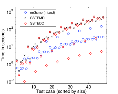
(a) Execution time: sequential.

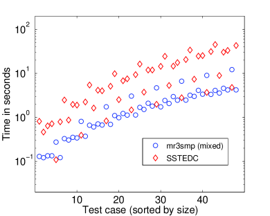
(b) Execution time: multi-threaded.

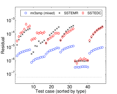
(c) Largest residual norm.

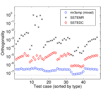
(d) Orthogonality.

Figure 1: Time and accuracy on Beckton. Timings are presented in a logarithmic scale. The largest residual norm and the orthogonality are measured as in (1). The dotted black line corresponds to unit round-off $\varepsilon_{s}$. As there exist no parallel MRRR for single precision, we show timings for our mixed precision approach and SSTEDC only.

As a reference, we include results for LAPACK’s SSTEMR (MRRR) and SSTEDC (Divide & Conquer). As shown in Fig. 1(a), even in a sequential execution, our mixed precision approach is up to an order of magnitude faster than LAPACK’s SSTEMR. For one type of matrices, SSTEDC is considerably faster than for all the others. These are the Wilkinson matrices, which represent a class of matrices that allow for heavy deflation within the Divide & Conquer approach. For all other matrices, which do not allow such extensive deflation, our solver is faster than SSTEDC. As seen in Fig. 1(b), in a parallel execution, the performance gap for the Wilkinson matrices almost entirely vanishes, while for the other matrices our solver remains up to an order of magnitude faster than SSTEDC. As depicted in Figs. 1(c)–1(d), our routine is not only as accurate as desired but it is the most accurate one. For single precision input/output arguments, we obtain a solver that is more accurate and faster than the original single precision solver. In addition, the solver is more scalable, and more robust. In 38 out of the 48 test cases, SSTEMR accepted representations that did not pass the test for relative robustness, thereby jeopardizing the accuracy of the result. In contrast, using mixed precisions, our solver was able to find suitable representations in all cases.

We now turn our attention to double precision inputs/outputs, for which timings and accuracy are presented in Fig. 2. We included the results for the multi-threaded solver mr3smp, which in the sequential case is just a wrapper to DSTEMR. In general, mr3smp obtains accuracy equivalent to LAPACK’s DSTEMR.

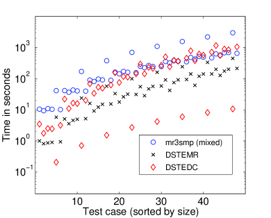
(a) Execution time: sequential.

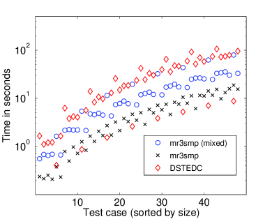
(b) Execution time: multi-threaded.

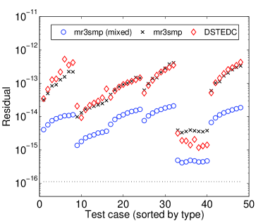
(c) Largest residual norm.

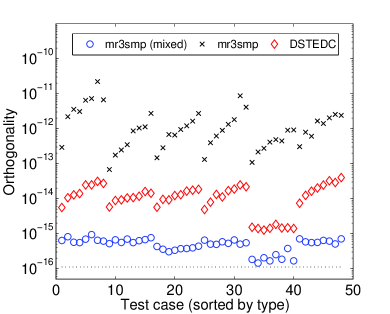
(d) Orthogonality.

Figure 2: Time and accuracy on Beckton. Timings are presented in a logarithmic scale. The largest residual and the orthogonality are measured as in (1). The dotted black line corresponds to unit round-off $\varepsilon_{d}$ and the accuracy of mr3smp is equivalent to the one obtained by LAPACK’s DSTEMR.

Figure 2(a) shows the timings for sequential executions. Our mixed precision solver is slower than DSTEMR, which is not a surprise, as we make use of software-simulated quadruple precision arithmetic. What might be a surprise is that, even with the use of such slow arithmetic, for large matrices, our solver is usually as fast as DSTEDC. As in the single precision case, only for matrices that allow for substantial deflation, DSTEDC is considerably faster. As Fig. 2(b) shows, for a parallel execution, the performance difference reduces and is expected to eventually vanish as it does already for the a regular MRRR implementation [32]. For matrices that do not allow for extensive deflation, our solver is about a factor two faster than DSTEDC.

While DSTEMR accepted in 29 out of the 48 test cases representations that did not pass the test for relative robustness, our mixed precision solver found suitable representations in all cases. In fact, for all but the Wilkinson type matrices, we have $d_{max}=0$ and as a consequence: no danger of failing to find suitable representations and embarrassingly parallel computation. Even for Wilkinson type matrices, $d_{max}$ was limited to one and clustering $\rho$ was limited to $2/n$. For DSTEMR, $d_{max}$ was as high as 21 and clustering $\rho$ was about $0.7$ on average, which should be compared with the value of about $1.6\cdot 10^{-4}$ for the mixed precision solver. Therefore, we believe that our approach is especially well-suited for highly parallel systems. In particular, solvers for distributed-memory systems should greatly benefit from better load-balancing and reduced communication.

For single precision inputs [Figs. 1(a)–1(b)] or in a parallel stetting [Fig. 2(b)], our tridiagonal eigensolver is highly competitive in terms of execution time – often faster – compared with Divide & Conquer and the conventional MRRR. As a consequence, when used in context of dense Hermitian eigenproblems, the accuracy improvement of the tridiagonal stage carry over to the overall accuracy without any penalty in terms of performance. Such a behavior is illustrated by Fig. 3, where we present timings and orthogonality for dense, real symmetric input matrices.

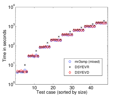
(a) Execution time: multi-threaded.

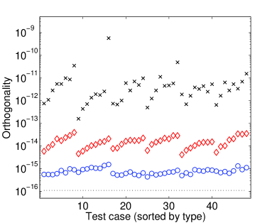
(b) Orthogonality.

Figure 3: Time and orthogonality for computing all eigenpairs of dense, real symmetric matrices. Timings are presented in a logarithmic scale and are dominated by the reduction to tridiagonal form.

The inputs were generated by applying random orthogonal similarity transformations to the tridiagonal matrices of the previous experiments: $A=QTQ^{*}$, with random orthogonal matrix $Q\in\mathbb{R}^{n\times n}$. For small matrices in a sequential execution, our approach introduces extra overhead – see Fig. 2(a). Since the tridiagonal solver only requires $\mathcal{O}(kn)$ operations to compute $k$ eigenpairs, while the reduction to tridiagonal form requires $\mathcal{O}(n^{3})$ operations, for sufficiently large matrices the overhead is completely negligible. Such a statement would even more apply if the matrices were complex-valued and/or only a subset of eigenpairs were computed, since the reduction to tridiagonal form would carry even more weight relative to the tridiagonal stage. In a parallel execution, the mixed precision approach is competitive even for relatively small matrices [Fig. 3(a)]; at the same time, the approach significantly improves orthogonality [Fig. 3(b)]. Further experiments, including subset computations and complex-valued inputs, can be found in [29, 33].

6 Conclusions

We presented a mixed precision variant of the MRRR algorithm, which addresses a number potential weaknesses of MRRR such as ($i$) inferior accuracy compared with the Divide & Conquer method or the QR algorithm; ($ii$) the danger of not finding suitable representations; and ($iii$) for distributed-memory architectures, load-balancing and communication problems for matrices with large clustering of the eigenvalues. Our approach provides a new perspective: Given input/output arguments in a binary_ x floating point format, we use a higher precision binary_y arithmetic to obtain the desired accuracy. As our analysis shows, the use of higher precision provides us with freedom in setting important parameters of the algorithm. In particular, we select these parameters to reduce the operation count, increase robustness, and improve parallelism; at the same time, we meet more stringent accuracy goals. Due to these changes, our mixed precision approach is not only as accurate as the Divide & Conquer method or the QR algorithm but – under many circumstances – is also faster than these methods or even faster than a conventional implementation of MRRR.

This work was mainly motivated by the results of MRRR-based eigensolvers for dense Hermitian problems [32]. In the context of dense eigenproblems, the tridiagonal stage is often completely negligible in terms of execution time: to compute $k$ eigenpairs of a tridiagonal matrix, it only requires $\mathcal{O}(kn)$ operations; the reduction to tridiagonal form requires $\mathcal{O}(n^{3})$ operations and is the performance bottleneck. In terms of accuracy, the tridiagonal stage is responsible for most of the loss of orthogonality. The natural question was whether it is possible to improve the accuracy to the level of the best methods without sacrificing too much performance. As our results show, this is indeed possible. In fact, our mixed precision solvers are even more accurate than the ones based on Divide & Conquer and QR, and remain as fast, or faster, than the classical MRRR. Finally, an important feature of the mixed precision approach is a considerably increased robustness and parallel scalability.

References

- [1] E. Anderson, Z. Bai, C. Bischof, S. Blackford, J. W. Demmel, J. Dongarra, J. D. Croz, A. Greenbaum, S. Hammarling, A. McKenney, and D. Sorensen. LAPACK Users’ Guide. SIAM, Philadelphia, PA, third edition, 1999.
- [2] P. Benner, P. Ezzatti, D. Kressner, E. S. Quintana-Ortí, and A. Remón. A Mixed-Precision Algorithm for the Solution of Lyapunov Equations on Hybrid CPU-GPU Platforms. Parallel Comput., 37(8):439–450, Aug. 2011.
- [3] P. Bientinesi, I. Dhillon, and R. van de Geijn. A Parallel Eigensolver for Dense Symmetric Matrices Based on Multiple Relatively Robust Representations. SIAM J. Sci. Comput., 27:43–66, 2005.
- [4] J. Cuppen. A Divide and Conquer Method for the Symmetric Tridiagonal Eigenproblem. Numer. Math., 36:177–195, 1981.
- [5] J. W. Demmel, J. Dongarra, A. Ruhe, and H. van der Vorst. Templates for the Solution of Algebraic Eigenvalue Problems: a Practical Guide. SIAM, Philadelphia, PA, USA, 2000.
- [6] J. W. Demmel, O. Marques, B. Parlett, and C. Vömel. Performance and Accuracy of LAPACK’s Symmetric Tridiagonal Eigensolvers. SIAM J. Sci. Comp., 30:1508–1526, 2008.
- [7] I. Dhillon. A New Algorithm for the Symmetric Tridiagonal Eigenvalue/Eigenvector Problem. PhD thesis, EECS Department, University of California, Berkeley, 1997.
- [8] I. Dhillon. Current Inverse Iteration Software Can Fail. BIT, 38:685–704, 1998.
- [9] I. Dhillon and B. Parlett. Multiple Representations to Compute Orthogonal Eigenvectors of Symmetric Tridiagonal Matrices. Linear Algebra Appl., 387:1–28, 2004.
- [10] I. Dhillon and B. Parlett. Orthogonal Eigenvectors and Relative Gaps. SIAM J. Matrix Anal. Appl., 25:858–899, 2004.
- [11] I. Dhillon, B. Parlett, and C. Vömel. Glued Matrices and the MRRR Algorithm. SIAM J. Sci. Comput, 27:496–510, 2005.
- [12] I. Dhillon, B. Parlett, and C. Vömel. The Design and Implementation of the MRRR Algorithm. ACM Trans. Math. Software, 32:533–560, 2006.
- [13] J. Dongarra, J. Du Cruz, I. Duff, and S. Hammarling. A Set of Level 3 Basic Linear Algebra Subprograms. ACM Trans. Math. Software, 16:1–17, 1990.
- [14] K. V. Fernando and B. Parlett. Accurate singular values and differential qd algorithms. Numerische Mathematik, 67:191–229, 1994.
- [15] J. Francis. The QR Transform - A Unitary Analogue to the LR Transformation, Part I and II. The Comp. J., 4, 1961/1962.
- [16] M. Gu and S. C. Eisenstat. A stable and efficient algorithm for the rank-one modification of the symmetric eigenproblem. SIAM J. Matrix Anal. Appl., 15(4):1266–1276, 1994.
- [17] M. Gu and S. C. Eisenstat. A Divide-and-Conquer Algorithm for the Symmetric Tridiagonal Eigenproblem. SIAM J. Matrix Anal. Appl., 16(1):172–191, 1995.
- [18] N. Higham. Iterative Refinement for Linear Systems and LAPACK. IMA Journal of Numerical Analysis, 17(4):495–509, 1997.
- [19] I. Ipsen. Computing An Eigenvector With Inverse Iteration. SIAM Review, 39:254–291, 1997.
- [20] V. Kublanovskaya. On some Algorithms for the Solution of the Complete Eigenvalue Problem. Zh. Vych. Mat., 1:555–572, 1961.
- [21] X. S. Li, J. W. Demmel, D. H. Bailey, G. Henry, Y. Hida, J. Iskandar, W. Kahan, A. Kapur, M. C. Martin, T. Tung, and D. J. Yoo. Design, Implementation and Testing of Extended and Mixed Precision BLAS. ACM Trans. Math. Software, 28:2002, 2002.
- [22] O. Marques, B. Parlett, and C. Vömel. Computations of Eigenpair Subsets with the MRRR Algorithm. Numerical Linear Algebra with Applications, 13(8):643–653, 2006.
- [23] O. A. Marques, C. Vömel, J. W. Demmel, and B. Parlett. Algorithm 880: A Testing Infrastructure for Symmetric Tridiagonal Eigensolvers. ACM Trans. Math. Softw., 35(1):8:1–8:13, 2008.
- [24] B. Parlett. The Symmetric Eigenvalue Problem. Prentice-Hall, Inc., Upper Saddle River, NJ, USA, 1998.
- [25] B. Parlett. Perturbation of Eigenpairs of Factored Symmetric Tridiagonal Matrices. Foundations of Computational Mathematics, 3:207–223, 2003.
- [26] B. Parlett and I. Dhillon. Fernando’s Solution to Wilkinson’s Problem: an Application of Double Factorization. Linear Algebra Appl., 267:247–279, 1996.
- [27] B. Parlett and I. Dhillon. Relatively Robust Representations of Symmetric Tridiagonals. Linear Algebra Appl., 309(1-3):121 – 151, 2000.
- [28] B. Parlett and O. Marques. An Implementation of the DQDS Algorithm (Positive Case). Linear Algebra Appl., 309:217–259, 1999.
- [29] M. Petschow. Eigensolvers for Multi-core Processors and Massively Parallel Supercomputers. PhD thesis, RWTH Aachen, Germany, in preparation.
- [30] M. Petschow and P. Bientinesi. The Algorithm of Multiple Relatively Robust Representations for Multi-Core Processors. volume 7133 of Lecture Notes in Computer Science, pages 152–161. Springer, 2010.
- [31] M. Petschow and P. Bientinesi. MR3-SMP: A Symmetric Tridiagonal Eigensolver for Multi-Core Architectures. Parallel Computing, 37(12):795 – 805, 2011.
- [32] M. Petschow, E. Peise, and P. Bientinesi. High-Performance Solvers For Dense Hermitian Eigenproblems. SIAM J. Sci. Comput., 35(1):1–22, 2013.
- [33] M. Petschow, E. Quintana-Ortí, and P. Bientinesi. Improved Orthogonality for Dense Hermitian Eigensolvers based on the MRRR algorithm. Technical Report AICES-2012/09-1, RWTH Aachen, Germany, 2012.
- [34] F. Tisseur and J. Dongarra. A parallel divide and conquer algorithm for the symmetric eigenvalue problem on distributed memory architectures. SIAM J. Sci. Comput., 20(6):2223–2236, 1999.
- [35] C. Vömel. A Refined Representation Tree for MRRR. LAPACK Working Note 194, Department of Computer Science, University of Tennessee, Knoxville, 2007.
- [36] C. Vömel. ScaLAPACK’s MRRR Algorithm. ACM Trans. Math. Software, 37:1:1–1:35, 2010.
- [37] P. Willems. On MR3-type Algorithms for the Tridiagonal Symmetric Eigenproblem and Bidiagonal SVD. PhD thesis, University of Wuppertal, Germany, 2010.
- [38] P. Willems and B. Lang. A Framework for the MR3 Algorithm: Theory and Implementation. Technical Report 11/21, Bergische Universität Wuppertal, Germany, 2011.
- [39] P. Willems and B. Lang. Block Factorizations and qd-type Transformations for the MR3 Algorithm. Electron. Trans. Numer. Anal., 38:363–400, 2011.
- [40] P. Willems and B. Lang. Twisted Factorizations and qd-Type Transformations for the MR3 Algorithm—New Representations and Analysis. SIAM Journal on Matrix Analysis and Applications, 33(2):523–553, 2012.