Emergence of slow collective oscillations
in neural networks with spike timing dependent plasticity

Abstract

The collective dynamics of excitatory pulse coupled neurons with spike timing dependent plasticity (STDP) is studied. The introduction of STDP induces persistent irregular oscillations between strongly and weakly synchronized states, reminiscent of brain activity during slow-wave sleep. We explain the oscillations by a mechanism, the “Sisyphus Effect”, caused by a continuous feedback between the synaptic adjustments and the coherence in the neural firing. Due to this effect, the synaptic weights have oscillating equilibrium values, and this prevents the system from relaxing into a stationary macroscopic state.

Sisyphus was the mythological king of Corinth compelled to roll a heavy boulder up a hill, only to watch it roll back down as it approached the top. Sisyphus was condemned by Zeus for his iniquity and pride to repeat eternally his efforts, without any hope of success. However, in the brain such endless motion can have a positive functional relevance. Fluctuating spontaneous activity has been observed in several areas of the brain harris . In particular, irregular oscillations between more and less synchronized states have been revealed in the hippocampus during slow-wave sleep and this activity has been related to memory consolidation in the neocortex buszaki1989 .

Recent studies have suggested synaptic plasticity as a fundamental ingredient to ensure multistability in neuronal circuits Tass2006BiolCyb ; Maistrenko2007Multistability ; Lubenov2008 ; mongillo2012 . In particular, spike timing dependent plasticity (STDP) is considered one of the central mechanisms underlying information elaboration and learning in the brain STDP . A series of experiments performed in vivo and in vitro on neural tissues revealed that the strength of a synapse, conveying spikes from a presynaptic to a postsynaptic neuron, depends crucially on the precise spike timing of the two connected neurons Markram1997Regulation ; Magee1997Synaptically ; Bi1998Synaptic . The STDP rules prescribe that whenever the presynaptic (postsynaptic) neuron fires before the postsynaptic (presynaptic) one, the synapse is potentiated (depressed). The synapse is modified only if the spikes occur within certain time intervals (learning windows). Asymmetric learning windows have repeatedly been found experimentally (e.g. see Bi2001Synaptic ; Bi2002Temporal ; FD ). This asymmetry is a prerequisite, at least in phase oscillator networks, to observe the coexistence of states characterized by different levels of synchrony Maistrenko2007Multistability ; Tass2006BiolCyb . Furthermore, in the presence of propagation delays STDP can provide a negative feedback mechanism contrasting highly synchronized network activity and promoting, in randomly driven networks, the emergence of states at the border between randomness and synchrony Lubenov2008 .

In this Letter a novel deterministic mechanism, the Sisyphus effect (SE), able to generate spontaneous fluctuations in a neural network between asynchronous and synchronous regimes is presented. In particular, we study excitatory pulse coupled neural networks with STDP, where the interaction among neurons is mediated by $\alpha$-pulses Abbott1993Asynchronous . For non plastic interactions, the excitatory coupling leads to synchronization only for sufficiently fast synapses Vreeswijk1994 . Furthermore, the desynchronizing effect is amplified at large coupling hansel1995 . In absence of plasticity the macroscopic activity of the network is stationary: asynchronous for large synaptic weights and partially synchronized for sufficiently weak coupling vanVreeswijk1996Partial ; hansel1995 .

The introduction of STDP completely modifies the dynamical landscape leading to a regime where a strongly and a weakly synchronized state coexist. The activity of the network is thus characterized by irregular oscillations between these two states. These transitions are driven by the evolution of the synaptic weights, which in turn is dictated by the level of synchrony in the network. For small synaptic weights the system is fully synchronized, while above a critical coupling it desynchronizes. Furthermore, whenever the network is synchronized (desynchronized) the synaptic weights tend towards large (small) equilibrium values corresponding to asynchronous (synchronous) dynamics. In summary, the neuronal activity can be represented in terms of an order parameter diffusing over an effective free energy landscape displaying two coexisting equilibrium states. Small (large) synaptic weights tilt the landscape towards the strongly (weakly) synchronized state, in turn the induced activity increases (reduces) the weights until a tilt in the opposite direction occurs. Thus the landscape oscillates endlessly.

The model. We study a fully coupled network of $N$ Leaky Integrate-and-Fire neurons, for which the membrane potential $V_{i}(t)\in[0:1]$ of neuron $i$ evolves as:

$$\dot{V}_{i}(t)=a-V_{i}(t)+I_{i}(t)\,\quad\quad i=1,\cdots,N\\ \quad,$$ (1)

whenever the neuron reaches the threshold $V_{i}=1$, an $\alpha$-pulse $p_{\alpha}(t)=\alpha^{2}t\exp(-\alpha t)$ is instantaneously transmitted to all other neurons and $V_{i}$ is reset to zero. Furthermore, $a>1$ is the suprathreshold DC current, $I_{i}=gE_{i}$ the synaptic current, and $g$ the excitatory homogeneous coupling. The field $E_{i}$ represents the linear superposition of the pulses received by neuron $i$ and its evolution is ruled by a second order ODE (Eq. (S2) in epabs ). For a fully coupled non-plastic network the synaptic weights associated to the connection from the presynaptic $j$-th neuron to the postsynaptic $i$-th one are $w_{ij}=1$ (apart from the autaptic terms: $w_{ii}=0$).

In the presence of plasticity, we assume that the weights evolve in time according to a nearest-neighbour STDP rule with soft bounds STDP ; Izhikevich2003BCM ; Maistrenko2007Multistability ; Chen2010Meanfield ; Chen2011 . Therefore in the case of a post- (presynaptic) spike, emitted by neuron $i$ ($j$) at time $t$, the weight $w_{ij}$ is potentiated (depressed) as $w_{ij}(t^{+})=w_{ij}(t^{-})+\Gamma_{ij}(t)$, with

$$\Gamma_{ij}(t)=\left\{\begin{array}[]{rcl}p[w_{M}-w_{ij}(t^{-})]{\rm e}^{-\frac{\delta_{ij}}{\tau_{+}}}&\mbox{if}&\delta_{ij}>0\\ &&\\ -d\,w_{ij}(t^{-}){\rm e}^{+\frac{\delta_{ij}}{\tau_{-}}}&\mbox{if}&\delta_{ij}<0\end{array}\right.$$ (2)

where $\delta_{ij}=t-t^{(j)}>0$ ($\delta_{ij}=t^{(i)}-t<0$) is the firing time difference and $t^{(k)}$ the last firing time of neuron $k$. The potentiation and depression factors ($p$ and $d$, resp.) coincide, unless otherwise specified quant . The bounds keep the synapses from achieving unrealistically large values or becoming inhibitory, namely $0\leq w_{ji}\leq w_{M}$. The learning windows over which post- (pre-) synaptic spikes will cause synaptic potentiation (depression) are indicated as $\tau_{+}$ ($\tau_{-}$). Following experimental evidences Bi2001Synaptic , we assume $\tau_{-}>\tau_{+}$. The degree of synchronization of the neurons is measured by the order parameter winfree ; kuram $R(t)=\left|\frac{1}{N}\sum_{k}e^{i\theta_{k}(t)}\right|$, where $\theta_{k}(t)=2\pi(t-t^{(k)}_{m})/(t^{(k)}_{m+1}-t^{(k)}_{m})$ is the phase of the $k$-th neuron at time $t$ between its $m$-th and $(m+1)$-th spike emission. A perfectly synchronized (asynchronous) system has $R=1$ ($R=0$), while intermediate values indicate partial synchronization.

Phase Diagram. We analyze how the phase diagram of the network is modified by the plasticity. In particular, we focus on the variation of the neuronal coherence by varying the DC current. Similar results can be obtained by varying the coupling $g$ and the pulse width $\alpha$ (as shown in epabs ). To compare with previous results obtained without plasticity, we fix $g=0.4$ and $\alpha=9$ as in vanVreeswijk1996Partial ; zillmer2007 . In absence of plasticity the homogeneous system exhibits two phases: an asynchronous regime with $R\equiv 0$, and a partially synchronized phase with finite $R$ vanVreeswijk1996Partial . The emergence of one or the other regime depends crucially on the ratio of two time scales: the pulse rise time $1/\alpha$ and the interspike-interval (ISI) Vreeswijk1994 ; zillmer2007 . For slow synapses (relative to the ISI) the system dynamics is asynchronous, while for sufficiently fast synapses coherent oscillations emerge. The system becomes fully synchronized only for instantaneous synaptic rise times (i.e. $\alpha\to\infty$). For fixed network size $N$ and pulse shape, the ISI can be reduced by increasing either the external DC current or the synaptic coupling. Therefore partial synchronization is observable for sufficiently small $a$ or $g$ values (whenever $\alpha\gtrsim 3.4$), while incrementing these parameters will desynchronize the system hansel1995 (as shown in Fig. 1a in epabs ).

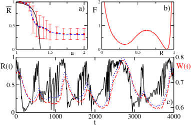
Figure 1: (color online) (a) Average order parameter $\bar{R}$ as a function of $a$ for the non plastic network (black solid line) and in the presence of STDP for $N=200$ (red filled squares) and $N=500$ (blue dashed line) (b) Free energy profile $F(R)$ versus $R$ for $N=200$, obtained by evaluating $R$ at regular time intervals $\Delta t=1$ for a time span $\sim 5\times 10^{6}$. (c) Time evolution of $R(t)$ (black solid line) and of $W(t)$ (red dashed line) for $N=500$. The dotted (blue) line is the $W$ predicted via Eq. (3). The data refer to $a=1.3$, $g=0.4$, $\alpha=9$, $d=p=0.01$, $\tau_{-}=3\tau_{+}=0.3$, and $w_{M}=2$, and are measured after a transient $\sim 10^{5}$.

The average level of synchronization $\bar{R}$ is reported in Fig. 1a as a function of $a$ for the non-plastic and plastic cases. In absence of plasticity the system is partially synchronized for low DC currents and asynchronous for $a\geq a_{c}\simeq 1.35$. The introduction of plasticity does not alter the scenario at small $a$-values, where the system is in a high synchronization (HS) regime. The main difference is observable in the dynamics of $R(t)$, which displays irregular oscillations: the associated Fourier spectrum resembles a Lorentzian with a small subsidiary peak around period $\simeq 34-36$. However, for sufficiently large currents, namely $a>1.5$, the asynchronous regime is substituted by a state of low synchronization (LS) characterized by a rapidly fluctuating order parameter (over a time scale of the order of 70 - 150) with an associated small level of synchronization $\bar{R}\simeq 0.32\pm 0.12$. At intermediate $a$-values, in the range $a\in[1.23;1.46]$, $R$ exhibits wide irregular temporal oscillations between values $\simeq 1$ and zero with characteristic time scales $\simeq 1100-1400$. These latter oscillations represent low frequency fluctuations (LFFs), while rapid fluctuations are still present over time scales $\simeq 50-60$ (see Fig. 1c).

In this Letter we will mainly focus on the intermediate regime, fixing $a=1.30$, where the LFF of $R(t)$ resembles the evolution of a particle in a double well potential subject to thermal fluctuations. To clarify this analogy we have estimated the PDF, $P(R)$, of the order parameter, by examining its trajectory for a sufficiently long time span, and derived the associated free energy profile as $F(R)=-\log P(R)$. As shown in Fig. 1b, $F(R)$ exhibits two minima corresponding to a HS phase at $R_{H}\simeq 0.905$ and a LS state at $R_{L}\simeq 0.32$. The 2 coexisting minima are separated by a saddle, located at $R_{S}\simeq 0.61$. As clarified in the following the jumps between minima are driven by the macroscopic evolution of network plasticity. The rapid fluctuations, present in all regimes, are instead due to the microsopic evolution of the synaptic weights, which can be interpreted as a noise source for the dynamics of $R(t)$. The analysis of these noise-induced oscillations goes beyond the scope of this Letter and it is left for future studies.

Constrained phase diagram As shown in Fig. 1c the LFFs of $R(t)$ are associated with oscillations in the average synaptic weight $W(t)\equiv\sum_{i,j}w_{ji}(t)/N(N-1)$. In particular when the system is in a HS (LS) state $W$ increases (decreases).

To better investigate the origin of these correlations and the interaction between the STDP induced synaptic dynamics and the level of synchronization in the system we perform the following numerical experiments. We simulate the system by constraining the synaptic weights to have a constant average value $W_{0}$, by rescaling, at regular time intervals, the weights $w_{ij}$. Initially, $W_{0}=0$ and we follow the evolution of the system for a time span $T_{S}$. We then perform a new simulation for the same time lapse with a larger $W_{0}$ value, starting from the last configuration of the previous run. The procedure is repeated by increasing $W_{0}$ at regular steps $\Delta W_{0}$ until $W_{0}=w_{M}$ is reached. Then with the same protocol $W_{0}$ is decreased (in steps of $\Delta W_{0}$) until finally $W_{0}$ returns to zero note3 . The results of these simulations are shown in Fig. 2 for $N=200$. At low $W_{0}$ the system is fully synchronized, while with increasing $W_{0}$ the system desynchronizes via a discontinuous transition. By further increasing $W_{0}$ the level of synchronization continues to decrease and another smooth transition seems to occur. For the explanation of the SE it is sufficient to limit the analysis to the first transition.

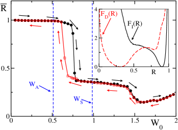
Figure 2: (color online) $\bar{R}$ versus $W_{0}$ as measured for increasing (black filled circles) and decreasing (empty red squares) $W_{0}$. The (blue) vertical dashed lines indicate the fixed point values $W_{S}$ and $W_{A}$ epabs . Results averaged over 8 different initial conditions, $T_{S}=1,000$, $\Delta W_{0}=0.02$ (for clarity only one point every two is shown). (Inset) Conditional free energy profiles $F_{I}(R)$ (black solid line) and $F_{D}(R)$ (red dashed line) obtained during USs. Both curves are vertically shifted to achieve zero as minimal value. Parameters as in Fig. 1 and $N=200$.

As shown in Fig. 2, the constrained system exhibits a hysteretic transition from HS to LS (from LS to HS) for $W_{0}^{(1)}=0.76(5)$ ($W_{0}^{(2)}=0.65(5)$) by increasing (decreasing) the control parameter $W_{0}$ note2 . This implies that in the interval $[W_{0}^{(2)},W_{0}^{(1)}]$ the two regimes coexist and that HS or LS is observable depending on the initial state of the network.

Mean field synaptic evolution. In order to gain some insight into the evolution of the system during unconstrained simulations (USs), let us consider a mean field equation for the synaptic weight evolution. The average synaptic weight modification $\Gamma$, for each presynaptic spike, can be written as Izhikevich2003BCM

$$\Gamma(t)=p(w_{M}-W)\int_{0}^{\infty}d\delta P(\delta){\rm e}^{\frac{-\delta}{\tau_{+}}}-dW\int_{-\infty}^{0}d\delta P(-\delta){\rm e}^{\frac{\delta}{\tau_{-}}}$$ (3)

where $P(\delta)$ is the PDF of the time differences $\delta$ between postsynaptic and presynaptic firing measured. To test the predictive value of Eq. (3), we have measured from an US $P(\delta)$ at regular intervals $\Delta t$. By employing this information we can predict quite well the evolution of the synaptic weight as $W(t+\Delta t)=W(t)+\Gamma(t)$ (see Fig. 1c).

By assuming that the postsynaptic neuron is firing with period $T_{0}$, we are able to derive the time difference distribution $P(\delta)$ for the two limiting cases: fully synchronized and asynchronous dynamics. In the fully synchronized (asynchronous) situations we expect a distribution of the form $P_{S}(\delta)={\cal D}(\delta)+{\cal D}(\delta-T_{0})$ ($P_{A}(\delta)=1/T_{0}$) defined in the interval $[0:T_{0}]$. Here ${\cal D}$ denotes a Dirac delta function. These guesses are essentially confirmed by direct USs as shown in Fig. 3 in epabs . Therefore in these two cases an analytical estimation of $\Gamma$ can be obtained. Furthermore, in both cases $\Gamma$ vanishes for a finite value of the average synaptic weight, namely $W_{S}$ ($W_{A}$) for the synchronized (asynchronous) situation. Furthermore, for $W<W_{S}$ ($W>W_{S}$) the synapses are in average potentiated (depressed) and analogously for the asynchronous case. This implies that $W_{S}$ ($W_{A}$) is a stable attractive point for the dynamics of $W$ in the synchronized (asynchronous) regime (for a definition of $W_{S}$ and $W_{A}$ see Eq. (S8) and (S10) in epabs ).

Sisyphus mechanism. We are now able to explain the behavior reported in Fig. 1c for $R(t)$ and $W(t)$. Let us suppose that the system is in the HS phase with an associated low coupling $W<W_{0}^{(1)}$. However, in this situation the attractive fixed point $W_{S}$ is above the transition point $W_{0}^{(1)}$ (see Fig. 2). Therefore $W$ keeps increasing, until for $W>W_{0}^{(1)}$ the system starts to desynchronize and to approach the LS state. In this phase the $P(\delta)$ becomes almost flat (see Fig. 3b in epabs ) and the attractive point for the synaptic evolution will be $W_{A}$, located below $W_{0}^{(2)}$. The motion towards $W_{A}$ leads to a decrease of $W$. Whenever the average synaptic weight crosses $W_{0}^{(2)}$ the neurons begins to resynchronize. Finally, the system will return to the HS state from where it started. The cycle will repeat indefinitely and is the essence of the SE.

The above arguments are approximate, because the system is never exactly fully synchronized or desynchronized, instead it passes through a continuum of states, each associated to a different fixed point in $W$-space. The relevant aspect is that the fixed points associated to the HS (LS) phase are larger than the transition point $W_{0}^{(1)}$ (smaller than $W_{0}^{(2)}$). As we have verified this is indeed the case, therefore the mechanism is still valid. To perform a direct test of the validity of our analysis, we have measured the PDF of $R$ conditioned to the fact that $W$ was increasing (decreasing) during an US. From these PDFs we derived the corresponding free energy profile $F_{I}(R)$ ($F_{D}(R)$). As shown in the inset of Fig. 2 $F_{I}$ has a unique minimum at $R_{H}$, while $F_{D}$ has an absolute minimum at $R_{L}$ and a shoulder around $R\simeq 0.8$. These results confirm that the equilibrium attractive values for $W$ are located opposite to the transition points, because when the system is in the HS (LS) regime the synaptic weights increase (decrease) continuously trying to reach the corresponding fixed points.

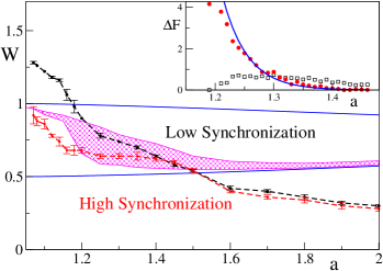
Figure 3: (color online) $W$ versus the DC current $a$. The shaded area represents the $W$-values measured during USs. The upper black (lower red) dashed line refers to the estimated $W_{0}^{(1)}$ ($W_{0}^{(2)}$). The error bars have been evaluated over 5 different realizations of the constrained simulations. The upper (lower) solid blue line represents the fixed point values $W_{S}$ ($W_{A}$). (Inset) The red circles (black squares) refer to the free energy barrier $\Delta F$ separating the HS (LS) state from the saddle. The blue line is an exponential fit to the HS barrier height. The remaining parameters as in Fig. 1 and $N=500$

The SE should be active whenever the transition values $W_{0}^{(1)}$ and $W_{0}^{(2)}$ are both contained within the interval $[W_{A},W_{S}]$. To verify this statement we have measured $W_{0}^{(1)}$, $W_{0}^{(2)}$ and the fixed points for various DC currents within the interval $0<a\leq 2$ (data shown in Fig. 3). We observe that the transition is hysteretic in the interval $a\in]0;1.40]$, while for larger values $W_{0}^{(1)}$ and $W_{0}^{(2)}$ essentially coincide. Furthermore, $W_{0}^{(1)}$ becomes larger than $W_{S}$ at $a\simeq 1.18$, while $W_{A}\geq W_{0}^{(1)},W_{0}^{(2)}$ for $a\geq 1.50$. Thus we expect that $F(R)$ exhibits two coexisting minima, due to the SE, when $1.18\leq a\leq 1.50$. To verify this conjecture we estimate the free energy barrier heights $\Delta F$ separating the HS and the LS state from the intermediate saddle for various $a$ values. As shown in the inset of Fig. 3, the barrier associated to the HS state diverges exponentially when approaching $a\simeq 1.18$. Therefore, the HS regime is the only possible at smaller $a$-values. On the other hand the two minima merge and the associated barriers vanish for $a\geq 1.48$ indicating that the LS state is the unique remaining at large $a$. Furthermore, the distributions of the $W$-values measured during USs are reported in Fig. 3 as a shaded area: these values include the transition interval $[W_{0}^{(1)};W_{0}^{(2)}]$ for $1.20\leq a\leq 1.48$.

In conclusion, the SE should be observable in pulse coupled neural networks whenever the excitation has a desynchronizing effect. This is in general verified for any kind of neuronal response (type I or type II) for sufficiently slow synaptic interactions Vreeswijk1994 ; hansel1995 . Furthermore, we have verified that the SE persists by setting $p>d$, as suggested by experimental evidences FD .

ADDITIONAL MATERIAL

I The Model

We study a fully coupled network of $N$ Leaky Integrate-and-Fire (LIF) neurons, for which the membrane potential $V_{i}(t)\in[0:1]$ of neuron $i$ evolves as:

$$\dot{V}_{i}(t)=a-V_{i}(t)+I_{i}(t)\,\quad\quad i=1,\cdots,N\\ \quad,$$ (4)

where $a>1$ is the suprathreshold DC current, and $I_{i}$ the synaptic current due to the coupling with the rest of the network. Following abbott_vanvreeswik , we assume that whenever the $i$-th neuron reaches the threshold $V_{i}=1$, an $\alpha$-pulse $p_{\alpha}(t)=\alpha^{2}t\exp(-\alpha t)$ is instantaneously transmitted to all the other neurons and its membrane potential is reset to $V_{i}=0$. The synaptic current can be written as $I_{i}(t)=gE_{i}(t)$, with $g>0$ representing the excitatory homogeneous coupling while the field $E_{i}(t)$ is given by the linear superposition of the pulses received by neuron $i$ in the past. For $\alpha$-pulses the time evolution of the field $E_{i}(t)$ is ruled by the following second order differential equation:

$$\ddot{E}_{i}(t)+2\alpha\dot{E}_{i}(t)+\alpha^{2}E_{i}(t)=\frac{\alpha^{2}}{N-1}\sum_{n|t_{n}<t}w_{ij}\delta(t-t_{n})\ .$$ (5)

with $\{t_{n}\}$ being the firing times until the present time $t$. For a fully coupled network, in absence of plasticity, the synaptic weights $w_{ij}$ appearing in Eq. (5) are all equal to one (apart from the autaptic terms which are set to zero). In presence of plasticity, we assume that the synaptic weights evolve in time according to a STDP rule with soft bounds, namely STDP ; Maistrenko2007Multistability ; Chen2010Meanfield

$$\dot{w}_{ij}(t)=p(w_{max}-w_{ij}(t))A_{j}S_{i}-dw_{ij}(t)B_{i}S_{j}\quad,$$ (6)

where $d$ (resp. $p$) is the potentiation (resp. depression) amplitude, and $S_{k}$ represents the series of spiking times of neuron $k$ until time $t$. The presence of the bounds implies that $0\leq w_{ij}\leq w_{max}$. By assuming that the synapses have memory just of the last emitted spike (nearest-neighbour STDP rule), the variables $A_{j}$ (resp. $B_{i}$) evolves as follows STDP ; Chen2010Meanfield

$$\tau_{+}\dot{A_{j}}=-A_{j}+(1-A_{j})S_{j}\enskip,\enskip\tau_{-}\dot{B_{i}}=-B_{i}+(1-B_{i})S_{i}$$ (7)

where $\tau_{+}$ (resp. $\tau_{-}$) are the time windows over which post- (resp. pre-) synaptic spikes will cause potentiation (resp. depression) of the synapse. As pointed out by Izhikevich and Desai Izhikevich2003BCM the nearest neighbour implementation of the STDP rule is the only one consistent with the classical results on long-term potentiation and depression by Bienenstock-Cooper-Munro BCM

Therefore in the case of a post-synaptic (pre-synaptic) spike, emitted by neuron $i$ ($j$) at time $t$, the weight $w_{ij}$ is potentiated (depressed) as $w_{ij}(t^{+})=w_{ij}(t^{-})+\Gamma_{ij}(t)$, with

$$\Gamma_{ij}(t)=\left\{\begin{array}[]{rcl}p[w_{M}-w_{ij}(t^{-})]{\rm e}^{-\frac{\delta_{ij}}{\tau_{+}}}&\mbox{if}&\delta_{ij}>0\\ &&\\ -d\,w_{ij}(t^{-}){\rm e}^{+\frac{\delta_{ij}}{\tau_{-}}}&\mbox{if}&\delta_{ij}<0\end{array}\right.$$ (8)

where $\delta_{ij}=t-t^{(j)}>0$ ($\delta_{ij}=t^{(i)}-t<0$) is the firing time difference and $t^{(k)}$ the last firing time of neuron $k$.

Since the plasticity rule depends critically on the precision of the spiking events, it is necessary to employ an accurate integration scheme to update the evolution equations. For this purpose we adopted an event-driven algorithm with event queue conjugating high accuracy with a fast implementation zillmer2007 ; Chen2011 .

The degree of synchronization of the neuronal population can be characterized in terms of the order parameter winfree ; kuram

$$R(t)=\left|\frac{1}{N}\sum_{k}e^{i\theta_{k}(t)}\right|\quad,$$ (9)

where

$$\theta_{k}(t)=2\pi\frac{(t-t^{(k)}_{m})}{(t^{(k)}_{m+1}-t^{(k)}_{m})}$$ (10)

is the phase of the $k$-th neuron at time $t$ between its $m$-th and $m+1$-th spike emission, occurring at times $t^{(k)}_{m}$ and $t^{(k)}_{m+1}$, respectively. A non zero $R$ value is an indication of partial synchronization, perfect synchronization is achieved for $R=1$, while a vanishingly small $R\sim 1/\sqrt{N}$ is observable for asynchronous states in finite systems.

II Phase Diagram

We report in Fig. 4 the phase diagram for the non plastic fully connected network for $N=100$ in the planes $(g,a)$ and $(g,\alpha)$. In this case the asynchronous regime corresponds to a so-called splay state abbott_vanvreeswik ; zillmer2007 : this is an exact solution for the system which is perfectly asynchronous ($R\equiv 0$). For this periodic solution we are able to perform an analytical stability analysis zillmer2007 , reported in Fig. 4. The (green) circles in Fig. 4 indicates the marginal stability line for the the splay state, it is known that whenever the splays state looses its stability it gives rise to a partially synchronized regime via a Hopf supercritical bifurcation  abbott_vanvreeswik . With reference to the parameter values considered in this Letter, partial synchronization emerges for $a\leq a_{c}\simeq 1.35$ for fixed coupling $g=0.4$, and for $g\leq g_{c}\simeq 0.4676$ for fixed pulse width $\alpha=9$.

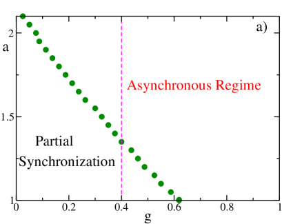
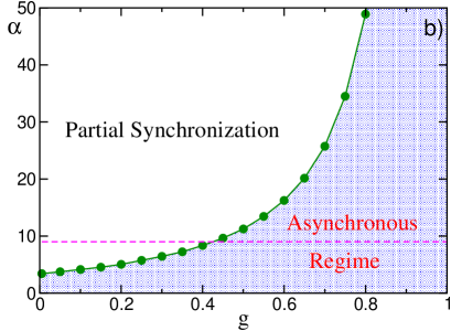
Figure 4: (color online) Phase diagram for the homogeneous model without plasticity in (a) we report the phase plane $(g,a)$, while in (b) the phases are shown in the $(g,\alpha)$-plane. The (green) filled circles indicate the critical values for which the asynchronous state (namely, the splay state) becomes unstable; the dashed (magenta) line refers to $g=0.4$ in (a) and $\alpha=9$ in (b). The other parameters are fixed to $\alpha=9$ in (a) and $g=0.4$ in (b) and the system size is $N=100$.

In order to characterize the dynamical phases observed in the plastic and non plastic networks, we have also estimated the order parameter $\bar{R}$ averaged over a certain time span.

The behaviour of $\bar{R}$ as a function of $g$ and $\alpha$ are reported in in Fig. 5, similarly to the non plastic case the system desynchronizes also in presence of STDP for increasing synaptic coupling $g$ and pulse rise times $1/\alpha$. However, the perfectly asynchronous regime is substituted by a low synchronization phase where $\bar{R}\sim 0.2$. Furthermore in proximity of the transition region from high synchronous to the low synchronous regime $R(t)$ exhibits large low frequency fluctuations as in the case studied in the Letter.

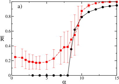
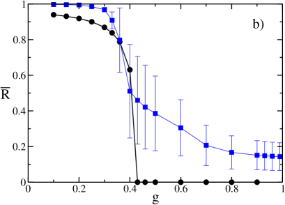
Figure 5: (color online) (a) Average order parameter $\bar{R}$ versus $\alpha$ for the systems without plasticity (black circles) and with STDP (red squares); (b) $\bar{R}$ versus $g$ for the systems without plasticity (black circles) and with STDP (blue squares). The parameters are $a=1.3$ and $N=200$, in (a) $g=0.4$ and in (b) $\alpha=9$. The average have been performed over time spans $\simeq 10^{4}-10^{5}$ time units, after discarding transients of duration $\simeq 10^{4}-10^{5}$.

III Time difference distributions

The probability density distributions (PDF) for the time differences $\delta$ between postsynaptic and presynaptic firing time can be easily derived in two limiting case by assuming a constant inter-spike interval (ISI) $T_{0}$ for the post-synaptic neuron. For fully synchronized neurons, we expect the pre- and postsynaptic neurons to fire together $\delta=0$ or with a delay given by the ISI, namely $\delta=T_{0}$. Therefore the distribution will be $P_{S}(\delta)={\cal D}(\delta)+{\cal D}(\delta-T_{0})$, where ${\cal D}(x-x_{0})$ denotes a Dirac delta function centered in $x_{0}$. The other situation we consider is that corresponding to perfect asynchrony, in this case we expect that $\delta$ will take all values in the interval $[0:T_{0}]$ and all the values will be equiprobable therefore we expect $P_{A}(\delta)=1/T_{0}$.

In Fig. 6 we compare the predictions with the measured distributions, the agreement is reasonable in view of the fact that the two considered states do not correspond exactly to $R=1$ and $R=0$ and that the ISI is not constant over all the neuronal population. Therefore, we can consider $P_{A}(\delta)$ and $P_{S}(\delta)$ as reasonable approximation of the true distributions in the two extreme cases achieved by the system during its evolution.

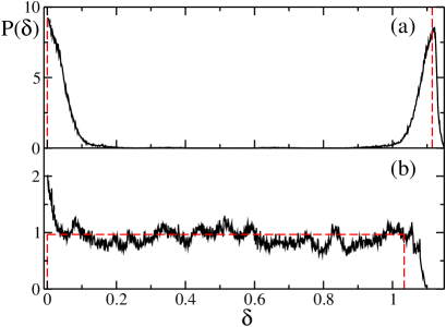
Figure 6: (color online) Probability distribution functions $P(\delta)$ as obtained during an unconstrained simulation by considering the $N\times(N-1)$ $\delta_{ij}$ values associated to the last $N$ spikes preceeding a strongly (resp. weakly) synchronized state corresponding to an order parameter value $R\simeq 0.98$ (resp. $R\simeq 0.11$). The estimated PDF are reported in panel (a) and (b), respectively. The red dashed lines refer to $P_{S}$ in (a) and $P_{A}$ in (b) defined in the text. The parameters of the simulation are $\alpha=9$, $\tau_{-}=3\tau_{+}=0.30$, $d=p=0.01$, $g=0.4$ and the network size is $N=500$

IV Mean field synaptic evolution

By assuming that the post-synaptic neuron fires with constant period $T_{0}$ we can perform the integrals appearing in Eq. (3) in the letter in the 2 limiting cases discussed above.

IV.1 Asynchronous dynamics

In this situation $P(\delta)=P_{A}(\delta)$ and we can rewrite Eq. (3) as follows

$$\Gamma_{A}=\frac{p\tau_{+}}{T_{0}}\left[(w_{M}-W)(1-{\rm e}^{-\frac{T_{0}}{\tau_{+}}})-3W(1-{\rm e}^{-\frac{T_{0}}{\tau_{-}}})\right]$$ (11)

where we have assumed $p=d$ and $\tau_{-}=3\tau_{+}$ as for the most part of the simulations studied in the Letter. The quantity $\Gamma_{A}$ vanishes for $W=W_{A}$ and it is positive (resp. negative) for $W<W_{A}$ (resp. $W>W_{A}$), therefore for the dynamics of $W(t)$

$$W_{A}=\frac{w_{M}\left(1-{\rm e}^{-\frac{T_{0}}{\tau_{+}}}\right)}{4-{\rm e}^{-\frac{T_{0}}{\tau_{+}}}-3{\rm e}^{-\frac{T_{0}}{\tau_{-}}}}$$ (12)

is a stable fixed point.

IV.2 Fully synchronized dynamics

For the fully synchronized situation $P(\delta)=P_{S}(\delta)$ and Eq. (3) becomes

$$\Gamma_{S}=p\left[w_{M}(1+{\rm e}^{-\frac{T_{0}}{\tau_{+}}})-W(2+{\rm e}^{-\frac{T_{0}}{\tau_{+}}}+{\rm e}^{-\frac{T_{0}}{\tau_{-}}})\right]$$ (13)

where we have assumed once more $p=d$ and $\tau_{-}=3\tau_{+}$. The quantity $\Gamma_{S}$ vanishes for $W=W_{S}$ and it is positive (resp. negative) for $W<W_{S}$ (resp. $W>W_{S}$), therefore the solution

$$W_{S}=\frac{w_{M}\left(1+{\rm e}^{-\frac{T_{0}}{\tau_{+}}}\right)}{2+{\rm e}^{-\frac{T_{0}}{\tau_{+}}}+{\rm e}^{-\frac{T_{0}}{\tau_{-}}}}$$ (14)

represents an attractive fixed point.

References

- (1) L. F. Abbott and C. van Vreeswijk, Phys. Rev. E 48, 1483 (1993).
- (2) J. Sjöström and W. Gerstner, Scholarpedia 5(2), 1362 (2010).
- (3) Y. L. Maistrenko,B. Lysyansky,C. Hauptmann,O. Burylko, and P.A. Tass, Physical Review E 75, 066207 (2007).
- (4) C. C. Chen and D. Jasnow, Physical Review E 81, 011907 (2010).
- (5) E. M. Izhikevich and N. S. Desai, Neural Comput. 15, 1511 (2003).
- (6) E. Bienenstock, L. Cooper, and P. Munro, The Journal of Neuroscience 2, 32 (1982).
- (7) R. Zillmer, R. Livi, A. Politi, and A. Torcini, Phys. Rev. E 76, 046102 (2007).
- (8) C. C. Chen and D. Jasnow, Phys. Rev. E 84, 031908 (2011).
- (9) A. Winfree, The Geometry of Biological Time (Springer-Verlag, Berlin-Heidelberg-New York, 1980).
- (10) Y. Kuramoto, Chemical Oscillations, Waves, and Turbulence, Dover Books on Chemistry Series (Dover Publications, New York, 2003).