Uniqueness and Significance of Weak Solution of Non-perturbative Renormalization Group Equation
to Analyze Dynamical Chiral Symmetry Breaking

Abstract

We propose quite a new method of analyzing the dynamical chiral symmetry breaking in gauge theories. Starting with the non-perturbative renormalization group equation for the Wilsonian fermion potential, we define the weak solution of it in order to mathematically authorize solutions with singularity. The weak solution is obtained uniquely and it successfully predicts the physically correct vacuum, chiral condensates, dynamical mass, through its auto-convexizing power for the effective potential. Thus it works perfectly even for the first order phase transition in the finite density QCD.

I Introduction

Among various methods to analyze the dynamical chiral symmetry breaking, the non-perturbative renormalization group is quite effective since it may include non-ladder diagrams which cure the gauge invariance problemSato13 . In the lowest order approximation, the Wilsonian effective action is expressed by a scale dependent fermion potential $V_{\rm W}(x,t)$, where $x=\int d^{4}x\bar{\psi}(x)\psi(x)$ is an operator variable, $t=\log(\Lambda_{0}/\Lambda(t))$ is the renormalization scale. This potential keeps all information of the fermionic interactions, the free energy $V_{0}$, the dynamical mass $M_{d}$, the 4-fermion interactions G etc as follows:

$$V_{\rm W}(x,t)=V_{0}(t)+M_{d}(t)x+G(t)\frac{x^{2}}{2}+\cdots.$$ (1)

The renormalization group equation for $G$ (in case $M=0$) is written as

$$\frac{dG}{dt}=-2G+\frac{1}{2\pi^{2}}G^{2},$$ (2)

which makes $G$ diverge at a finite scale $t_{\rm c}$ for upper critical initial value. This blowup nature itself is a correct behavior since it expresses the divergence of the susceptibility due to the spontaneous chiral symmetry breakdownAoki96 ; Aoki99 . However, due to this divergence we can not go beyond $t_{\rm c}$, and there is no way to calculate infrared physical quantities such as the chiral condensate or the dynamical mass.

II Partial differential equation and its weak solution

Various methods have been used to bypass this singularity, e.g., the bare massMiya09 , auxiliary fieldsAoki96 ; Aoki99 ; Gies02 , etc. Here we propose a new direct method of solving the renormalization group equation as a partial differential equation (PDE)Kuma13 :

$$\frac{\partial M(x,t)}{\partial t}+\frac{\partial f(M(x,t),t)}{\partial x}=0,\ M=\frac{\partial V_{\rm W}}{\partial x},\ f(M,t)=-\frac{1}{4\pi^{2}}e^{-4t}\ln[1+M^{2}e^{2t}],$$ (3)

where $M(x,t)$ is called the mass function. The 4-fermion interaction $G$ corresponds to $\frac{\partial M}{\partial x}$ at the origin, and its divergence at finite $t_{\rm c}$ means that the above PDE has no global classical solution beyond $t_{\rm c}$.

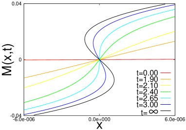
(a) (b)

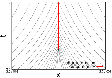
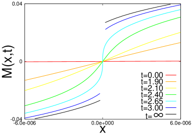
(c) (d)

Figure 1: NJL plot. (a) Characteristics. (b) Mass function. (c) Discontinuity. (d) Weak solution.

The expected behavior of physically meaningful solution $M(x,t)$ is plotted in Fig. 1(d), where $M$ has a jump at the origin after $t_{\rm c}$. In order to accommodate such singular solution with discontinuity, we write down the weak version of the PDEKuma13 ; Eva01 ,

$$\int_{0}^{\infty}dt\int_{-\infty}^{\infty}dx\left[M\frac{\partial\varphi}{\partial t}+f(M,t)\frac{\partial\varphi}{\partial x}\right]+\int_{-\infty}^{\infty}dx~{}M(x,0)\varphi(x,0)=0.$$ (4)

The weak solution is defined as to satisfy the above equation for any smooth and bounded test function $\varphi(x,t)$. The weak solution satisfy original PDE except for discontinuity and position of discontinuity $x=S(t)$ is controlled by the Rankine-Hugoniot (RH) condition,

$$\frac{dS(t)}{dt}[M_{+}-M_{-}]=f(M_{+})-f(M_{-}),$$ (5)

where $M_{+},M_{-}$ are right and left limit at the discontinuity point respectively.

To obtain the weak solution, first we set up characteristic curves $x=X(t)$ representing the contour lines of $M$, which satisfies

$$\frac{dX(t)}{dt}=\frac{\partial f(M,t)}{\partial M}.$$ (6)

Where these curves are crossing each other, we must pick up one curve and introduce discontinuity according to the RH condition, and then we get the unique function $M(x,t)$. Fig. 1 shows the Nambu-Jona-Lassinio (NJL) model example ($g=1.005g_{\rm c}$) of these procedures. The contour lines are plotted in (a), where at some finite $t_{\rm c}$ they start crossing with each other. The cross section of the total contours is seen in (b), where the derivative $\frac{\partial M}{\partial x}$ diverges at the origin at some $t_{\rm c}$.

Note that in obtaining $M(x,t)$ as in (b) there is nothing singular, and it is just a motion of ‘string’. However, to get the renormalized potential we have to define $M(x,t)$ as a unique function of $x$. Then the RH condition determines the discontinuity as shown in (c), and the mass function in (d). This is the weak solution of the PDE and it defines global $t$ solution uniquely.

III Weak solution results for the physical quantities

We show results in the finite density NJL where the first order phase transition occurs. Contours and mass function are plotted in Fig. 2, where at the central region five-fold structure appears corresponding to the three-fold local minima. In the renormalization procedure, two discontinuities appear pairwisely, move towards the origin, and finally merge into one at the origin as shown in Fig. 2(a).

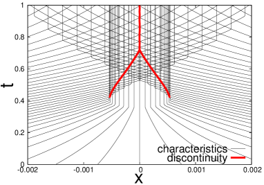
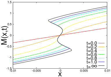
(a) (b)

Figure 2: NJL $g=1.7g_{\rm c},~{}\mu=0.7$. (a) Characteristics and jumps. (b) Evolution of mass function.

Snapshots in the course of renormalization are shown in Fig. 3, where the mass function $M(t,x)$, the Wilsonian fermion potential $V_{\rm W}$ and the Legendre effective potential for $\sigma$ are plotted. It is astonishing that our method of weak solution uniquely determines their singularity structures and the resultant Legendre effective potential is always convexized. This means the dynamical mass and the chiral condensates are uniquely calculated, and perfectly correct in the sense that even in case there are multi local minima, the lowest free energy minimum is always chosen automatically. This feature is quite a new finding and shows powerfulness of the purely fermionic non-perturbative renormalization group and its weak solutionKuma13 . This analysis has been applied to QCD, even with finite density or non-ladder, and proved to work perfectly to give physical quantities without any ambiguitySato13 .

(1a) (1b) (1c)

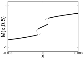
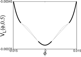
(2a) (2b) (2c)

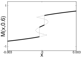
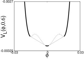
(3a) (3b) (3c)

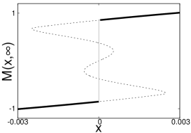
(4a) (4b) (4d)

Figure 3: Evolution of physical quantities by weak solution (NJL $g=1.7g_{\rm c}$,$~{}\mu=0.7$,$~{}t=0.01$, $0.5$, $0.6$, $\infty$). (a) Mass function. (b) Wilsonian fermion potential. (c) Legendre effective potential.

References

- (1) K-I. Aoki, Proc. SCGT96, 171 (1996):hep-ph/9706264, Prog. Theor. Phys. Suppl. 131, 129 (1998), Int. J. Mod. Phys. B 14, 1249 (2000).
- (2) K-I. Aoki, K. Morikawa, J.-I. Sumi, H. Terao and M. Tomoyose, Prog. Theor. Phys. 102, 1151 (1999), Phys. Rev. D 61, 045008 (2000).
- (3) H. Gies and C. Wetterich Phys. Rev. D 65, 065001 (2002).
- (4) K-I. Aoki and K. Miyashita Prog. Theor. Phys. 121, 875 (2009).
- (5) L. C. Evans, Partial Differential Equations, 2nd ed. (AMS, 2010).
- (6) K-I. Aoki and D. Sato Prog. Theor. Exp. Phys. 2013, 043B04 (2013).
- (7) K-I. Aoki and S.-I. Kumamoto and D. Sato in preparation.