Displacement induced electric force and natural self-oscillation of a free electron

Abstract

We show that a kind of displacement induced temporary electric force of a single point charge can be derived by using Maxwell stress analysis. This force comes from the variation of the charge’s electric intensities that follow Coulomb’s inverse square law, and it is a kind of displacement dependent temporary restoring force. We also show the possible existence of natural self-oscillation of a free electron which is driven by this restoring self-force of its own electric fields.

PACS numbers

03.50.De

I Introduction

The distance dependence of the electrostatic force of Coulomb’s inverse square law has been tested in high precision through different methods, see for example the discussion of JacksonJackson (1998) and experiment of Williams et alWilliams et al. (1971).

In this paper we want to show that some temporary displacement dependent electric force may be generated in relation to the Coulomb’s law. This is a kind of restoring electric self-force. It is induced by any displacement of the electric charge which changes the distribution of its electric fields that follow Coulomb’s law.

II The variation of distribution and magnitude of electric intensity of a charge subject to temporary displacement

For a particle with electric charge $e$ at rest at origin $O$ first, according to Coulomb’s law the distribution of its spherically symmetric electric intensity $E$ follows the inverse square law, that is

$${\bf E}={e\over r_{e}^{3}}{\bf{r}_{e}},$$ (1)

where $r_{e}$ is the magnitude of position vector from the particle to a field point. Suppose this charge is shifted along $z$ axis by a displacement $Z_{e}$ in a time interval $\triangle t$ and become stationary again at a position $O_{e}$. Thus the electromagnetic fields depending on its velocity and acceleration may be neglected first. By this displacement $Z_{e}$, the electric intensity $E$ of Eq. (1) will change in both magnitude and distribution. During this time interval any variation signal of the electromagnetic fields will propagate first from the origin $O$ to a spherical shell with radius $c\Delta{t}$ as shown in Fig. 1, where $c$ is velocity of light. At a position $P$ on this spherical shell, the distance to origin $O$ is the radius $r=c\Delta{t}$ and to the new origin $O_{e}$ is $[r_{e}]$. The relation between $[r_{e}]$ and $r=c\Delta t$ is that

$$[r_{e}]^{2}=(c\Delta{t})^{2}+Z_{e}^{2}-2c\Delta{t}{Z_{e}}\cos\theta,$$ (2)

where $\theta$ is the angle between $r$ and $z$ axis. Now the electric field outside this spherical shell does not change, the magnitude of the electric intensity on the outer boundary of this surface at $P$ is

$$E_{out}={e\over r^{2}}={e\over(c\Delta t)^{2}}.$$ (3)

The magnitude of the electric intensity on the inner boundary of this surface at $P$ is

$$E_{in}={e\over[r_{e}]^{2}}.$$ (4)

Since by Eq. (2) $[r_{e}]^{2}\neq(c\Delta t)^{2}$, these two electric intensities of Eq. (3) and Eq. (4) are not equal. But according to the requirement of div${\bf E}=0$ in charge free space, they should be equal in magnitude and direction. Although this requirement is applied for the total electric field, it is also correct for the Coulomb field alone here. Since $E_{out}$ of Eq. (3) is the primary value, it must remain unchanged, thus $E_{in}$ should be modified to fulfil the requirement of div${\bf E}=0$, that is to change $E_{in}$ to

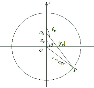
Figure 1: The relations between $r=c\Delta{t}$ and $[r_{e}]$.

$$E_{in}={e\over[r_{e}]^{2}}\cdot{[r_{e}]^{2}\over(c\Delta t)^{2}}={e\over{r_{e}}^{2}}MF={e\over(c\Delta t)^{2}},$$ (5)

where $MF$ is a kind of modification function. From Eq. (5) it is defined as

$$MF={[r_{e}]^{2}\over(c\Delta t)^{2}}=1+{Z_{e}^{2}\over(c\Delta t)^{2}}-{2Z_{e}\cos\theta\over c\Delta t}.$$ (6)

This kind of modification may also be seen from the relation of the solid angles $d\Omega$ and $d\Omega_{e}$ subtending to an area element $ds$ at position $P$ from the origins at $O$ and $O_{e}$ respectively as shown in Fig. 2. For the two solid angles we have

$$d\Omega={ds\over r^{2}}={ds\over(c\Delta t)^{2}},$$ (7)

$$d\Omega_{e}={ds\over[r_{e}]^{2}},$$ (8)

and following Eq. (6) we have

$${d\Omega\over d\Omega_{e}}={[r_{e}]^{2}\over r^{2}}={[r_{e}]^{2}\over(c\Delta t)^{2}}=MF.$$ (9)

Since the number of electric lines within solid angle $d\Omega_{e}$ should be the same as that within $d\Omega$, the area density of electric lines which represents the electric intensity will change by the ratio $MF$. This modification now not only modifies the electric intensity at position $P$, but should also be down to the whole solid angle $d{\Omega_{e}}$. Thus we may write the electric intensity within the solid angle $d{\Omega_{e}}$ as

$$E_{e}={e\over r_{e}^{2}}MF.$$ (10)

Then when the charge is subject to a temporary displacement $Z_{e}$ during time interval $\Delta t$, the electric intensities should be changed totally according to Eq. (10) within the spherical surface of radius $r=c\Delta t$.

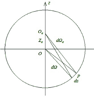
Figure 2: The relation between solid angles $d\Omega_{e}$ and $d\Omega$.

III Maxwell stress analysis of the displacement dependent electric force on a charge subject to a temporary displacement

It is known that electromagnetic force on a system may be calculated from the Maxwell stress on the surface that encloses this system. We see from above that for a particle with charge $e$ and subject to a temporary displacement $Z_{e}$, the distribution and magnitude of its electric intensity follows the modified Coulomb’s law as Eq. (10). Now we want to show that this particle will get a displacement dependent electric force generated by its own electric field, and this can be calculated from the Maxwell stress surrounding this particle. Now we may take a spherical surface with center at $O_{e}$ and radius $a$ surrounding this particle, and according to Eq. (10), the electric intensity at this surface $E_{a}$ as shown in Fig. 3 is

$$E_{a}={e\over a^{2}}MF.$$ (11)

According to the theory of Maxwell stress, the electric force on this particle may be calculated from the stress on the above-mentioned surface. For any electric intensity in space there is a corresponding Maxwell stress tensor $\bf T$ asJackson (1962)

$${\bf T}={1\over 4\pi}[{\bf EE}-{1\over 2}{\bf I}(E^{2})],$$ (12)

where $\bf I$ is the unit second rank tensor, the elements of $\bf T$ are

$$T_{ij}={1\over 4\pi}[E_{i}E_{j}-{1\over 2}I_{ij}E^{2}],$$ (13)

its force element $dF_{i}$ on an area element $ds$ at the surface is

$$dF_{i}=\sum_{j=1}^{3}T_{ij}ds_{j},$$ (14)

where $ds_{j}$ is the $j$ component of $ds$. The force $F_{i}$ on that surface is

$$F_{i}=\int dF_{i}.$$ (15)

On the spherical surface surrounding the charged particle, the distribution of electric intensity is Eq. (11) with directions along the normal of the surface element $ds$. Using Eqs. (13), (14) and (15), the total force along $z$ axis on the closed spherical surface is

$$F_{z} = \oint(T_{zz}ds_{z}+T_{zx}ds_{x}+T_{zy}ds_{y})$$ (16)

$$= \oint{1\over 4\pi}{1\over 2}(E_{z}^{2}-E_{x}^{2}-E_{y}^{2})ds_{z},$$

since the last two terms integrate to zero owing to their symmetry. Here $ds_{z}=a^{2}\sin{\theta_{e}}\cos{\theta_{e}}d\theta_{e}d\phi$ and we may take $\theta\approx\theta_{e}$ when $Z_{e}$ is small. Substituting $MF$ of Eq. (6) into Eq. (16) and using $E_{z}=E_{a}\cos{\theta_{e}}$, $E_{x}=E_{a}\sin{\theta_{e}}\cos{\phi}$ and $E_{y}=E_{a}\sin{\theta_{e}}\sin{\phi}$, we have

$$F_{z} = \displaystyle\oint{1\over 4\pi}{1\over 2}{e^{2}\over a^{4}}[1+{Z_{e}^{2}\over(c\Delta t)^{2}}-2{Z_{e}\cos\theta_{e}\over{c\Delta t}}]^{2}(\cos^{2}\theta_{e}-\sin^{2}\theta_{e}\cos^{2}\phi-\sin^{2}\theta_{e}\sin^{2}\phi)a^{2}\sin\theta_{e}\cos\theta_{e}d\theta_{e}d\phi$$ (17)

$$= \displaystyle\oint{e^{2}\over 4a^{2}}[1+{Z_{e}^{4}\over(c\Delta t)^{4}}+{4Z_{e}^{2}\cos^{2}\theta_{e}+2Z_{e}^{2}\over({c\Delta t})^{2}}-{4Z_{e}\cos\theta_{e}\over c\Delta t}-{4Z_{e}^{3}\cos\theta_{e}\over({c\Delta t})^{3}}](2\cos^{2}{\theta_{e}}-1)\cos{\theta_{e}}\sin{\theta_{e}}d\theta_{e}.$$

Here we integrate $\phi$ from 0 to $2\pi$. The odd terms of $\cos{\theta_{e}}$ integrate to zero. Since $Z_{e}$ is small, the important term of above integration is the first order term of $Z_{e}$, those higher order terms can be neglected, thus we have

$$F_{z}=\oint{e^{2}\over 4a^{2}}(-{4Z_{e}\cos\theta_{e}\over c{\Delta}t})(2\cos^{2}\theta_{e}-1)\cos\theta_{e}\sin\theta_{e}d\theta_{e},$$ (18)

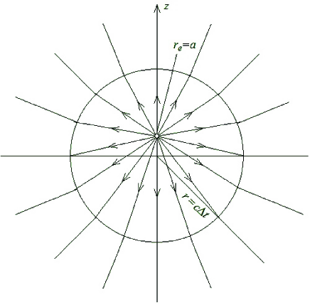
Figure 3: The distribution of electric intensities and electric field lines between two spherical surface with radii $r=c\Delta{t}$ and $r_{e}=a$.

thus

$$F_{z}=-{2e^{2}\over 15{a^{2}}}{Z_{e}\over c\Delta t}.$$ (19)

This displacement dependent $F_{z}$ is independent of the positive or negative sign of charge $e$ since it’s proportional to $e^{2}$. This is a kind of displacement dependent restore force induced by the variations of the charge’s own electric intensity which follows Coulomb’s inverse square law. The magnitude of this force is dependent on the radius $a$ of the spherical surface boundary of the charge. Here this force is also a temporary force. After the time interval $\Delta t$, as time goes on, $\Delta t$ increases to ${\Delta t}+t$, where $t$ is the additional time, then Eq. (19) will change to

$$F_{z}=-{2e^{2}\over 15{a^{2}}}{Z_{e}\over c({\Delta t}+t)}.$$ (20)

When $t$ becomes large, $F_{z}$ reduces to zero.

This problem cannot be treated by usual methods such as the time dependent Coulomb’s lawGriffiths and Heald (1991), the Lienard-Wiechart potentialPanofsky and Philips (1962) or the Feynman’s formulaFeynman et al. (1964) for a charge undergoing an arbitrary translation motion, since the variations of internal structure of the electric fields are not taken into account in these methods. Although the retarded time calculations are used in these methods, the historical conditions of the electric fields are ignored. The problem here is a kind of hereditary electromagnetismVolterra (1959). We do not use the integro-differential equation of functional analysis for this problem but the transit effect of displacement is treated in similar wayVolterra (1959). Similar analysis about the radiation of electric charge induced by its acceleration via the variation of electric field lines was given by othersOhanian (1980). Our discussions here emphasize only on the effect of displacement. The effect of velocity dependent magnetic fields is neglected and the equation of static cases is used as Eq. (14).

IV Possible effect of the displacement dependent restore force on the dynamics of a free electron

The displacement dependent restoring force of Eq. (19) is a kind of self-induced force. For a single free electron with charge $e$ and mass $m_{e}$ which is not subject to any external force, this self-induced force will affect its dynamical motion. We may take $M_{0}r_{0}$ as the radius $a$ above, where $M_{0}$ is an undetermined numerical constant, $r_{0}$ is the classical radius of electron which is defined asFeynman et al. (1964)

$$r_{0}={e^{2}\over m_{e}c^{2}}\approx 0.82\times 10^{-13}cm.$$ (21)

Substituting $M_{0}r_{0}$ into Eq. (19), we get

$$F_{z}=-{2e^{2}\over 15{(M_{0}r_{0})^{2}}}{Z_{e}\over c\Delta t}.$$ (22)

For an electron possessing self-sustained harmonic oscillation with angular frequency $\omega$, the time interval $\Delta t$ may be taken as $\pi/\omega$, which is half of its period. Then we have

$$F_{z}=-{2e^{2}\over 15{(M_{0}r_{0})^{2}}}{\omega Z_{e}\over c\pi}=-{2m_{e}c\omega{Z_{e}}\over 15{M_{0}^{2}}\pi{r_{0}}},$$ (23)

since $m_{e}={e^{2}/(r_{0}c^{2})}$ according to Eq. (21). If we take ${2c/(15M_{0}^{2}\pi{r_{0}})}=\omega$, then

$$F_{z}=-m_{e}\omega^{2}Z_{e},$$ (24)

which is a standard equation of harmonic oscillation of the free electron. This displacement dependent restore force implies that the electron may have a kind of natural self-oscillation as the “mono-electron oscillator” in a Penning trap of the experiment of Dehmelt et alWineland et al. (1973).

The oscillating electron will have oscillating static fields, velocity dependent and acceleration dependent fields, which may store energy and exchange energy between each otherMarion (1980); Mandel (1972). They need not always radiate out their energy through acceleration dependent electromagnetic fields if these fields have standing wave mode solutionsBateman (1955); Adler et al. (1960).

References

- Jackson (1998) J. D. Jackson, Classical Electrodynamics, 3rd ed. (John Wiley and Sons, 1998) p. 8.
- Williams et al. (1971) E. H. Williams, J. E. Faller, and H. A. Hill, Phys. Rev. Lett. 26, 721 (1971).
- Jackson (1962) J. D. Jackson, Classical Electrodynamics, 1st ed. (John Wiley and Sons, 1962) p. 193.
- Griffiths and Heald (1991) D. J. Griffiths and M. A. Heald, Am. J. Phys. 59, 111 (1991).
- Panofsky and Philips (1962) W. K. H. Panofsky and M. Philips, Classical Electricity and Magnetism (Addison-Wesley, 1962) Chap. 19, p. 341.
- Feynman et al. (1964) R. P. Feynman, R. B. Leighton, and M. Sands, The Feynman lectures on physics, Vol. 2 (Addison-Wesley, 1964) Chap. 21.
- Volterra (1959) V. Volterra, Theory of functionals and of integral and integro-differential equations (Addison-Wesley, 1959) Chap. VI, p. 194.
- Ohanian (1980) H. C. Ohanian, Am. J. Phys. 48, 170 (1980).
- Wineland et al. (1973) D. Wineland, P. Ekstorm, and H. Dehmelt, Phys. Rev. Lett. 31, 1279 (1973).
- Marion (1980) J. B. Marion, Classical Electromagnetic Radiation, 2nd ed. (Academic Press, 1980) Chap. 8, p. 285.
- Mandel (1972) L. Mandel, J. Opt. Soc. Am. 62, 1011 (1972).
- Bateman (1955) H. Bateman, The Mathematical Analysis of Electrical and Optical Wave Motion on the Basis of Maxwell’s Equations (Dover, 1955) Chap. 3, p. 36.
- Adler et al. (1960) R. B. Adler, L. J. Chu, and R. M. Fano, Electromagnetic Energy Transmission and Radiation (John Wiley and Sons, 1960) Chap. 10, p. 566.