Mesoscopic model for filament orientation in growing actin networks: the role of obstacle geometry

Abstract

Propulsion by growing actin networks is a universal mechanism used in many different biological systems, ranging from the sheet-like lamellipodium of crawling animal cells to the actin comet tails induced by certain bacteria and viruses in order to move within their host cells. Although the core molecular machinery for actin network growth is well preserved in all of these cases, the geometry of the propelled obstacle varies considerably. During recent years, filament orientation distribution has emerged as an important observable characterizing the structure and dynamical state of the growing network. Here we derive several continuum equations for the orientation distribution of filaments growing behind stiff obstacles of various shapes and validate the predicted steady state orientation patterns by stochastic computer simulations based on discrete filaments. We use an ordinary differential equation approach to demonstrate that for flat obstacles of finite size, two fundamentally different orientation patterns peaked at either $\pm 35$ or $+70/0/\!\!-\!\!70$ degrees exhibit mutually exclusive stability, in agreement with earlier results for flat obstacles of very large lateral extension. We calculate and validate phase diagrams as a function of model parameters and show how this approach can be extended to obstacles with piecewise straight contours. For curved obstacles, we arrive at a partial differential equation in the continuum limit, which again is in good agreement with the computer simulations. In all cases, we can identify the same two fundamentally different orientation patterns, but only within an appropriate reference frame, which is adjusted to the local orientation of the obstacle contour. Our results suggest that two fundamentally different network architectures compete with each other in growing actin networks, irrespective of obstacle geometry, and clarify how simulated and electron tomography data have to be analyzed for non-flat obstacle geometries.

I Introduction

The growth of actin networks is a generic propulsion mechanism occurring in a large variety of biological systems, ranging from the protruding lamellipodia of animal cells to the actin comet tails recruited by pathogens like the bacterium Listeria monocytogenes or the virus Vaccinia within their host cells. Due to its central importance, the molecular basis of this process is well preserved over a wide range of different species carlier2010 . Although a large number of accessory proteins is known to be involved in actin dynamics on the cellular scale, in regions close to the leading edge the dynamics of network growth are determined by a small number of key reactions. Here the interplay between three fundamental processes determines the structure of the growing network: polymerization of filamentous actin, branching mediated by the protein complex Arp2/3 and binding of capping proteins to the filament tip preventing further growth mullins1998 ; pollard2007 . The fact that these processes are highly conserved is impressively demonstrated by the observation that many intracellular pathogens rely on them for efficient infection and spread in the cytoplasm of their hosts frischknecht2001 ; gouin2005 ; lambrechts2008 . Even functionalized plastic beads, rods and discs as well as lipid vesicles and oil droplet in purified protein solutions containing this minimal set of molecules have been shown to be propelled in vitro by polymerizing actin networks loisel1999 ; cameron1999 ; upadhyaya2003 ; giardini2003 ; schwartz2004 ; boukellal2004 .

While the underlying molecular basis is very similar in all of these cases, the geometry of the different propelled objects is very different. For instance, the highly curved shape of relatively small, almost ellipsoidal pathogens like Listeria monocytogenes or Vaccinia virus is very different from the relatively flat shape of the leading edge of a crawling cells. The exact shape of the membrane in migrating cells is very dynamic, but certainly corrugated on different scales, thus in this case a flat obstacle shape can only be a first approximation and corrugated obstacle contours are also of large interest. In a growing actin network, new filaments nucleate by branching off from existing mother filaments at a characteristic angle around $70^{\circ}$ set by the molecular geometry of the Arp2/3-complex. Importantly, branching can occur only close to the surface, as it depends on the presence of surface-bound nucleation promoting factors (NPF) like WASP or ActA beltzner2008 . Whether the daughter filament becomes a productive member of the growing actin gel depends on the way its direction is oriented relative to the direction of growth and how the object is shaped. Therefore obstacle geometry is a crucial determinant of the resulting structural organization of the network.

One essential function of growing actin networks is to generate force against external load. Force-velocity relations for growing actin networks have been measured in different experimental setups and for various obstacle shapes wiesner2003 ; mcgrath2003 ; marcy2004 ; parekh2005 ; prass2006 ; heinemann2011 ; zimmermann2012 . Unexpected discrepancies in the results indicate that obstacle shape and the resulting difference in network organization also has an effect on force generation. Modern electron tomography leads to visualization and analysis of filamentous actin networks in ever greater detail resch2010 ; vinzenz2012 . While early electron microscopy data for the lamellipodia of fish keratocytes suggested a dendritic network of relatively short actin filaments svitkina1999 , recent electron tomography data has revealed a more diverse structural organization, with relatively long filaments connected by few branch points into different and spatially extended filament subsets urban2010 ; vinzenz2012 . In addition, it has been demonstrated that the structural organization of the network strongly depends on the protrusion speed, with fast growing networks dominated by two symmetric diagonal filament orientations and slowly growing networks featuring more filaments in parallel and orthogonal to the leading edge koestler2008 ; weichsel2012 . It is to be expected, that in the future the effect of obstacle geometry on network structure can be quantified by such methods as well.

In order to achieve a complete understanding of the structure of growing actin networks, different modeling approaches have been developed during the last decade carlsson2010_2 , ranging from microscopic ratchet models mogilner1996 ; mogilner2003 , rate equations for filament growth carlsson2003 ; maly2001 ; weichsel2010_2 and large-scale computer simulations of filament ensembles schaus2008 ; lee2009 ; alberts2004 ; schreiber2010 to continuum theories of how elastic stress propels the obstacle gerbal2000 and multi-scale models combining several of these model classes zimmermann2012 ; zhu2012 . From some of these studies it has emerged that one central quantity characterizing the structural organization of growing actin networks is the filament orientation distribution, which can be directly compared with experimental results maly2001 ; verkhovsky2003 ; schaub2007 ; weichsel2012 .

In the following, we study a model which allows us to predict the filament orientation distribution as a function of obstacle geometry. Our reference point will be stochastic computer simulations of growing actin networks incorporating the molecular processes of branching, capping and filament polymerization weichsel2010_2 . For computational simplicity and deeper insight, these will be compared to different versions of a rate equation model maly2001 ; carlsson2003 ; weichsel2010_2 . For actin growth behind flat and laterally widely spread obstacles the steady state organization has been predicted earlier to be either a $\pm 35$ or $+70/0/\!\!-\!\!70$ degree filament orientation pattern, with mutually exclusive stability determined by the model parameters maly2001 ; weichsel2010_2 . In this paper, we will extend this analysis to also predict the effect of finite size and geometry of the propelled object. In particular, we will derive and validate a partial differential equation, which is valid also for curved obstacle shapes.

The article is organized as follows: In Sec. II we introduce the model and explain how we analyze it. To validate our results, we compare different versions of a deterministic continuum model to stochastic computer simulations of filamentous networks. Subsequently, the impact of different piecewise straight (linear) obstacle shapes on the resulting network orientation patterns is analyzed in Sec. III, while specific examples for curved (nonlinear) obstacle shapes are the subject of Sec. IV. Our main result is that the competition between two fundamentally different network architectures persists for finite-sized, piecewise linear and curved obstacles.

II Model definition

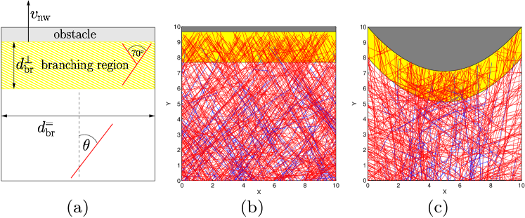
Figure 1: Model of a growing actin network behind a rigid obstacle. (a) Sketch of the setup. Branching can occur only in the yellow region. The main quantity of interest is the filament orientation angle $\theta$ relative to the surface normal. (b) Snapshot of a stochastic simulation based on the reactions of individual filaments for straight (linear) obstacle shape. (c) Snapshot of network growth behind a curved (nonlinear) obstacle shape. The network is growing in two dimensions. Red filaments are actively growing at their barbed end in direction $\theta$. Blue filaments have been capped and will eventually be outgrown by the network and leave the box at the bottom. Growth of the fastest filaments is stalled by the obstacle.

Motivated by established biological observations, in our model we assume Arp2/3 to nucleate daughter filaments from preexisting mother filaments at a characteristic relative branching angle around $70^{\circ}$ mullins1998 ; svitkina1999 ; ydenberg2011 . The exact value varies with biological system and analysis methods (for example, a recent value from electron tomography data for the lamellipodium of fibroblasts is $73\pm 8^{\circ}$ vinzenz2012 ), but is not essential for our theory. Although the exact mechanism for the activation of Arp2/3-mediated branching is not yet well established and subject of current research, it is generally accepted that Arp2/3 is active only near the obstacle, where it is activated by nucleation promoting factors (NPFs) such as the Wiskott–Aldrich syndrome protein (WASP) or the bacterial actin assembly-inducing protein (ActA) beltzner2008 ; ti2011 ; xu2012 . As we are interested in actin network architecture in close proximity to the surface of a propelled obstacle, we will focus on actin dynamics within the first few ten nanometers from the obstacle surface in which filament branching, capping and barbed end polymerization are expected to dominate actin dynamics, while filament depolymerization and decapping can be neglected schafer1996 . Fig. 1(a) sketches the geometrical arrangement studied here. The yellow branching region within a vertical distance $d_{\rm br}^{\perp}$ from the obstacle surface indicates the domain in which filament bound Arp2/3 is able to interact with NPFs, which themselves are active only close to the surface. Thus filament branching occurs in this branching region. Once filament barbed ends have left this domain due to their retrograde flow they are not able to nucleate new daughter filaments anymore and will eventually be outgrown by the bulk network. As those filaments subsequently do not impact the orientation distribution at the leading edge, we do not explicitly account for their further fate anymore. If the lateral extension $d_{\rm br}^{=}$ of the obstacle is large compared to the width $d_{\rm br}^{\perp}$ of the branching region, it is possible to neglect the process of filament barbed ends growing out of the branching region horizontally. However, for relatively small obstacles, for instance viral pathogens, the lateral dimension of the propelled particle $d_{\rm br}^{=}$ can become comparable to its vertical extension $d_{\rm br}^{\perp}$ and the finite lateral size of the branching region has to be taken into account. Our main quantity of interest is the filament orientation angle $\theta$ relative to the surface normal.

In the following, we will validate our theoretical approach by comparing results from two complementary implementations, namely stochastic computer simulations and a rate equation approach, which have been introduced before for flat obstacles of large lateral size weichsel2010_2 . Motivated by the flat nature of the lamellipodium and also for computational simplicity, our modeling is restricted to two dimensions. Representative snapshots of such simulations for flat and curved obstacle geometries are given in Fig. 1(b) and (c), respectively. Briefly, we simulate a network of infinitely stiff rods. This simplification is justified as the reaction kinetics that eventually determine the stable orientation distribution in steady state are active within a narrow branching region along the obstacle only. Because filament segments spanning over this region are very short compared to their persistence length (nanometers versus micrometers), local bending undulations are of minor importance here. The remainder of the filaments is considered to be entangled in the bulk actin network, which effectively acts as a base for the protruding filaments. However, filaments embedded in semidilute actin solutions have been found to exhibit substantial bending fluctuations in the past kaes1994 ; dichtl1999 and therefore we effectively account for a finite uncertainty in filament orientation by incorporating a distribution of relative branching angles between mother and daughter filaments in the model as is discussed below. Each uncapped filament is growing deterministically at its barbed end with a fixed velocity $v_{\rm fil}$. Thus we implicitly assume a constant density of actin monomers at the leading edge. Polymerization is quantized such that filaments extent by one building block of length $\delta_{\rm fil}$ per unit time. Apart from branching, individual filaments do not interact and hence the local filament density does not alter polymerization. Filament barbed ends within the branching region close to the leading edge are possible candidates for stochastic branching and capping events. While capping is assumed to be a first order reaction in the number of actin barbed ends in the reaction zone, for branching we assume zeroth order. This is motivated by the expectation that the supply of activated Arp2/3 is strongly limited by the availability of NPFs at the leading edge and thus an effective zeroth order branching rate emerges for sufficiently high filament density or low capping rate pollard2000 ; weichsel2012_2 . In the opposite limit of low filament density, the branching reaction is expected to become first order in the number of filaments; this effectively yields an autocatalytic description carlsson2003 , that is stationary only at one unique network growth velocity. Therefore in this limit, transitions in the filament orientation distribution are not accessible. However, it has been shown that both, first and zeroth order branching models, can be incorporated within a unified theoretical framework and that the crossover from one regime to the other does not have a direct impact on filament orientation in steady state weichsel2012_2 . As actin networks in most experimental setups are growing against a finite load of the obstacle and non-constant force-velocity curves are observed, the zeroth order branching regime is expected to dominate the branching kinetics eventually.

The orientation of new filament branches is chosen from a normalized linear combination of two Gaussian probability distributions for the angle between mother and daughter filament with means at $\pm 70^{\circ}$ and standard deviation $5^{\circ}$. Red filaments in the illustration are actively growing, while blue filaments indicate capped barbed ends that neither branch nor polymerize anymore and will eventually be outgrown by the bulk network and leave the simulation box at the bottom. In Fig. 1(b) the top boundary of the yellow branching region defines a rigid obstacle, which excludes volume and thus prevents polymerization above its boundary. As a consequence the fastest filaments which are growing in close to vertical direction are stalled by the obstacle. The vertical velocity of the obstacle is a parameter of the model and set to a constant value $v_{\rm nw}$ directly. This growth velocity should be regarded as the effective outcome in steady state, determined by the details of filament-obstacle interactions (including regulation by biochemical factors). Steady state growth is possible within the velocity range, $0<v_{\rm nw}<v_{\rm fil}$. Under these conditions a well defined filament number and orientation distribution evolves.

As a powerful analytical alternative to the stochastic framework introduced above, we also develop a deterministic rate equation for dendritic network growth based on earlier approaches of this kind maly2001 ; carlsson2003 ; weichsel2010_2 . The evolution of the orientation distribution $N(\theta,t)$ of uncapped filament barbed ends integrated over the whole branching region evolves in time by branching and capping events and by filaments growing out of the branching region. This translates into the following ordinary differential equation:

$$\frac{\partial N(\theta,t)}{\partial t}=\underbrace{\hat{k}_{\rm b}\int\mathcal{W}(\theta,\theta^{\prime})N(\theta^{\prime},t)\,\mbox{d}\theta^{\prime}}_{\text{branching}}-\underbrace{k_{\rm c}N(\theta,t)}_{\text{capping}}-\underbrace{k_{\rm gr}(\theta,v_{\rm nw})N(\theta,t)}_{\text{outgrowth}}\,.$$ (1)

Here again, capping is assumed to be a first order reaction proportional to the number of existing filaments with the proportionality constant, a reaction rate $k_{\rm c}$. The probability of branching at a given angle is determined by the weighting factor distribution, $\mathcal{W}(\theta,\theta^{\prime})$, which is modeled as a linear combination of Gaussians with maxima at branching angles $\pm 70^{\circ}$ between filaments and standard deviation $\sigma=5^{\circ}$. $\theta$ is the filament orientation angle measured relative to the vertical direction. The branching reaction is independent of the absolute number of existing filament barbed ends in this model (i.e. a zeroth order reaction). Hence, the branching rate $\hat{k}_{\rm b}$ is normalized by the total number of new filament ends,

$$\hat{k}_{\rm b}=\frac{k_{\rm b}}{\mathcal{W}_{\rm tot}}\ ,\ \mathcal{W}_{\rm tot}=\int\int\mathcal{W}(\theta,\theta^{\prime})N(\theta^{\prime},t)\,\mbox{d}\theta^{\prime}\,\mbox{d}\theta\,.$$ (2)

The reaction rate $k_{\rm b}$ indicates the number of new branches per unit time. Most importantly for the specific scope of this work, obstacle velocity and shape enter Eq. (1) via the outgrowth rate $k_{\rm gr}$. As filaments are polymerizing with a constant velocity $v_{\rm fil}$ in their individual direction, some filaments will not be able to keep up with the moving obstacle and thus leave the branching region. The precise expression for the rate of outgrowth $k_{\rm gr}$ strongly depends on obstacle geometry and alters the resulting steady state orientation distributions as will be analyzed in detail in the following.

III Linear obstacle shape

We begin our analysis with linear obstacle shapes as illustrated in Fig. 1(a) and (b). The obstacle (and therefore the leading edge of the network) moves with a constant velocity $v_{\rm nw}$ towards the top. Our region of interest, the branching region, extends vertically to a distance $d_{\rm br}^{\perp}$ from the leading edge of the network. The lateral obstacle width is indicated by $d_{\rm br}^{=}$.

III.1 Flat large obstacle

For obstacles that are laterally widely extended, for instance the leading edge at the front of the lamellipodium in a migrating cell, we have $d_{\rm br}^{=}\gg d_{\rm br}^{\perp}$ and thus horizontal filament outgrowth can be neglected locally. Mathematically, this means that we can use periodic boundary conditions in the horizontal direction. This case has been analyzed before in a similar manner as done below for finite-sized and curved obstacles weichsel2010_2 , and therefore we recapitulate the most important results as a reference case. In this simple case, outgrowth of filaments from the branching region can only occur in negative normal direction. While the network grows with velocity $v_{\rm nw}$ in positive normal direction, single filaments grow with velocity $v_{\rm fil}$ in their individual direction. The projected polymerization velocity depends on the filament orientation, as

$$v_{\rm fil}^{\perp}(\theta)=v_{\rm fil}\cos\theta\,.$$ (3)

Filaments having a larger absolute orientation than the critical angle

$$\theta_{\rm c}=\arccos\left(\frac{v_{\rm nw}}{v_{\rm fil}}\right)\,,$$ (4)

are thus not able to keep up with the speed of the obstacle and are subject to outgrowth with a rate

$${k_{\rm gr}^{\perp}}(\theta,v_{\rm nw})=\begin{cases}0&\text{if $|\theta|\leq\theta_{\rm c}$}\\ \frac{v_{\rm nw}-v_{\rm fil}\cos{\theta}}{(d_{\rm br}^{\perp}/2)}&\text{if $|\theta|>\theta_{\rm c}$}\end{cases}\ .$$ (5)

The factor $2$ results from the assumption that new filaments branch-off from existing filaments on average in the center of the branching region of vertical width $d_{\rm br}^{\perp}$. Outgrowth vanishes for filaments with an orientation smaller than a critical angle $\theta_{\rm c}$ and from there increases to its maximum at $|\theta|=180^{\circ}$.

We solve Eq. (1) numerically by introducing 360 angle bins and iterating the equations until a steady state is achieved, which then can be compared to the results of the stochastic computer simulations. In order to achieve a deeper understanding, we also introduced a coarse-grained version of Eq. (1) that can be treated analytically. In Eq. (1), the number of filament ends in the branching region with angles between $\theta$ and $\theta+d\theta$ is given by $N(\theta,t)d\theta$. By extending this integration to sufficiently large ($\Delta\theta=35^{\circ}$) angle bins

$$N_{\bar{\theta}}=\int\limits_{\bar{\theta}-\Delta\theta/2}^{\bar{\theta}+\Delta\theta/2}N(\theta^{\prime},t)\,\mbox{d}\theta^{\prime}\,,$$ (6)

and further assuming that branching is restricted to pairs of angle bins with a relative angle difference of $70^{\circ}$, a system of five coupled ordinary differential equations results:

$$\frac{\partial N_{-70^{\circ}}}{\partial t} = \frac{1}{2}\hat{k}_{\rm b}N_{0^{\circ}}-\left(k_{\rm c}+{k_{\rm gr}^{\perp}}(70^{\circ})\right)N_{-70^{\circ}}$$ (7)

$$\frac{\partial N_{-35^{\circ}}}{\partial t} = \frac{1}{2}\hat{k}_{\rm b}N_{+35^{\circ}}-\left(k_{\rm c}+{k_{\rm gr}^{\perp}}(35^{\circ})\right)N_{-35^{\circ}}$$ (8)

$$\frac{\partial N_{0^{\circ}}}{\partial t} = \frac{1}{2}\hat{k}_{\rm b}\left(N_{-70^{\circ}}+N_{+70^{\circ}}\right)-k_{\rm c}N_{0^{\circ}}$$ (9)

$$\frac{\partial N_{+35^{\circ}}}{\partial t} = \frac{1}{2}\hat{k}_{\rm b}N_{-35^{\circ}}-\left(k_{\rm c}+{k_{\rm gr}^{\perp}}(35^{\circ})\right)N_{+35^{\circ}}$$ (10)

$$\frac{\partial N_{+70^{\circ}}}{\partial t} = \frac{1}{2}\hat{k}_{\rm b}N_{0^{\circ}}-\left(k_{\rm c}+{k_{\rm gr}^{\perp}}(70^{\circ})\right)N_{+70^{\circ}}\,,$$ (11)

with

$$\hat{k}_{\rm b}=\frac{k_{\rm b}}{\mathcal{W}_{\rm tot}}=\frac{k_{\rm b}}{N_{-70^{\circ}}+N_{-35^{\circ}}+N_{0^{\circ}}+N_{+35^{\circ}}+N_{+70^{\circ}}}\,.$$

Here we have also assumed that branching of filaments with orientations $|\theta|>87.5^{\circ}$ can be neglected. The five equations are symmetric around $0^{\circ}$, and thus only three of them are independent. Nonlinearity and the coupling of all five equations is introduced by the branching term due to the zeroth order branching reaction.

By algebraically solving Eq. (7))–(Eq. (11) for the stationary state, we obtain two physically meaningful solutions. The first solution,

$$\begin{array}[]{rcl}N_{-70^{\circ}}^{\rm ss35}&=&0\\ N_{-35^{\circ}}^{\rm ss35}&=&k_{\rm b}\frac{1}{4(k_{\rm c}+{k_{\rm gr}^{\perp}}(35^{\circ}))}\\ N_{0^{\circ}}^{\rm ss35}&=&0\\ N_{+35^{\circ}}^{\rm ss35}&=&k_{\rm b}\frac{1}{4(k_{\rm c}+{k_{\rm gr}^{\perp}}(35^{\circ}))}\\ N_{+70^{\circ}}^{\rm ss35}&=&0\,,\end{array}$$ (17)

represents a dominant $\pm 35$ degrees orientation distribution in the steady state while the second solution,

$$\begin{array}[]{rcl}N_{-70^{\circ}}^{\rm ss70}&=&k_{\rm b}\frac{k_{\rm c}+{k_{\rm gr}^{\perp}}(70^{\circ})-\sqrt{2k_{\rm c}\left(k_{\rm c}+{k_{\rm gr}^{\perp}}(70^{\circ})\right)}}{2\left({k_{\rm gr}^{\perp}}^{2}(70^{\circ})-k_{\rm c}^{2}\right)}\\ N_{-35^{\circ}}^{\rm ss70}&=&0\\ N_{0^{\circ}}^{\rm ss70}&=&k_{\rm b}\frac{1-\sqrt{\frac{k_{\rm c}+{k_{\rm gr}^{\perp}}(70^{\circ})}{2k_{\rm c}}}}{k_{\rm c}-{k_{\rm gr}^{\perp}}(70^{\circ})}\\ N_{+35^{\circ}}^{\rm ss70}&=&0\\ N_{+70^{\circ}}^{\rm ss70}&=&k_{\rm b}\frac{k_{\rm c}+{k_{\rm gr}^{\perp}}(70^{\circ})-\sqrt{2k_{\rm c}\left(k_{\rm c}+{k_{\rm gr}^{\perp}}(70^{\circ})\right)}}{2\left({k_{\rm gr}^{\perp}}^{2}(70^{\circ})-k_{\rm c}^{2}\right)}\,,\end{array}$$ (23)

corresponds to a competing $+70/0/\!\!-\!\!70$ pattern.

The stability of these two fixed points can be analyzed with respect to the parameters $k_{\rm b}$, $k_{\rm c}$, $k_{\rm gr}^{\perp}(35^{\circ})$, ${k_{\rm gr}^{\perp}}(70^{\circ})$ and $d_{\rm br}^{\perp}$ using linear stability analysis. The result of this analysis is independent of the branching rate $k_{\rm b}$ and therefore this parameter has no influence on the stability of the system. According to Eq. (17) and Eq. (23), however, the total number of filaments in steady state is proportional to $k_{\rm b}$ and therefore this parameter can be used to adjust the model to experimentally measured densities. The two parameters ${k_{\rm gr}^{\perp}}(35^{\circ})$ and $k_{\rm gr}^{\perp}(70^{\circ})$ are not independent, but rather both of them are determined by the obstacle velocity $v_{\rm nw}$ as given in Eq. (5). In the following, we will omit the ill-defined cases $k_{\rm c}={k_{\rm gr}^{\perp}}(35^{\circ})=0$ and $k_{\rm c}={k_{\rm gr}^{\perp}}(70^{\circ})=0$, for which the filament number diverges. We find that the stability of both fixed points changes when

$$k_{\rm c}{k_{\rm gr}^{\perp}}(70^{\circ})=k_{\rm c}^{2}+4k_{\rm c}{k_{\rm gr}^{\perp}}(35^{\circ})+2{k_{\rm gr}^{\perp}}^{2}(35^{\circ})$$ (24)

and that either one is asymptotically stable, while the other is a saddle. Thus the simple model suggests that exactly two possible network architectures exist with mutually exclusive stability.

Eq. (24) can now be used to obtain the respective network velocity $v_{\rm nw}$ of the transition. For a critical angle $\theta_{\rm c}\geq 70^{\circ}$ (i.e. $k_{\rm gr}^{\perp}(70^{\circ})={k_{\rm gr}^{\perp}}(35^{\circ})=0$), Eq. (24) is never satisfied (note that $k_{\rm c}>0$). For $35^{\circ}\leq\theta_{\rm c}<70^{\circ}$ (i.e. ${k_{\rm gr}^{\perp}}(70^{\circ})>0\wedge{k_{\rm gr}^{\perp}}(35^{\circ})=0$),

$$v_{\rm nw}=\frac{1}{2}k_{\rm c}d_{\rm br}^{\perp}+v_{\rm fil}\cos(70^{\circ})\,\textnormal{, for }35^{\circ}\leq\theta_{\rm c}<70^{\circ}\ .$$ (25)

satisfies Eq. (24). For network velocities with a critical angle $\theta_{\rm c}<35^{\circ}$ (i.e. ${k_{\rm gr}^{\perp}}(70^{\circ})>{k_{\rm gr}^{\perp}}(35^{\circ})>0$), two solutions emerge,

$$\begin{array}[]{rcl}v_{\rm nw\,1,2}&=&\frac{1}{8}\left(-3k_{\rm c}d_{\rm br}^{\perp}+8v_{\rm fil}\cos(35^{\circ})\right)\\ &&\pm\frac{1}{8}\sqrt{k_{\rm c}d_{\rm br}^{\perp}\left(k_{\rm c}d_{\rm br}^{\perp}+16v_{\rm fil}\cos(35^{\circ})-16v_{\rm fil}\cos(70^{\circ})\right)}\,,\\ &&\textnormal{for }\theta_{\rm c}<35^{\circ}\,.\\ \end{array}$$ (29)

It turns out that solution Eq. (25) is valid for network bulk velocities $v_{\rm fil}\cos(35^{\circ})\geq v_{\rm nw}>v_{\rm fil}\cos(70^{\circ})$, while for solution Eq. (29) to be valid $v_{\rm nw}>v_{\rm fil}\cos(35^{\circ})$ has to be satisfied. This is never the case for the negative square-root in Eq. (29) and so we can neglect this solution in the following. In order to further simplify our equations, we define the reference velocity $u_{\rm c}\equiv k_{\rm c}d_{\rm br}^{\perp}$ resulting from the capping rate. Eq. (25) and Eq. (29) then become

$$\frac{v_{\rm nw}}{v_{\rm fil}}=\frac{1}{2}\frac{u_{\rm c}}{v_{\rm fil}}+\cos(70^{\circ})\,,$$ (30)

and,

$$\begin{array}[]{rcl}\frac{v_{\rm nw}}{v_{\rm fil}}&=&\frac{1}{8}\left(-3\frac{u_{\rm c}}{v_{\rm fil}}+8\cos(35^{\circ})\right)\\ &&+\frac{1}{8}\sqrt{\frac{u_{\rm c}}{v_{\rm fil}}\left(\frac{u_{\rm c}}{v_{\rm fil}}+16\cos(35^{\circ})-16\cos(70^{\circ})\right)}\,,\end{array}$$ (33)

respectively. Thus the capping rate emerges as an essential parameter through the effective velocity $u_{\rm c}$.

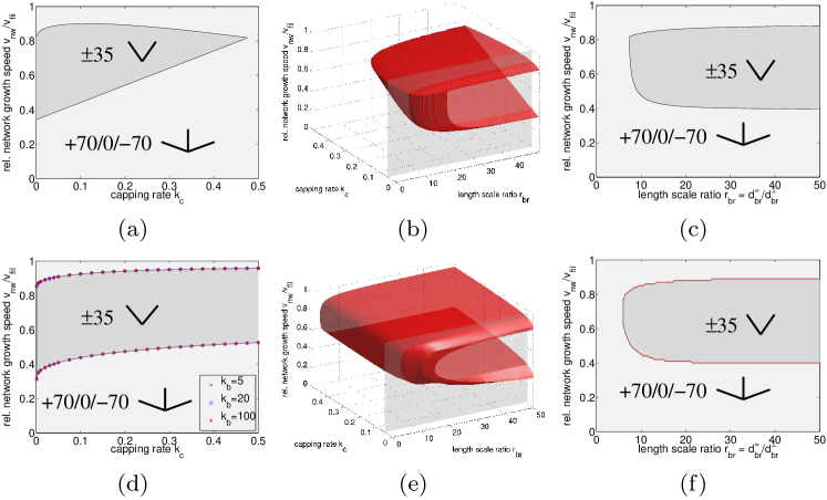
Figure 2: Phase diagram for flat finite-sized obstacles. (a-c) Analytical results from linear stability analysis of the simplified continuum model with 5 angle bins. (d-f) Full numerical solution of the rate equation model with $360$ angle bins. In (a) and (d), 2D slices through the 3D hypersurface are plotted within the $k_{\rm c}$-$v_{\rm nw}$ plane in the limit of $r_{\rm br}\rightarrow\infty$, which corresponds to periodic boundary conditions or very large objects. (b) and (e) show the hyperplane of transition points between the two filament patterns in the full 3D parameter space. In (c) and (f), slice plots in the $r_{\rm br}$-$v_{\rm nw}$ plane are shown along the transparent gray plane in (b) and (e) at $k_{\rm c}=0.05$.

In Fig. 2(a) the stability diagram from the analytical analysis is illustrated, showing the regions in which either the $\pm 35$ degree distribution is asymptotically stable and the $+70/0/\!\!-\!\!70$ pattern is a saddle or vice versa. In order to compare these results to the full numerical solution of Eq. (1), we define the relative difference of filaments in the angle bin around $0^{\circ}$ to the one around $35^{\circ}$ as an appropriate order parameter in steady state,

$$\mathcal{O}=\frac{N_{0^{\circ}}-N_{35^{\circ}}}{N_{0^{\circ}}+N_{35^{\circ}}}=\left[-1,+1\right]\,.$$ (34)

For a perfect $+70/0/\!\!-\!\!70$ distribution this parameter will approach $+1$, while for the competing $\pm 35$ pattern it will approach $-1$. The transition between the two patterns is defined when the order parameter changes its sign. According to this definition of the transition point, it is now possible to numerically solve the continuum model Eq. (1) and to classify each observed stationary state as one of the two phases. These results are presented as a phase diagram in Fig. 2(d) and were obtained for different branching rates $k_{\rm b}$, which indeed has no significant influence as expected from the analytical considerations. In the solution of the full continuum model the capping rate only has a very limited influence on the stripe-like pattern of the phase diagram. Contrarily, in the phase diagram resulting from linear stability analysis (Fig. 2(a)), the $\pm 35$ pattern vanishes at large capping rate. This artifact of the reduced rate equation model is introduced by the assumption that filaments with an orientation larger than $87.5^{\circ}$ do not branch. As the full rate equation does not share this assumption, it does not predict the elimination of the $\pm 35$ pattern for large capping rate.

III.2 Flat finite-sized obstacle

For flat, but finite-sized obstacle shape, filaments might also leave the branching region horizontally. Therefore a second outgrowth rate needs to be incorporated into the rate equation (Eq. (1)):

$$k_{\rm gr}^{=}(\theta,v_{\rm nw})=\begin{cases}\frac{v_{\rm nw}\tan{\theta}}{(d_{\rm br}^{=}/2)}&\text{if $|\theta|\leq\theta_{\rm c}$}\\ \frac{v_{\rm fil}\sin{\theta}}{(d_{\rm br}^{=}/2)}&\text{if $|\theta|>\theta_{\rm c}$}\end{cases}\,.$$ (35)

We find that for this scenario, it is still possible to analyze the stability of the fixed points of Eq. (7)–Eq. (11). The only difference that accounts for the change in obstacle geometry at this point is that a combination of outgrowth rates $k_{\rm gr}(\theta)=k_{\rm gr}^{\perp}(\theta)+|k_{\rm gr}^{=}(\theta)|$ replaces the term for exclusively orthogonal outgrowth $k_{\rm gr}^{\perp}(\theta)$ considered in the previous section. For filaments growing in the $N_{0^{\circ}}$ angle bin, both outgrowth rates vanish, because these filaments are growing at a high enough velocity parallel to the lateral boundaries of the obstacle.

The same arguments as used before also apply for the stability analysis of the steady states here. Hence, we can begin with Eq. (24) and evaluate the stability of the two steady states according to the adjusted outgrowth rate. To determine the transitions, we will follow a similar strategy as before. Starting from small network velocities $v_{\rm nw}$, we will treat the different possibilities for the outgrowth rates given in Eq. (5) and Eq. (35) in a case-by-case analysis.

For $\theta_{\rm c}\geq 70^{\circ}$, the orthogonal outgrowth rates vanish, as all relevant filament orientations grow faster towards the top than the obstacle and are slowed down to $v_{\rm nw}$ in this direction. The outgrowth rates for the different orientation bins therefore read,

$$k_{\rm gr}^{\perp}(\theta)=0\text{ and }k_{\rm gr}^{=}(\theta)=\frac{v_{\rm nw}\tan{\theta}}{(d_{\rm br}^{=}/2)}\text{ for }\theta=[35^{\circ},70^{\circ}]\,.$$ (36)

Inserting $k_{\rm gr}=k_{\rm gr}^{\perp}+k_{\rm gr}^{=}$ in Eq. (24) and omitting again the ill-defined cases of $k_{\rm b}=0$, $k_{\rm c}=0$ and $d_{\rm br}^{=}=0$ here (and additionally $d_{\rm br}^{\perp}=0$ in the following), it can be shown that Eq. (24) is never satisfied.

Increasing the network velocity to the point where $35^{\circ}\leq\theta_{\rm c}<70^{\circ}$ leads to outgrowth rates,

$$k_{\rm gr}^{\perp}(35^{\circ})=0\text{ and }k_{\rm gr}^{\perp}(70^{\circ})=\frac{v_{\rm nw}-v_{\rm fil}\cos(70^{\circ})}{(d_{\rm br}^{\perp}/2)}\,,$$ (37)

in orthogonal direction according to Eq. (5) and,

$$k_{\rm gr}^{=}(35^{\circ})=\frac{v_{\rm nw}\tan(35^{\circ})}{(d_{\rm br}^{=}/2)}\text{ and }k_{\rm gr}^{=}(70^{\circ})=\frac{v_{\rm fil}\sin(70^{\circ})}{(d_{\rm br}^{=}/2)}\,,$$ (38)

in the lateral direction according to Eq. (35). These rates yield a quadratic equation for the network velocities $v_{\rm nw}$ that satisfy Eq. (24),

$$\begin{array}[]{rcl}0&=&v_{\rm nw}^{2}\left[8\tan^{2}(35^{\circ})\frac{1}{{u_{\rm c}}^{2}{r_{\rm br}}^{2}}\right]+v_{\rm nw}\left[8\tan(35^{\circ})\frac{1}{u_{\rm c}r_{\rm br}}-2\frac{1}{u_{\rm c}}\right]\\ &&+\left[1-2v_{\rm fil}\sin(70^{\circ})\frac{1}{u_{\rm c}r_{\rm br}}+2v_{\rm fil}\cos(70^{\circ})\frac{1}{u_{\rm c}}\right]\,,\\ &&\textnormal{for }35^{\circ}\leq\theta_{\rm c}<70^{\circ}\,.\end{array}$$ (39)

Here, the reference velocity, $u_{\rm c}=k_{\rm c}d_{\rm br}^{\perp}$, together with a new parameter for the length scale ratio in lateral and orthogonal direction, $r_{\rm br}\equiv d_{\rm br}^{=}/d_{\rm br}^{\perp}$, are identified to determine stability.

For a critical angle $\theta_{\rm c}<35^{\circ}$, the adjusted outgrowth rates read,

$$k_{\rm gr}^{\perp}(\theta)=\frac{v_{\rm nw}-v_{\rm fil}\cos{\theta}}{(d_{\rm br}^{\perp}/2)}\text{ and }k_{\rm gr}^{=}(\theta)=\frac{v_{\rm fil}\sin{\theta}}{(d_{\rm br}^{=}/2)}\text{ for }\theta=[35^{\circ},70^{\circ}]\,.$$ (40)

These rates together with Eq. (24) and the effective parameters $u_{\rm c}$ and $r_{\rm br}$ can be simplified to a second quadratic equation defining the network velocities at the transitions,

$$\begin{array}[]{rcl}0&=&v_{\rm nw}^{2}\left[8\frac{1}{u_{\rm c}^{2}}\right]+v_{\rm nw}\left[6\frac{1}{u_{\rm c}}-16v_{\rm fil}\cos(35^{\circ})\frac{1}{u_{\rm c}^{2}}+16v_{\rm fil}\sin(35^{\circ})\frac{1}{u_{\rm c}^{2}r_{\rm br}}\right]\\ &&+\left[1+2v_{\rm fil}\cos(70^{\circ})\frac{1}{u_{\rm c}}-2v_{\rm fil}\sin(70^{\circ})\frac{1}{u_{\rm c}r_{\rm br}}-8v_{\rm fil}\cos(35^{\circ})\frac{1}{u_{\rm c}}+8v_{\rm fil}\sin(35^{\circ})\frac{1}{u_{\rm c}r_{\rm br}}\right.\\ &&\hskip 14.22636pt+\left.8v_{\rm fil}^{2}\cos^{2}(35^{\circ})\frac{1}{u_{\rm c}^{2}}-16v_{\rm fil}^{2}\cos(35^{\circ})\sin(35^{\circ})\frac{1}{u_{\rm c}^{2}r_{\rm br}}+8v_{\rm fil}^{2}\sin^{2}(35^{\circ})\frac{1}{u_{\rm c}^{2}r_{\rm br}^{2}}\right]\,,\\ &&\textnormal{for }\theta_{\rm c}<35^{\circ}\,.\end{array}$$ (41)

According to Eq. (39) and Eq. (41), the regions of stability for the two different stationary orientation patterns in parameter space are illustrated in Fig. 2(b). As the finite obstacle width introduces an additional independent parameter $r_{\rm br}$, the full parameter space is now three dimensional. Network growth velocities $v_{\rm nw}$ that fulfill Eq. (39) together with the condition $v_{\rm fil}\cos(35^{\circ})\geq v_{\rm nw}>v_{\rm fil}\cos(70^{\circ})$ or Eq. (41) at $v_{\rm nw}>v_{\rm fil}\cos(35^{\circ})$ are identified as transition points between the different orientation distributions in the parameter space spanned by $k_{\rm c}$, $r_{\rm br}$ and $v_{\rm nw}$. In the limit of large length scale ratio, $r_{\rm br}\rightarrow\infty$ (i.e. $d_{\rm br}^{=}\gg d_{\rm br}^{\perp}$), lateral outgrowth can be neglected and the phase diagram approaches the results for periodic boundary conditions as given in Fig. 2(a). For relatively small $r_{\rm br}\lesssim 7$, the lateral outgrowth of intermediate filament orientations at around $\pm 35^{\circ}$ is sufficiently large to prevent this orientation pattern from being stable in this model, independent of the growth velocity (cf. Fig. 2(c)).

Using the order parameter Eq. (34), we numerically sampled the parameter space according to Eq. (1) with adjusted outgrowth. The isosurface $\mathcal{O}(v_{\rm nw},k_{\rm c},r_{\rm br})=0$ is extracted from the three dimensional data and shown in Fig. 2(e). In the limit of large length scale ratio, the results coincide well with the case of periodic boundary conditions (cf. Fig. 2(d)). It is also confirmed that for small values of $r_{\rm br}$ the $\pm 35$ pattern is not stable anymore at intermediate velocities (cf. Fig. 2(f)). Thus the overall agreement between the simple analytical model and the full numerical solution of the rate equation approach is surprisingly good.

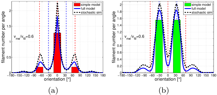
Figure 3: Comparison of the steady state orientation distributions for actin networks growing in the tail of a flat obstacle of finite size at $v_{\rm nw}/v_{\rm fil}=0.6$, $k_{\rm b}=20$, $k_{\rm c}=0.05$, $d_{\rm br}^{\perp}=2\delta_{\rm fil}$ and (a) $r_{\rm br}=3$, (b) $r_{\rm br}=20$. The results were obtained according to three different methods, the simplified continuum model (bars), the full continuum model (blue solid line) and stochastic simulations (black dashed line).

Fig. 3 compares filament orientation distributions obtained in steady state from stochastic network simulations, the full continuum model and the simplified continuum model. The parameters of the two cases shown in (a) and (b) do not differ in their network velocity $v_{\rm nw}$, but rather only in the obstacle geometry, in this case given by length scale ratio $r_{\rm br}=d_{\rm br}^{=}/d_{\rm br}^{\perp}$. For small $r_{\rm br}=3$ at intermediate velocities, the $\pm 35$ pattern of the network is not stable anymore and rather the network organizes in the alternative $+70/0/\!\!-\!\!70$ distribution (cf. Fig. 3(a)). For larger ratio $r_{\rm br}=20$, the network organizes in the $\pm 35$ degree distribution (cf. Fig. 3(b)). In the stochastic simulations, outgrowth rates are not explicitly incorporated, but rather emerge as a direct consequence of the obstacle geometry. Thus the computer simulations nicely validate both, the full and reduced continuum approaches, and all three seem to capture the essential physical mechanisms determining network structure.

III.3 Obstacle with tilted straight contour

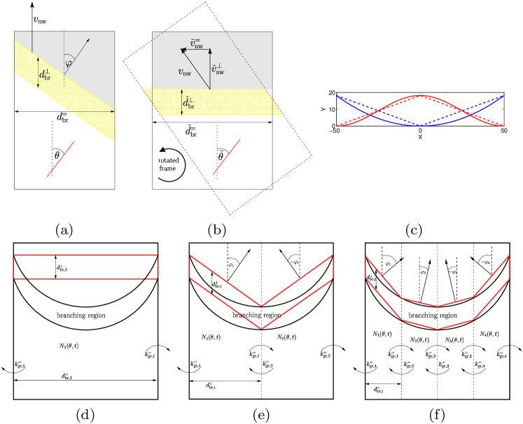
Figure 4: (a) and (b) Within a rotated coordinate frame, the continuum model (Eq. (1)) is applicable to treat filament networks growing behind a skewed linear obstacle. (a) Lab frame: A generic skewed linear obstacle with skew angle $\varphi$. (b) Obstacle frame: The coordinate system is rotated by its skew angle $\varphi$ counter-clockwise. In this frame the initial skew of the system is expressed by an additional finite lateral motion at velocity $\tilde{v}_{\rm nw}^{=}$ of an otherwise flat obstacle moving at $\tilde{v}_{\rm nw}^{\perp}$. (c) Parabolic (blue) and cosine (red) nonlinear obstacle shapes. The solid lines indicate the nonlinear obstacle shape, while the dashed line corresponds to a piecewise-linear triangular approximation. Horizontally the parabolic shape has a finite width, while the cosine obstacle shape is analyzed in periodic conditions laterally. (d-f) Piecewise-linear approximations of a parabola-like obstacle geometry. (d) The simplest approximation is a flat linear obstacle. (e) Due to the left-right symmetry in obstacle shape, in higher order approximations of the nonlinear obstacle (e.g. the triangular approximation shown here), only half of the number of sections have to be considered explicitly. The boundary condition at the center of the box has to be adjusted accordingly. (f) Subdividing the piecewise-linear sections again and again leads to ever higher accuracy in the approximation of the nonlinear obstacle shape and to ever smaller horizontal width of each subsection, $d_{{\rm br},i}^{=}=d_{\rm br}^{=}/n$. Approaching the continuum limit, $n\rightarrow\infty$, yields a PDE-model for nonlinear obstacle shapes.

It is not trivial to find an explicit expression for the outgrowth rate out of the branching region behind a skewed linear obstacle, which is rotated according to a constant skew angle $\varphi$, with $-90^{\circ}<\varphi<+90^{\circ}$. However, for reasonably small skew angle $\varphi$ and width of the orthogonal branching region $d_{\rm br}^{\perp}$ an approximation can be obtained within a rotated coordinate frame, that is adjusted to the constant obstacle skew. Fig. 4(a) shows a sketch of the obstacle geometry we are interested in at this point. The branching region is given by a rhomboid, with rotated (or skewed) upper and lower side. The orthogonal width of the branching region $d_{\rm br}^{\perp}$ is again defined parallel to the lateral sides of the obstacle, while its horizontal width is given by $d_{\rm br}^{=}$. Network velocity $v_{\rm nw}$ is defined as before in the vertical direction. To find an explicit expression for the rates of filament outgrowth, a rotation of the coordinate frame to the point where the skew angle $\varphi$ of the branching region vanishes simplifies the situation (Fig. 4(b)). In this frame the obstacle appears flat horizontally, very similar to the setup analyzed before in Sec. III.2. The finite skew angle $\varphi$, however, manifests in a non-vanishing lateral network growth velocity $\tilde{v}_{\rm nw}^{=}$, while the vertical propulsion speed of the obstacle is the orthogonal part of the network velocity in this frame, $\tilde{v}_{\rm nw}^{\perp}$. (Where applicable, we will denote variables defined in the rotated coordinate frame by $\,\tilde{}\,$.) In the following we will refer to the original coordinate system Fig. 4(a) as the lab frame and to the rotated picture Fig. 4(b) as the obstacle frame.

Using the transformation to the obstacle frame for a given skew angle $\varphi$, we can now deduce the relevant parameters. The filament orientation angles $\tilde{\theta}$ are given relative to the obstacle, i.e. for $\tilde{\theta}=0^{\circ}$ filaments are growing vertically in the rotated frame. The two components of obstacle growth velocity are given by,

$$\tilde{v}_{\rm nw}^{\perp}(\varphi)=v_{\rm nw}\cos\varphi\textnormal{ and }\tilde{v}_{\rm nw}^{=}(\varphi)=v_{\rm nw}\sin\varphi\,.$$ (42)

The two obstacle diameters, which scale the vertical and horizontal outgrowth rates are,

$$\tilde{d}_{\rm br}^{\perp}(\varphi)=d_{\rm br}^{\perp}\cos\varphi\textnormal{ and }\tilde{d}_{\rm br}^{=}(\varphi)=\frac{d_{\rm br}^{=}}{\cos\varphi}\,.$$ (43)

According to these definitions, we can now reformulate the continuum description in the obstacle frame. The rate equation model Eq. (1) for the temporal evolution of orientation dependent filament density remains unchanged with respect to the transformed orientation angles $\tilde{\theta}$, however with adjusted outgrowth rate $k_{\rm gr}(\theta,v_{\rm nw})$ given by the sum of orthogonal outgrowth,

$${\tilde{k}_{\rm gr}^{\perp}}(\tilde{\theta},\varphi,v_{\rm nw})=\begin{cases}0&\text{if $|\tilde{\theta}|\leq\tilde{\theta}_{\rm c}$}\\ \frac{\tilde{v}_{\rm nw}^{\perp}(\varphi)-v_{\rm fil}\cos{\tilde{\theta}}}{(\tilde{d}_{\rm br}^{\perp}(\varphi)/2)}&\text{if $|\tilde{\theta}|>\tilde{\theta}_{\rm c}$}\end{cases}\,,$$ (44)

and the absolute value of lateral outgrowth,

$${\tilde{k}_{\rm gr}^{=}}(\tilde{\theta},\varphi,v_{\rm nw})=\begin{cases}\frac{\tilde{v}_{\rm nw}^{=}(\varphi)+\tilde{v}_{\rm nw}^{\perp}(\varphi)\tan{\tilde{\theta}}}{(\tilde{d}_{\rm br}^{=}(\varphi)/2)}&\text{if $|\tilde{\theta}|\leq\tilde{\theta}_{\rm c}$}\\ \frac{\tilde{v}_{\rm nw}^{=}(\varphi)+v_{\rm fil}\sin{\tilde{\theta}}}{(\tilde{d}_{\rm br}^{=}(\varphi)/2)}&\text{if $|\tilde{\theta}|>\tilde{\theta}_{\rm c}$}\end{cases}\,,$$ (45)

with,

$$\tilde{\theta}_{\rm c}=\arccos\left(\frac{\tilde{v}_{\rm nw}^{\perp}(\varphi)}{v_{\rm fil}}\right)\,.$$ (46)

The lateral outgrowth rate compared to Eq. (35) is biased by the finite horizontal velocity of the network in the obstacle frame $\tilde{v}_{\rm nw}^{=}$. This additional feature also breaks the symmetry in the resulting steady state filament orientation distributions. The sign of the outgrowth rate determines, whether filaments are growing out to the left ($\tilde{k}_{\rm gr}^{=}<0$) or the right ($\tilde{k}_{\rm gr}^{=}>0$) of the branching region, which is only relevant when keeping track of the filaments’ fate after outgrowth. This will become important later in Sec. IV.1, but at this point the sign of lateral outgrowth is suppressed.

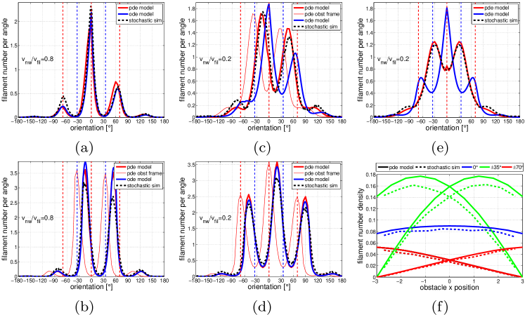
Figure 5: (a-d) Representative results for the stationary filament orientation distributions of a linear tilted obstacle obtained in the PDE-model (thick red solid line), the ODE-model (Eq. (1)) (blue solid line) and in stochastic network simulations (black dashed line). Where applicable also the transformation of the resulting PDE-model distributions to the obstacle frame is shown (thin red line). Here the orientation patterns can be interpreted as $\pm 35$ and $+70/0/\!\!-\!\!70$ patterns, that were also active in the tail of flat linear obstacles (cf. Fig. 2 & Fig. 3). The active parameters are, $\varphi=20^{\circ}$, $k_{\rm b}=20$, $d_{\rm br}^{\perp}=2\delta_{\rm fil}$ and (a) $r_{\rm br}=3$, $v_{\rm nw}/v_{\rm fil}=0.8$. (b) $r_{\rm br}=100$, $v_{\rm nw}/v_{\rm fil}=0.8$. (c) $r_{\rm br}=3$, $v_{\rm nw}/v_{\rm fil}=0.2$. (d) $r_{\rm br}=100$, $v_{\rm nw}/v_{\rm fil}=0.2$. (e) and (f) Comparison of the steady state solution for a nonperiodic linear flat obstacle from the ODE-model (Eq. (1)), the PDE-model (Eq. (47)) and stochastic network simulations. (e) For small $r_{\rm br}=3$, the ODE-solution (blue line) predicts the absence of a $\pm 35$ orientation distribution (cf. Fig. 2). However, for relatively low network velocity at $v_{\rm nw}/v_{\rm fil}=0.2$, the spatially resolved PDE-solution (red line) as well as network simulations (black dashed line) yield such a pattern. (f) The spatial filament distributions are far from uniform. Results from PDE-model (solid) and stochastic network simulation (dashed) rather show an accumulation of filaments at the lateral flanks of the obstacle, and therefore also horizontal outgrowth rates and as a direct consequence, the resulting orientation distribution averaged over the whole branching region differs from the prediction of the ODE-model.

To test our approximation, we again compared steady state filament orientation distributions, obtained by numerical iteration of Eq. (1) within the obstacle frame and subsequent transformation to the lab frame, against stochastic simulations. Typical cases are shown in Fig. 5(a)–(d) for a moderate obstacle skew angle of $\varphi=20^{\circ}$, fast and slow network velocity in the lab frame $v_{\rm nw}$, and small and large horizontal obstacle diameter as indicated by the length scale ratio $r_{\rm br}$ (Fig. 5 also shows results obtained with a PDE-model which we will introduce below). If the results are interpreted directly in the adjusted obstacle frame, very similar orientation patterns as the familiar $\pm 35$ and $+70/0/\!\!-\!\!70$ peaked distributions are realized in steady state. In the limit of very large length scale ratio $r_{\rm br}$, outgrowth in the lateral direction can be neglected again and the resulting patterns resemble orientation patterns for a network growing behind a large obstacle, only now within the rotated obstacle frame (cf. Fig. 5(b) & (d)). For small $r_{\rm br}$ in combination with a relatively high obstacle velocity, horizontal outgrowth cannot be neglected and the orientation distribution has to be interpreted in the lab frame (Fig. 5(a)). In between a transition occurs where the solutions from stochastic simulations already have to be interpreted in the obstacle frame, while results from the rate equation model are still to be interpreted directly in the lab frame (Fig. 5(c)). The reason for this is the spatial resolution in the lateral filament position, which is introduced in filament based stochastic simulations and neglected in the continuum model. Laterally nonuniform spatial filament distributions lead to differences in the effective outgrowth of filaments to the sides of the branching region. In order to include a similar spatial resolution in the continuum model, in the following we will incorporate an additional advection term in the equation. In this way it will also become possible to treat nonlinear obstacle shapes within the continuum description.

IV Nonlinear obstacle shape

In this section, we focus on actin network dynamics in the tail of curved (i.e. nonlinear) obstacle geometries. The definitions of the relevant parameters stay the same in this geometry as introduced in Fig. 1(a). Fig. 1(c) features a representative steady state network from stochastic simulation. In the following, we will stepwise extend the continuum model Eq. (1) with the goal to also incorporate nonlinear obstacle shapes in the description. We will do this first within an adjusted ordinary differential equation (ODE) model in a piecewise-linear approximation of the obstacle surface and then within a partial differential equation (PDE) model, where an advection term will explicitly govern lateral filament growth in the rate equation, additional to the reaction terms.

IV.1 Piecewise-linear obstacle approximation

Nonlinear obstacle shapes can be treated within a piecewise-linear approximation for the obstacle surface in which the ODE-model from above is still applicable. The construction of this approximation is sketched in Fig. 4(d)–(f) for a parabola-like curved obstacle surface. The branching region is divided laterally in $n$ sections of equal size $d_{{\rm br},i}^{=}=d_{\rm br}^{=}/n$ ($i=1,\dots,n$). The orthogonal width of the branching region in each section remains unchanged at $d_{{\rm br},i}^{\perp}=d_{\rm br}^{\perp}$ . The resulting obstacle approximation is a combination of lateral sections with skewed linear shape according to skew angles $\varphi_{i}$, very similar to the obstacles discussed before. The individual sections (i.e. the ODE-model equation of each section) are coupled to their direct neighbors via the lateral outgrowth rates $k_{{\rm gr},i}^{=}$ to the left and right boundaries as indicated in the sketch. In case of periodic lateral boundary conditions of the obstacle, sections $i=1$ and $i=n$ are also coupled via outgrowth. Individual outgrowth rates within the local obstacle frame of each section can then be formulated according to Eq. (44) and Eq. (45) as before.

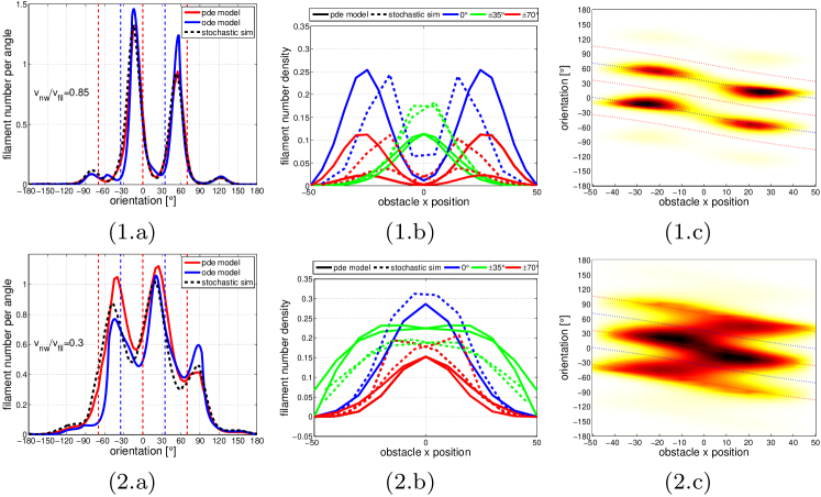
Figure 6: Typical stationary filament distributions in the tail of a nonperiodic parabolic obstacle (cf. blue solid line in Fig. 4(c)) for the parameter combinations, $\bar{\varphi}=20^{\circ}$, $r_{\rm br}=50$, $d_{\rm br}^{\perp}=2\delta_{\rm fil}$, $k_{\rm b}=20$, $k_{\rm c}=0.05$; (1) $v_{\rm nw}/v_{\rm fil}=0.85$; (2) $v_{\rm nw}/v_{\rm fil}=0.3$. (a) Filament orientation distributions spatially averaged laterally over the left hand side half space behind the symmetric obstacle. For comparison the results from PDE-model, ODE-model in triangular approximation (as illustrated by the dashed blue line in Fig. 4(c)) and stochastic simulations are shown. (b) Spatial distributions of characteristic filament angles at $\theta=0^{\circ}$, $\pm 35^{\circ}$ and $\pm 70^{\circ}$. Interpretation in the lab frame indicates coexistence of the competing $\pm 35$ and $+70/0/\!\!-\!\!70$ patterns at different lateral positions along the obstacle. (c) Heat map of the spatially resolved filament orientation distributions, where cooler colors indicate increasing filament density. Plotting dashed lines at characteristic angles at $\tilde{\theta}=0^{\circ}$, $\pm 35^{\circ}$ and $\pm 70^{\circ}$ in the obstacle frame indicates that in this frame a single familiar pattern dominates. The apparent coexistence of different patterns is artificially introduced due to a misinterpretation of the results in the lab frame.

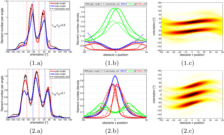
Figure 7: Same as Fig. 6 for a periodic-cosine shaped obstacle as illustrated by the solid red line in Fig. 4(c). Active parameters are $\bar{\varphi}=-20^{\circ}$, $r_{\rm br}=50$, $d_{\rm br}^{\perp}=2\delta_{\rm fil}$, $k_{\rm b}=20$, $k_{\rm c}=0.05$; (1) $v_{\rm nw}/v_{\rm fil}=0.5$; (2) $v_{\rm nw}/v_{\rm fil}=0.1$. Again an apparent coexistence of competing patterns disappears when results are interpreted in the obstacle frame, that is locally orthogonal to the obstacle surface.

Assuming a single linear obstacle is the simplest approximation of a nonlinear geometry (Fig. 4(d)). To increase accuracy, the obstacle can be subdivided laterally in ever smaller subsections. Due to the left-right symmetry of many biologically relevant obstacle shapes (e.g. the parabola-like shape in the sketch) it is sufficient to obtain results in one half-space of the obstacle geometry. This translates into a problem of $n/2$ coupled ODEs for an even number of subsections in the piecewise-linear approximation. In order to exploit this symmetry, lateral outgrowth from the section adjacent to the middle of the box has to be adjusted: Filaments that would leave the section in the middle towards the other side of the obstacle are reinjected again at this position with mirrored orientation, $\theta\rightarrow-\theta$ . For instance in case of a triangular approximation of the nonlinear obstacle (Fig. 4(e)), only the outgrowth behavior at one boundary needs adjustment compared to the problem of a skewed linear obstacle shape that was already discussed before. Fig. 6(a) and Fig. 7(a), show steady state filament orientation distributions for a laterally nonperiodic parabola and periodic-cosine shape obtained by the ODE-model in triangular approximation respectively. The nonlinear obstacle shapes together with their respective triangular approximations are illustrated in Fig. 4(c). To parametrize nonlinear parabola and cosine geometries in this context, we are using the left hand side skew angle of the triangular obstacle approximation $\bar{\varphi}$ in combination with the horizontal width of the obstacle indicated by $r_{\rm br}$.

IV.2 Reaction-advection equation

The continuum limit of an infinitely large number of piecewise-linear subsections, each of infinitesimal width, yields a PDE-model for nonlinear obstacle shapes. The model equations in this limit are complemented by an additional filament advection term, similar to hydrodynamic models, that incorporates lateral filament growth in Eq. (1),

$$\begin{split}\frac{\partial N(\theta,x,t)}{\partial t}+\frac{\partial\left(N(\theta,x,t)\cdot v_{\rm fil}^{=}(\theta,\varphi,v_{\rm nw})\right)}{\partial x}=\hat{k}_{\rm b}\int\mathcal{W}(\theta,\theta^{\prime})N(\theta^{\prime},x,t)\,\mbox{d}\theta^{\prime}\\ -k_{\rm c}N(\theta,x,t)-k_{\rm gr}^{\perp}(\theta,\varphi,v_{\rm nw})N(\theta,x,t)\,,\end{split}$$ (47)

with the horizontal filament growth speed, $v_{\rm fil}^{=}(\theta,\varphi,v_{\rm nw})$, and the vertical outgrowth rate in the lab frame, $k_{\rm gr}^{\perp}(\theta,\varphi,v_{\rm nw})$. Both, filament growth velocity and outgrowth rate are functions of filament orientation $\theta$ as well as the local obstacle skew angle $\varphi(x)$, which is active at lateral position $x$. Here again, we average outgrowth of filaments in the vertical direction by an effective rate, while horizontal growth is now spatially resolved due to the additional advection term.

For arbitrary obstacle shape, that can be expressed in terms of an analytic function $o(x)$, the local skew angle can be written as,

$$\varphi(x)=-\arctan\left(\frac{{\partial}o(x)}{{\partial}x}\right)\,.$$ (48)

The two components of the filament growth velocities within the local obstacle frame can thus be written as,

$$\tilde{v}_{\rm fil}^{\perp}(\tilde{\theta},\varphi,v_{\rm nw})=\begin{cases}0&\text{if $|\tilde{\theta}|\leq\tilde{\theta}_{\rm c}$}\\ \tilde{v}_{\rm nw}^{\perp}(\varphi)-v_{\rm fil}\cos{\tilde{\theta}}&\text{if $|\tilde{\theta}|>\tilde{\theta}_{\rm c}$}\end{cases}\,,$$ (49)

and,

$$\tilde{v}_{\rm fil}^{=}(\tilde{\theta},\varphi,v_{\rm nw})=\begin{cases}\tilde{v}_{\rm nw}^{=}(\varphi)+\tilde{v}_{\rm nw}^{\perp}(\varphi)\tan{\tilde{\theta}}&\text{if $|\tilde{\theta}|\leq\tilde{\theta}_{\rm c}$}\\ \tilde{v}_{\rm nw}^{=}(\varphi)+v_{\rm fil}\sin{\tilde{\theta}}&\text{if $|\tilde{\theta}|>\tilde{\theta}_{\rm c}$}\end{cases}\,,$$ (50)

with the components of the obstacle velocity, $\tilde{v}_{\rm nw}^{\perp}(\varphi)$ and $\tilde{v}_{\rm nw}^{=}(\varphi)$, defined as in Eq. (42) and $\tilde{\theta}_{\rm c}$ as in Eq. (46). A transformation (i.e. rotation) from the local obstacle frame into the local lab frame at each horizontal position along the obstacle surface subsequently leads to filament growth velocities, which enter the PDE-model Eq. (47) due to vertical outgrowth and advection,

$$\begin{array}[]{rccl}v_{\rm fil}^{\perp}(\theta,\varphi,v_{\rm nw})&=&&\tilde{v}_{\rm fil}^{\perp}(\tilde{\theta},\varphi,v_{\rm nw})\cos\varphi+\tilde{v}_{\rm fil}^{=}(\tilde{\theta},\varphi,v_{\rm nw})\sin\varphi\\ v_{\rm fil}^{=}(\theta,\varphi,v_{\rm nw})&=&-&\tilde{v}_{\rm fil}^{\perp}(\tilde{\theta},\varphi,v_{\rm nw})\sin\varphi+\tilde{v}_{\rm fil}^{=}(\tilde{\theta},\varphi,v_{\rm nw})\cos\varphi\,.\end{array}$$ (51)

Note, that filaments with a positive $v_{\rm fil}^{\perp}(\theta,\varphi)$ are growing vertically in opposite direction to the obstacle. Using these expressions, we can now rewrite the advection term in Eq. (47) as,

$$\frac{\partial\left(N\cdot v_{\rm fil}^{=}\right)}{\partial x}=v_{\rm fil}^{=}\frac{\partial N}{\partial x}+N\frac{\partial v_{\rm fil}^{=}}{\partial x}=v_{\rm fil}^{=}\frac{\partial N}{\partial x}+N\frac{\partial v_{\rm fil}^{=}}{\partial\varphi}\frac{\partial\varphi}{\partial x}\,,$$ (52)

with,

$$\frac{\partial v_{\rm fil}^{=}}{\partial\varphi}=-\frac{\partial\left(\tilde{v}_{\rm fil}^{\perp}\sin\varphi\right)}{\partial\varphi}+\frac{\partial\left(\tilde{v}_{\rm fil}^{=}\cos\varphi\right)}{\partial\varphi}\,,$$ (53)

and substituting Eq. (49),

$$\frac{\partial\left(\tilde{v}_{\rm fil}^{\perp}\sin\varphi\right)}{\partial\varphi}=\begin{cases}0&\text{if $|\tilde{\theta}|\leq\tilde{\theta}_{\rm c}$}\\ -v_{\rm nw}\sin^{2}\varphi+v_{\rm nw}\cos^{2}\varphi-v_{\rm fil}\cos\tilde{\theta}\cos\varphi-v_{\rm fil}\sin\varphi\sin\tilde{\theta}&\text{if $|\tilde{\theta}|>\tilde{\theta}_{\rm c}$}\end{cases}\,,$$ (54)

and Eq. (50),

$$\begin{array}[]{ll}\frac{\partial\left(\tilde{v}_{\rm fil}^{=}\cos\varphi\right)}{\partial\varphi}=&\\ \begin{cases}v_{\rm nw}\cos^{2}\varphi-v_{\rm nw}\sin^{2}\varphi-2v_{\rm nw}\cos\varphi\sin\varphi\tan\tilde{\theta}-v_{\rm nw}\cos^{2}\varphi\cos^{-2}\tilde{\theta}&\text{if $|\tilde{\theta}|\leq\tilde{\theta}_{\rm c}$}\\ v_{\rm nw}\cos^{2}\varphi-v_{\rm nw}\sin^{2}\varphi-v_{\rm fil}\sin\tilde{\theta}\sin\varphi-v_{\rm fil}\cos\varphi\cos\tilde{\theta}&\text{if $|\tilde{\theta}|>\tilde{\theta}_{\rm c}$}\end{cases}\,,\end{array}$$ (55)

and using Eq. (48),

$$\frac{\partial\varphi}{\partial x}=\frac{-\frac{{\partial^{2}}o(x)}{{\partial}x^{2}}}{1+\left(\frac{{\partial}o(x)}{{\partial}x}\right)^{2}}\,.$$ (56)

As we average outgrowth in the vertical direction by the rate $k_{\rm gr}^{\perp}(\theta,\varphi,v_{\rm nw})$ in the lab frame, while horizontal growth is now spatially resolved, we have to take into account the finite lateral movement of filaments along the obstacle geometry, when considering filaments growing out of the branching region vertically. To approximate the filament outgrowth rate accordingly, we again assume a locally linear obstacle shape at each horizontal position to find an analytical expression for the outgrowth rate in Eq. (47),

$$k_{\rm gr}^{\perp}(\theta,\varphi,v_{\rm nw})=\sqrt{\frac{{v_{\rm fil}^{\perp}}^{2}+{v_{\rm fil}^{=}}^{2}}{\left(\frac{d_{\rm br}^{\perp}/2}{v_{\rm fil}^{\perp}/v_{\rm fil}^{=}-\tan\varphi}\right)^{2}+\left(\frac{d_{\rm br}^{\perp}/2}{1-v_{\rm fil}^{=}/v_{\rm fil}^{\perp}\tan\varphi}\right)^{2}}}\,.$$ (57)

To calculate steady state filament orientation distributions from this PDE-model, Eq. (47)–Eq. (57) can be numerically iterated in discretized space and time using for instance a second order upwind scheme for the spatial differential in combination with an Euler method for temporal iteration press1992 . For this procedure, we are using a uniform filament distribution in space and orientation as initial condition and, dependent on the specific obstacle shape considered, either periodic boundary conditions or zero filament density at the respective inflow boundary.

IV.3 Linear obstacle shape revisited

The important advantage of using the PDE-model Eq. (47) compared to the initial ODE Eq. (1) to solve for steady state filament patterns clearly lies in its additional spatial resolution. This benefit not only increases the applicability of the model to a broader range of obstacle shapes, but also manifests itself when solving for specific parameter combinations for simple nonperiodic linear flat obstacles that have been already accessible using the initial ODE equations. Fig. 5(e) illustrates the steady state filament orientation distributions averaged over the whole branching region behind an obstacle of small width (i.e. $r_{\rm br}=3$). For such laterally small and flat obstacles, the ODE-model predicted the absence of the $\pm 35$ orientation pattern for arbitrary obstacle velocities $v_{\rm nw}$ (cf. Fig. 2). Due to their additional spatial resolution horizontally, the PDE-model as well as results from stochastic network simulations yield this orientation distribution nevertheless for a small range of parameters at relatively slow obstacle velocity, $v_{\rm nw}/v_{\rm fil}=0.2$. As shown in Fig. 5(f), the spatial steady state filament distributions from the PDE-model are nonuniform horizontally and in good agreement to results from stochastic simulations. This has an impact on the effective lateral outgrowth of filaments in the model and thus is able to change the final (spatially averaged) filament distributions characteristically as shown in this example.

IV.4 Parabolic and periodic-cosine obstacle shapes

The PDE-model allows us to systematically analyze actin networks in the tail of nonlinear obstacle shapes. As a proof of principle, in the following we have chosen two different obstacle shapes which are motivated by highly relevant biological examples. On the one hand, we model a laterally nonperiodic parabolic obstacle shape (blue solid line in Fig. 4(c)) which is a first approximation for the spherical or ellipsoidal shape of actin-propelled intracellular pathogens. On the other hand, actin growth behind a periodic-cosine geometry (red solid line in Fig. 4(c)) is analyzed, motivated by the laterally widely spread but corrugated leading edge of a crawling or spreading cell.

In Fig. 6 and Fig. 7, the resulting steady state patterns from the three different modeling approaches (PDE-model, ODE-model in triangular piecewise-linear approximation and stochastic network simulations) are shown for specific parameter combinations. In (a) the filament orientation distributions spatially integrated over the left side of the symmetric obstacle are shown. Here, the PDE-model corresponds very well to stochastic network simulations. Despite the rough piecewise-linear approximation of the nonlinear obstacle shape in the ODE-model, the results capture the overall characteristic of the resulting network pattern very well. Subfigures (b) illustrate the resulting spatial distributions of certain characteristic filament angles. For specific parameter cases separate spatial domains emerge over the horizontal obstacle dimension, in which the signature of the two alternative steady state network patterns, i.e. $+70/0/\!\!-\!\!70$ and $\pm 35$, are observed. For a better overview over the complete spatially resolved orientation patterns from the PDE-model, Fig. 6(c) and Fig. 7(c) illustrate the two dimensional filament distribution in heat plots, where regions of cooler color indicate higher filament density. The apparent coexistence of alternative patterns resolves when additional dotted lines are included in the heat map to indicate local filament orientations that correspond to the characteristic orientations $\tilde{\theta}=0^{\circ},\,\pm 35^{\circ},\,\pm 70^{\circ}$ within the obstacle frame, locally orthogonal to the obstacle surface along its contour. Although coexistence of alternative filament orientations is present in the lab frame, an interpretation in the local obstacle frame yields one unique pattern only that is present along the lateral extension of the obstacle.

V Discussion

In this article, we have introduced several theoretical approaches at different levels of complexity with the common goal to predict actin filament orientation patterns at the surface of stiff two dimensional obstacles, whose surfaces promote growth of actin networks. This problem is not only central for many important health and disease related biological phenomena, such as migration of animal cells or propagation of pathogens in their host, it is also a prominent example for a physical process whose properties emerge on a mesoscopic length scale in relative independence of the details of the underlying molecular processes. For example, the competition of the two fundamentally different network architectures discussed here does not rely on the exact value of the branching angle, but rather on the fact that any branching angle below 90 degrees can lead to the possibility that fundamentally different network architectures satisfy the simultaneous requirements of forward growth and side branching. Our model focuses on the geometrical aspects of this situation (in particular filament orientation and obstacle shape). In the future, it might be extended by other important aspects of this complex biological system, including the details of the filament-membrane interaction and the role of filament bending zimmermann2012 ; zhu2012 .

In general, all our results were benchmarked against stochastic computer simulations which in principle can be used to include many details of the underlying molecular processes. Here we have adopted the established view that polymerization, branching and capping are the dominating processes in the context of growing actin gels. For relatively simple linear obstacle shapes, a rate equation (ODE) model yielded accurate results and, due to its reduced complexity, also allowed for analytical progress. Using this approach, we found that either of two competing orientation patterns emerges in steady state and transitions between the two are triggered mostly by changes in the velocity of the obstacle. A similar result has already been obtained in earlier studies for a flat obstacle with large lateral extension, where filament orientation distributions with characteristic peaks at either $+70/0/\!\!-\!\!70$ or $\pm 35$ have been found to dominate the steady state of growing networks maly2001 ; weichsel2010_2 . These results were now extended to finite sized obstacles. We find that for very small objects, the $+70/0/\!\!-\!\!70$ pattern is dominant, while for larger objects, mutual stability of the two patterns recovers. In case of obstacles with a tilted straight contour (linear obstacles), again very similar patterns are predicted. However, for most parameter configurations they have to be interpreted within a rotated obstacle frame.

Curved (nonlinear) obstacle shapes have been analyzed in the ODE-model using a piecewise-linear approximation of the given geometry. As an alternative, a continuous spatial coordinate in the horizontal direction was introduced to the model equation by incorporating a filament advection term, thus yielding a PDE-model. The additional benefit of this spatial resolution clearly lies in the gain of accuracy compared to results obtained earlier. For specific parameter combinations, it was shown that the lack of spatial resolution can lead to incorrect predictions regarding the resulting filament patterns in steady state. Analysis of nonlinear obstacle shapes in the PDE-model yielded an apparent coexistence of the two competing network patterns at different horizontal positions along the obstacle surface in the lab frame. A transformation to the obstacle frame, locally at each lateral position, however revealed that one unique orientation pattern is dominating the network structure as before. Again, these results are in good agreement with computer simulations.

In order to experimentally test these theoretical predictions, the method of choice would be electron tomography urban2010 ; weichsel2012 ; vinzenz2012 , although in the future super-resolution microscopy like dual-objective STORM might become an interesting alternative xuk2012 . In the context of a rapidly increasing image quality of electron microscopy (EM) data for actin networks, the correct analysis and interpretation of the measured observables becomes increasingly important. Therefore, a detailed understanding of the structural network characteristics emerging under different situations is indispensable. In this work, we have also shown that the extracted orientation distribution of actin filament networks from experimental EM images growing at the surface of nonuniform obstacles can be easily misinterpreted. We have shown that a standard measurement in the lab frame would yield apparently novel patterns that could not be explained by existing models. For a correct interpretation of such findings, we introduced a rotated obstacle frame which lies locally orthogonal to the obstacle surface. Within this reference frame, the seemingly novel filament orientation patterns are rationalized and can be understood in terms of the two well known filament distributions, peaked at $+70/0/\!\!-\!\!70$ or $\pm 35$. Thus our results also contribute to improving the way experimental data can be compared to theoretical predictions.

A convenient setup to test our predictions would be the combination of electron tomography with biomimetic assays with particles of various shapes, which earlier have been analyzed mainly in regard to macroscopic variables such as propulsion velocity and shape of the comet tail schwartz2004 . Apart from obstacle shape, the obstacle velocity relative to the filament polymerization speed is a central parameter in the model which triggers transitions between filament orientation patterns. This velocity could be adjusted for instance by applying a force against network growth diminishing steady state growth. Changing the biochemical reaction rates for capping and branching is expected to be of minor importance and could be tested by varying the concentration of purified protein solutions in the assay. As an additional benefit of introducing different obstacle geometries in experiment, this might also lead to a deeper understanding of Arp2/3 activation close to the surface of the obstacle, which is one of the most important questions still to be clarified in the context of actin-driven motility.

- (1) M. F. Carlier, editor. Actin-based Motility. Springer Netherlands, 2010.
- (2) R. D. Mullins, J. A. Heuser, and T. D. Pollard. The interaction of Arp2/3 complex with actin: nucleation, high affinity pointed end capping, and formation of branching networks of filaments. Proceedings of the National Academy of Sciences of the United States of America, 95(11):6181–6186, 1998.
- (3) T. D. Pollard. Regulation of Actin Filament Assembly by Arp2/3 Complex and Formins. Annual Reviews in Biophysics and Biomolecular Structure, 36:451–477, 2007.
- (4) F. Frischknecht and M. Way. Surfing pathogens and the lessons learned for actin polymerization. Trends in Cell Biology, 11(1):30–38, 2001.
- (5) E. Gouin, M. D. Welch, and P. Cossart. Actin-based motility of intracellular pathogens. Current Opinion in Microbiology, 8(1):35–45, 2005.
- (6) A. Lambrechts, K. Gevaert, P. Cossart, J. Vandekerckhove, and M. Van Troys. Listeria comet tails: the actin-based motility machinery at work. Trends in Cell Biology, 18(5):220–227, 2008.
- (7) T. P. Loisel, R. Boujemaa, D. Pantaloni, and M. F. Carlier. Reconstitution of actin-based motility of Listeria and Shigella using pure proteins. Nature, 401:613–616, 1999.
- (8) L. A. Cameron, M. J. Footer, A. Van Oudenaarden, and J. A. Theriot. Motility of ActA protein-coated microspheres driven by actin polymerization. Proceedings of the National Academy of Sciences of the United States of America, 96(9):4908–4913, 1999.
- (9) A. Upadhyaya, J. R. Chabot, A. Andreeva, A. Samadani, and A. van Oudenaarden. Probing polymerization forces by using actin-propelled lipid vesicles. Proceedings of the National Academy of Sciences of the United States of America, 100(8):4521–4526, 2003.
- (10) P. A. Giardini, D. A. Fletcher, and J. A. Theriot. Compression forces generated by actin comet tails on lipid vesicles. Proceedings of the National Academy of Sciences of the United States of America, 100(11):6493–6498, 2003.
- (11) I. M. Schwartz, M. Ehrenberg, M. Bindschadler, and J. L. McGrath. The role of substrate curvature in actin-based pushing forces. Current Biology, 14(12):1094–1098, 2004.
- (12) H. Boukellal, O. Campás, J. F. Joanny, J. Prost, and C. Sykes. Soft Listeria: actin-based propulsion of liquid drops. Physical Review E, 69(6):061906, 2004.
- (13) C. C. Beltzner and T. D. Pollard. Pathway of actin filament branch formation by Arp2/3 complex. Journal of Biological Chemistry, 283(11):7135–7144, 2008.
- (14) S. Wiesner, E. Helfer, D. Didry, G. Ducouret, F. Lafuma, M. F. Carlier, and D. Pantaloni. A biomimetic motility assay provides insight into the mechanism of actin-based motility. Journal of Cell Biology, 160(3):387–398, 2003.
- (15) J. L. McGrath, N. J. Eungdamrong, C. I. Fisher, F. Peng, L. Mahadevan, T. J. Mitchison, and S. C. Kuo. The force-velocity relationship for the actin-based motility of Listeria monocytogenes. Current Biology, 13(4):329–332, 2003.
- (16) Y. Marcy, J. Prost, M. F. Carlier, and C. Sykes. Forces generated during actin-based propulsion: a direct measurement by micromanipulation. Proceedings of the National Academy of Sciences of the United States of America, 101(16):5992–5997, 2004.
- (17) S. H. Parekh, O. Chaudhuri, J. A. Theriot, and D. A. Fletcher. Loading history determines the velocity of actin-network growth. Nature Cell Biology, 7(12):1219–1223, 2005.
- (18) M. Prass, K. Jacobson, A. Mogilner, and M. Radmacher. Direct measurement of the lamellipodial protrusive force in a migrating cell. Journal of Cell Biology, 174(6):767–772, 2006.
- (19) F. Heinemann, H. Doschke, and M. Radmacher. Keratocyte lamellipodial protrusion is characterized by a concave force-velocity relation. Biophysical Journal, 100(6):1420–1427, 2011.
- (20) J. Zimmermann, C. Brunner, M. Enculescu, M. Goegler, A. Ehrlicher, J. Käs, and M. Falcke. Actin Filament Elasticity and Retrograde Flow Shape the Force-Velocity Relation of Motile Cells. Biophysical Journal, 102(2):287–295, 2012.
- (21) G. P. Resch, E. Urban, and S. Jacob. The actin cytoskeleton in whole mount preparations and sections. Methods in Cell Biology, 96:529–564, 2010.
- (22) M. Vinzenz, M. Nemethova, F. Schur, J. Mueller, A. Narita, E. Urban, C. Winkler, C. Schmeiser, S.A. Koestler, K. Rottner, et al. Actin branching in the initiation and maintenance of lamellipodia. Journal of Cell Science, 125(11):2775–2785, 2012.
- (23) T. M. Svitkina and G. G. Borisy. Arp2/3 Complex and Actin Depolymerizing Factor/Cofilin in Dendritic Organization and Treadmilling of Actin Filament Array in Lamellipodia. The Journal of Cell Biology, 145(5):1009–1026, 1999.
- (24) E. Urban, S. Jacob, M. Nemethova, G. P. Resch, and J. V. Small. Electron tomography reveals unbranched networks of actin filaments in lamellipodia. Nature Cell Biology, 12(5):429–435, 2010.
- (25) S. A. Koestler, S. Auinger, M. Vinzenz, K. Rottner, and J. V. Small. Differentially oriented populations of actin filaments generated in lamellipodia collaborate in pushing and pausing at the cell front. Nature Cell Biology, 10(3):306–313, 2008.
- (26) J. Weichsel, E. Urban, J. V. Small, and U. S. Schwarz. Reconstructing the orientation distribution of actin filaments in the lamellipodium of migrating keratocytes from electron microscopy tomography data. Cytometry Part A, 81A(6):496–507, 2012.
- (27) A. E. Carlsson and A. Mogilner. Mathematical and physical modeling of actin dynamics in motile cells. Actin-based Motility, M. F. Carlier (Ed.), Springer 2010.
- (28) A. Mogilner and G. Oster. Cell motility driven by actin polymerization. Biophysical Journal, 71(6):3030–3045, 1996.
- (29) A. Mogilner and G. Oster. Force generation by actin polymerization II: the elastic ratchet and tethered filaments. Biophysical Journal, 84(3):1591–1605, 2003.
- (30) A. E. Carlsson. Growth velocities of branched actin networks. Biophysical Journal, 84(5):2907–2918, 2003.
- (31) I. V. Maly and G. G. Borisy. Self-organization of a propulsive actin network as an evolutionary process. Proceedings of the National Academy of Sciences of the United States of America, 98(20):11324–11329, 2001.
- (32) J. Weichsel and U. S. Schwarz. Two competing orientation patterns explain experimentally observed anomalies in growing actin networks. Proceedings of the National Academy of Sciences of the United States of America, 107(14):6304–6309, 2010.
- (33) T. E. Schaus and G. G. Borisy. Performance of a population of independent filaments in lamellipodial protrusion. Biophysical Journal, 95(3):1393–1411, 2008.
- (34) K. C. Lee and A. J. Liu. Force-Velocity Relation for Actin-Polymerization-Driven Motility from Brownian Dynamics Simulations. Biophysical Journal, 97(5):1295–1304, 2009.
- (35) J. B. Alberts and G. M. Odell. In silico reconstitution of Listeria propulsion exhibits nano-saltation. PLoS biology, 2(12):e412, 2004.
- (36) C. H. Schreiber, M. Stewart, and T. Duke. Simulation of cell motility that reproduces the force–velocity relationship. Proceedings of the National Academy of Sciences of the United States of America, 107(20):9141–9146, 2010.
- (37) F. Gerbal, P. Chaikin, Y. Rabin, and J. Prost. An elastic analysis of listeria monocytogenes propulsion. Biophysical journal, 79(5):2259–2275, 2000.
- (38) J. Zhu and A. Mogilner. Mesoscopic Model of Actin-Based Propulsion. PLoS Computational Biology, 8(11):e1002764, 2012.
- (39) A. B. Verkhovsky, O. Y. Chaga, S. Schaub, T. M. Svitkina, J. J. Meister, and G. G. Borisy. Orientational Order of the Lamellipodial Actin Network as Demonstrated in Living Motile Cells. Molecular Biology of the Cell, 14(11):4667–4675, 2003.
- (40) S. Schaub, J. J. Meister, and A. B. Verkhovsky. Analysis of actin filament network organization in lamellipodia by comparing experimental and simulated images. Journal of Cell Science, 120(8):1491–1500, 2007.
- (41) C. A. Ydenberg, B. A. Smith, D. Breitsprecher, J. Gelles, and B. L. Goode. Cease-fire at the leading edge: New perspectives on actin filament branching, debranching, and cross-linking. Cytoskeleton, 68(11):596–602, 2011.
- (42) S.-C. Ti, C. T. Jurgenson, B. J. Nolen, and T. D. Pollard. Structural and biochemical characterization of two binding sites for nucleation-promoting factor wasp-vca on arp2/3 complex. Proceedings of the National Academy of Sciences of the United States of America, 108(33):E463–E471, 2011.
- (43) X. P. Xu, I. Rouiller, B. D. Slaughter, C. Egile, E. Kim, J. R. Unruh, X. Fan, T. D. Pollard, R. Li, D. Hanein, and N. Volkmann. Three-dimensional reconstructions of Arp2/3 complex with bound nucleation promoting factors. The EMBO Journal, 31(1):236–247, 2012.
- (44) D.A. Schafer, P.B. Jennings, and J.A. Cooper. Dynamics of capping protein and actin assembly in vitro: uncapping barbed ends by polyphosphoinositides. The Journal of Cell Biology, 135(1):169–179, 1996.
- (45) J. Käs, H. Strey, and E. Sackmann. Direct imaging of reptation for semiflexible actin filaments. Nature, 368(6468):226–229, 1994.
- (46) M. A. Dichtl and E. Sackmann. Colloidal probe study of short time local and long time reptational motion of semiflexible macromolecules in entangled networks. New Journal of Physics, 1(1):18, 1999.
- (47) T. D. Pollard, L. Blanchoin, and R. D. Mullins. Molecular mechanism controlling actin filament dynamics in nonmuscle cells. Annual Reviews in Biophysics and Biomolecular Structure, 29(1):545–576, 2000.
- (48) J. Weichsel and U. S. Schwarz. Unifying autocatalytic and zeroth order branching models for growing actin networks. Arxiv preprint arXiv:1207.4574, 2012.
- (49) W. H. Press, S. A. Teukolsky, W. T. Vetterling, and B. P. Flannery. Numerical recipes in C: the art of scientific computing. Cambridge University Press, 1992.
- (50) K. Xu, H. P. Babcock, and X. Zhuang. Dual-objective STORM reveals three-dimensional filament organization in the actin cytoskeleton. Nature Methods, 9(2):185–188, 2012.