Numerical simulation of red blood cell suspensions behind a moving interface in a capillary Shihai Zhao and Tsorng-Whay Pan Department of Mathematics, University of Houston, Houston, Texas 77204-3008, USA

Abstract: Computational modeling and simulation are presented on the motion of red blood cells behind a moving interface in a capillary. The methodology is based on an immersed boundary method and the skeleton structure of the red blood cell (RBC) membrane is modeled as a spring network. The computational domain is moving with either a designated RBC or an interface in an infinitely long two-dimensional channel with an undisturbed flow field in front of the domain. The tanking-treading and the inclination angle of a cell in a simple shear flow are briefly discussed for the validation purpose. We then present the results of the motion of red blood cells behind a moving interface in a capillary, which show that the RBCs with higher velocity than the interface speed form a concentrated slug behind the interface.

Key words: red blood cells, moving domain, immersed boundary method.

1 Introduction

The rheological property of the red blood cells (RBCs) is a key factor of the blood flow characteristics at the microchannel level, especially the particulate nature of the blood becomes significant when studying blood drop through a glass capillary within miniature blood diagnostic kit. The penetration of the blood suspension in a perfectly wettable capillary has been analyzed in [1, 2]. The failure of such penetration is attributed to three RBCs segregation mechanisms: (i) corner deflection at the entrance, (ii) the intermediate deformation-induced radial migration and (iii) shear-induced diffusion within a packed slug at the meniscus. The key mechanism responsible for penetration failure is the deformation-induced radial migration, which endows the blood cells with a higher velocity than the meniscus to form the concentrated slug behind the meniscus (see Figure 1). The results in [1, 2] shed light on making the smallest microfluidic kit and loading microneedle that require the least amount of blood sample.

Nowadays in silico mathematical modeling and numerical study of RBC rheology have attracted growing interest (see, e.g., [3, 4]). The immersed boundary method developed by Peskin, e.g, [5, 7, 6], has been one of the popular methodologies for numerically studying the RBC rheology due its distinguish features in dealing with the problem of fluid flow interacting with a flexible fluid/structure interface. For example, in [8]-[17], immersed boundary methods have been combined with different RBC membrane models to simulate the motion of RBCs and vesicles in fluid flow. In [15, 16, 17], we have successfully combined an immersed boundary method with a spring model developed in [18] to simulate the motion of RBCs in shear flows and Poiseuille flows. In this paper we have generalized the aforementioned methodology to simulate the RBCs aggregation behind a moving interface considered in [1, 2] by having the computational domain moving with an interface in an infinitely long two-dimensional channel with an undisturbed flow field in front of the domain since the typical periodic boundary condition in the direction of the channel wall is not well suited anymore. To mimic the motion of the RBCs behind a meniscus in a capillary, we have considered a flat interface moving with a given constant speed in this paper. The simulating results of the motion of red blood cells behind a moving interface show that the RBCs with higher velocity than the interface speed form the concentrated slug behind the interface, which resembles the motion of the RBCs observed in [1, 2]. The structure of this paper is as follows: We discuss the elastic spring model and numerical methods in Section 2. In Section 3, the tanking-treading and the inclination angle of a cell in a simple shear flow are briefly discussed for the validation purpose. We then present the results of the motion of red blood cells behind a moving interface in a capillary. The conclusions are summarized in Section 4.

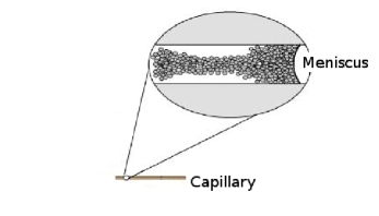
Figure 1: Schematics of the BRCs moving behind a meniscus.

2 Models and methods

Let $\Omega$ be a bounded rectangular domain filled with blood plasma which is incompressible, Newtonian, and contains RBCs with the viscosity of the cytoplasm same as that of the blood plasma (see Figure 2). For some $T>0$, the governing equations for the fluid-cell system are

$$\rho\displaystyle\left[\frac{\partial{\bf u}}{\partial t}+{\bf u}\cdot{\boldsymbol{\nabla}}{\bf u}\right]=-{\boldsymbol{\nabla}}p+\mu\Delta{\bf u}+{\bf f}\ \text{in}\enspace\Omega,\ t\in(0,T),$$ (2.1)

$${\boldsymbol{\nabla}}\cdot{\bf u}=0\enspace\text{in}\enspace\Omega,\enspace t\in(0,T)$$ (2.2)

where ${\bf u}$ and $p$ are the fluid velocity and pressure, respectively, $\rho$ is the fluid density, and $\mu$ is the fluid viscosity, which is assumed to be constant for the entire computational domain. In (2.1), ${\bf f}$ is a body force which accounts for the force acting on the fluid/cell interface. Equations (2.1) and (2.2) are completed by the following boundary and initial conditions:

$${\bf u}={\bf g}_{0}\enspace\text{on}\enspace\Gamma_{d},$$ (2.3)

$$\mu\dfrac{{\partial\bf u}}{\partial\bf n}-{\bf n}p={\bf 0}\enspace\text{on}\enspace\Gamma_{n},$$ (2.4)

$${\bf u}(0)={\bf u}_{0}$$ (2.5)

where the domain $\Omega$ is taken from an infinitely long channel with its boundary denoted by $\displaystyle\Gamma=\cup_{i=1}^{4}\Gamma_{i}$. In the simulations, we have considered two types of boundary conditions: (i) $\Gamma_{n}=\emptyset$ and $\Gamma_{d}=\Gamma$, (ii) $\Gamma_{n}=\Gamma_{4}$ and $\Gamma_{d}=\Gamma_{1}\cup\Gamma_{2}\cup\Gamma_{3}$ with ${\bf g}_{0}$ having the profile of either Poiseuille flow or simple shear flow on $\Gamma_{d}$

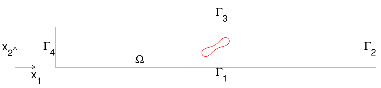
Figure 2: An example of the computational domain with a cell.

2.1 Elastic spring model for the RBC membrane

A two-dimensional elastic spring model used in [18] is considered in this paper to describe the deformable behavior of the RBCs. Based on this model, the RBC membrane can be viewed as membrane particles connecting with the neighboring membrane particles by springs, as shown in Figure 3. Elastic energy stores in the spring due to the change of the length $l$ of the spring with respected to its reference length $l_{0}$ and the change in angle $\theta$ between two neighboring springs. The total elastic energy of the RBC membrane, $E=E_{l}+E_{b}$, is the sum of the total elastic energy for stretch/compression and the total energy for bending which, in particular, are

$$E_{l}=\frac{k_{l}}{2}\sum_{i=1}^{N}(\frac{l_{i}-l_{0}}{l_{0}})^{2}$$ (2.6)

and

$$E_{b}=\frac{k_{b}}{2}\sum_{i=1}^{N}tan^{2}(\theta_{i}/2).$$ (2.7)

Figure 3: The elastic spring model of the RBC membrane

In equations (2.6) and (2.7), $N$ is the total number of the spring elements, and $k_{l}$ and $k_{b}$ are spring constants for changes in length and bending angle, respectively.

Remark 2.1.

In the process of creating the initial shape of RBCs described in [18], the RBC is assumed to be a circle of radius $R_{0}=2.8\ \mu m$ initially. The circle is discretized into $N=76$ membrane particles so that $76$ springs are formed by connecting the neighboring particles. The shape change is stimulated by reducing the total area of the circle through a penalty function

$$\Gamma_{s}=\frac{k_{s}}{2}(\frac{s-s_{e}}{s_{e}})^{2}$$ (2.8)

where $s$ and $s_{e}$ are the time dependent area of the RBC and the equilibrium area of the RBC, respectively, and the total energy is modified as $E+\Gamma_{s}$. Based on the principle of virtual work the force acting on the $i$th membrane particle now is

$${\bf F}_{i}=-\frac{\partial(E+\Gamma_{s})}{\partial{\bf r}_{i}}$$ (2.9)

where ${\bf r}_{i}$ is the position of the $i$th membrane particle. When the area is reduced, each RBC membrane particle moves on the basis of the following equation of motion:

$$m\ddot{{\bf r}_{i}}+\gamma\dot{{\bf r}_{i}}={\bf F}_{i}$$ (2.10)

Here, $\dot{()}$ denotes the time derivative; $m$ and $\gamma$ represent the membrane particle mass and the membrane viscosity of the RBC. The position ${\bf r}_{i}$ of the $i$th membrane particle is solved by discretizing (2.10) via a second order finite difference method. The total energy stored in the membrane decreases as the time elapses. The final shape of the RBC is obtained as the total elastic energy is minimized (please see [19]). The area of the final shape has less than $0.001\%$ difference from the given equilibrium area $s_{e}$ and the length of the perimeter of the final shape has less than $0.005\%$ difference from the circumference of the initial circle. The reduced area of a RBC in this paper is defined by $s^{*}=s_{e}/\pi R_{0}^{2}$.

Remark 2.2.

When simulating the case involving a moving interface, we have applied a repulsive force to prevent the overlapping between cell and wall. The repulsive force is obtained from the following Morse potential (e.g., see [20])

$$\phi(d)=k_{r}(1-e^{-(d-d_{0})})^{2}$$

where the parameter $d$ is the shortest distance between the membrane particle and the wall and $d_{0}$ is the range of the repulsive force (when the distance $d$ is greater than $d_{0}$, there is no repulsive force). The parameter $k_{r}$ is a constant for the strength of the potential.

2.2 Immersed boundary method

The immersed boundary method developed by Peskin, e.g, [5, 7, 6], is employed in this study because of its distinguish features in dealing with the problem of fluid flow interacting with a flexible fluid/structure interface. Over the years, it has demonstrated its capability in study of computational fluid dynamics including blood flow. Based on the method, the boundary of the deformable structure is discretized spatially into a set of boundary nodes. The force located at the immersed boundary node ${\bf r}_{i}=(r_{i,1},r_{i,2})$ affects the nearby fluid mesh nodes ${\bf x}=(x_{1},x_{2})$ through a 2D discrete $\delta$-function $D_{h}({\bf x}-{\bf r}_{i})$:

$${\bf f}({\bf x})=\sum{\bf F}_{i}D_{h}({\bf x}-{\bf r}_{i})\ \ for\ \lvert{\bf x}-{\bf r}_{i}\rvert\leq 2h,$$ (2.11)

where $h$ is the uniform finite element mesh size and

$$D_{h}({\bf x}-{\bf r}_{i})=\delta_{h}(x_{1}-r_{i,1})\delta_{h}(x_{2}-r_{i,2})$$ (2.12)

with the 1D discrete $\delta$-functions being

$$\delta_{h}(z)=\begin{cases}\frac{1}{8h}\left(3-{2|z|}/{h}+\sqrt{1+{4|z|}/{h}-4({|z|}/{h})^{2}}\right),&\ \lvert z\rvert\leq h,\\ \frac{1}{8h}\left(5-{2|z|}/{h}-\sqrt{-7+{12|z|}/{h}-4({|z|}/{h})^{2}}\right),&\ h\leq\ \lvert z\rvert\leq 2h,\\ 0,&\ otherwise.\end{cases}$$ (2.13)

The velocity of the immersed boundary node ${\bf r}_{i}$ is also affected by the surrounding fluid and therefore is enforced by summing the velocities at the nearby fluid mesh nodes ${\bf x}$ weighted by the same discrete $\delta$-function:

$${\bf U}({\bf r}_{i})=\sum h^{2}{\bf u(x)}D_{h}({\bf x}-{\bf r}_{i})\ \ for\ \lvert{\bf x}-{\bf x}_{i}\rvert\leq 2h.$$ (2.14)

After each time step, the position of the immersed boundary node is updated by

$${\bf r}_{i}^{n+1}={\bf r}_{i}^{n}+\Delta{t}{\bf U}({\bf r}_{i}^{n}).$$ (2.15)

2.3 Space approximation and time discretization

Concerning the finite element based space approximation of $\{{\bf u},p\}$ in problem (2.1)-(2.5), we use the $P_{1}$-$iso$-$P_{2}$ and $P_{1}$ finite element approximation (e.g., see [22] (Chapter 5)). For a rectangular computational domain $\Omega\subset R^{2}$, let ${\mathcal{T}}_{h}$ be a finite element triangulation of $\overline{\Omega}$ for velocity and ${\mathcal{T}}_{2h}$ a twice coarser triangulation for pressure where $h$ is a space discretization step. We introduce the finite dimensional spaces:

$$W_{h}=\{{\bf v}_{h}|{\bf v}_{h}\in C^{0}(\overline{\Omega})^{2},{\bf v}_{h}|_{T}\in P_{1}\times P_{1},\forall T\in{\mathcal{T}}_{h}\}$$

$$W_{0h}=\{{\bf v}_{h}|{\bf v}_{h}\in W_{h},{\bf v}_{h}={\bf 0}\ \text{on}\ \Gamma_{d}\},$$

$$L_{h}^{2}=\{q_{h}|q_{h}\in C^{0}(\overline{\Omega}),q_{h}|_{T}\in P_{1},\forall T\in{\mathcal{T}}_{2h}\ \},$$

$$L_{h,0}^{2}=\{q_{h}|q_{h}\in L_{h}^{2},\int_{\Omega}q_{h}\,d{\bf x}=0\}$$

where $P_{1}$ is the space of polynomials in two variables of degree $\leq 1$. We apply the Lie’s scheme [21, 22] with the above finite elements to equations (2.1)-(2.5) with the backward Euler method in time for some subproblems and obtain the following sequence of fractional step subproblems (some of the subscripts $h$ have been dropped):

${\bf u}^{0}={\bf u}_{0}$ is given; for $n\geq 0$, ${\bf u}^{n}$ being known, we compute the approximate solution via the following fractional steps:

1. Update the position of the membrane by (2.14) and (2.15) and then compute the force ${\bf f}^{n}$ based on the fluid/cell interface by (2.9) and (2.11).

2. Solve

   $$\left\{\begin{array}[]{ll}\displaystyle\int_{\Omega}\frac{\partial{\bf u}(t)}{\partial t}\cdot{\bf v}d{\bf x}+\int_{\Omega}({\bf u}^{n}\cdot{\boldsymbol{\nabla}}){\bf u}(t)\cdot{\bf v}d{\bf x}=0,\ \enspace\text{on}\,\enspace(t^{n},t^{n+1}),\enspace\forall{\bf v}\in W_{0h}^{-},\\ {\bf u}(t^{n})={\bf u}^{n},\\ {\bf u}(t)\in W_{h},\ {\bf u}(t)={\bf g}_{0,h}\ \enspace\text{on}\,\enspace\Gamma^{-}\times(t^{n},t^{n+1}),\end{array}\right.\\$$ (2.16)

   and set ${\bf u}^{n+2/3}={\bf u}(t^{n+1})$.

3. Finally solve

   $$\ \left\{\begin{array}[]{ll}\displaystyle\rho\int_{\Omega}\frac{{\bf u}^{n+1}-{\bf u}^{n+2/3}}{\triangle t}\cdot{\bf v}d{\bf x}+\mu\int_{\Omega}{\boldsymbol{\nabla}}{\bf u}^{n+1}\boldsymbol{:}{\boldsymbol{\nabla}}{\bf v}d{\bf x}\\ \hskip 20.0pt-\displaystyle\int_{\Omega}p^{n+1}({\boldsymbol{\nabla}}\cdot{\bf v})d{\bf x}\displaystyle=\int_{\Omega}{\bf f}^{n}\cdot{\bf v}d{\bf x},\enspace\forall{\bf v}\in W_{0h},\\ \displaystyle\int_{\Omega}q{\boldsymbol{\nabla}}\cdot{\bf u}^{n+1}d{\bf x}=0,\enspace\forall q\in L_{h}^{2},\\ {\bf u}^{n+1}\in W_{h},\ {\bf u}(t)={\bf g}_{0,h}\ \text{on}\ \Gamma_{d};\ p^{n+1}\in L_{h}^{2}\ (p^{n+1}\in L_{h,0}^{2}\ \text{if}\ \Gamma_{n}=\emptyset).\end{array}\right.$$ (2.17)

In eq. (2.16), we have $\Gamma^{-}=\{{\bf x}|{\bf x}\in\Gamma$, ${\bf g}_{0,h}({\bf x})\cdot{\bf n}({\bf x})<0$ $\}$ and $W_{0h}^{-}=\{{\bf v}_{h}|{\bf v}_{h}\in W_{h},{\bf v}_{h}={\bf 0}\ \text{on}\ \Gamma^{-}\}$. The quasi-Stokes problem (2.17) is solved by a preconditioned conjugate gradient method (see, e.g., [22]). The subproblem (2.16) is an advection type subproblem. It is solved by a wave-like equation method, which is described in detail in [23] and [24].

Remark 2.3.

In simulations, the computational domain $\Omega$ moves to the right with either the mass center of a RBC or the interface (see, e.g., [25, 26] and references therein for adjusting the computational domain according to the position of the particle). Due to the use of structured and uniform mesh in our simulations, it is relatively easy to have the computational domain moving with a designated cell. Generally when the mass center of a RBC moves to the right in an infinitely long channel, we add one vertical grid line to the right end of the computational domain if the cell mass center crosses one vertical grid line after we predict its new position and at the same time we drop one vertical grid line at the left end of the computational domain. In the mean time at these new grid points added at the right end, we assign the values of velocity field according to either Poiseuille flow or simple shear flow depending on the test cases. When following an interface moving to the right with a constant speed, we have applied the same strategy.

3 Numerical results and discussion

3.1 Tank-treading of a single cell in shear flow

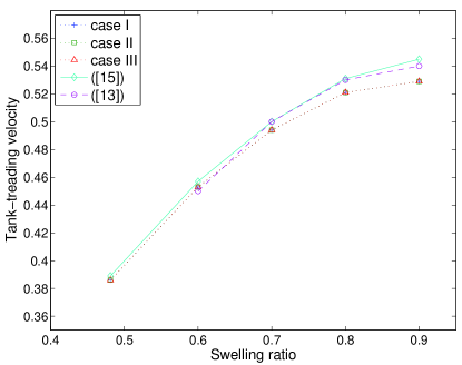
Figure 4: (Color online). Steady inclination angle versus the cell swelling ratio (left) and membrane tank-treading velocity (scaled by $\gamma R_{0}/2$) versus the cell swelling ratio (right) in comparison to Shi. et al.[15] and Kaoui. et al.[13] in different cases. Case I: $112\rm{\mu m}\times 7\rm{\mu m}$ domain with Dirichlet boundary conditions, Case II: $80\rm{\mu m}\times 7\rm{\mu m}$ domain with Dirichlet boundary conditions, Case III: $80\rm{\mu m}\times 7\rm{\mu m}$ domain with Neumann inflow condition and Dirichlet outflow condition.

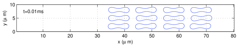
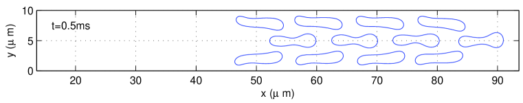
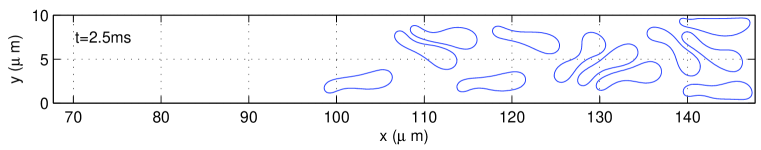
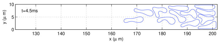
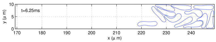
Figure 5: (Color online). The positions of 12 cells in a capillary behind a moving interface at $t=$ 0.01, 0.5, 2.5, 4.5 and 6.25 ms and the velocity field with 12 cells at $t=$6.25 ms (from top to bottom).

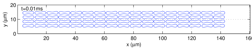
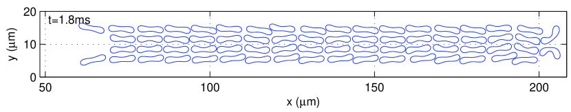
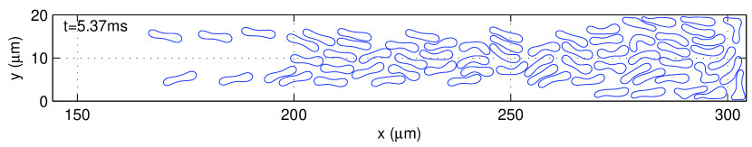
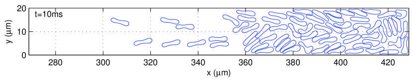
Figure 6: (Color online). The position of 68 cells in a capillary behind a moving interface at $t=$ 0.01, 1.8, 5.37 and 10 ms and the velocity field with 68 cells at $t=$ 5.37 and 10 ms (from top to bottom).

We have first validated the computational methodology with two types of boundary conditions discussed in Section 2 by comparing the inclination angle and the tank-treading frequency of a single RBC in shear flow. Here are the parameters used in the simulations: The values of parameters for modeling cells are same with [15, 16, 17] as follows: The bending constant is $k_{b}=5\times 10^{-10}\rm{N\cdot m}$, the spring constant is $k_{l}=5\times 10^{-8}\rm{N\cdot m}$, the penalty coefficient is $k_{s}=10^{-5}\rm{N\cdot m}$, the repulsive force coefficient is $k_{r}=10^{-9}\rm{N\cdot m}$, and the range of the repulsive force is $d_{0}=2h$ where $h$ is the mesh size for the flow velocity field. The cells are suspended in blood plasma which has a density $\rho=1.00\rm{g/cm^{3}}$ and a dynamical viscosity $\mu=0.012\rm{g/(cm\cdot s)}$. The viscosity ratio which describes the viscosity contrast of the inner and outer fluid of the RBC membrane is fixed at 1.0. The dimensions of the computational domain are $112\rm{\mu m}\times 7\rm{\mu m}$ and $80\rm{\mu m}\times 7\rm{\mu m}$. Then the degree of confinement ($2R_{0}/H$) is 0.8 where $H$ is the height of the channel. The grid resolution for the computational domain is 80 grid points per 10$\rm{\mu m}$. The time step $\Delta t$ is $1\times 10^{-5}\rm{ms}$. The initial position of the mass center of the cells are (56, 3.5) and (40, 3.5) for the longer domain and the shorter domain, respectively. To have a shear flow, a Couette flow driven by two walls at the top and bottom which have the same speed $U/2$ but move in directions opposite to each other is applied to the suspension, where the speed $U$ is given by $U=\gamma*H$ with a given shear rate $\gamma$. The shear rate used in the simulation is $\gamma=275$/s. The steady inclination angles of the tank-treading for four values of $s^{*}$=0.6, 0.7, 0.8 and 0.9 are presented in Figure 4, which show the very good agreement with the lattice-Boltzmann simulation results in [13] and those previously obtained with periodic boundary conditions in [15]. The membrane tank-treading velocity (scaled by $\gamma R_{0}/2$) is also in good agreement with the results in [13, 15]. The results show that there is no significant difference when having the Dirichlet boundary conditions on $\Gamma$ with the length $L=112$ and $80\ \rm{\mu m}$ or the conditions (2.3) and (2.4) on the boundary of the shorter domain.

3.2 Multi-cell aggregation in a capillary behind a moving interface

For the cases involving a moving interface in a capillary, we have considered the one moving to the right with constant speed $U$ to mimic the motion of the RBCs behind a meniscus in a capillary. Then the associated boundary condition in (2.3) on $\Gamma_{d}$ is ${\bf g}_{0}={\bf 0}$ on $\Gamma_{1}\cup\Gamma_{3}$ and ${\bf g}_{0}=(U,0)^{t}$ on $\Gamma_{2}$ and the boundary condition (2.4) is satisfied on $\Gamma_{4}$. We have kept all the related parameters the same except the following. We have first considered the case of 12 cells of swelling ratio $s^{*}$=0.481 in a capillary of the height $10\rm{\mu m}$. The computational domain $\Omega$ is $80\rm{\mu m}\times 10\rm{\mu m}$. The interface speed is $U=8/3$ cm/s. The cells in the center of the channel move faster than those next to the top and bottom walls do due to fact that the velocity field behaves like Poiseuille flow as the fluid flow is away from the interface and the speed of the interface is slower than the velocity of the fluid flow in the channel central region away from the interface (see the velocity field in Figures 5 and 6). For the cells moving away from the interface, they move back to the central region of the channel due to the lateral migration of the cells in a flow field like the Poiseuille flow and then move toward the interface. Thus the cells form a slug behind the moving interface and move with the interface as in Figure 5. For the case of 68 cells of swelling ratio $s^{*}$=0.481 in a capillary of the height $20\rm{\mu m}$, we have considered the computational domain $\Omega=160\rm{\mu m}\times 20\rm{\mu m}$. The interface speed is $U=8/3$ cm/s. These 68 cells behave similarly behind the moving interface like the motion of the 12 cells considered in the previous case. But it is much clearly for us to see that the cells in the channel central region move faster to the right due to the relatively faster flow field. Then the cells are piled up behind the interface and move with the interface in Figure 6.

4 Conclusions

In summary, we have developed computational modeling and methodologies for simulating the motion of many RBCs in a capillary behind a moving interface in this paper. The methodology is based on an immersed boundary method and the skeleton structure of the red blood cell (RBC) membrane is modeled as a spring network. The computational domain is moving with either a designated RBC or an interface in an infinitely long two-dimensional channel with an undisturbed flow field in front of the domain. The tanking-treading and the inclination angle of a cell in a simple shear flow are briefly discussed for the validation purpose. The results of the motion of red blood cells behind a moving interface in a capillary show that the RBCs with higher velocity than the interface speed form a concentrated slug behind the interface, which is consistent with the results in [1, 2]. The lateral migration is also a key factor for the formation of a slug behind the moving interface.

References

- [1] H.-C. Chang, R. Zhou, Capillary penetration failure of blood suspensions, J. Colloid Interface Sci. 287 (2005), pp. 647–656.
- [2] R. Zhou, J. Gordon, A.F. Palmer, H.-C. Chang, Role of erythrocyte deformability during capillary wetting, Biotechnology and Bioengineering 93 (2006), pp. 201-–211.
- [3] V. Cristini, G.S. Kassab, Computer odeling of red blood cell rheology in the microcirculation: a brief overview., Ann. Biomed. Eng. 33 (2005), pp. 1724–1727.
- [4] C. Pozrikidis, Modeling and simulation of capsules and biological cells. Chapman & Hall/CRC: Boca Raton, 2003.
- [5] C.S. Peskin, Numerical analysis of blood flow in the heart, J. Comput. Phys., 25 (1977), pp. 220–252.
- [6] C.S. Peskin, The immersed boundary method, Acta Numer., 11 (2002), pp. 479–517.
- [7] C.S. Peskin, D.M. McQueen, Modeling prosthetic heart valves for numerical analysis of blood flow in the heart, J. Comput. Phys., 37 (1980), pp. 113-–32.
- [8] C. Eggleton, A. Popel, Large deformation of red blood cell ghosts in a simple shear flow, Phys. Fluids, 10 (1998), pp. 1834–1845.
- [9] P. Bagchi, P. Johnson, A. Popel, Computational Fluid Dynamic Simulation of Aggregation of Deformable Cells in a Shear Flow, J. Biomech. Eng., 127 (2005), pp. 1070–1080.
- [10] P. Bagchi, Mesoscale simulation of blood flow in small vessels, Biophys. J., 92 (2007), pp. 1858–1877.
- [11] J. Zhang, J. Johnson, A.S. Popel, Effects of erythrocyte deformability and aggregation on the cell free layer and apparent viscosity of microscopic blood flows, Microvasc. Res., 77 (2009), pp. 265–272.
- [12] L.M. Crowl, A.L. Fogelson, Computational model of whole blood exhibiting lateral platelet motion induced by red blood cells, Int. J. Numer. Meth. Biomed. Engng., 26 (2010), pp. 471–487.
- [13] B. Kaoui, J. Harting, C. Misbah, Two-dimensional vesicle dynamics under shear flow: Effect of confinement, Phys. Rev. E, 83 (2011), 066319.
- [14] Y. Kim, M.-C. Lai, Numerical study of viscosity and inertial effects on tank-treading and tumbling motions of vesicles under shear flow, Phys. Rev. E, 86 (2012), 066321.
- [15] L. Shi, T.-W. Pan, R. Glowinski, Deformation of a single blood cell in bounded Poiseuille flows, Phys. Rev. E, 85 (2012), 016307.
- [16] L. Shi, T.-W. Pan, R. Glowinski, Lateral migration and equilibrium shape and position of a single red blood cell in bounded Poiseuille flows, Phys. Rev. E, 86 (2012), 056308.
- [17] L. Shi, T.-W. Pan, R. Glowinski, Numerical simulation of lateral migration of red blood cells in Poiseuille flows, Int. J. Numer. Methods Fluids, 68 (2012), pp. 1393–1408.
- [18] K. Tsubota, S. Wada, T. Yamaguchi, Simulation study on effects of hematocrit on blood flow properties using particle method, J. Biomech. Sci. Eng., 1 (2006), pp. 159–170.
- [19] T. Wang, T.-W. Pan, Z. Xing, R. Glowinski, Numerical simulation of rheology of red blood cell rouleaux in microchannels, Phys. Rev. E, 79 (2009), 041916.
- [20] A. Alexeev, R. Verberg, A.C. Balazs, Modeling the interactions between deformable capsules rolling on a compliant surface, Soft Matter 2 (2006), pp. 499–509.
- [21] A.J. Chorin, T.J.R. Hughes, M.F. McCracken, J.E. Marsden, Product formulas and numerical algorithms, Comm. Pure Appl. Math., 31 (1978), pp. 205–256.
- [22] R. Glowinski, Finite element methods for incompressible viscous flow, in Handbook of Numerical Analysis, Vol. IX, Ciarlet PG and Lions JL (Eds.). North-Holland, Amsterdam (2003), pp. 7-1176.
- [23] E.J. Dean, R. Glowinski, A wave equation approach to the numerical solution of the Navier-Stokes equations for incompressible viscous flow, C.R. Acad. Sc. Paris, Série 1, 325 (1997), pp. 783–791.
- [24] E.J. Dean, R. Glowinski, T.-W. Pan, A wave equation approach to the numerical simulation of incompressible viscous fluid flow modeled by the Navier–Stokes equations, in Mathematical and Numerical Aspects of Wave Propagation, De Santo JA (Ed.). SIAM: Philadelphia(1998), pp. 65–74.
- [25] H.H. Hu, D.D. Joseph, M.J. Crochet, Direct simulation of fluid particle motions, Theoret. Comput. Fluid Dynamics 3 (1992), pp. 285–306.
- [26] T.-W. Pan, R. Glowinski, G.P. Galdi, Direct simulation of the motion of a settling ellipsoid in Newtonian fluid, J. Comput. Applied Math., 149 (2002), pp. 71–82.