Near-optimal Binary Compressed Sensing Matrix

Abstract

Compressed sensing is a promising technique that attempts to faithfully recover sparse signal with as few linear and nonadaptive measurements as possible. Its performance is largely determined by the characteristic of sensing matrix. Recently several zero-one binary sensing matrices have been deterministically constructed for their relative low complexity and competitive performance. Considering the implementation complexity, it is of great practical interest if one could further improve the sparsity of binary matrix without performance loss. Based on the study of restricted isometry property (RIP), this paper proposes the near-optimal binary sensing matrix, which guarantees nearly the best performance with as sparse distribution as possible. The proposed near-optimal binary matrix can be deterministically constructed with progressive edge-growth (PEG) algorithm. Its performance is confirmed with extensive simulations.

I Introduction

Compressed sensing has attracted considerable attention as an alternative to Shannon sampling theorem for the acquisition of sparse signals. This technique includes two challenging tasks. One is the construction of undertermined sensing matrix, which is expected not only to impose weak sparsity constraint on sensing signals but also to hold low complexity; and the other is the robust reconstruction of sparse signal over few linear observations. For the latter, currently various optimizing or greedy algorithms of both theoretical and practical performance guarantees have been successively proposed. However, for the former, although a few sensing matrices have been constructed based on some probability distributions or codes, it is still unknown what kind of matrix is the optimal both in performance and complexity. This paper is thus developed to address this problem.

It is well known that some random matrices generated by certain probabilistic processes, like Gaussian or Bernoulli processes [2] [3], guarantee successful signal recovery with high probability. In terms of complexity, these dense matrices are allowed to reduce to more sparse form without obvious performance loss [4] [5] [6]. However, they are still impractical due to randomness. In this sense, it is of practical importance to explore deterministic sensing matrices of both favorable performance and feasible structure. Recently several deterministic sensing matrices have been sequentially proposed base on some families of codes, such as BCH codes [7] [8], Reed-Solomon codes [9], Reed-Muller codes [10] [11] [12], LDPC codes [13] [14], etc. These codes are exploited based the fact that coding theory attempts to maximize the distance between two distinct codes, while in some sense this rule is also preferred for compressed sensing that tends to minimize the correlation between distinct columns of a sensing matrix [13] [8]. From the viewpoint of application, it is interesting to know which kind of deterministic matrix is the best in performance. Unfortunately, to the best of our knowledge, there is still no impressively theoretical works covering this problem.

Note that the aforementioned deterministic sensing matrices mainly take entries from bipolar set $\{-1,1\}$, ternary set $\{0,\pm 1\}$, or binary set $\{0,1\}$. As there is no matrix reported to obviously outperform others, it is practically preferable to exploit the one with lowest complexity. Therefore, in this paper we are concerned only with hardware-friendly $\{0,1\}$ binary matrix, and aim at maximizing its sparsity at least without performance loss. Note that the deterministic binary matrices based on codes [8] [15] are not very sparse in structure, since statistically they should take 0 and 1 with equal probability. However, the well-known deterministic binary matrix generated with the polynomials in finite fields of size $p$, is relatively sparse with the proportion of nonzero entries being $1/p$ in each column [16]. But up to now there is still few knowledge about the practical performance of this kind of matrix, i.e., the performance over both the varying order of polynomials and the varying size of finite field. The studies on expander graph [17] [18] also proposed deterministic performance guarantees for sparse binary matrix, while the practical construction of the desired matrix is still a challenging task. Recently the sparse binary parity-check matrix of LDPC codes drew our attention for its high sparsity and favorable performance [19] [20] [21]. This type of matrices enjoys much higher sparsity than others, e.g., empirically only about $3$ nonzero entries are required for each column of ’good’ LDPC codes. Nevertheless, their performance cannot be ensured to be the best for compressed sensing. Clearly it is hard to determine the optimal binary matrix both in performance and sparsity only with aforementioned works. An interesting question then arises: does there exist some optimal distribution for binary sensing matrix such that it could achieve the best performance with as high sparsity as possible? Inspired by the graph-based analysis method for sparse binary matrix [22] [23] [24], this paper successfully determines the near-optimal distribution of binary sensing matrix. The proposed approach proceeds into two steps: first, the binary matrix is categorized into two types in terms of graph structure, and then the sparsity of near-optimal binary sensing matrix is derived by evaluating the restricted isometry property (RIP).

The rest of the paper is organized as follows. In the next Section, we provide the fundamental knowledge about compressed sensing as well as the binary matrix characterized with bipartite graph. In section III, the binary matrix is divided into two types in terms of graph structure, and then the near-optimal sensing matrix is derived by analyzing their RIP. In Section IV, the proposed near-optimal matrix is deterministically constructed with progressive edge-growth (PEG) algorithm, and its performance is confirmed by performing extensive comparisons with other matrices. Finally, this paper is concluded in Section V. To make the paper more readable, several long proofs are presented in a series of appendices.

II Preliminaries

II-A Compressed sensing

Suppose that a $k$-sparse signal $x\in\mathbb{R}^{N}$ with at most k nonzero entries, is sampled by an undetermined matrix $A\in\mathbb{R}^{M\times N}$ with $M<<N$ as follows

$$y=Ax.$$ (1)

Compressed sensing asserts that $x$ could be perfectly recovered from a low-dimensional observation $y\in\mathbb{R}^{M}$, if the sensing matrix $A$ satisfies RIP [2]. The solution to formula (1) is customarily formulated as an $\ell_{1}$-regularized minimization problem

$$\min||\hat{x}||_{1}~{}~{}\text{subject~{}to}~{}~{}y=A\hat{x},$$ (2)

which could be well solved or approximated by numerous algorithms as reviewed in [25].

Prior to introducing RIP, we have to review a term called $k$-restricted isometry constant (RIC), denoted as $\delta_{k}$, which is the smallest quantity obeying

$$(1-\delta_{k})||x_{T}||^{2}\leq||A_{T}x_{T}||^{2}\leq(1+\delta_{k})||x_{T}||^{2}$$ (3)

for arbitrary submatrix $A_{T}\in\mathbb{R}^{M\times|T|}$ and corresponding vector $x_{T}\in\mathbb{R}^{|T|}$ under $|T|\leq k$, where $T\subset\{1,...,N\}$ denotes the column index subset of $A$, and $|T|$ is its cardinality. Then RIP is stated by asserting that a $k$-sparse signal can be recovered faithfully with formula (1), if $\delta_{2k}$ is less than some given threshold. In practice, to recover $x$ with large $k$, compressed sensing obviously requires that $\delta_{2k}$ is as small as possible. Equivalently, Gramian matrix $A_{T}^{\prime}A_{T}$ is preferred to approximate isometry as $|T|$ increases, where $A_{T}^{\prime}$ is the transpose of $A_{T}$.

II-A1 Solution to RIP

In practice, to evaluate a given sensing matrix, it is crucial to derive the largest $k$ with $\delta_{2k}$ bounded by RIP. Theoretically, the solution to the RIC of $A_{T}^{\prime}A_{T}$, can be transformed to the pursuit for the extreme eigenvalues of $A_{T}^{\prime}A_{T}$, since

$$1-\delta_{k}\leq\lambda_{k}\leq\frac{x_{T}^{\prime}A_{T}^{\prime}A_{T}x_{T}}{x_{T}^{\prime}x_{T}}\leq\lambda_{1}\leq 1+\delta_{k}$$ (4)

where $\lambda_{1}$ and $\lambda_{k}$ represent the two extreme eigenvalues of $A_{T}^{\prime}A_{T}$. For notational convenience, in the following part we let $|T|=k$, though $|T|\leq k$ is used in the former definition of RIC. Clearly, for a given sensing matrix, the solution to the extreme eigenvalues of $A_{T}^{\prime}A_{T}$ is NP-hard [26] [27] [28]. In practice, this problem tends to be tackled by analyzing the distribution of the elements of $A_{T}^{\prime}A_{T}$, by regrading it as a random symmetric matrix since practically the combinatorial number of the subset $T$ is likely to be very large [29]. As it is known, Wigner semicircle law [30] is suitable for bounding the extreme eigenvalues of random symmetric matrix [31]. However, this algorithm presents an obvious drawback, its solution accuracy could be ensured only when the size of $A_{T}^{\prime}A_{T}$ gets close to infinity. This is contradictory to the fact that RIP is preferred to be accurately derived as $|T|$ is relatively small, especially when the size of sensing matrix is not large enough. Gershgorin circle theorem [32] is also a popular solution algorithm for the eigenvalues of square matrix. Similar with Wigner semicircle law, this algorithm also suffers from inaccuracy. Exactly speaking, with Gershgorin circle theorem, it can be observed that the bound of any eigenvalue of binary matrix can be achieved only when the following two conditions are simultaneously satisfied: 1) the nonzero entries of the eigenvector share the same magnitude; 2) the elementwise products between the eigenvector and the off-diagonal elements of the corresponding matrix row vector should hold the same sign. Obviously it seems hard to ensure that actual matrices fulfill these two conditions. Furthermore, for a square matrix of given distribution, it is unknown to what extent two previous conditions can be satisfied, such that one cannot intuitively judge the accuracy of the bounds derived with Gershgorin circle theorem.

Based on the above observations, this paper exploits a more practical algebra algorithm [33] to explore the extreme eigenvalues of $A_{T}^{\prime}A_{T}$. This algorithm can accurately bound the extreme eigenvalues of random symmetric matrix of arbitrary size, under the assumption that random matrix $A_{T}^{\prime}A_{T}$ could achieve some specific distribution which will be detailed in the next Section. Of course, such algorithm is also imperfect, because the required specific distributions for the extreme eigenvalues seem hard to be satisfied for all actual sensing matrices. However, for a given sensing matrix, the accuracy of the solution allows to be intuitively judged, since the accuracy depends on the the distribution of $A_{T}^{\prime}A_{T}$ while in practice the distribution usually could be characterized. This is also one advantage of the adopted algorithm [33] over Wigner semicircle law and Gershgorin circle theorem.

II-B Binary matrix characterized with bipartite graph

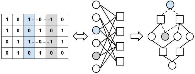
Figure 1: From left to right: binary matrix, bipartite graph and subgraph. Variable node and measurement node are denoted with circle and square, respectively. If two variable nodes share two same nonzero positions in their corresponding columns of binary matrix, they will form a shortest cycle of length 4 (dashed lines) in the subgraph expanded from each of them.

In this paper, we mainly study the regular binary matrix, which has the same number of nonzero entries in columns/rows. For notational simplicity, in the following work regular binary matrix is called binary matrix except for specific explanation. A given binary matrix can be uniquely associated with a bipartite graph, which consists of two classes of nodes, customarily called variable nodes and measurement nodes, corresponding to the columns and rows, respectively. A pair of variable and measurement nodes is connected by an edge if binary matrix has nonzero entry in the corresponding position. Hence, one can expand a subgraph from each variable node to connected nodes through edges. A closed path in subgraph is called a cycle. The length of the shortest cycle among all subgraphs is defined as the girth of the bipartite graph. One can derive that the value of the girth is even and not less than 4. For better understanding, we give an example in Figure 1. Note that sensing matrix is typically required to be normalized with columns. In this paper, assume that binary matrix has degree $d$, namely holding $d$ nonzero entries in each column, the nonzero entries are thus set to $1/\sqrt{d}$ instead of $1$.

To explore the potential sparsest sensing matrix, here we propose two critical definitions as shown in Definitions $1$ and $2$, which categorize the binary matrices into two classes in terms of girth distribution. Note that, the binary matrix with $g>4$ is preferred for LDPC codes as parity-check matrix, so its construction has been extensively studied in practice. In contrast, for the binary matrix with $g=4$, there is still no explicit way to construct a binary matrix with a given maximum correlation $s/d$, $2\leq s\leq d-1$. But recall that the nomarlized random binary matrix with uniform degree $d$, denoted as $R(M,N,d)$, is a typical binary matrix with $g=4$ while without specific constraint on the maximum correlation $s/d$. So in the following study, it is exploited as a practical version of the binary matrix with $g=4$.

Definition 1 (Binary matrix with girth $g>4$):  A binary matrix, denoted as $A(M,N,d)\in\{0,1/\sqrt{d}\}^{M\times N}$, consists of $2\leq d\leq M-2$ nonzero entries per column and $Nd/M$ nonzero entries per row. In the associated bipartite graph, the girth is required to be larger than $4$. Equivalently, any two distinct columns of this matrix are allowed to share at most one same nonzero position.

Definition 2 (Binary matrix with girth $g=4$):  A binary matrix, denoted as $A(M,N,d,s)\in\{0,1/\sqrt{d}\}^{M\times N}$, consists of $3\leq d\leq M-2$ nonzero entries per column and $Nd/M$ nonzero entries per row. In the associated bipartite graph, the girth takes value 4. Accordingly, the maximum correlation value between two distinct columns is $s/d$ with $2\leq s\leq d-1$.

It is known that the maximum correlation between distinct columns, denoted as $\mu$, has been a basic performance indicator for the sensing matrix [34]. So in the following Lemmas 1 and 2, we derive the correlation distributions of the binary matrices with $g>4$ and with $g=4$ (random binary matrix), respectively. It can be observed that the correlation distribution of the binary matrix with $g>4$ is simply binary, while the distribution of random binary matrix is relatively complicated. With the formula (7) for random binary matrix, it can be deduced that the probability of taking correlation value $s/d$ will significantly decrease as $s$ increases under the condition of $M\gg d$. This reveals that $\mu$ probably takes values much less than $1$, i.e. $s<<d$, such that the practical random binary matrix with limited columns has no same columns, . With the correlation characters shown in Lemmas 1 and 2, and the law that smaller $\mu$ leads to larger $k$ [34]:

$$k<\frac{1}{2}(1+1/\mu),$$ (5)

it is reasonable to expect that the binary matrix with $g>4$ probably approaches the best sensing performance, as $d$ achieves its upper bound. In the next Section, we further confirm this conjecture with RIP analysis.

Lemma 1 (Correlation distribution of binary matrix with $g>4$):   Any two distinct columns of binary matrix $A(M,N,d)$ with $g>4$ take correlation values as

$$a_{i}^{\prime}a_{j,j\neq i}=\left\{\begin{array}[]{cl}\textstyle 1/d&\textstyle\text{with probability}~{}\rho=\frac{Nd^{2}-Md}{(N-1)M}\\ \textstyle 0&\textstyle\text{with probability}~{}1-\rho\\ \end{array}\right.$$ (6)

where $a_{i}$ and $a_{j}$ denote two distinct columns of $A(M,N,d)$.

Proof:

In bipartite graph associated with $A(M,N,d)$, any variable node $v_{i}$, $i\in\{1,...,N\}$, holds $d$ neighboring measurement nodes $c_{b_{k}}$, where the subscript $b_{k}\in C\subset\{1,...,M\}$ denotes the index of measurement node, $k\in\{1,...,d\}$, $|C|=d$; each measurement node $c_{b_{k}}$ further connects with other $\frac{Nd}{M}-1$ variable nodes $v_{j}$, where $j\in V_{b_{k}}\subset\{1,...,N\}\setminus i$ represents the index of variable node, $|V_{b_{k}}|=\frac{Nd}{M}-1$. Since variable node $v_{i}$ has girth $g>4$, we have $V_{b_{e}}\bigcap V_{b_{f}}=\emptyset$, and then derive $|V_{b_{1}}\bigcup V_{b_{2}}\bigcup...\bigcup V_{b_{k}}|=d\times(\frac{Nd}{M}-1)$, where $e,f\in\{1,...,k\}$ and $e\neq f$. Therefore, among $N-1$ variable nodes, there are $\frac{Nd^{2}-Md}{M}$ connected to variable node $v_{i}$ through one measurement node. This reveals that any column of $A(M,N,d)$ has $\frac{Nd^{2}-Md}{M}$ correlated columns with correlation value $1/d$. Then the probability that any two distinct columns correlate to each other is derived as $\frac{Nd^{2}-Md}{(N-1)M}$ . ∎

Lemma 2 (Correlation distribution of random binary matrix with $g=4$):   Any two distinct columns of random binary matrix $R(M,N,d)$ take correlation values as

$$r_{i}^{\prime}r_{j,j\neq i}=s/d~{}~{}~{}\text{with probability}~{}\textstyle\rho=\frac{d!d!(M-d)!(M-d)!}{(d-s)!(d-s)!s!(M-2d+s)!M!}$$ (7)

where $r_{i}$ and $r_{j}$ denote two distinct columns, and $0\leq s\leq d$.

Proof:

The correlation between columns is determined by the overlap rate of nonzero positions of two columns. Assume that two columns have $s$ same nonzero positions, $0\leq s\leq d$, then the corresponding probability can be easily derived as

$$\textstyle\rho=\frac{C_{M}^{d-s}C_{M-(d-s)}^{d-s}C_{M-2(d-s)}^{s}}{C_{M}^{d}C_{M}^{d}}=\frac{d!d!(M-d)!(M-d)!}{(d-s)!(d-s)!s!(M-2d+s)!M!}$$

if $d$ nonzero positions are selected randomly and uniformly in each column of $R(M,N,d)$. ∎

III Near-optimal binary matrix for compressed sensing

In this section, the RIPs of binary matrices with $g>4$ and $g=4$ are first evaluated in Theorems $1$-$3$, and then the near-optimal binary matrix is derived with Theorem $4$ and related remarks.

III-A RIP of binary matrix with girth larger than 4

As sated before, RIP can be derived by searching the extreme eigenvalues of random symmetric matrix $A_{T}^{\prime}A_{T}$ with arbitrary $T\subset\{1,...,N\}$. In terms of Lemma 1 and the normalization of columns, we can easily derive that $A_{T}^{\prime}A_{T}\in\{0,1,1/d\}^{k\times k}$ has the diagonal equal to 1, and the corresponding off-diagonal holds binary distribution as shown in Lemma 1. With above given distribution, the extreme eigenvalues of $A_{T}^{\prime}A_{T}$ can be derived according to the algebraic algorithm [33]. Then the RIP is derived from Theorem 1.

Theorem 1 (RIP-1):   The binary matrix $A(M,N,d)$ with $g>4$ satisfies RIP with

$$\delta_{k}=\frac{3k-2}{4d+k-2}.$$ (8)

Proof:

Please see Appendix A.∎

Remark: From the proof of Theorem 1, it can be observed that the bounds of the two extreme eigenvalues are achieved only on the condition that the proportion p of nonzero entries in the off-diagonal of $A_{T}^{\prime}A_{T}$, could take value 1 or 0.5, for any $|T|$. However, as Lemma 1 discloses, this condition cannot be satisfied all the time, because with high probability the proportion $p$ should center on $\rho<1$ as $|T|$ increases. This is demonstrated by a real example in Figure 2, which shows the simulation results from a binary matrix $A(200,400,7)$ with $g>4$ constructed with PEG algorithm. As can be seen in Figure 2, the corresponding proportion $p$ will rapidly converge to the theoretical value $\rho=0.2281<0.5$, as $|T|$ increases. Therefore, for a large size binary matrix with $k$ large enough such that $p=\rho$, it is preferable to derive RIP with Wigner semicircle law [30], if the condition of $|T|\rightarrow\infty$ could also be approximately satisfied. The related RIP-2 is provided in Theorem 2. Note that, to obtain a relatively fair comparison, in the next Section we only adopt RIP-1 and RIP-3 which are derived with the same solution algorithm [33].

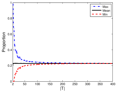
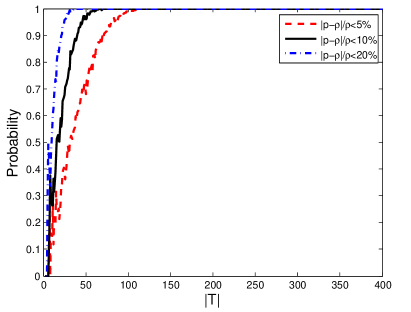
(a)                                                              (b)

Figure 2: (a) Maximum, mean and minimum of the proportion $p$ of nonzero entries in the off-diagonal of $A^{\prime}_{T}A_{T}$, for a real binary matrix $A(400,200,7)$ of $g>4$ constructed with PEG. As expected, the mean is equal to the theoretical value $\rho=0.2281$ derived with Lemma 1. (b) The probability that the proportion $p$ centers on the theoretical value $\rho$ within error bound $|p-\rho|/\rho$. Each point of (a) and (b) is derived from $10^{3}$ simulations.

Theorem 2 (RIP-2):   Assume that the off-diagonal elements of $A_{T}^{\prime}A_{T}$ take nonzero values with probability $\rho=\frac{Nd^{2}-Md}{(N-1)M}$ while $|T|(|T|-1)\rho\geq 2$, then the RIC of $A(M,N,d)$ can be approximately formulated as

$$\delta_{k}=\frac{k\rho+2\sqrt{k\rho(1-\rho)}+1}{k\rho-2\sqrt{k\rho(1-\rho)}+2d+1}$$ (9)

if $k=|T|\rightarrow\infty$.

Proof:

Please see Appendix B. ∎

III-B RIP of binary matrix with girth equal to 4

With the definition of binary matrix $A(M,N,d,s)$ with $g=4$, it is easy to derive that $A_{T}^{\prime}A_{T}$ has the maximum correlation of $\mu=s/d$, and the off-diagonal elements possibly drawn from the set $\{0,1/d,...,s/d\}$, where $3\leq d\leq M-2$ and $2\leq s\leq d-1$. By proceeding the proof similar with Theorem 1, the RIP of binary matrix with $g=4$ is obtained in Theorem 3.

Theorem 3 (RIP-3):  The binary matrix $A(M,N,d,s)$ with $g=4$ and $\mu=s/d$ , where $2\leq s\leq d-1$ and $3\leq d\leq M-2$, satisfies RIP with

$$\textstyle\delta_{k}=\left\{\begin{array}[]{ll}\Large{\frac{\textstyle(3k-2)s}{\displaystyle(k-2)s+4d}}&\footnotesize{if~{}~{}3\leq d\leq\frac{M}{2}~{}~{}and~{}~{}2\leq s\leq d-1}\\[10.0pt] \Large{\frac{\textstyle(3k-2)s+(k-2)(M-2d)}{\displaystyle(k-2)s-(M-2d)k+2M}}&\footnotesize{if~{}~{}\frac{M}{2}<d\leq M-2~{}~{}and~{}~{}2d-M\leq s\leq d-1}\\ \end{array}\right.$$ (10)

Proof:

Please see Appendix C.∎

Remark: Similar with RIP-1, the bounds of the two extreme eigenvalues for RIP-3 are achieved as the off-diagonal elements of $A_{T}^{\prime}A_{T}$ can take the maximum nonzero value $s/d$ with probability 1, or take binary value $\{0,s/d\}$ with equal probability. Unfortunately, two previous conditions cannot be ensured by a practical matrix which possibly takes $\mu=s/d$ with a relative low probability as Lemma 2 shows. This means that the RIP-3 cannot reasonably describe the RIP of the binary matrix that takes nonzero correlation values $1/d$ with high probability rather than $\{2/d,...,s/d\}$. In this case, its RIP is more close to RIP-1. Due to the inaccuracy of RIP-3, we have to specifically discuss this case in the following pursuit of the best sensing matrix.

III-C Near-optimal binary sensing matrix

According to the definition of binary matrix $A(N,M,d)$ with $g>4$, there is for the degree $d$, an upper bound denoted as $d_{max}$, which can be approximated as $d_{max}<\sqrt{M}<M/2$ with the inequality $1+d(\frac{dN}{M}-1)\leq N$ shown in [35]. From the Theorem 4 and related remarks, it can be observed that in theory there possibly exist three classes of binary matrices holding better RIP than the matrix $A(N,M,d_{max})$, while in fact only one of them can be practically constructed with slightly better RIP. Therefore, in this paper the matrix $A(N,M,d_{max})$ is viewed as the ’near-optimal’ binary sensing matrix, because it achieves nearly the best RIP with as sparse distribution as possible.

Theorem 4 (RIP of binary matrix $A(N,M,d_{max})$ ):   Among all binary matrices with $g\geq 4$ and $d\leq d_{max}$, the binary matrix $A(N,M,d_{max})$ holds the best RIP. Compared to the binary matrices with $g=4$ and $d>d_{max}$, the binary matrix $A(N,M,d_{max})$ also performs better under each of the following two conditions:

• $d_{max}\geq d/s$,  if $d_{max}<d\leq M/2$

• $d_{max}\geq\frac{(k+1)(2d-M)}{6s+2(2d-M)}$,  if $M/2<d\leq M-2$

where $d$, $s$ and $k$ follow the definitions of Theorems 1 and 3.

Proof:

We first prove that $A(M,N,d_{max})$ is the best one among all binary matrices with $g>4$, namely $A(M,N,d_{max})$ is better than $A(M,N,d)$ with $d\leq d_{max}$. With RIP-1, it is easy to derive that the RIC-$\delta_{k}$ decreases as the degree $d$ increases. Thus, it is proved that binary matrix with $g>4$ achieves best RIP as $d=d_{max}$.

Then, we are ready to prove that $A(M,N,d_{max})$ is still better than the binary matrix with $g=4$. Note that, the binary matrix with $g=4$ has degree $d$ possibly varying in the set $\{3,...,M-2\}$, and so in the following proof it is tailored into two parts ($d\leq d_{max}$ and $d>d_{max}$) for evaluation. For the case of $d\leq d_{max}$, by comparing RIP-1 and RIP-3, we can derive that $\frac{3k-2}{4d+k-2}<\frac{(3k-2)s}{(k-2)s+4d}$, if $2\leq s\leq d-1$ and $3\leq d\leq M/2$. This indicates that the RIC-$\delta_{k}$ of binary matrix with $g>4$ is less than that of binary matrix with $g=4$ under the same degree $d$. So considering $A(M,N,d_{max})$ is the best among all binary matrices with $g>4$, it also outperforms the binary matrix with $g=4$ and $d\leq d_{max}$. For the case of $d>d_{max}$, by comparing RIP-1 and RIP-3, it can be shown that $A(M,N,d_{max})$ performs better than the binary matrix with $g=4$ in the following two cases:

• $d_{max}\geq d/s$, derived with $\frac{3k-2}{4d_{max}+k-2}\leq\frac{(3k-2)s}{(k-2)s+4d}$ under $d_{max}<d\leq M/2$;

• $d_{max}\geq\frac{(k+1)(2d-M)}{6s+2(2d-M)}$, deduced from $\frac{3k-2}{4d_{max}+k-2}\leq\frac{(3k-2)s+(k-2)(M-2d)}{(k-2)s-(M-2d)k+2M}$ under $M/2<d\leq M-2$.

∎

Remark: According to Theorem 4, we know that there are two reverse conditions for which the binary matrix with $g=4$ will outperform the near-optimal matrix $A(M,N,d_{max})$. However, in practice it seems hard to construct such kind of matrices based on the observations below:

• For the reverse condition of $d>sd_{max}$, it seems hard to construct the binary matrix with a desired degree $d$. Indeed, based on the definition of $d_{max}$, it is known that $d\leq sd_{max}$ if $s=1$. Further, let $d^{\prime}=d_{max}+1$, and with the definition of binary matrix with $g=4$, the corresponding $s^{\prime}$ should take value from the set $\{2,...,d^{\prime}-1\}$ . In this case, it is easy to derive that that $d^{\prime}/s^{\prime}<d_{max}$. As for $d^{\prime}>d_{max}+1$, with Lemma 2, it can be observed that with high probability $s^{\prime}$ will take larger values as $d^{\prime}$ increases. Empirically, $s^{\prime}$ often increases much faster than $d^{\prime}$ during the practical matrix construction. Therefore it can be conjectured that $d^{\prime}/s^{\prime}<d_{max}$ when $d^{\prime}>d_{max}+1$.

• With the reverse condition of $d_{max}<\frac{(k+1)(2d-M)}{6s+2(2d-M)}$, it seems difficult to directly analyze or determine the binary matrix with desired degree $d$. But note that the reverse condition is derived on the assumption that $M/2<d\leq M-2$, which is out of our interest of searching the sparsest matrix in the context that sparse matrix can propose comparable performance with dense matrix.

Besides above two reverse cases, in fact, there remains a specific subclass of binary matrices with $g=4$, which possibly outperforms $A(M,N,d_{max})$. This type of matrices has degree $d$ slightly larger than $d_{max}$, such that the associated bipartite graph tends to hold relative few shortest cycles with length equal to 4, and equivalently with high probability the nonzero correlations between distinct columns thus take value $1/d$ ($<1/d_{max}$) rather than $\mu=s/d$ ($>1/d_{max}$), where $s$ is also slightly larger than 1. In this case, this type of matrices can be approximately regarded as the binary matrices with $g>4$ but $d$ ($>d_{max}$), and so they probably obtain better RIP than $A(M,N,d_{max})$. In practice, this type of matrices tends to occur at a relative small region, e.g., $d-d_{max}<3$ in our experiments, since with the observation on Lemma 2, the probability of taking correlation value $1/d$ will dramatically decrease as $d$ increases. This means that their performance gain over $A(M,N,d_{max})$ is relatively small, as can be seen from the following experiments. In addition, it is interesting to understand why this specific case is not disclosed in the proof of Theorem 4. As the remark of Theorem 3, this is because the RIP of the matrices with high probability taking correlation values $1/d$ rather than $\{2/d,...,s/d\}$, cannot be accurately described with RIP-3, such that they are ignored during the RIP comparison of Theorem 4.

Note that in this paper the binary matrix is evaluated only with the regular form. Similar conclusion can be expanded to the irregular binary matrix of uneven degrees, that is, the irregular matrix with larger average degree tends to have better RIP when $g>4$. Significantly, in practice the irregular matrix probably obtains better RIP than the regular matrix, since the former usually can be constructed with larger average degree than the latter under the constraint of $g>4$ [35].

IV Simulation results

IV-A Simulation setup

The proposed near-optimal binary sensing matrix $A(N,M,d_{max})$ is evaluated by comparing it with four types of matrices below:

• deterministic binary matrix with $g>4$ and $d<d_{max}$ constructed with PEG algorithm;

• deterministic binary matrix with $g=4$ and $d>d_{max}$ constructed with PEG algorithm;

• random binary matrix with uniform column degree;

• random Gaussian matrix.

Recall that up to now the binary matrix with $g=4$ and $\mu=s/d$ cannot be explicitly constructed. So here we exploit two typical binary matrices with $g=4$ while without specific constraint on $\mu$: the binary matrix with $g=4$ and $d>d_{max}$ constructed with PEG algorithm, and random binary matrix $R(M,N,d)$. For notational clarity, in the following part all binary matrices (with $g\geq 4$) constructed with PEG algorithm are denoted with $A(M,N,d)$. Gaussian matrix is referred as a performance baseline. Here PEG algorithm is adopted to construct the binary matrices with $g>4$ for the following two reasons. First, this greedy algorithm based on maximizing girth is suitable for approaching the $d_{max}$ of binary matrix with $g>4$ in terms of the fact that the girth $g$ will decrease dramatically as $d$ increases. Second, it can flexibly construct binary matrices with diverse degrees. However, due to the greediness, it should be noted that PEG algorithm cannot guarantee to obtain the theoretical $d_{max}$ in practice. For limited simulation time, here we only test the matrices of size (200, 400). For other matrix sizes, the interested readers may refer to the experimental results shown in [1]. Given the matrix size of (200, 400), the near-optimal matrix with $d_{max}=7$, namely $A(200,400,7)$, is determined with PEG algorithm.

The simulation exploits four representative decoding algorithms: orthogonal matching pursuit (OMP) algorithm [36] [37], iterative hard thresholding (IHT) algorithm [38], subspace pursuit (SP) algorithm [39] and basis pursuit (BP) algorithm [40]. Each simulation point is derived after $10^{4}$ iterations. Both binary random matrix and Gaussian matrix are randomly generated at each iteration. The sparse signal has nonzero entries drawn from $N(0,1)$. And the correct recovery rates are measured with $1-||\hat{x}-x||_{2}/||x||_{2}$.

IV-B Near-optimal performance over varying sparsity

TABLE I: The largest sparsity level $k$ that can be recovered with probability larger than $99\%$, for four classes of matrices: $A(200,400,d\leq 7)$ with $g>4$ (namely $A_{\ell}$), $A(200,400,d>7)$ with $g=4$ (namely $A_{e}$), random binary matrix $R(200,400,d)$ (namely $R$) and Gaussian random matrix of size (200,400) (namely $G$). The largest $k$ over varying $d$ is highlighted in bold. Recall that $A_{\ell}$ with $d=7$ denotes the proposed near-optimal matrix $A(200,400,7)$.

$d$			2	3	4	5	6	7	8	9	10	11	12	13	14	15	20	30	40	50	100
OMP	$k$	$A_{\ell}$	29	70	75	78	80	$\mathbf{81}$	-	-	-	-	-	-	-	-	-	-	-	-	-
		$A_{e}$	-	-	-	-	-	-	83	83	81	80	79	78	78	77	75	74	48	26	2
		$R$	0	55	69	73	75	76	76	76	76	76	76	76	76	76	76	76	76	76	76
		$G$	76
IHT	$k$	$A_{\ell}$	1	34	47	53	55	56	-	-	-	-	-	-	-	-	-	-	-	-	-
		$A_{e}$	-	-	-	-	-	-	57	55	53	50	48	47	45	44	37	27	16	7	1
		$R$	0	14	38	45	48	48	47	46	45	44	44	44	43	43	38	30	22	18	3
		$G$	53
SP	$k$	$A_{\ell}$	17	62	71	73	74	75	-	-	-	-	-	-	-	-	-	-	-	-	-
		$A_{e}$	-	-	-	-	-	-	75	74	74	73	72	71	71	77	71	70	25	9	1
		$R$	0	48	65	68	71	71	71	71	71	71	71	71	70	70	70	70	70	70	69
		$G$	73
BP	$k$	$A_{\ell}$	25	57	61	61	61	61	-	-	-	-	-	-	-	-	-	-	-	-	-
		$A_{e}$	-	-	-	-	-	-	62	61	59	59	58	58	57	57	54	51	36	18	1
		$R$	0	45	55	58	58	58	58	58	57	57	57	56	56	56	55	53	50	49	37
		$G$	63

The binary matrices of varying degree $d$ are evaluated by the maximum sparsity $k$ of sparse signal that can be correctly recovered with a rate over $99\%$. Obviously, larger $k$ indicates better performance. As performance reference, the maximum $k$ for Gaussian matrix is also provided. All results are shown in Table 1. For notational simplicity, in Table 1 the binary matrices $A(200,400,d)$ constructed with PEG algorithm are shortly denoted as $A_{\ell}$ and $A_{e}$ respectively for the cases $g>4$ and $g=4$; and random binary matrix $R(200,400,d)$ and Gaussian matrix are abbreviated to $R$ and $G$, respectively. Note that, for limited simulation time, we cannot enumerate all possible values of $d$. But clearly the results are sufficient to capture the performance varying tendency of tested matrices. With these results, first, it can be observed that the maximum $k$ follows the order: the near-optimal matrix $A(200,400,7)$ $>$Gaussian matrix$>$Random binary matrix $R(200,400,2\leq d\leq 100)$, except the unique case of Gaussian matrix$>$the near-optimal matrix$>$Random matrix under BP decoding. This demonstrates that the near-optimal matrix $A(200,400,7)$ outperforms random binary matrix. And then we turn to compare the near-optimal matrix $A(200,400,7)$ with other binary matrices $A(200,400,d)$ constructed with PEG. Among all binary matrices of $g>4$ (namely $A_{\ell}$ in the Table 1), clearly $A(200,400,7)$ is indeed the only case that can achieve the best performance simultaneously for above four decoding algorithms. Note that, although the matrices $A(200,400,d\in\{4,5,6\})$ achieve same $k$ with $A(200,400,7)$ under BP decoding, their correct decoding precisions in fact are less than the latter. However, compared with the cases of $g=4$ (namely $A_{e}$ in the Table 1), there are few cases obtaining comparable and even better performance than the proposed near-optimal case, such as $A(200,400,d\in\{8,9\}>d_{max}=7)$ under OMP and $A(200,400,d=8)$ under other three algorithms. With the former remarks of Theorem 4, these results can be explained by the fact that the aforementioned matrices $A(200,400,d\in\{8,9\})$ constructed with PEG, with high probability take nonzero correlation values as $1/d$ ($<1/d_{max}$) rather than as $\mu=s/d$ ($>1/d_{max}$), if $d-d_{max}$ is relatively small, so that they can be approximately regarded as the binary matrices with $g>4$ but $d>d_{max}$. Recall that PEG algorithm is designed to greedily reduce the increasing speed of the girth of bipartite graph as the degree $d$ of the binary matrix progressively increases. This yields that the correlation values of the constructed matrix largely center on $1/d$ rather than on $s/d$ with $s$ slightly larger than 1, when $d$ is slightly larger than $d_{max}$. With the results shown in Table 1 and [1], it is obvious that this type of matrices constructed with PEG algorithm lies in a relative small region, e.g. $d-d_{max}\leq 2$ in our simulations. Therefore they practically can be easily derived after the near-optimal binary matrix is determined. Overall, the proposed binary matrix indeed shows nearly the best performance with the highest sparsity.

Moreover, it is interesting to point out that the binary matrices constructed with PEG, $A(200,400,d<d_{max})$, still outperform random binary matrix and even Gaussian matrix for most decoding algorithms, if $d$ is slightly smaller than $d_{max}$, e.g. $d_{max}-d<3$ in our experiments. This allows us to practically construct the binary matrix with a more hardware-friendly structure [21], i.e. the quasi-cyclic structure, while preserving favorable performance in the negative case where the quasi-cyclic structure tends to slightly lower the value of $d_{max}$ [41] [21].

IV-C Performance over sparse signals of low sparsity or Gaussian noise

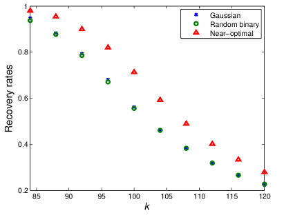
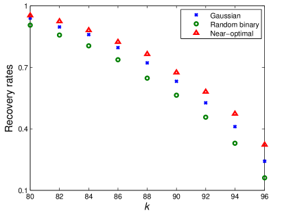
(a)                                                             (b)

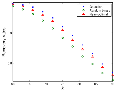
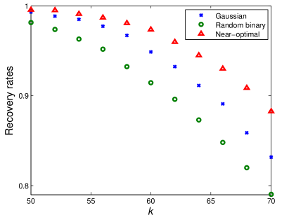
(c)                                                             (d)

Figure 3: The recovery rates of the near-optimal matrix $A(200,400,7)$, random binary matrix $R(200,400,7)$ and Gaussian matrix, over sparse signals of varying sparsity $k$. OMP in (a), SP in (b), BP in (c) and IHT in (d).

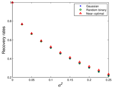
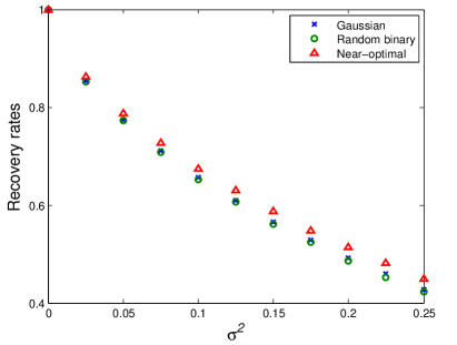
(a)                                                             (b)

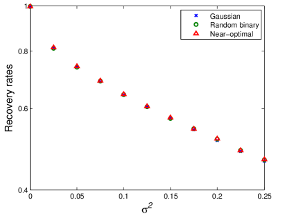
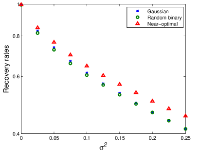
(c)                                                             (d)

Figure 4: The recovery rates of the near-optimal binary matrix $A(200,400,7)$, random binary matrix $R(200,400,7)$ and Gaussian matrix, over normalized sparse signals perturbed with Gaussian noise $N(0,\sigma^{2})$. OMP in (a), SP in (b), BP in(c) and IHT in(d).

This section evaluates the practical performance of the near-optimal matrix with sparse signal suffering from the following two potential challenges: 1) sparsity $k$ beyond the tolerance limit of sensing matrix; 2) additive Gaussian noise. Random binary matrix $R(200,400,7)$ and Gaussian matrix are also tested for comparison. The performance over sparse signals of excessive sparsity $k$ is illustrated in Figure 3. In Figure 4, we depict the influence of Gaussian noise $N(0,\sigma^{2})$ on normalized sparse signals of the sparsity $k=40$, which can be well decoded by three types of matrices as shown in Table 1, such that the following comparison under noises is fair. Similar with the results shown in Table 1, the proposed near-optimal matrix still shows better performance than other two types of matrices, except for the case of sparse signals of excessive $k$ with BP decoding, as shown in Figure 3(c), where it performs slightly worse than Gaussian matrix. In addition, due to the low performance resolution of Figure 4(c), it is necessary to point out that the near-optimal matrix also obtains tiny gains over other two competitors on the case of sparse signals of Gaussian noise decoded by BP.

V Conclusion

This paper has proposed the near-optimal distribution of binary sensing matrices through the analysis of RIP. In practice, the proposed matrix of expected performance can be approximately constructed with PEG algorithm. Specifically, it even shows better performance over Gaussian matrix with popular greedy decoding algorithms. As stated before, the term ’near-optimal’ is derived due to the fact that in practice there exists a class of matrices with sightly better RIP. These matrices hold degrees slightly larger than that of the near-optimal matrix, such that they can be easily found in practice. However, they are not formally defined in the literature since their structures are hard to be explicitly formulated. One must note that, as a sufficient condition, RIP is not an ideal tool for evaluating the performance of sensing matrices. So a more effective way is expected to be developed in the future to tackle this problem. In addition, it should be mentioned that the ideal degree of the proposed near-optimal matrix is only approximately bounded in this paper; and the practical construction algorithm, PEG algorithm, is also suboptimal due to its greediness. Consequently, it might be interesting in the future to further investigate the real degree of the proposed near-optimal matrix both in theory and practice.

Appendix A Proof of Theorem 1

Proof:

As stated before, the solution to RIC-$\delta_{k}$ can be reformulated as the pursuit for the extreme eigenvalues of random symmetric matrix $A_{T}^{\prime}A_{T}\in\{0,1,1/d\}^{k\times k}$, where $|T|=k$. Thus the following proof borrows the solution algorithm of extreme eigenvalues proposed in [33]. The eigenvalues of $A_{T}^{\prime}A_{T}$ are customarily denoted and ordered with $\lambda_{1}(A_{T}^{\prime}A_{T})\geq\ldots\geq\lambda_{k}(A_{T}^{\prime}A_{T})$ .

1. Let $B=A^{\prime}_{T}A_{T}-I\in\{0,1/d\}^{k\times k}$, then $B_{ii}=0$ and $B_{ij,i\neq j}=0$ or $1/d$.
   Let normalized $x=(x_{1},\ldots,x_{k})^{\prime}$ be the eigenvector corresponding to $\lambda_{k}(B)$. Then the minimal eigenvalue can be formulated as

   $$\lambda_{k}(B)=x^{\prime}Bx=\mathds{1}^{\prime}[B\circ(xx^{\prime})]\mathds{1}$$

   where $\circ$ denotes the Hadamard product and $\mathds{1}=(1,\ldots,1)^{\prime}\in\mathbb{R}^{k}$. Since $B$ is symmetric, by simultaneous permutations of the rows and columns of $B$, we can suppose $x_{i}\geq 0$ for $i=1,\ldots,n$ and $x_{i}<0$ for $i=n+1,\ldots,k$, and then $xx^{\prime}$ is divided into four parts:
   

   $$xx^{\prime}=\begin{bmatrix}X_{n\times n}&X_{n\times(k-n)}\\ X_{(k-n)\times n}&X_{(k-n)\times(k-n)}\end{bmatrix}$$

   where the entries in $X_{n\times n}$ and $X_{(k-n)\times(k-n)}$ are nonnegative, while the entries in $X_{n\times(k-n)}$ and $X_{(k-n)\times n}$ are nonpositive. Further, define a novel matrix $\tilde{B}$ of same size with $B$

   $$\tilde{B}=\begin{bmatrix}0\times\mathds{1}_{n\times n}&\frac{1}{d}\times\mathds{1}_{n\times(k-n)}\\ \frac{1}{d}\times\mathds{1}_{(k-n)\times n}&0\times\mathds{1}_{(k-n)\times(k-n)}\end{bmatrix}$$

   where $\mathds{1}_{a\times b}$ is an $a\times b$ matrix with all entries equal to $1$. It is easy to deduce that

   $$\lambda_{k}(\tilde{B})=\min\{y^{\prime}\tilde{B}y:\|y\|=1\}\leq x^{\prime}\tilde{B}x\leq x^{\prime}Bx=\lambda_{k}(B).$$

   Since the rank of $\tilde{B}$ is at most $2$, it has at most two nonzero eigenvalues. Considering the trace and the Frobenius norm, we have

   $$\lambda_{k}(\tilde{B})=-\sqrt{\frac{n(k-n)}{d^{2}}},~{}0\leq n\leq k.$$

   If $k$ is even, $\lambda_{k}(\tilde{B})\geq-\frac{k}{2d}$, with ’$=$’ at $n=k/2$.
   If $k$ is odd, $\lambda_{k}(\tilde{B})\geq-\frac{\sqrt{k^{2}-1}}{2d}$, with ’$=$’ at $n=(k-1)/2$ or $n=(k+1)/2$.
   Then $\lambda_{k}(B)\geq\lambda_{k}(\tilde{B})\geq-\frac{k}{2d}$, with the limitation attained at $k$ is even and $n=k/2$.

   So, we have the minimum eigenvalue $\lambda_{k}(A_{T}^{\prime}A_{T})\geq 1-\frac{k}{2d}$.

2. Let $C=A^{\prime}_{T}A_{T}-\frac{d-1}{d}\times I$, then $C_{ii}=1/d$ and $C_{ij,i\neq j}=0$ or $1/d$ .

   Let normalized $x=(x_{1},\ldots,x_{k})^{\prime}$ be the eigenvector corresponding to $\lambda_{1}(C)$. By simultaneous permutations of $C$ and $x$, we can suppose $x_{i}\geq 0$ for $i=1,\ldots,n$ and $x_{i}<0$ for $i=n+1,\ldots,k$, and the maximal eigenvalue is formulated as

   $$\lambda_{1}(C)=x^{\prime}Cx=\mathds{1}^{\prime}[C\circ(xx^{\prime})]\mathds{1}.$$

   Further define

   $$\tilde{C}=\begin{bmatrix}\frac{1}{d}\times\mathds{1}_{n\times n}&0\times\mathds{1}_{n\times(k-n)}\\ 0\times\mathds{1}_{(k-n)\times n}&\frac{1}{d}\times\mathds{1}_{(k-n)\times(k-n)},\end{bmatrix}$$

   then

   $$\begin{split}\lambda_{1}(\tilde{C})&=\max\{y^{\prime}\tilde{C}y:\|y\|=1\}\geq x^{\prime}\tilde{C}x\geq x^{\prime}Cx\\ &=\lambda_{1}(C).\end{split}$$

   Since the rank of $\tilde{C}$ is at most $2$, it has at most two nonzero eigenvalues. Considering the trace and the Frobenius norm, we have

   $$\lambda_{1}(\tilde{C})=\frac{k+|k-2n|}{2d}.$$

   Then $\lambda_{1}(C)\leq\lambda_{1}(\tilde{C})\leq\frac{k}{d}$, with ’$=$’ at $n=0$ or $n=k$. Thus, we can further derive

   $$\lambda_{1}(A_{T}^{\prime}A_{T})=\lambda_{1}(C)+\frac{d-1}{d}\leq\frac{k+d-1}{d}.$$

3. Finally, it follows from the results of both 1) and 2) that

   $$\delta_{k}=\frac{\lambda_{1}(A^{\prime}_{T}A_{T})-\lambda_{k}(A^{\prime}_{T}A_{T})}{\lambda_{1}(A^{\prime}_{T}A_{T})+\lambda_{k}(A^{\prime}_{T}A_{T})}=\frac{3k-2}{4d+k-2},$$

   with $\frac{\lambda_{1}(A^{\prime}_{T}A_{T})}{\lambda_{k}(A^{\prime}_{T}A_{T})}=\frac{1+\delta_{k}}{1-\delta_{k}}$ [42].

∎

Appendix B Proof of Theorem 2

Proof:

To derive the extreme eigenvalues of $A_{T}^{\prime}A_{T}$, we first search the extreme eigenvalues of

$$B=(A_{T}^{\prime}A_{T}-I)$$

where $I$ is an identity matrix. And clearly $B$ is a symmetric matrix of the diagonal elements equal to 0, and the off-diagonal elements equal to $1/d$ with property $\rho$ and 0 with property $1-\rho$.

With [43], suppose

$$Q=\frac{1}{\sqrt{\rho(1-\rho)}}(dB-\rho\mathds{1})$$

where $\mathds{1}$ is a all-ones matrix. Then $Q$ has entries with mean zero and variance one. With Wigner semicircle law [30], the extreme eigenvalues $\frac{1}{\sqrt{k}}Q$ with $k=|T|$, can be approximated as

$$-2\leq\lambda(\frac{1}{\sqrt{k}}Q)\leq 2$$

namely,

$$-2{\sqrt{k\rho(1-\rho)}}\leq\lambda(dB-\rho\mathds{1})\leq 2{\sqrt{k\rho(1-\rho)}},$$

if $k\rightarrow\infty$ [44].

With cauchy interlacing inequality [45], one can further derive

$$\lambda_{i}(dB-\rho\mathds{1})\leq\lambda_{i}(dB)\leq\lambda_{i-1}(dB-\rho\mathds{1})$$

for $1<i\leq k$, if $B-\rho\mathds{1}$ and $\rho\mathds{1}$ are Hermitian matrices, and $\rho\mathds{1}$ is positive semi-definite and has rank equal to 1. As a result, it is easy to derive that

$$\lambda_{2}(B)\leq\frac{1}{d}\cdot\lambda_{1}(dB-\rho\mathds{1})\leq\frac{2}{d}{\sqrt{k\rho(1-\rho)}}$$

and

$$\lambda_{k}(B)\geq\frac{1}{d}\cdot\lambda_{k}(dB-\rho\mathds{1})\geq-\frac{2}{d}{\sqrt{k\rho(1-\rho)}}$$

As for $\lambda_{1}(B)$ , it is known that [47]

$$\lambda_{1}(B)\approx\frac{1}{d}(k\rho+1).$$

In this sense, the extreme eigenvalues of $A_{T}^{\prime}A_{T}$ can be approximately formulated as

$$\lambda_{1}(A_{T}^{\prime}A_{T})=\lambda_{1}{B}+1\leq\frac{1}{d}(k\rho+1)+1$$

and

$$\lambda_{k}(A_{T}^{\prime}A_{T})=\lambda_{k}{B}+1\geq-\frac{2}{d}{\sqrt{k\rho(1-\rho)}}+1$$

Finally, the RIC of $A_{T}^{\prime}A_{T}$ is deduced as

$$\delta_{k}=\frac{\lambda_{1}-\lambda_{k}}{\lambda_{1}+\lambda_{k}}=\frac{k\rho+2\sqrt{k\rho(1-\rho)}+1}{k\rho-2\sqrt{k\rho(1-\rho)}+2d+1}$$

∎

Appendix C Proof of Theorem 3

The proof is similar to that for Theorem 1 in Appendix A. So in the following we just give a sketch.

Proof:

1. If $3\leq d\leq M/2$, $[A^{\prime}_{T}A_{T}]_{ii}=1$ and $[A^{\prime}_{T}A_{T}]_{ij,i\neq j}\in\{0,\ldots,s/d\}$, $2\leq s\leq d-1$, for $i,j=1,\ldots,k$.

   1. Let $B=A^{\prime}_{T}A_{T}-I$, derive

      $$\lambda_{k}(B)\geq\left\{\begin{array}[]{ll}-sk/2d&if~{}k~{}is~{}even\\[6.0pt] -s\sqrt{k^{2}-1}/2d&if~{}k~{}is~{}odd\\ \end{array}\right.,$$

      and then

      $$\lambda_{k}(A^{\prime}_{T}A_{T})=1+\lambda_{k}(B)\geq 1-\frac{sk}{2d}.$$

   2. Let $C=A^{\prime}_{T}A_{T}-(1-\frac{s}{d})I$, derive $\lambda_{1}(C)\leq ks/d$, and then

      $$\lambda_{1}(A^{\prime}_{T}A_{T})\leq\frac{(k-1)s+d}{d}.$$

2. if $M/2<d\leq M-1$, $[A^{\prime}_{T}A_{T}]_{ii}=1$ and $[A^{\prime}_{T}A_{T}]_{ij,i\neq j}$ $\in\{(2d-M)/d,\ldots,s/d\}$, $2d-M\leq s\leq d-1$, for $i,j=1,\ldots,k$.

   1. Let $B=A^{\prime}_{T}A_{T}-(1-\frac{2d-M}{d})I$, derive

      $$\lambda_{k}(B)\geq\left\{\begin{array}[]{ll}\frac{k(2d-M-s)}{2d}&\footnotesize{if~{}k~{}is~{}even}\\[6.0pt] \frac{k(2d-M)-\sqrt{(2d-M)^{2}-(k^{2}-1)s^{2}}}{2d}&\footnotesize{if~{}k~{}is~{}odd}\\ \end{array}\right.,$$

      
      

      further deduce $\lambda_{k}(B)\geq-\frac{k(2d-M-s)}{2d}$, and then we have that

      $$\lambda_{k}(A^{\prime}_{T}A_{T})\geq\frac{k(2d-M-s)+2(M-d)}{2d}$$

   2. Let $C=A^{\prime}_{T}A_{T}-(1-\frac{s}{d})I$, derive $\lambda_{1}(C)\leq ks/d$, and then it follows that
      

      $$\lambda_{1}(A^{\prime}_{T}A_{T})\leq\frac{(k-1)s+d}{d}.$$

3. Finally, it follows from $\delta_{k}=\frac{\lambda_{1}-\lambda_{k}}{\lambda_{1}+\lambda_{k}}$ that
   
   

   $$\large{\delta_{k}}=\left\{\begin{array}[]{ll}\frac{\textstyle(3k-2)s}{\textstyle(k-2)s+4d}&\footnotesize{if~{}3\leq d\leq\frac{M}{2}}~{}and~{}\footnotesize{2\leq s\leq d-1}\\[12.0pt] \frac{\textstyle(3k-2)s+(k-2)(M-2d)}{\textstyle(k-2)s-(M-2d)k+2M}&\footnotesize{if~{}\frac{M}{2}<d\leq M-2}~{}and~{}\footnotesize{2d-M\leq s\leq d-1}\\ \end{array}\right.$$

∎

References

- [1] W. Lu, K. Kpalma, and J. Ronsin, “Sparse binary matrices of LDPC codes for compressed sensing,” in Data Compression Conference (DCC), 2012, april 2012, p. 405.
- [2] E. Candes and T. Tao, “Decoding by linear programming,” IEEE Transactions on Information Theory, vol. 51, no. 12, pp. 4203–4215, dec. 2005.
- [3] ——, “Near-optimal signal recovery from random projections: Universal encoding strategies?” IEEE Transactions on Information Theory, vol. 52, no. 12, pp. 5406–5425, Dec. 2006.
- [4] D. Achlioptas, “Database-friendly random projections: Johnson–Lindenstrauss with binary coins,” J. Comput. Syst. Sci., vol. 66, no. 4, pp. 671–687, 2003.
- [5] R. Baraniuk, M. Davenport, R. DeVore, and M. Wakin, “A simple proof of the restricted isometry property for random matrices,” Constructive Approximation, vol. 28, no. 3, pp. 253–263, 2008.
- [6] R. Berinde and P. Indyk, “Sparse recovery using sparse random matrices,” MIT-CSAIL Technical Report, 2008.
- [7] N. Ailon and E. Liberty, “Fast dimension reduction using rademacher series on dual bch codes,” in Proceedings of the nineteenth annual ACM-SIAM symposium on Discrete algorithms, 2008, pp. 1–9.
- [8] A. Amini and F. Marvasti, “Deterministic construction of binary, bipolar, and ternary compressed sensing matrices,” IEEE Transactions on Information Theory, vol. 57, no. 4, pp. 2360 –2370, april 2011.
- [9] M. Akcakaya and V. Tarokh, “A frame construction and a universal distortion bound for sparse representations,” IEEE Transactions on Signal Processing, vol. 56, no. 6, pp. 2443–2450, june 2008.
- [10] S. Howard, A. Calderbank, and S. Searle, “A fast reconstruction algorithm for deterministic compressive sensing using second order reed-muller codes,” in 42nd Annual Conference on Information Sciences and Systems (CISS 2008), march 2008, pp. 11–15.
- [11] R. Calderbank, S. Howard, and S. Jafarpour, “Sparse reconstruction via the reed-muller sieve,” in 2010 IEEE International Symposium on Information Theory Proceedings (ISIT), 2010, pp. 1973–1977.
- [12] ——, “Construction of a large class of deterministic sensing matrices that satisfy a statistical isometry property,” IEEE Journal of Selected Topics in Signal Processing, vol. 4, no. 2, pp. 358–374, 2010.
- [13] H. Pham, W. Dai, and O. Milenkovic, “Sublinear compressive sensing reconstruction via belief propagation decoding,” in IEEE International Symposium on Information Theory, 2009, pp. 674–678.
- [14] A. Barg and A. Mazumdar, “Small ensembles of sampling matrices constructed from coding theory,” in IEEE International Symposium on Information Theory Proceedings (ISIT),, 2010, pp. 1963–1967.
- [15] P. Indyk, “Explicit constructions for compressed sensing of sparse signals,” in Proceedings of the nineteenth annual ACM-SIAM symposium on Discrete algorithms, 2008, pp. 30–33.
- [16] R. A. DeVore, “Deterministic constructions of compressed sensing matrices,” Journal of Complexity, vol. 23, no. 4-6, pp. 918–925, 2007.
- [17] W. Xu and B. Hassibi, “Efficient compressive sensing with deterministic guarantees using expander graphs,” in IEEE Information Theory Workshop, ITW ’07, sept. 2007, pp. 414 –419.
- [18] S. Jafarpour, W. Xu, B. Hassibi, and R. Calderbank, “Efficient and robust compressed sensing using optimized expander graphs,” IEEE Transactions on Information Theory, vol. 55, no. 9, pp. 4299–4308, 2009.
- [19] A. Dimakis, R. Smarandache, and P. Vontobel, “LDPC codes for compressed sensing,” IEEE Transactions on Information Theory, vol. 58, no. 5, pp. 3093 –3114, may 2012.
- [20] D. Li, X. Liu, S. Xia, and Y. Jiang, “A class of deterministic construction of binary compressed sensing matrices,” Journal of Electronics (China), vol. 29, pp. 493–500, 2012.
- [21] X. Liu and S. Xia, “Construction of Quasi-Cyclic Measurement Matrices Based on Array Codes,” in IEEE International Symposium on Information Theory, Jul. 2013.
- [22] R. Tanner, “A recursive approach to low complexity codes,” IEEE Transactions on Information Theory, vol. 27, no. 5, pp. 533–547, 1981.
- [23] ——, “Minimum-distance bounds by graph analysis,” Information Theory, IEEE Transactions on, vol. 47, no. 2, pp. 808–821, 2001.
- [24] M. Sipser and D. Spielman, “Expander codes,” IEEE Transactions on Information Theory, vol. 42, no. 6, pp. 1710 –1722, Nov 1996.
- [25] B. L. Sturm, “Sparse vector distributions and recovery from compressed sensing,” arXiv:1103.6246, Jul. 2011.
- [26] D. Needell and J. A. Tropp, “Cosamp: iterative signal recovery from incomplete and inaccurate samples,” Commun. ACM, vol. 53, no. 12, pp. 93–100, Dec. 2010.
- [27] A. M. Tillmann and M. E. Pfetsch, “The Computational Complexity of the Restricted Isometry Property, the Nullspace Property, and Related Concepts in Compressed Sensing,” arXiv:1205.2081, May 2012.
- [28] A. S. Bandeira, E. Dobriban, D. G. Mixon, and W. F. Sawin, “Certifying the restricted isometry property is hard,” arXiv:1204.1580, Apr. 2012.
- [29] J. D. Blanchard, C. Cartis, and J. Tanner, “Compressed sensing: How sharp is the restricted isometry property?” SIAM Rev., vol. 53, no. 1, pp. 105–125, Feb. 2011.
- [30] L. Pastur, “On the spectrum of random matrices,” Theoretical and Mathematical Physics, vol. 10, pp. 67–74, 1972.
- [31] S. Gurevich and R. Hadani, “The statistical restricted isometry property and the wigner semicircle distribution of incoherent dictionaries,” arXiv:0812.2602, Dec. 2008.
- [32] R. Horn and C. Johnson, Matrix Analysis. Cambridge University Press, 1985.
- [33] X. Zhan, “Extremal eigenvalues of real symmetric matrices with entries in an interval,” SIAM Journal on Matrix Analysis and Applications, vol. 27, no. 3, pp. 851–860, 2005.
- [34] D. Donoho and X. Huo, “Uncertainty principles and ideal atomic decomposition,” IEEE Transactions on Information Theory, vol. 47, no. 7, pp. 2845–2862, Nov 2011.
- [35] X.-Y. Hu, E. Eleftheriou, and D. Arnold, “Regular and irregular progressive edge-growth Tanner graphs,” IEEE Transactions on Information Theory, vol. 51, no. 1, pp. 386 –398, jan. 2005.
- [36] Y. Pati, R. Rezaiifar, and P. Krishnaprasad, “Orthogonal matching pursuit: recursive function approximation with applications to wavelet decomposition,” in Conference Record of The Twenty-Seventh Asilomar Conference on Signals, Systems and Computers, nov. 1993, pp. 40–44 vol.1.
- [37] J. A. Tropp and A. C. Gilbert, “Signal recovery from random measurements via orthogonal matching pursuit,” IEEE Transaction on Information Theory, vol. 53, pp. 4655–4666, 2007.
- [38] T. Blumensath and M. E. Davies, “Iterative hard thresholding for compressed sensing,” Applied and Computational Harmonic Analysis, vol. 27, no. 3, pp. 265–274, 2009.
- [39] W. Dai and O. Milenkovic, “Subspace pursuit for compressive sensing signal reconstruction,” IEEE Transactions on Information Theory, vol. 55, no. 5, pp. 2230–2249, 2009.
- [40] S. Boyd and L. Vandenberghe, Convex Optimization. Cambrige university press, March 2004.
- [41] Z. Li and B. Kumar, “A class of good quasi-cyclic low-density parity check codes based on progressive edge growth graph,” in Conference Record of the Thirty-Eighth Asilomar Conference on Signals, Systems and Computers, vol. 2, 2004, pp. 1990–1994.
- [42] S. Foucart and M.-J. Lai, “Sparsest solutions of underdetermined linear systems via -minimization for ,” Applied and Computational Harmonic Analysis, vol. 26, no. 3, pp. 395 – 407, 2009.
- [43] L. V. Tran, V. H. Vu, and K. Wang, “Sparse random graphs: Eigenvalues and eigenvectors,” Random Structures & Algorithms, vol. 42, no. 1, pp. 110–134, 2013.
- [44] Z. Füredi and J. Komlós, “The eigenvalues of random symmetric matrices,” Combinatorica, vol. 1, pp. 233–241, 1981.
- [45] T. Tao and V. Vu, “Random matrices: Universality of local eigenvalue statistics,” Acta Mathematica, vol. 206, pp. 127–204, 2011.
- [46] T. Ando, Y. Kabashima, H. Takahashi, O. Watanabe, and M. Yamamoto, “Spectral analysis of random sparse matrices,” IEICE Transactions, pp. 1247–1256, 2011.
- [47] Y. Kabashima, H. Takahashi, and O. Watanabe, “Cavity approach to the first eigenvalue problem in a family of symmetric random sparse matrices,” Journal of Physics: Conference Series, vol. 233, no. 1, p. 012001.