The Effective Temperature Scale of M dwarfs

Abstract

Context. Despite their large number in the Galaxy, M dwarfs remain elusive objects and the modeling of their photospheres has long remained a challenge (molecular opacities, dust cloud formation).

Aims. Our objectives are to validate the BT-Settl model atmospheres, update the M dwarf $T_{\mathrm{eff}}$-spectral type relation, and find the atmospheric parameters of the stars in our sample.

Methods. We compare two samples of optical spectra covering the whole M dwarf sequence with the most recent BT-Settl synthetic spectra and use a $\chi^{2}$ minimization technique to determine $T_{\mathrm{eff}}$. The first sample consists of 97 low-resolution spectra obtained with NTT at La Silla Observatory. The second sample contains 55 mid-resolution spectra obtained at the Siding Spring Observatory (SSO). The spectral typing is realized by comparison with already classified M dwarfs.

Results. We show that the BT-Settl synthetic spectra reproduce the slope of the spectral energy distribution and most of its features. Only the CaOH band at 5570Å and AlH and NaH hydrides in the blue part of the spectra are still missing in the models. The $T_{\mathrm{eff}}$-scale obtained with the higher resolved SSO 2.3 m spectra is consistent with that obtained with the NTT spectra. We compare our $T_{\mathrm{eff}}$-scale with those of other authors and to published isochrones using the BT-Settl colors. We also present relations between effective temperature, spectral type and colors of the M dwarfs.

1 Introduction

Low-mass stars of less than 1 M_⊙ are the dominant stellar component of the Milky Way. They constitute 70% of all stars (Reid & Gizis, 1997, Bochanski et al. 2010) and 40% of the total stellar mass of the Galaxy (Chabrier, 2003, 2005). Our understanding of the Galaxy therefore relies upon the description of this faint component. Indeed, M dwarfs have been employed in several Galactic studies as they carry the fundamental information regarding the stellar physics, galactic structure and its formation and dynamics. Moreover, M dwarfs are now known to host exoplanets, including super-Earth exoplanets (Bonfils et al., 2007, 2012, Udry et al. 2007). The determination of accurate fundamental parameters for M dwarfs has therefore relevant implications for both stellar and Galactic astronomy. Because of their intrinsic faintness and difficulties in getting homogeneous samples with respect to age and metallicity, their physics is not yet well understood.

Their atmosphere has been historically complex to model with the need for computed and ab initio molecular line lists accurate and complete to high temperatures. But for over ten years already, water vapor (Partridge & Schwenke, 1997, Barber et al. 2006) and titanium oxide (Plez, 1998) line lists, the two most important opacities in strength and spectral coverage, have become available meeting these conditions. And indeed, the PHOENIX model atmosphere synthetic spectral energy distribution improved greatly from earlier studies (Allard & Hauschildt, 1995, Hauschildt et al. 1999) to the more recent models by Allard et al. (2001, 2011, 2012a) and by Witte et al. (2011) using the most recent water vapor opacities.

The $T_{\mathrm{eff}}$-scale of M dwarfs remain to this day model-dependent to some level. Many efforts have been made to derive the effective temperature scale of M dwarfs. Due to the lack of very reliable model atmosphere, indirect methods such as blackbody fitting techniques have historically been used to estimate the effective temperature. The Bessell (1991) $T_{\mathrm{eff}}$-scale was based on black-body fits to the near-IR (JHKL) bands by Pettersen (1980) and Reid & Gilmore (1984). The much cooler black-body fits shown from Wing & Rinsland (1979) and Veeder (1974) were fits to the optical. Their fitting line was a continuation of the empirical $T_{\mathrm{eff}}$ relation for the hotter stars through the Pettersen (1980) and Reid & Gilmore (1984) IR fits for the cooler stars. The work by Veeder (1974), Berriman & Reid (1987), Berriman et al. (1992) and Tinney et al. (1993) also used the blackbody fitting technique to estimate the $T_{\mathrm{eff}}$. Tsuji et al. (1996a) provide good $T_{\mathrm{eff}}$ using infrared flux method (IRFM). Casagrande et al. (2008) provides a modified IRFM $T_{\mathrm{eff}}$ for dwarfs including M dwarfs. These methods tend to underestimate $T_{\mathrm{eff}}$ since the blackbody carries little flux compared to the M dwarfs in the Rayleigh Jeans tail redwards of $2.5\leavevmode\nobreak\ \mu$m. Temperature derived from fitting to model spectra (Kirkpatrick et al., 1993) are systematically $\sim$ 300  K warmer than those empirical methods. These cooler $T_{\mathrm{eff}}$-scale for M dwarfs was corrected recently by Casagrande & Schönrich (2012) bring it close to the Bessell (1991, 1995) $T_{\mathrm{eff}}$-scale.

Tinney & Reid (1998) determined an M dwarf $T_{\mathrm{eff}}$-scale in the optical by ranking the objects in order of TiO, VO, CrH and FeH equivalent widths. Delfosse et al. (1999) pursued a similar program in the near-infrared (hereafter NIR) with H₂O indices. Tokunaga & Kobayashi (1999) used a spectral color index based on moderate dispersion spectroscopy in the K band. Leggett et al. (1996) used observed NIR low resolution spectra and photometry to compare with the AMES-Dusty models (Allard et al., 2001). They found radii and effective temperature which are consistent with the estimates based on photometric data from interior model or isochrone results. Leggett et al. (1998, 2000) revised their results by comparing the spectral energy distribution and NIR colors of M dwarfs to the same models. Their study provided for the first time a realistic temperature scale of M dwarfs.

In this paper, we present a new version of the BT-Settl models using the TiO line list by (Plez, 1998, and B. Plez, private communication) which is an important update since TiO accounts for the most important features in the optical spectrum. Compared to the version presented in Allard et al. (2012a) that was using Asplund et al. (2009) solar abundances, this new BT-Settl model uses also the latest solar elemental abundances by Caffau et al. (2011). We compare the revised BT-Settl synthetic spectra with the observed spectra of 152 M dwarfs using spectral synthesis and $\chi^{2}$ minimization techniques, and color-color diagrams to obtain the atmospheric parameters (effective temperature, surface gravity and metallicity). We determine the revised effective temperature scale along the entire M dwarfs spectral sequence and compare these results to those obtained by many authors. Observations and spectral classification are presented in section 2. Details of the the model atmospheres are described in section  3 and the $T_{\mathrm{eff}}$ determination is explained in section 4. The comparison between observations and models is done in section 5 where spectral features and photometry are compared. The effective temperature scale of M dwarfs is presented in this section. Conclusions are given in section 6.

2 Observations

We carried out spectroscopic observations on the 3.6m New Technology Telescope (NTT) at La Silla Observatory (ESO, Chile) in November 2003. Optical low-resolution spectra were obtained in the Red Imaging and Low-dispersion spectroscopy (RILD) observing mode with the EMMI instrument. The spectral dispersion of the grism we used is 0.28 nm/pix, with a wavelength range 385-950 nm. We used an order blocking filter to avoid the second order overlap that occurs beyond 800 nm. Thus the effective wavelength coverage ranges from 520 to 950 nm. The slit was 1 arcsec wide and the resulting resolution was 1 nm. The seeing varied from 0.5 to 1.5 arcsec. Exposure time ranged from 15 s for the brightest to 120 s for the faintest dwarf ($I$ = 15.3). The reduction of the spectra was done using the context long of MIDAS. Fluxes were calibrated with the spectrophotometric standards LTT 2415 and Feige 110.

We obtained spectra for 97 M dwarfs along the entire spectral sequence. They are presented in Reylé et al. (2006); Phan-Bao et al. (2005); Crifo et al. (2005); Martín et al. (2010). The list of stars, their spectral types and their optical and NIR photometry are given in Table 1. The photometry has been compiled using the Vizier catalog access through the Centre de Données astronomiques de Strasbourg. It comes from the NOMAD catalogue (Zacharias et al., 2005), the Deep Near-Infrared Survey (DENIS, Epchtein, 1997), the Two Micron All Sky Survey (2MASS, Skrutskie et al., 2006), Reid et al. (2004, 2007), Koen & Eyer (2002); Koen et al. (2010).

The observations of 55 additional M dwarfs at Siding Spring Observatory (hereafter SSO) were carried out using the Double Beam Spectrograph (DBS) that uses a dichroic beamsplitter to separate the blue (300–630 nm) and red (620–1000 nm) light. The blue camera with a 300 l/mm grating provided a 2 pixel resolution of 0.4 nm and the red camera with a 316 l/mm grating provided a 2 pixel resolution of 0.37 nm. The detectors were E2V 2048x512 13.5 micron/pixel CCDs. The observations were taken on Mar 27 2008. The spectrophotometric standards used were HD44007, HD45282, HD55496, HD184266, and HD187111 from the STIS Next Generation Spectral Library (NGSL, version 1), and L745-46a and EG131 from http://www.mso.anu.edu.au/$\sim$bessell/FTP/Spectrophotometry/. The list of stars with their photometry are given in table 2.

Spectral types for the NTT sample are obtained by visual comparison with a spectral template of comparison stars, observed together with the targets stars at NTT as explained in Reylé et al. (2006). For comparison, we also derive spectral types using the classification scheme based on the TiO and CaH bandstrength (Reid & Gizis, 1997). However no comparison stars have been observed with the DBS at SSO. Thus spectral types for the SSO sample are computed from TiO and CaH bandstrength. Although the instrument is different, we allow to use the comparison stars observed with EMMI on the NTT as a final check. The results agree within 0.5 subclass.

Table 1: Observable and physical quantities for our sample of stars observed at NTT with EMMI.

Name	Spectral Type	$T_{\mathrm{eff}}$	$T_{\mathrm{eff}}$ b	log g	$V$	$R$	$I$	$J$	$H$	$K$
		(K)	(K)	($cms^{-2}$)
Gl143.1a	K7	3900	—	5.0	10.03	9.15	—	—	—	—
LHS141	M0	3900	—	5.0	10.15	9.35	8.38	7.36	6.76	6.58
LHS3833a	M0.5	3800	—	5.0	10.06	9.33	—	—	—	—
HD42581a	M1	3700	—	5.0	8.12	7.16	6.12	—	—	—
LHS14a	M1.5	3600	—	5.0	10.04	9.09	7.99	—	—	—
LHS65a	M1.5	3600	3567	5.0	10.86	10.31	10.64	—	—	—
L127-33	M2	3500	—	5.0	14.19	14.04	12.41	11.17	10.58	10.32
NLTT10708	M2	3500	—	5.0	11.16	10.31	9.17	7.86	7.28	6.98
LP831-68	M2	3500	—	5.0	11.02	10.02	8.80	7.61	6.95	6.69
NLTT83-11	M2	3500	—	5.0	12.90	12.25	11.00	9.68	9.01	8.78
APMPMJ0541-5349	M2	3500	—	5.0	13.30	12.84	11.77	10.64	10.17	9.89
LHS1656	M2.5	3400	—	5.0	13.30	12.44	10.75	9.52	8.94	8.65
LP763-82	M2.5	3400	—	5.0	12.19	11.25	9.86	8.55	7.97	7.69
LP849-55	M2.5	3400	—	5.0	13.32	13.25	11.48	9.97	9.36	9.14
LHS5090	M3	3300	—	5.0	—	14.97	12.85	11.58	11.04	10.84
LHS3800	M3	3300	—	5.0	—	—	12.23	10.93	10.39	10.15
LHS3842	M3	3300	—	5.0	13.80	12.95	11.30	9.88	9.29	9.04
LHS1293	M3	3300	—	5.0	13.65	12.66	11.36	9.94	9.35	9.07
LP994-114	M3	3300	—	5.0	—	11.59	10.36	9.00	8.37	8.15
LTT9783	M3	3300	—	5.0	—	12.11	10.56	9.17	8.59	8.34
LP715-39	M3	3300	3161	5.0	12.65	11.53	10.09	8.67	8.11	7.82
LHS1208a	M3	3300	—	5.0	9.85	8.97	—	—	—	—
LEHPM4417	M3	3300	—	5.0	13.73	13.06	11.37	10.09	9.43	9.20
LP831-45	M3.5	3200	3125	5.0	12.54	11.51	9.90	8.49	7.88	7.62
2MASSJ04060688-0534444	M3.5	3200	—	5.0	13.29	12.28	—	9.13	8.55	8.30
LP834-32	M3.5	3200	3108	5.0	12.38	11.24	9.74	8.24	7.65	7.41
LHS502a	M3.5	3200	—	5.0	11.49	10.43	9.11	—	—	—
LEHPM 1175	M3.5	3200	—	5.0	—	13.08	11.51	10.01	9.47	9.17
LEHPM1839	M3.5	3200	—	5.0	—	13.32	12.11	10.55	9.95	9.71
L130-37	M3.5	3200	—	5.0	13.04	11.97	10.37	8.94	8.34	8.01
LEHPM6577	M3.5	3200	—	5.0	—	13.03	11.79	10.34	9.73	9.47
L225-57	M4	3200	—	5.0	—	11.70	9.79	8.23	7.61	7.31
LP942-107	M4	3200	3052	5.0	13.93	12.73	11.13	9.63	9.08	8.77
LP772-8	M4	3200	—	5.0	14.11	13.43	11.52	10.05	9.48	9.20
LP1033-31	M4	3200	—	5.0	—	12.12	10.54	9.10	8.46	8.21
L166-3	M4	3200	—	5.0	—	12.76	11.33	9.83	9.28	9.00
LP877-72	M4	3200	—	5.0	—	11.—	10.22	8.86	8.24	8.00
LP878-73	M4	3200	—	5.0	14.55	14.22	12.63	10.86	10.27	10.00
LP987-47	M4	3200	—	5.0	—	—	10.82	9.41	8.78	8.55
LP832-7	M4	3200	—	5.0	14.09	13.45	—	9.87	9.24	8.98
LHS183	M4	3200	—	5.0	12.79	11.51	—	8.57	8.00	7.75
LHS1471	M4	3200	—	5.0	—	13.22	11.56	9.94	9.37	9.08
APMPMJ2101-4125	M4	3200	—	5.0	—	13.34	11.47	9.96	9.38	9.09
APMPMJ2101-4907	M4	3200	—	5.0	—	—	10.52	9.12	8.48	8.19
LEHPM3260	M4	3200	—	5.0	—	12.53	10.60	9.13	8.54	8.19
LEHPM3866	M4	3200	—	5.0	—	—	11.82	10.21	9.58	9.29
LEHPM5810	M4	3200	—	5.0	—	13.58	11.66	9.91	9.33	9.05
LHS5045	M4.5	3100	—	5.0	—	—	10.78	9.17	8.60	8.24
LP940-20	M4.5	3100	—	5.0	—	14.87	12.65	10.92	10.32	10.01
L170-14A	M4.5	3100	—	5.0	—	12.86	11.50	9.76	9.13	8.88
LHS1201	M4.5	3100	—	5.0	17.55	15.52	12.90	11.12	10.52	10.25
LHS1524	M4.5	3100	—	5.0	—	14.45	12.65	10.98	10.45	10.17
LTT1732	M4.5	3100	—	5.0	—	13.19	11.27	9.69	9.11	8.80
LP889-37	M4.5	3100	2923	5.0	14.52	13.21	11.46	9.77	9.16	8.82
LHS5094	M4.5	3100	—	5.0	14.02	12.72	10.97	9.30	8.72	8.41
LP655-43	M4.5	3100	2924	5.0	14.44	13.14	11.41	9.73	9.14	8.82
LHS138a	M4.5	3100	—	5.0	12.07	10.70	8.94	—	—	—
APMPMJ1932-4834	M4.5	3100	—	5.0	—	14.38	12.37	10.63	10.02	9.72
2MASSJ23522756-3609128	M4.5	3100	—	5.0	—	17.27	—	13.09	12.57	12.28
LEHPM640	M4.5	3100	—	5.0	17.74	14.26	12.30	10.76	10.14	9.90
LEHPM1853	M4.5	3100	—	5.0	—	12.77	11.03	9.46	8.85	8.61
LEHPM3115	M4.5	3100	—	5.0	—	13.94	12.10	10.49	9.92	9.63
LEHPM4771	M4.5	3100	—	5.0	17.74	13.79	11.29	9.54	8.95	8.63
LEHPM4861	M4.5	3100	—	5.0	—	13.28	11.75	10.13	9.60	9.34
L291-115	M5	2900	—	5.0	15.88	14.90	12.26	10.44	9.83	9.54
LP904-51	M5	2900	—	5.0	—	15.32	12.84	11.04	10.44	10.16
LHS168	M5	2900	—	5.0	13.78	12.60	—	8.77	8.21	7.83

Table 1. Continued.
Name Spectral Type $T_{\mathrm{eff}}$ $T_{\mathrm{eff}}$ ^b log g $V$ $R$ $I$ $J$ $H$ $K$ (K) (K) ($cms^{-2}$) LP829-41 M5.5 2800 — 5.0 16.10 15.95 13.21 11.31 10.76 10.40 LP941-57 M5.5 2800 — 5.0 — 14.88 12.98 11.06 10.47 10.13 LHS546 M5.5 2800 — 5.0 14.69 — — 9.15 8.50 8.18 LP714-37 M5.5 2800 — 5.5 16.26 15.02 12.99 11.01 10.37 9.92 LHS1326 M6 2800 — 5.5 15.61 14.49 — 9.84 9.25 8.93 2MASSJ12363959-1722170 M6 2800 — 5.0 17.56 15.86 13.91 11.67 11.09 10.71 2MASSJ21481595-1401059 M6.5 2700 — 5.0 — 20.20 17.15 14.68 14.11 13.65 2MASSJ05181131-3101519 M6.5 2700 — 5.0 17.74 16.85 14.17 11.88 11.23 10.90 LP788-1 M6.5 2700 — 5.0 — 16.66 13.36 11.07 10.47 10.07 APMPMJ1251-2121 M6.5 2700 — 5.0 — 16.65 13.78 11.16 10.55 10.13 APMPMJ2330-4737 M7 2700 — 5.0 — — 13.70 11.23 10.64 10.28 LP789-23 M7 2700 — 5.0 — 17.90 14.55 12.04 11.39 10.99 LHS292 M7 2700 — 5.5 15.60 14.40 11.25 8.86 8.26 7.93 2MASSJ03144011-0450316 M7.5 2600 — 5.0 — 19.43 — 12.64 12.00 11.60 LHS1604 M7.5 2600 — 5.0 18.02 16.52 13.75 11.30 10.61 10.23 LP714-37 M7.5 2600 — 5.5 16.26 15.52 12.99 11.01 10.37 9.92 LP655-48 M7.5 2600 2250 5.0 17.86 15.95 13.35 10.66 9.99 9.54 LP851-346 M7.5 2600 — 5.5 — 16.79 13.77 10.93 10.29 9.88 LHS1367 M8 2600 — 5.0 — 17.34 14.18 11.62 10.95 10.54 2MASSJ05022640-0453583 M8 2600 — 5.0 — 20.39 17.35 14.52 13.95 13.58 LHS132 M8 2600 — 5.0 — 17.14 13.83 11.13 10.48 10.07 2MASSJ22062280-2047058 M8 2600 — 5.0 — 18.93 15.09 12.37 11.69 11.31 2MASSJ22264440-7503425 M8 2600 — 5.0 — 18.95 15.20 12.35 11.70 11.25 2MASSJ04103617-1459269 M8.5 2500 — 5.5 — — 16.68 13.94 13.24 12.81 2MASSJ05084947-1647167 M8.5 2500 — 5.5 — — 16.46 13.69 12.96 12.53 2MASSJ04362788-4114465 M8.5 2500 — 5.5 — 19.96 16.04 13.10 12.43 12.05 2MASSJ10481463-3956062 M9 2500 — 5.5 — 15.93 12.67 9.54 8.90 8.45 2MASSJ20450238-6332066 M9.5 2500 — 5.5 — 19.24 16.05 12.62 11.81 11.21 2MASSJ09532126-1014205 M9.5 2500 — 5.5 — 19.58 16.82 13.47 12.64 12.14

^a Saturation in NIR bands.
^b $T_{\mathrm{eff}}$ from Casagrande et al. (2008).

Table 2: Observable and physical quantities for our sample of stars observed at SSO.

Name	Spectral Type	$T_{\mathrm{eff}}$	$T_{\mathrm{eff}}$ b	log g	$V$	$R$	$I$	$J$	$H$	$K$
		(K)	(K)	($cms^{-2}$)
HIP49986	M1.5	3700	3445	5.0	9.07	8.21	7.08	5.89	5.26	5.01
HIP82256	M1.5	3700	3470	5.0	11.38	10.39	9.24	8.04	7.48	7.22
HIP56528	M1.5	3600	3472	5.0	9.81	8.85	7.66	6.47	5.86	5.62
NLTT19190	M1.5	3600	3456	5.0	11.49	10.57	9.34	8.11	7.47	7.20
NLTT42523	M2	3600	3444	5.0	12.08	11.06	9.81	8.60	8.01	7.80
HIP80229	M2	3600	3486	5.0	11.91	10.90	9.65	8.48	7.87	7.64
LP725-25	M2	3600	3476	5.0	11.76	10.82	9.59	8.36	7.68	7.44
HIP61413	M2	3500	3454	5.0	11.49	10.48	9.17	7.99	7.37	7.15
LP853-34	M2	3500	3339	5.0	12.32	11.31	9.99	8.69	8.10	7.83
LP859-11	M2	3500	3433	5.0	12.00	10.97	9.69	8.49	7.88	7.63
LP788-49	M2	3500	3356	5.0	11.81	10.85	9.55	8.30	7.74	7.49
HIP42762	M2	3500	3302	5.0	11.75	10.76	9.42	8.12	7.49	7.28
HIP51317	M2	3500	3403	5.0	9.67	8.67	7.34	6.18	5.60	5.31
HIP60559	M2	3500	3382	5.0	11.30	10.29	8.99	7.73	7.25	6.95
HIP47103	M2	3500	3319	5.0	10.87	9.89	8.58	7.34	6.74	6.47
HIP93206	M2.5	3500	3366	5.0	11.23	10.18	8.80	7.52	6.93	6.70
LP834-3	M2.5	3500	—	5.0	—	—	—	—	—	—
HIP84521	M2.5	3500	3345	5.0	11.57	10.53	9.22	7.93	7.39	7.11
HIP91430	M2.5	3500	3352	5.0	11.32	10.26	8.92	7.66	7.06	6.85
HIP50341	M2.5	3500	3314	5.0	11.02	10.01	8.62	7.32	6.71	6.45
LP672-2	M2.5	3400	—	5.0	12.58	11.54	10.12	8.80	8.14	7.93
NLTT24892	M2.5	3400	3244	5.0	12.52	11.47	10.05	8.73	8.118	7.84
NLTT34577	M2.5	3400	3254	5.0	12.44	11.40	9.99	8.64	8.00	7.80
LP670-17	M3	3400	3226	5.0	12.14	11.08	9.63	8.28	7.68	7.39
HIP59406	M3	3400	3226	5.0	11.75	10.69	9.25	7.89	7.36	7.04
HIP74190	M3	3400	3258	5.0	11.55	10.48	9.05	7.72	7.13	6.86
NLTT46868	M3.5	3400	3221	5.0	12.23	11.08	9.61	8.26	7.73	7.44
HIP62452	M4	3300	3095	5.0	11.46	10.31	8.71	7.19	6.67	6.36
NLTT25488	M4	3200	2986	5.0	15.66	14.46	12.73	11.09	10.52	10.21
NLTT29087	M4	3200	2971	5.0	14.79	13.57	11.84	10.22	9.62	9.35
NLTT29790	M4	3200	2987	5.0	14.73	13.54	11.85	10.22	9.64	9.34
LP734-32	M4	3200	3024	5.0	12.15	10.99	9.35	7.77	7.14	6.86
LP739-2	M4	3100	2939	5.0	14.44	13.18	11.40	9.73	9.17	8.89
LP735-29	M4	3100	2940	5.0	14.18	12.95	11.18	9.52	8.97	8.67
GJ1123	M4	3100	—	5.0	13.14	11.90	10.10	8.33	7.77	7.45
GJ1128	M4	3100	—	5.0	12.66	11.40	9.61	7.95	7.38	7.04
NLTT35266	M4.5	3100	2942	5.0	15.15	13.88	12.05	10.41	9.94	9.66
NLTT41951	M4.5	3100		5.0	15.06	13.77	11.99	10.36	9.80	9.51
NLTT21329	M4.5	3000	2949	5.0	13.75	12.38	10.42	8.60	8.07	7.73
LP732-35	M5	3100	2901	5.0	14.10	12.78	10.94	9.36	8.76	8.49
NLTT18930	M5	3100	2903	5.0	15.34	13.93	12.03	10.31	9.76	9.44
2MASS J14221943-7023371	M5	3000	—	5.0	—	—	—	—	—	—
NLTT22503	M5	3000	2785	5.0	13.66	12.32	10.39	8.50	7.92	7.60
NLTT28797	M5	3000	2826	5.0	15.62	14.24	12.32	10.54	9.99	9.64
NLTT30693	M5.5	3000	2785	5.5	15.32	13.86	11.85	9.95	9.36	9.00
LHS288	M5.5	3000	2770	5.0	13.87	12.42	10.31	8.48	8.05	7.73
GJ551	M5.5	2900	—	5.0	3.63	2.08	5.36	4.83	4.38	—
LHS2502	M6	2900	2468	5.5	19.36	17.54	15.33	12.75	12.07	11.79
NLTT20726	M6.5	2800	2464	5.0	16.11	14.24	11.85	9.44	8.84	8.44
GJ406	M6.5	2800	—	5.5	13.57	11.81	9.51	7.08	6.48	6.08
LHS2351	M7	2800	2346	5.5	19.22	17.39	14.91	12.33	11.72	11.33
SCR J1546-5534	M7.5	2700	—	5.5	—	—	—	—	—	—
GJ752b	M8	2700	—	5.5	5.01	—	—	9.91	9.23	8.76
GJ644c	M7	2700	—	5.5	16.90	14.78	12.24	9.78	9.20	8.82
LHS2397a	M8	2700	—	5.5	19.66	17.42	14.86	11.93	11.23	10.73
b $T_{\mathrm{eff}}$ from Casagrande et al. (2008).

3 Model atmospheres

For this paper, we use the most recent BT-Settl models partially published in a review by Allard et al. (2012a) and described by Allard & Homeier (2012). These model atmospheres are computed with the PHOENIX multi-purpose atmosphere code version 15.5 (Hauschildt et al., 1997, Allard et al. 2001) solving the radiative transfer in 1D spherical symmetry, with the classical assumptions: hydrostatic equilibrium, convection using the Mixing Length Theory, chemical equilibrium, and a sampling treatment of the opacities. The models use a mixing length as derived by the Radiation HydroDynamic (hereafter RHD) simulations of Ludwig et al. (2002, 2006) and Freytag et al. (2012) and a radius as determined by the Baraffe et al. (1998) interior models as a function of the atmospheric parameters ($T_{\mathrm{eff}}$, log $g$, [M/H]). The BT-Settl grid extends from $T_{\mathrm{eff}}=300-7000$ K, log$g=2.5-5.5$ and [M/H]$=-2.5-0.0$ accounting for alpha element enrichment. The reference solar elemental abundances used in this version of the BT-Settl models are those defined by Caffau et al. (2011). The synthetic colors and spectra are distributed with a spectral resolution of around R=100000 via the PHOENIX web simulator.

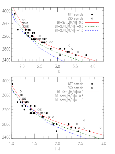
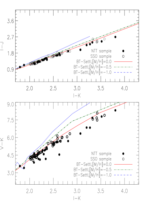
Figure 1: $T_{\mathrm{eff}}$ vs near-infrared colors (left panel) and color-color plot (right panel) for observed M dwarfs (open and filled circle) compared to the values obtained with the 5 Gyrs isochrones from Baraffe et al. (1998) at various metallicities.

Hot temperature grains have been shown to form in the uppermost layers of M dwarfs with effective temperatures below 3000 K, but clear effects observable at the spectral resolution considered in this paper are only apparent below 2600 K i.e. for later spectral type than those considered in this paper. These grains produce a ”veiling” by dust scattering over the optical band of the latest type M dwarfs. The BT-Settl models use therefore a slightly revised version of the Rossow (1978) cloud model. See Allard et al. (2012a, b), Allard & Homeier (2012) and Rajpurohit et al. (2012) for details on the model construction.

Relative to previous models by Allard et al. (2001), the current version of the BT-Settl model atmosphere is using the BT2 water vapor line list computed by Barber et al. (2006), TiO, VO, CaH line lists by Plez (1998), MgH by (Weck et al., 2003, Story et al. 2003), FeH and CrH by (Dulick et al., 2003, Chowdhury et al. 2006), NH₃ by Yurchenko et al. (2011), CO₂ (Tashkun et al., 2004), and H₂ Collision Induced Absorption (CIA) by Borysow et al. (2001) and Abel et al. (2011), to mention the most important. We use the CO line list by Goorvitch & Chackerian (1994a, b). Detailed profiles for the alkali lines are also used (Allard et al., 2007).

In general, the Unsold (1968) approximation is used for the atomic damping constants with a correction factor to the widths of 2.5 for the non-hydrogenic atoms (Valenti & Piskunov, 1996). More accurate broadening data for neutral hydrogen collisions by Barklem et al. (2000) have been included for several important atomic transitions such as the alkali, Ca I and Ca II resonance lines. For molecular lines, we have adopted average values (e. g. $\langle\gamma_{6}^{HIT}(T_{0},P_{0})\rangle_{H_{2}O}=0.08\,\,P_{\rm gas}\,[\mathrm{cm}^{-1}\mathrm{atm}^{-1}]$ for water vapor lines) from the HITRAN database (Rothman et al., 2009), which are scaled to the local gas pressure and temperature

$$\gamma_{6}(T)=\langle\gamma_{6}^{HIT}(T_{0},P_{0})\rangle\left(\frac{296\,K}{T}\right)^{0.5}\,\left(\frac{P}{1\,{\rm atm}}\right)\enspace,$$ (1)

with a single temperature exponent of 0.5, to be compared to values ranging mainly from 0.3 to 0.6 for water transitions studied by Gamache et al. (1996). The HITRAN database gives widths for broadening in air, but Bailey & Kedziora-Chudczer (2012) find that these agree in general within 10 – 20% with those for broadening by a solar composition hydrogen-helium mixture.

4 $T_{\mathrm{eff}}$ determination

We use a least-square minimization program using the new BT-Settl model atmospheres to derive a revised effective temperature scale of M dwarfs. The stars in our samples most probably belong to the thin disc of our Galaxy (Reylé et al., 2002; Reylé & Robin, 2004). Thus we determine the $T_{\mathrm{eff}}$ of our targets assuming solar metallicity. This is a reasonable assumption as can be seen in Fig. 1 where we compare our two samples to three 5 Gyrs isochrones with solar, [M/H]= -0.5 and -1.0 dex. The samples are clearly compatible with solar metallicity.

Both theory and observation indicate that M dwarfs have log $g\leavevmode\nobreak\ =\leavevmode\nobreak\ 5.0\pm 0.2$ (Gizis, 1996; Casagrande et al., 2008) except for the latest-type M dwarfs. We therefore restrict our analysis to log $g\leavevmode\nobreak\ =\leavevmode\nobreak\ 5.0-5.5$ models. Each synthetic spectrum was convolved to the observed spectral resolution a scaling factor is applied to normalize the average flux to unity. We then compare each of the observed spectra with all the synthetic spectra in the grid by taking the difference between the flux values of the synthetic and observed spectra at each wavelength point. We interpolated the model spectra on the wavelength grid of the observed spectra. The sum of the squares of these differences is obtained for each model in the grid, and the best model for each object is selected. The best models were finally inspected visually by comparing them with the corresponding observed spectra. Due to the lower signal-to-noise ratio in the SSO 2.3 m spectra bluewards of 500 nm (see Fig. 3), especially for spectral types later than M4, we have excluded this region below 500 nm from the $\chi^{2}$ computation. We have also checked the variation in effective temperature of the best fit as a function of the spectral type of the observed dwarfs. We found generally good agreement and conclude that our model fitting procedure can be used to estimate the effective temperature with an uncertainty of $\sim$100 K. The purpose of this fit is to determine the effective temperature by fitting the overall shape of the optical spectra. No attempt has been made to fit the individual atomic lines such as the K I and Na I resonance doublets. With the available resolution we cannot constrain the metallicity; high resolution spectra would be necessary (Rajupurohit et al. in prep.). In addition, we checked the influence of the spectral resolution to our derived temperatures. We degraded the resolution of the spectra of SSO 2.3 m down to 1 nm and redid the procedure. No systematic difference in $T_{\mathrm{eff}}$ was found. The results are summarized in Table 1 and  2.

5 Comparison between models and observations

5.1 Spectroscopic confrontation

The optical spectrum of M dwarfs is dominated by molecular band absorption, leaving no window onto the continuum (Allard, 1990). The major opacity sources in the optical regions are due to titanium oxide (TiO) and vanadium oxide (VO) bands, as well as to MgH, CaH, FeH hydrides bands and CAOH hydroxide bands in late-type M dwarfs. In M dwarfs of spectral type later than M6, the outermost atmospheric layers fall below the condensation temperature of silicates, giving rise to the formation of dust clouds (Tsuji et al., 1996a, b, Allard et al. 1997).

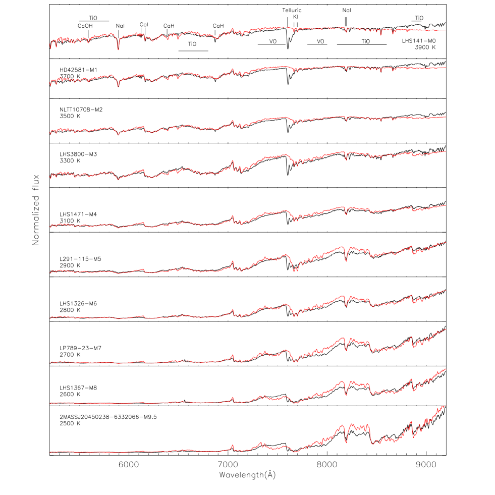
Figure 2: Optical to red SED of M dwarfs from M0 to M9.5 observed with the NTT at a spectral resolution of 10.4 Å compared to the best fit BT-Settl synthetic spectra (red lines). The models displayed have a surface gravity of log $g$ = 5.0 to 5.5. Telluric features near 7600 Å have been ignored from the chi-square minimization.

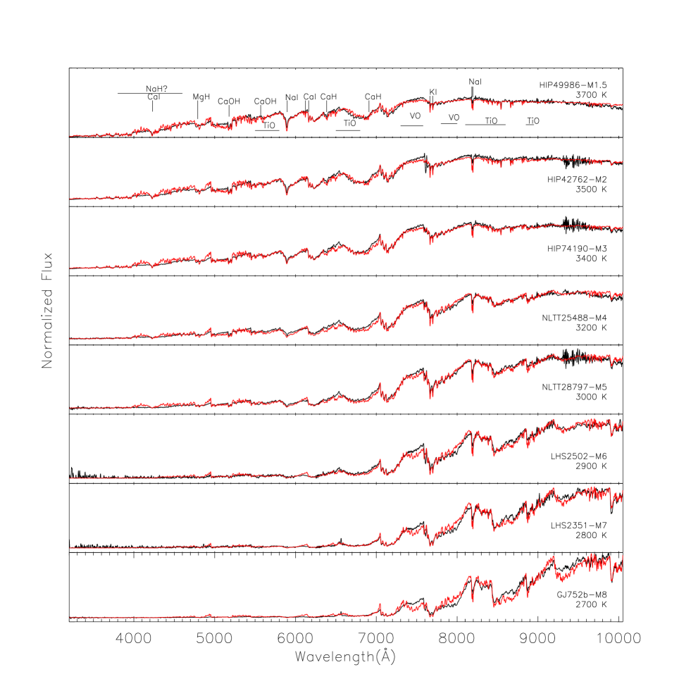
Figure 3: Optical to red SED of M dwarfs from M1 to M8 observed with the SSO 2.3 m at a spectral resolution of 1.4 Å compared to the best fitting (chi-square minimization) BT-Settl synthetic spectra (red lines). The models displayed have a surface gravity of log $g$=5.0 to 5.5. At blue wavelengths ($<$ 5000$\AA$) the instrumentals noise dominate the late-type M dwarfs.

We compared the two samples of M dwarfs with the most recent BT-Settl synthetic spectra in Fig. 2 and 3 through the entire M dwarf spectral sequence. The synthetic spectra reproduce very well the slope of the observed spectra across the M dwarfs regime. This is a drastic improvement compared to previous comparisons of earlier models (e.g. Leggett et al., 1998).

However, some indications of missing opacities persist in the blue part of the late-type M dwarf such as the B’ ²$\Sigma$⁺$<$– X ²$\Sigma$⁺ system of MgH (Skory et al., 2003), as well as TiO and VO opacities around 8200 Å. Opacities are totally missing for the CaOH band at 5570 Å. The missing hydride bands of AlH and NaH between 3800 and 4600 Å among others could be responsible for the remaining discrepancies. Note that chromospheric emission fills the Na I D transitions in the latest-type M dwarfs displayed here.

We see in this spectral regime no signs of dust scattering or of the weakening of features due to sedimentation onto grains until the M8 and later spectral types where the spectrum becomes flat due to the sedimentation of TiO and VO bands and to the veiling by dust scattering.

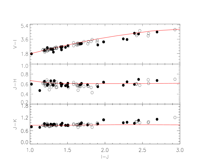
(a)

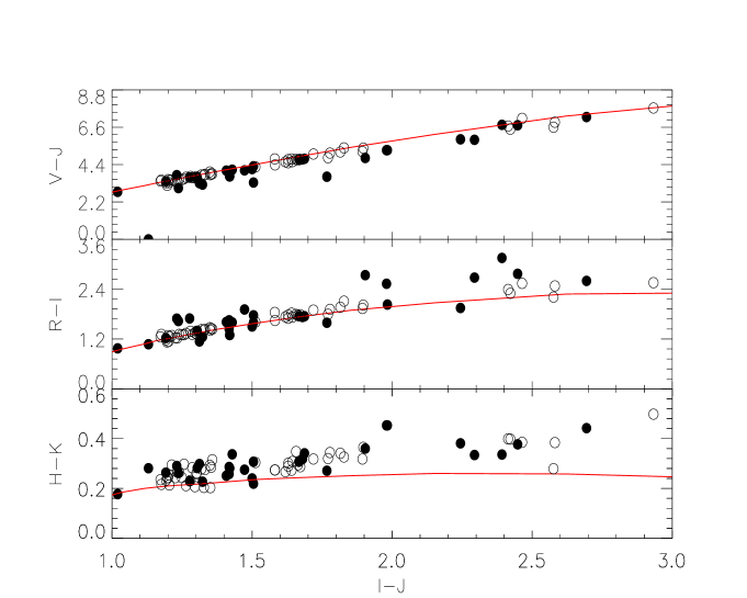
(b)

Figure 4: Optical and NIR colors obtained with the 5 Gyrs isochrones from Baraffe et al. (1998) at solar metallicity compared with the two observation samples (filled circles for the NTT sample and open circle for the SSO 2.3 m spectra). Typical error bars are comparable or smaller than the size of the symbols.

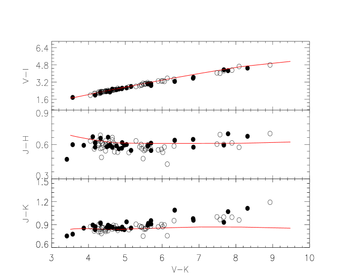
(c)

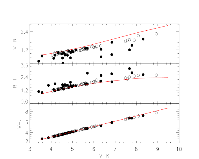
(d)

Figure 4: Continued.

5.2 Photometric confrontation

The models can be validated by comparing published isochrones interpolated into the new BT-Settl synthetic color tables with observed photometry. We have taken the log g and $T_{\mathrm{eff}}$ for the fixed age of 5 Gyrs from Baraffe et al. (1998) isochrones and calculated the colors of the star according to the BT-Settl models. . The models are compared to observations in color-color diagrams in Fig.  4 for our two samples. The compiled photometry in the NTT sample is less homogeneous, translating to a larger spread in particular for colors including the $V$ and $R$-band. This dispersion becomes dramatical for the coolest, and faintest, stars.

except for lowest mass objects at very young ages. The isochrone reproduces the two samples over the entire M dwarf spectral range in most colors. In particular, the models reproduce the $V$-band colors of M dwarfs, as illustrated by the $V-I$, $V-J$ and $V-K$ colors. An increasing offset to the latest types persists in the $H-K$ and $V-R$ color indices. The observations suggest also a flattening and possibly a rise in $J-H$ and $J-K$ to the latest types which is not reproduced by the model. These inadequacies at the coolest temperature could be linked to missing opacities.

5.3 The $T_{\mathrm{eff}}$-scale of M dwarfs

The effective temperature scale versus spectral type is shown in Fig. 5. The $T_{\mathrm{eff}}$-scale determined using the NTT sample (filled circles) is in agreement with the SSO sample (filled triangles) but we found systematically 100 K higher $T_{\mathrm{eff}}$ for SSO sample for spectral type later than M5. The relation shows a saturation trend for spectral types later than M8. This illustrate the fact that the optical spectrum no longer change sensibly with $T_{\mathrm{eff}}$ in this regime due to dust formation.

In the following we compare our scale to other works. Bessell (1991) determined the temperatures by comparing blackbodies to the NIR photometry of their sample. They used the temperature calibration of Wing & Rinsland (1979) and Veeder (1974). These calibrations were identical between $2700\leq T_{\mathrm{eff}}\leq 3500\,K$. Their scale agrees with the modern values for M dwarfs earlier than M6, but becomes gradually too cool with later spectral type and too hot for earlier M types.

Leggett et al. (1996) used the Base grid by Allard & Hauschildt (1995) covering the range of parameter down to the coolest known M dwarfs, M subdwarfs and brown dwarfs. They obtained the $T_{\mathrm{eff}}$ of M dwarfs by comparing the observed spectra to the synthetic spectra. They perform their comparison independently at each of their four wavelength regions: red, $J$, $H$, and $K$. The different wavelength regions gave consistent values of $T_{\mathrm{eff}}$ within 300 K. Gizis (1997) used the NextGen model atmosphere grid by Allard et al. (1997). These models include more molecular lines from ab initio simulations (in particular for water vapor) than the previous Base model grid. Leggett et al. (2000) used the more modern AMES-Dusty model atmosphere grid by Allard et al. (2001). They obtained a revised $T_{\mathrm{eff}}$ scale which is 150-200 K cooler for early-Ms, and 200 K hotter for late-Ms than the scale presented in Fig. 5. Testi (2009) determine the $T_{\mathrm{eff}}$ by fitting the synthetic spectra to the observations. They used three classes of models: the AMES-Dusty, AMES-Cond and the BT-Settl models. With some individual exceptions they found that the BT-Settl models were the most appropriate for M type and early L-type dwarfs.

Finally, for spectral type later than M0, Luhman et al. (2003) adopted the effective temperature which is based on the NextGen and AMES-Dusty evolutionary models of Baraffe et al. (1998) and Chabrier et al. (2000) respectively. They obtained the $T_{\mathrm{eff}}$ by comparing the H-R diagram from theoretical isochrones of Baraffe et al. (1998) and Chabrier et al. (2000). For M8 and M9, Luhman et al. (2003) adjusted the temperature scale from Luhman (1999) so that spectral sequence fall parallel to the isochrones. Their $T_{\mathrm{eff}}$ conversion is likely to be inaccurate at some level, but as it falls between the scales for dwarfs and giants, the error in $T_{\mathrm{eff}}$ are modest.

The different $T_{\mathrm{eff}}$ scales are in agreement within 250-300 K. But the Gizis (1997) relation shows the largest differences, with the largest $T_{\mathrm{eff}}$-values (up to 500 K). This is due to the incompleteness of the TiO and water vapor line lists used in the NextGen model atmospheres. Note also how the Luhman et al. (2003) $T_{\mathrm{eff}}$ scale is gradually overestimating $T_{\mathrm{eff}}$ towards the bottom of the main sequence for spectral types later than M4.

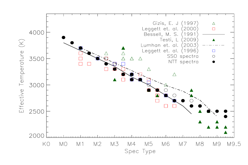
Figure 5: Spectral type - $T_{\mathrm{eff}}$ relation obtained with the NTT sample (filled circles) and the SSO 2.3 m sample (open circles) compared to relations by Bessell (1991), Gizis (1997), Leggett et al. (1996), Leggett et al. (2000), Testi (2009), and Luhman (1999).

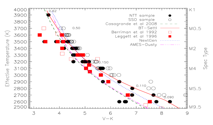
(a)

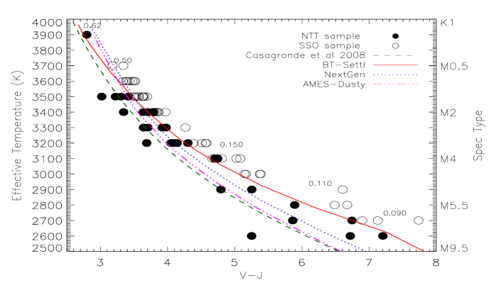
(b)

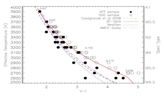
(c)

Figure 6: Color-$T_{\mathrm{eff}}$ plots in different bands from the NTT sample (filled circles) and the SSO 2.3 m sample (open circles). Spectral types are also indicated. The predictions from BT-Settl (solid line), NextGen (dotted line) and AMES-Dusty (das-dotted) for solar metallicities are over plotted. Theoretical masses in solar mass are indicated. Predictions from other authors are shown for comparison when available.

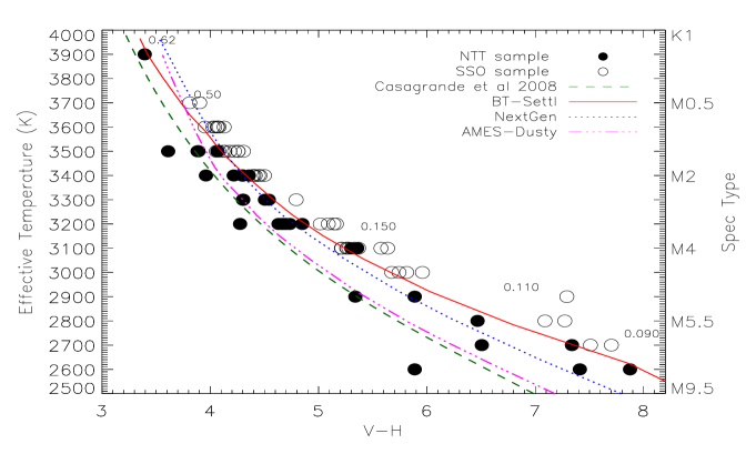
(d)

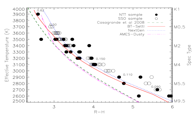
(e)

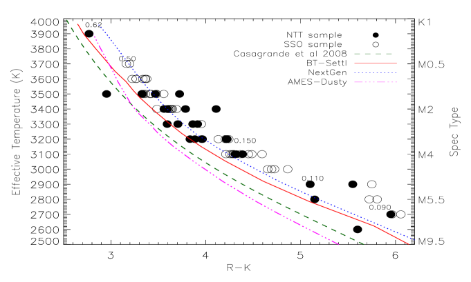
(f)

Figure 6: Continued.

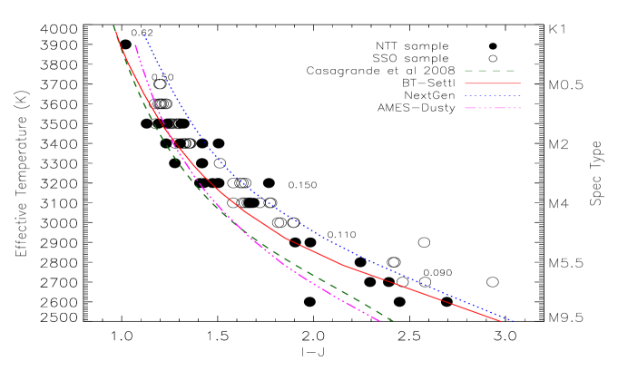
(g)

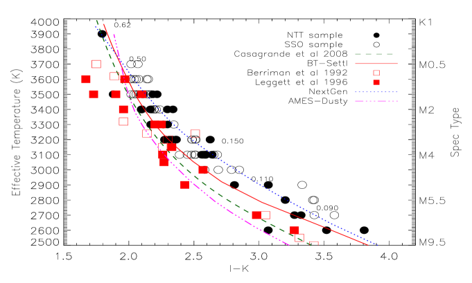
(h)

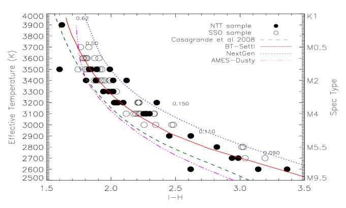
(i)

Figure 6: Continued.

$T_{\mathrm{eff}}$ versus color relations are shown in Fig. 6 in various photometric bands. The photometry of our NTT sample (filled circles) is compiled from the literature, causing a large spread particularly in the $V$ and $R$-band. The SSO 2.3 m sample (filled triangles) in comparison is more uniform. Our relations are compared to the predictions from BT-Settl isochrones at 5 Gyrs. It shows that the model is able to reproduce quite properly the colors of M-dwarfs, even in the $V$-band. There is a slight offset visible in the R-band due to missing molecular opacities (see above). These relations are compared to previously published relations when available.

Berriman et al. (1992) derive the $T_{\mathrm{eff}}$ by matching the blackbody flux anchored at $K$ band (2.2 $\mu$m) to the total bolometric flux including both the spectroscopic and photometric observed data points. They estimated the uncertainties in $T_{\mathrm{eff}}$ to be $\pm$ 4$\%$. Leggett et al. (1996) used the synthetic $I-K$ and $I-J$ colors to estimate $T_{\mathrm{eff}}$. Leggett et al. (1996) used synthetic broadband colors from the preliminary version of AMES-Dusty model produced by Allard et al. (1994). They used the $V-K$, $I-K$, $J-H$ and $H-K$ colors assuming log$g=5.0$ and solar metallicity, and found a hotter $T_{\mathrm{eff}}$-scale (by on average of 130 K) than that of Berriman et al. (1992). More recently, Casagrande et al. (2008) used the PHOENIX Cond-GAIA model atmosphere grid (P. H. Hauschildt, unpublished) to determine the atmospheric parameters of their sample of 343 nearby M dwarfs with high-quality optical and IR photometry. These models are similar to those published by Allard et al. (2001) with the exception that they were computed by solving the radiative transfer in spherical symmetry. The authors determined the $T_{\mathrm{eff}}$ using a version of the multiple optical-infrared method (IRFM) generalized to M dwarfs, and elaborated by Blackwell & Shallis (1977) and Blackwell et al. (1979, 1980). Fig. 6 shows that the Casagrande et al. (2008) $T_{\mathrm{eff}}$-scale is systematically, and progressively with decreasing $T_{\mathrm{eff}}$, cooler than the BT-Settl isochrones. Given that a large number of stars are common with Casagrande et al. (2008) sample, we did a star-by-star comparison of the $T_{\mathrm{eff}}$ determination. The values are given in Table 1 and 2. It confirms the systematic offset in the temperature scale. For cooler stars with $T_{\mathrm{eff}}<3000$ K, the $T_{\mathrm{eff}}$ determinations diverge by 100 to 300 K.

This is due, among other things, to the use of the Grevesse et al. (1993) solar elemental abundances (see Allard et al. 2012 for a comparison of the different solar elemental abundance determinations and their effects on model atmospheres).

6 Conclusion

We have compared a revised version of the BT-Settl model atmospheres (Allard et al., 2012a) to the observed NTT and SSO 2.3 m spectra and colors. This new version uses the Caffau et al. (2011) solar elemental abundances, updates to the atomic and molecular line broadening and the TiO line list from (Plez, 1998, and B. Plez, private communication). This list provides a more accurate description on the TiO bands in the M dwarfs. The systematic discrepancy between the delta- and epsilon-bands found by Reiners (2005), which seriously affected the effective temperature determination, is largely alleviated by using the (Plez, 1998, and B. Plez, private communication) TiO line list although discrepancies remain for the coolest stars. The BT-Settl models reproduce the spectral energy distribution and observed colors across the M dwarfs spectral regime to an unprecedented quality, as well as the colors. The $V$ band is also well reproduced by the models. Some discrepancies remain in the strength of some and missing other molecular absorption bands in particular in the ultraviolet spectral range.

Effective temperatures were determined by using a least-square minimization routine which gives accurate temperatures within 100 K uncertainty. We compare our temperature versus color relations using multi-wavelength photometry with the predictions from BT-Settl isochrones, assuming an age of 5 Gyrs. In general, the BT-Settl isochrones are in good agreement with the observed colors, even at temperatures below 2800 K affected by dust-treatment in the BT-Settl models. We found that the Casagrande et al. (2008) $T_{\mathrm{eff}}$-scale is systematically cooler than the BT-Settl isochrones due, among other things, to the Grevesse et al. (1993) solar elemental abundances adopted in the GAIA-Cond model atmosphere grid used for that work. The Luhman et al. (2003) $T_{\mathrm{eff}}$-scale is on the contrary progressively too hot towards the bottom of the main sequence. New interior and evolution models are currently being prepared, based on the BT-Settl models.

We provide and compare temperature versus color relations in the Optical and Infrared which matches well the BT-Settl isochrones and can be further used for large photometric datasets. We determined the effective temperature scale for the M dwarfs in our samples. Our effective temperature scale extended down to the latest-type M dwarfs where the dust cloud begins to form in their atmosphere.