Strong renormalization of the electronic band gap due to lattice polarization in the $GW$ formalism

Abstract

The self-consistent $GW$ band gaps are known to be significantly overestimated. We show that this overestimation is, to a large extent, due to the neglect of the contribution of the lattice polarization to the screening of the electron-electron interaction. To solve this problem, we derive within the $GW$ formalism a generalized plasmon-pole model that accounts for lattice polarization. The resulting $GW$ self-energy is used to calculate the band structures of a set of binary semiconductors and insulators. The lattice contribution always decreases the band gap. The shrinkage increases with the size of the longitudinal-transverse optical splitting and it can represent more than 15% of the band gap in highly polar compounds, reducing the band-gap percentage error by a factor of three.

For the past decades we have witnessed a steady increase of the accuracy of first principles electronic band structure calculations. At the lowest level we have density functional theory (DFT), normally with a local-density (LDA) or a generalized-gradient approximation (GGA) to the exchange-correlation functional. Unfortunately, the Kohn-Sham calculations strongly underestimates quasi-particle band gaps, often by more than a factor of two. At the next step, we have the $GW$ approximation of many-body perturbation theory Hedin1965 ; Hybertsen1986 ; Onida2002 . For many years, the standard practice was to start from a DFT calculation, and to evaluate perturbatively the $GW$ energy corrections to the Kohn-Sham band structure. This procedure, which we will refer to as $GW$@LDA, is justified only when the departure wave functions and band structure are already close to the quasi-particle ones. It yields a very good agreement with experimental photoemission data, especially for standard $sp$ materials. However, it is well known that $GW$@LDA fails for many crystals that have $d$ electrons participating in the states close to the band gap Bruneval2006 ; Gatti2007 ; Vidal2010 ; Vidal2010b . To solve this problem one can perform restricted self-consistent (sc) $GW$, using for example the quasi-particle (QP) sc$GW$ Faleev2004 ; Schilf2006 method or perturbative $GW$ on top of sc Coulomb hole plus screened exchange Bruneval2006 ; Bruneval2006-b ; Gatti2007 ; Vidal2010 ; Vidal2010b . The sc$GW$ techniques have the advantage of being independent of the starting point and of giving accurate results for systems that are not treatable using standard approximations, at the price of a larger computational cost. We should emphasize that these techniques allow for a precise treatment of materials that were considered out-of-reach for ab initio calculations only 10 years ago.

Unfortunately, self-consistent $GW$ calculations give too large band gaps, especially for polar materials, the simplest example being probably LiF Vidal2010 . The overestimation of the band gap within QPsc$GW$ was also discussed in literature for III-V compoundsSvane2010 , Zn-IV-N₂ Punya2011 , and transition metal oxides TiO2 ; Schilf2006 ; Vidal2010 . The causes for these errors were attributed to the lack of vertex corrections Punya2011 or to the underscreening by the random-phase approximation Svane2010 (RPA), and in both cases a simple empirical correction was adopted to improve the theoretical calculations (such as scaling the final self-energy $\Sigma_{\textrm{xc}}$ by about 80%, obtaining the so-called $0.8\Sigma$ approximation Punya2011 ).

The study of electronic correlation and its effects on the band-structure of solids has a very long tradition. A much less studied subject is, instead, the influence of phonons on the quasi-particle spectrum. Only now, in fact, the high level of accuracy achieved by electronic structure calculations makes the phonon contributions larger than the theoretical precision.

There exist two contributions to the band gap coming from phonons: i) The electron-phonon coupling, that can be handled according to the Allen-Heine-Cardona theory Allen1976 using second-order perturbation theory within the harmonic and adiabatic approximations. One obtains two terms of the same order to be included in the $GW$ self-energy, known as the Fan and Debye-Waller terms. ii) The phonon contribution to the frequency-dependent dielectric function, that can be a sizable component of the total electron screening in polar compounds.

The electron-phonon coupling terms are responsible for the strong reduction of the band gap of diamond. In fact, in that case the zero-point contribution to the band gap was proved by Giustino et al. Giustino2010 to be 0.6 eV. They observed that the example of diamond is an extreme case, while for most semiconductors and insulators the zero-point renormalization is as small as 10–50 meV Giustino2010 and can be safely neglected. The Fan and Debey-Waller terms have also been used to determine the temperature dependence of the band gap of semiconductors Liu2012 .

In this work we want to focus on the second, usually overlooked, contribution of phononic nature: the screening due to the coupling of the electro-magnetic field and the oscillating dipoles Bechstedt2005 ; Trani2010 . Of course, this contribution exists in polar materials only (and thus it is nonexistent in diamond). We should emphasize that by “polar” we mean any material that has non-negligible Born effective charges, leading to a measurable longitudinal-optical (LO) and transverse-optical (TO) phonon splitting. Most semiconducting and insulating materials known actually fit into this category. Indeed, polar materials are characterized by LO and TO infrared-active phonons, whose excitation induces macroscopic electric fields in the crystal Grosso2000 . These fields contribute, together with the electronic screening, to the total screening of the Coulomb potential, and their strength is proportional to the bond ionicity.

Already in 2005 Bechstedt et al. Bechstedt2005 observed that the lattice polarization affects significantly the dressing of the quasi-particles in ionic materials, inducing large corrections to the band gap, that they calculated using a model electronic dielectric function and a static approximation for the lattice contribution to the screening. Unfortunately, it was already observed in Ref. Bechstedt2005, that that model always overestimates the band-gap correction. In this Letter, we take a step further and develop a fully ab initio framework to include the lattice contributions to the screening within the $GW$ scheme. The basic ingredients are, besides the standard RPA screening of $GW$, the LO and TO frequencies of the infrared active phonon modes. We then calculate the electronic band structure of a set of polar materials applying this new scheme, and compare the results with experimental data and with many-body results including only electronic correlations.

The lattice polarization plays an important role in the determination of the total screening of polar compounds, as it is evident from the difference between $\epsilon_{\infty}$, the electronic dielectric function at zero frequency, and $\epsilon_{\textrm{s}}$, the total static dielectric function including contributions from both electrons and infrared active phonons. The ratio between these quantities is related to the phonon frequencies at the center of the Brillouin zone, $\omega_{\textrm{LO}}$ and $\omega_{\textrm{TO}}$, through the Lyddane-Sachs-Teller relation:

$$\frac{\omega_{\textrm{LO}}^{2}}{\omega_{\textrm{TO}}^{2}}=\frac{\epsilon_{\textrm{s}}}{\epsilon_{\infty}}\,.$$ (1)

The standard treatment of optical phonons in crystals using the dynamical matrix implicitly assumes that the interatomic interactions are instantaneous. In the case of polar crystals, the long-range nature of the Coulomb interaction requires a proper account of retardation effects. It is easy to understand that the coupling of phonon waves and electromagnetic waves is effective only for ${\bm{q}}\rightarrow{\bm{0}}$, since the speed of sound is negligible if compared with the speed of light. By combining a continuous approximation for the description of the mechanical waves of the optical modes and Maxwell’s equations for electromagnetic waves one obtains the polariton dispersion curves. For a polar crystal the total dielectric function, which includes electronic and lattice polarization terms, then reads (here for simplicity in the scalar form):

$$\epsilon({\bm{q}}\rightarrow{\bm{0}},\omega)=\epsilon_{\textrm{e}}({\bm{q}}\rightarrow{\bm{0}},\omega)+\epsilon_{\textrm{lat}}({\bm{q}}\rightarrow{\bm{0}},\omega)\,,$$ (2)

where $\epsilon_{\textrm{e}}({\bm{q}}\rightarrow{\bm{0}},\omega)$ is the long wavelength limit of the electronic contribution to the dielectric function (calculated, e.g., in the RPA approximation), and $\epsilon_{\textrm{lat}}$ is defined as the contribution to the dielectric function due to lattice polarization. This latter quantity can be related to the electronic screening by a frequency-dependent generalization of the Lyddane-Sachs-Teller relation, that reads

$$\epsilon_{\textrm{lat}}({\bm{q}}\rightarrow{\bm{0}},\omega)=\epsilon_{\textrm{e}}({\bm{q}}\rightarrow{\bm{0}},\omega)\frac{\omega_{\textrm{LO}}^{2}-\omega_{\textrm{TO}}^{2}}{\omega_{\textrm{TO}}^{2}-(\omega+{\rm i}\eta)^{2}}\,,$$ (3)

In this last expression, the infinitesimal $\eta\rightarrow 0^{+}$.

In the following discussion, and to keep the notation of the equations at a reasonably simple level, we will consider only cubic crystals with two atoms in the unit cell. However, all the equations can be easily generalized to arbitrary unit cells with more than two atoms, i.e. more than one infrared active mode Gonze-Lee .

Equations (2) and (3) can be used directly within the $GW$ framework without any further approximation. However, the very large difference between typical phonon (of the order of the meV) and electronic (of the order of the eV) frequencies makes the use of methods like the contour deformation Lebegue2003 unpractical. We will therefore resort to the popular plasmon-pole model Hybertsen1986 ; Godby1989 of the $GW$ theory in order to derive a practical framework to include the effects of lattice polarization.

For convenience, we now move to the reciprocal lattice ${\bm{G}}$ space and write $\epsilon$ as a ${\bm{G}}$, ${\bm{G}}^{\prime}$ matrix. The electronic plasmon-pole model for $\epsilon_{\textrm{e}\>{\bm{G}}{\bm{G}}^{\prime}}^{-1}(\omega,{\bm{q}})$ reads:

$$\epsilon^{-1}_{\textrm{e}\>{\bm{G}}{\bm{G}}^{\prime}}({\bm{q}},\omega)=\delta_{{\bm{G}}{\bm{G}}^{\prime}}+\frac{\Omega^{2}_{{\bm{G}}{\bm{G}}^{\prime}}({\bm{q}})}{\omega^{2}-\left[\tilde{\omega}_{{\bm{G}}{\bm{G}}^{\prime}}({\bm{q}})-{\rm i}\eta\right]^{2}}\,.$$ (4)

The two parameters $\Omega^{2}_{{\bm{G}}{\bm{G}}^{\prime}}({\bm{q}})$ and $\tilde{\omega}_{{\bm{G}}{\bm{G}}^{\prime}}({\bm{q}})$ can be fixed for example by calculating $\epsilon_{\textrm{e}\>{\bm{G}}{\bm{G}}^{\prime}}^{-1}({\bm{q}},\omega)$ at $\omega=0$ and $\omega={\rm i}\omega_{\textrm{P}}$ Godby1989 , where $\omega_{\textrm{P}}$ is the plasmon frequency. In order to determine the total screening, in the case of ${\bm{q}}\rightarrow{\bm{0}}$, one has to evaluate $\epsilon^{-1}_{{\bm{G}},{\bm{G}}^{\prime}}({\bm{q}}\rightarrow{\bm{0}},\omega)$ by inverting the sum of the two matrices $\epsilon_{\textrm{e}}({\bm{q}}\rightarrow{\bm{0}},\omega)+\epsilon_{\textrm{lat}}({\bm{q}}\rightarrow{\bm{0}},\omega)$. The way to proceed is to apply the matrix equality Miller1981

$$(G+H)^{-1}=G^{-1}-\frac{1}{1+g}G^{-1}HG^{-1}\,,$$ (5)

where

$$g=\textrm{Tr}\left\{HG^{-1}\right\}\,,$$ (6)

and $G$ is an invertible matrix. In our case the matrix $G$ is $\epsilon_{\textrm{e}\>{\bm{G}},{\bm{G}}^{\prime}}({\bm{q}}\rightarrow{\bm{0}},\omega)$ and $H$ is $\epsilon_{\textrm{lat}\>{\bm{G}},{\bm{G}}^{\prime}}({\bm{q}}\rightarrow{\bm{0}},\omega)$. A useful simplification comes from the fact that $H$ has only one non-zero element, the head of the matrix $\epsilon_{\textrm{lat}\>{\bm{0}}{\bm{0}}}({\bm{q}}\rightarrow{\bm{0}},\omega)$. In the following we will remove the explicit dependence on ${\bm{q}}$ of the dielectric matrix elements as it is clear that the lattice polarization contribution exists only for ${\bm{q}}\rightarrow{\bm{0}}$. Using (3) in (5) it is easy to show that

$$\epsilon^{-1}_{{\bm{G}}{\bm{G}}^{\prime}}(\omega)=\epsilon^{-1}_{\textrm{e}\>{\bm{G}}{\bm{G}}^{\prime}}(\omega)-\\ \frac{\epsilon^{-1}_{\textrm{e}\>{\bm{G}}{\bm{0}}}(\omega)\epsilon^{-1}_{\textrm{e}\>{\bm{0}}{\bm{G}}^{\prime}}(\omega)}{\epsilon^{-1}_{\textrm{e}\>{\bm{0}}{\bm{0}}}(\omega)}\frac{\omega^{2}_{\textrm{LO}}-\omega^{2}_{\textrm{TO}}}{\omega^{2}_{\textrm{LO}}-(\omega+{\rm i}\eta)^{2}}\,.$$ (7)

If we now replace $\epsilon^{-1}_{\textrm{e}\>{\bm{G}}{\bm{G}}^{\prime}}(\omega)$ by the standard plasmon-pole model (4) Godby1989 , we obtain our final expression for $\epsilon^{-1}_{{\bm{G}}{\bm{G}}^{\prime}}(\omega)$. The resulting formulas are quite complex, but can be simplified for the head and the wings of the inverse dielectric matrix, remembering that phonon frequencies are much smaller than the frequencies of electronic excitations. The head of the inverse dielectric matrix reads:

$$\epsilon^{-1}_{{\bm{0}}{\bm{0}}}(\omega)=1+\frac{\Omega^{2}_{{\bm{0}}{\bm{0}}}}{\omega^{2}-\left(\tilde{\omega}_{{\bm{0}}{\bm{0}}}-{\rm i}\eta\right)^{2}}-\frac{1}{\epsilon_{\infty}}\frac{\omega^{2}_{\textrm{LO}}-\omega^{2}_{\textrm{TO}}}{\omega^{2}_{\textrm{LO}}-(\omega+{\rm i}\eta)^{2}}\,,$$ (8)

where we used

$$\epsilon_{\infty}=\frac{1}{\epsilon^{-1}_{\textrm{e}\>{\bm{0}}{\bm{0}}}({\bm{q}}\rightarrow{\bm{0}},\omega_{\textrm{LO}}\approx 0)}$$ (9)

Table 1: Calculated band gaps (in eV) for the selected crystals using different $GW$ schemes compared with experimental (exp) photoemission gaps. The experimental values of $\omega_{\textrm{{LO}}}$ and $\omega_{\textrm{{TO}}}$ (in mHartree) are also given. The experimental references are given in the first column. The labels $GW^{\textrm{lat}}$ and $GW^{\textrm{lat}}$@LDA are abbreviations for sc$GW^{\textrm{lat}}$ and $GW^{\textrm{lat}}$@QPsc$GW$, respectively. The last two rows represent the mean absolute error (MAE) and mean absolute percentage error (MAPE).

	$\omega_{\textrm{{LO}}}$	$\omega_{\textrm{{TO}}}$	$GW$@LDA	$GW^{\textrm{lat}}$	QPsc$GW$	sc$GW^{\textrm{lat}}$	exp
LiF exp-LiF	2.99	1.39	13.24	12.05	15.81	13.69	14.20
LiCl exp-LiCl	1.74	0.87	8.60	7.97	10.28	9.05	9.4
NaCl exp-NaCl	1.21	0.75	7.73	7.14	9.52	8.37	8.5
MgO exp-MgO	3.29	1.82	6.97	6.38	8.94	7.71	7.7
AlP exp-AlP	2.28	2.01	2.32	2.26	2.79	2.70	2.49
AlAs exp-AlAs-GaAs	1.84	1.65	1.88	1.83	2.34	2.26	2.23
GaAs exp-AlAs-GaAs	1.30	1.22	1.16	1.15	1.52	1.46	1.52
MAE			0.60	1.04	0.74	0.18
MAPE			11.5%	16.3%	9.4%	3.0%

The matrix elements of the wings have very similar expressions, thanks to the simplification of $\epsilon^{-1}_{\textrm{e}\>{\bm{0}}{\bm{0}}}(\omega)$ appearing at the denominator in (7):

$$\epsilon^{-1}_{{\bm{G}}{\bm{0}}}=\frac{\Omega^{2}_{{\bm{G}}{\bm{0}}}}{\omega^{2}-\left(\tilde{\omega}_{{\bm{G}}{\bm{0}}}-{\rm i}\eta\right)^{2}}-\epsilon^{-1}_{\textrm{e}\>{\bm{G}}{\bm{0}}}(\omega_{\textrm{LO}})\frac{\omega^{2}_{\textrm{LO}}-\omega^{2}_{\textrm{TO}}}{\omega^{2}_{\textrm{LO}}-(\omega+{\rm i}\eta)^{2}}\,,$$ (10)

with an analogous expression for the ${\bm{0}}{\bm{G}}$ terms.

The other matrix elements of $\epsilon^{-1}_{{\bm{G}}{\bm{G}}^{\prime}}(\omega)$ are more complicated: beside the extra poles at $\omega=\pm\omega_{\textrm{LO}}$, there appear terms involving poles at $\omega=\pm\tilde{\omega}_{{\bm{G}}{\bm{0}}}$, $\omega=\pm\tilde{\omega}_{{\bm{0}}{\bm{G}}}$, and $\omega=\pm\tilde{\omega}_{{\bm{0}}{\bm{0}}}/\epsilon_{\infty}$.

We can then insert (4) and (7) in the expression for the screened Coulomb interaction $W=\epsilon^{-1}v$, where $v$ is the bare Coulomb interaction. This allows to evaluate analytically the convolution integral of the self-energy $\Sigma={\rm i}GW$

$$\Sigma({\bm{q}},\omega)=\frac{{\rm i}}{2\pi}\int_{-\infty}^{\infty}d\omega^{\prime}e^{i\eta\omega^{\prime}}G({\bm{q}},\omega+\omega^{\prime})W({\bm{q}},\omega^{\prime})\,,$$ (11)

remembering that

$$G({\bm{r}},{\bm{r}}^{\prime},\omega)=\sum_{{\bf k},j}\frac{\phi_{{\bm{k}},j}({\bm{r}})\phi^{*}_{{\bm{k}},j}({\bm{r}}^{\prime})}{\omega-\varepsilon_{{\bm{k}},j}+{\rm i}\eta\,\textrm{sign}(\varepsilon_{{\bm{k}},j}-\mu)}\,,$$ (12)

where $\phi_{{\bm{k}},j}$ are Kohn-Sham or quasi-particle orbitals, $\varepsilon_{{\bm{k}},j}$ are the corresponding energies, and $\mu$ is the Fermi level.

The frequency integration (11) is performed using the residue theorem, in strict analogy with the procedure followed for the electronic screening alone, with the only difference that more than one pole is present in the generalized plasmon-pole model that we derived. Once again, the full result is rather cumbersome, but a relatively simple expression is obtained for the lattice contribution to the matrix elements of $\Sigma$ when only the head of the matrix $\epsilon^{-1}_{{\bm{G}}{\bm{G}}^{\prime}}({\bm{q}}\rightarrow{\bm{0}},\omega)$ is retained:

$$\langle\phi_{{\bm{k}}^{\prime},j}|\Sigma_{\textrm{lat}}|\phi_{{\bm{k}}^{\prime},j}\rangle=-\frac{4\pi}{V}\frac{\omega^{2}_{\textrm{LO}}-\omega^{2}_{\textrm{TO}}}{\epsilon_{\infty}}\sum_{j}\frac{\theta(\mu-\varepsilon_{{\bm{k}}^{\prime},j})}{(\omega-\varepsilon_{{\bm{k}}^{\prime},j})^{2}-(\omega_{\textrm{LO}}-{\rm i}\eta)^{2}}\lim_{q\rightarrow{\bm{0}}}\frac{\tilde{\rho}^{*}_{{\bm{k}}^{\prime},ij}({\bm{q}}\rightarrow{\bm{0}})\tilde{\rho}_{{\bm{k}}^{\prime},ij}({\bm{q}}\rightarrow{\bm{0}})}{q^{2}}\,,$$ (13)

with $V$ the volume of the unit-cell and $\tilde{\rho}_{{\bm{k}}^{\prime},ij}({\bm{q}}\rightarrow{\bm{0}})=\lim_{{\bm{q}}\rightarrow{\bm{0}}}\int_{-\infty}^{\infty}d{\bm{r}}\phi^{*}_{{{\bm{k}}^{\prime}},i}({\bm{r}})\exp^{(-{\rm i}{\bm{q}}\cdot{\bm{r}})}\phi_{{\bm{k}}^{\prime}+{\bm{q}},j}({\bm{r}})$. Note that this term only contributes to the occupied states due to the presence of the Heaviside function $\theta(\mu-\varepsilon_{{\bm{k}}^{\prime},j})$.

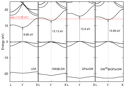
Figure 1: (Color online.) Band structure of LiF along the highest symmetry lines of the Brillouin zone. From left to right: Kohn-Sham LDA bands, $GW$@LDA bands, “standard” QPsc$GW$ bands, and $GW^{\textrm{lat}}$@QPsc$GW$ bands, including lattice polarization in the screening. The direct band gap value is also given. The experimental gap is indicated with a horizontal red line.

We implemented in abinit abinit the complete contribution of the lattice polarization to $\Sigma$, i.e., the contribution of the head, wings and body of the dielectric matrix. However, only the poles at $\omega=\pm\omega_{\textrm{LO}}$ can contribute significantly to the integral, as the coefficient in front of the other poles is always extremely small. For all systems that we studied, the contribution of the head of the matrix alone is enough to describe the correction to the band structures within less than 1 meV, but this may not be the case for non-cubic systems.

Our calculations start by the determination of the standard Kohn-Sham ground-state, using the LDA and norm-conserving pseudopotentials. The LDA Kohn-Sham states are then used to calculate $GW$@LDA band structures and as a starting point for QPsc$GW$ runs Faleev2004 . There are many different versions of $GW$, and consequently there are many different ways of using $\Sigma_{\textrm{lat}}$ in the context of $GW$. We chose as starting point a converged QPscGW calculation, as this is in our opinion the most accurate level of theory available in abinit. However, one can not use $\Sigma_{\textrm{lat}}$ in a self-consistent scheme, as this would induce contributions of the lattice polarization in $\epsilon_{\textrm{e}}$, in disagreement with Eq. (2). We therefore decided to apply the corrections due to the phonons in a final perturbative step, in what we call the $GW^{\textrm{lat}}$@QPsc$GW$ method.

In the following, we present calculations for the band structures of a set of binary compounds: LiF, LiCl, NaCl, MgO, AlP, AlAs, GaAs. These are all polar $sp$ materials, for which perturbative $GW$ gives already good band gaps, with varied bond ionicities, and band gaps ranging from 1.52 eV to 14.2 eV. All calculations were performed with abinit abinit . The energy cutoff was set to 50 Ha for LiF, LiCl, NaCl, and MgO, and to 30 Ha for the remaining compounds, and the ${\bm{k}}$-point grids were a $6\times 6\times 6$ Monkhorst-Pack. This allowed for a convergence in the total energy to better than 1 mHartree. The cutoff for the dielectric constant was set to 5 Hartree, and 142 empty states were used to obtain a convergence in the energy gaps to better than 0.1 eV. Finally, and in order to limit the effect of other possible sources of imprecision, we decided to use for these calculations experimental lattice constants and experimental LO and TO phonon frequencies at $\Gamma$ (see Table 1). Of course the method can be easily made fully ab initio by calculating such quantities within DFT abinit .

In Table 1 we report the calculated band gaps for the selected binary compounds using the different $GW$ schemes. As it is well known, $GW$@LDA underestimates the band gaps of $sp$ compounds by slightly more than 10% while QPsc$GW$ overestimates them by about 10% Schilf2006 . Turning on the correction due to lattice polarization cuts down the error of these techniques by a factor of three, bringing the mean absolute percentage error to 3%. These results clearly prove that the overestimation of the band gap by QPsc$GW$ is not mainly due to a deficient treatment of electronic correlation, but to a deficient description of the screening of the medium. We remark that the inclusion of the lattice contribution to the screening in a $GW$@LDA calculation deteriorates the agreement with experiments, leading to a mean absolute percentage error of 16%. This shows that the good performance of perturbative $GW$ calculations for $sp$ polar materials is due to a partial cancellation of errors: the underestimation of the band gap opening is compensated by the neglect of the band gap shrinkage due to the lattice polarization.

In Fig. 1 we display the band structures of LiF obtained with the different approximations under study. We can observe that the inclusion of the lattice polarization in the screening produces a rigid shift downwards of the conduction bands, with negligible effects on the band widths and band dispersions. While the same qualitative behavior is observed for all the materials under study here, we cannot exclude that other effects may be present in more complex materials.

Finally, we would like to make two remarks: (i) The coupling between electrons and phonons in our model is indirect and comes through Maxwell equations. It is therefore completely unrelated to electron-phonon coupling. (ii) To take into account all phonon contributions to the electronic band structure, both the lattice contribution to the screening and the Fan and Debye-Waller (and possibly higher order) terms of the Allen-Heine-Cardona theory Allen1976 should be included. It is true that for the materials studied here one does not expect a large contribution from the electron-phonon coupling, but it is not inconceivable to find a strong ionic compound with strong electron-phonon coupling. Note that both contributions will tend to decrease the purely electronic gap.

In conclusion, we developed a fully ab initio $GW$ framework that includes the effects of the screening owing to the polarization of the lattice. Within this framework we show that the overestimation of the band gaps by restricted self-consistent $GW$ techniques is due to the neglect of this contribution, and we manage to bring the error in the calculated band gaps to a mere 3%. The lattice contribution decreases the band gap by a factor that increases with the size of the longitudinal-transverse optical splitting and it can represent more than 15% of the band gap in highly polar compounds. These results call for a reexamination of many theoretical calculations of the quasi-particle spectrum for polar materials, including for many oxides, nitrides, etc. that are important in several fields of technology.

We would like to thank Julien Vidal and Friedhelm Bechstedt for many fruitful discussions. We acknowledge financial support from the French ANR project ANR-12-BS04-0001-02. Computational resources were provided by GENCI (project x2011096017).

References

- (1) L. Hedin, Phys. Rev. 139, A796 (1965).
- (2) M. S. Hybertsen and S. G. Louie, Phys. Rev. B 34, 5390 (1986).
- (3) G. Onida, L. Reining, and A. Rubio, Rev. Mod. Phys. 74, 601 (2002).
- (4) F. Bruneval, N. Vast, L. Reining, M. Izquierdo, F. Sirotti, and N. Barrett, Phys. Rev. Lett. 97, 267601 (2006).
- (5) M. Gatti, F. Bruneval, V. Olevano, and L. Reining, Phys. Rev. Lett. 99, 266402 (2007).
- (6) J. Vidal, S. Botti, P. Olsson, J-F. Guillemoles, and L. Reining Phys. Rev. Lett. 104, 056401 (2010).
- (7) J. Vidal, F. Trani, F. Bruneval, M.A.L. Marques, and S. Botti Phys. Rev. Lett. 104, 136401 (2010).
- (8) S.V. Faleev, M. van Schilfgaarde, and T. Kotani, Phys. Rev. Lett. 93, 126406 (2004).
- (9) M. van Schilfgaarde, T. Kotani, and S.V. Faleev, Phys. Rev. Lett. 96, 226402 (2006).
- (10) F. Bruneval, N. Vast, and L. Reining, Phys. Rev. B 74, 045102 (2006).
- (11) A. Svane, N.E. Christensen, I. Gorczyca, M. van Schilfgaarde, A.N. Chantis, and T. Kotani, Phys. Rev. B 82, 115102 (2010).
- (12) A. Punya and W.R.L. Lambrecht, and M. van Schilfgaarde, Phys. Rev. B 84, 165204 (2011).
- (13) C.E. Patrick and F. Giustino, J. Phys. Cond. Mat. 24, 202201 (2012); W. Kang and M.S. Hybertsen, Phys. Rev. B 82, 085203 (2010).
- (14) F. Giustino, S.G. Louie, and M.L. Cohen, Phys. Rev. Lett. 105, 265501 (2010).
- (15) P. B. Allen and V. Heine, J. Phys. C 9, 2305 (1976); P. Lautenschlager, P. B. Allen, and M. Cardona, Phys. Rev. B 31, 2163 (1985); Lautenschlager, P. B. Allen, and M. Cardona, Phys. Rev. B 33, 5501 (1986).
- (16) J. Liu and L. H. Liu, J. Appl. Phys. 111, 083508 (2012).
- (17) F. Bechstedt, K. Seino, P. H. Hahn, and W. G. Schmidt, Phys. Rev. B 72, 245114 (2005).
- (18) F. Trani, J. Vidal, S. Botti, and M.A.L. Marques, Phys. Rev. B 82, 085115 (2010)
- (19) G. Grosso and G. Pastori Parravicini, “Solid State Physics” (Academic Press, London, 2000).
- (20) X. Gonze and C. Lee, Phys. Rev. B 55, 10355 (1997).
- (21) S. Lebègue, B. Arnaud, M. Alouani, and P. E. Bloechl, Phys. Rev. B 67, 155208 (2003).
- (22) R. W. Godby and R. J. Needs, Phys. Rev. Lett. 62, 1169 (1989).
- (23) K. S. Miller, Mathematics Magazine 54, 67 (1981).
- (24) X. Gonze, G.-M. Rignanese, M. Verstraete, J.-M. Beuken, Y. Pouillon, R. Caracas, F. Jollet, M. Torrent, G. Zerah, M. Mikami, P. Ghosez, M. Veithen, J.-Y. Raty, V. Olevano, F. Bruneval, L. Reining, R. Godby, G. Onida, D. R. Hamann, and D. C. Allan, Z. Kristallogr. 220, 558 (2005).
- (25) G. Dollings, H. G. Smith, R.M. Nicklow, R. Vigayaraghavan, M. K. Wilkinson, Phys Rev. 168, 970 (1968); M. Piacentini, G. Lynch, and C. Olson, Phys. Rev. B 13, 5530 (1976)
- (26) M. Hass, J. of Phys. and Chem. of Solids 24, 1159 (1963); C.M. Randall, R.M. Fuller, and D.J. Montgomery, Solid State Commun. 2, 273 (1964); J.T. Lewis, A. Lehoczky, and C.V. Briscoe, Phys. Rev. 161, 877 (1967); G. Baldini and B. Bosacchi, Phys. Status Solidi 38, 325 (1970).
- (27) G. Raunio and S. Rolandson, Phys.Rev. B 2, 2098 (1970); R.T. Poole, J. Liesegang, R.C.G. Leckey, and J.G. Jenkin, Phys. Rev. B 11, 5194 (1975); R.A. Bartells and A. Smith, Phys. Rev. B 7, 3885 (1973).
- (28) R. K. Singh and K. S. Upadhyaya, Phys. Rev. B 6, 1589 (1972); A.R. Oganov, M.J. Gillan, and G.D. Price, J. Chem. Phys. 118, 10174 (2003); Ü. Özgür, Ya. I. Alivov, C. Liu, A. Teke, M. A. Reshchikov, S. Dogan, V. Avrutin, S.-J. Cho, and H. Morkoç, J. Appl. Phys. 98, 041301 (2005).
- (29) “Group IV Elements, IV-IV and III-V Compounds. Part a - Lattice Properties”, Landolt-Börnstein - Group III Condensed Matter, ed. O. Madelung, U. Rössler, M. Schulz, Vol. 41A1a, p. 1 (2001); Y.F. Tsay, A.J. Corey, and S.S. Mitra, Phys. Rev. B 12, 1354 (1975).
- (30) D. W. Palmer, www.semiconductors.co.uk, 2006.02.