Testing Quantum Gravity by Quantum Light

Abstract

In the last years quantum correlations received large attention as key ingredient in advanced quantum metrology protocols, in this letter we show that they provide even larger advantages when considering multiple-interferometer setups. In particular we demonstrate that the use of quantum correlated light beams in coupled interferometers leads to substantial advantages with respect to classical light, up to a noise-free scenario for the ideal lossless case. On the one hand, our results prompt the possibility of testing quantum gravity in experimental configurations affordable in current quantum optics laboratories and strongly improve the precision in ”larger size experiments” such as the Fermilab holometer; on the other hand, they pave the way for future applications to high precision measurements and quantum metrology

The dream of building a theory unifying general relativity and quantum mechanics, the so called quantum gravity (QG), has been a key element in theoretical physics research for the last 60 years. Several attempts in this sense have been considered. However, for many years no testable prediction emerged from these studies, leading to the common wisdom that this kind of research was more properly a part of mathematics than of physics, being by construction unable to produce experimentally testable predictions as required by Galilean scientific method. In the last few years this common wisdom was challenged am1 ; am2 ; am3 ; hog ; alt ; bek:12 . More recently, effects in interferometers connected to non-commutativity of position variables ac ; ac2 in different directions have been considered both for cavities with microresonators alt and two coupled interferometers hog , the so called “holometer”. In particular this last idea led to the planning of a double 40 m interferometer at Fermilab www.holometer .

Here we consider whether the use of quantum correlated light beams in coupled interferometers could lead to significant improvements allowing an actual simplification of the experimental apparatuses to probe the non-commutativity of position variables. On the one hand, our results demonstrate that the use of quantum correlated light can lead to substantial advantages in interferometric schemes also in the presence of non-unit quantum efficiency, up to a noise-free scenario for the ideal lossless case. This represents a big step forward respect to the quantum metrology schemes reported in literature k ; giov:11 ; Huelga:97 ; Lee:02 , and paves the way for future metrology applications. On the other hand, they prompt the possibility of testing QG in experimental configurations affordable in a traditional quantum optics laboratory with current technology.

The idea at the basis of the holometer is that non-commutativity at the Planck scale ($l_{p}=1.616\times 10^{-35}$ m) of position variables in different directions leads to an additional phase noise, referred to as holographic noise (HN). In a single interferometer ${\cal I}$ this noise substantially confounds with other sources of noise, even though the most sensible gravitational wave interferometers are considered hog , since their HN resolution is worse than their resolution to gravitational-wave at low frequencies. Nonetheless, if the two equal interferometers ${\cal I}_{1}$ and ${\cal I}_{2}$ of the holometer have overlapping spacetime volumes, then the HN between them is correlated and easier to be identified hog . Indeed, the ultimate limit for holometer sensibility, as for any classical-light based apparatus, is dictated by the shot noise: therefore, the possibility of going beyond this limit by exploiting quantum optical states is of the greatest interest giov:11 ; sch:10 ; bri:10 .

In the past the possibility of exceeding shot-noise limit in gravitational-wave detectors was suggested cav ; mc and, recently, realized ab by using squeezed light. As shown in the following, this resource can indeed allow an improvement of holometer-like apparatuses as well. Nonetheless, in this case, having two coupled interferometers, the full exploitation of properties of quantum light, and in particular of entanglement, may lead to much larger improvements.

In general, the observable measured at the output of the holometer may be described by an appropriate operator $\widehat{C}(\phi_{1},\phi_{2})$, $\phi_{k}$ being the phase shift (PS) detected by ${\cal I}_{k}$, $k=1,2$, with expectation value $\langle\widehat{C}(\phi_{1},\phi_{2})\rangle=\mathrm{Tr}[\rho_{12}\widehat{C}(\phi_{1},\phi_{2})]$, where $\rho_{12}$ is the overall density matrix associated with the state of the light beams injected in ${\cal I}_{1}$ and ${\cal I}_{2}$.

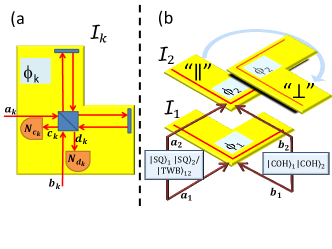
Figure 1: Sketch of the holometer. a) The two involved interferometers, ${\cal I}_{k}$, $k=1,2$, have input modes $a_{k}$ and $b_{k}$ and output modes $c_{k}\equiv c_{k}(\phi_{k})$ and $d_{k}\equiv d_{k}(\phi_{k})$, where two detectors are placed for measuring the number of photons ${\hat{N}}_{c_{k}}(\phi_{k})$ and ${\hat{N}}_{d_{k}}(\phi_{k})$, respectively. b) The interferometers are set in the configuration “$\parallel$” and “$\perp$” according to the picture. The input modes $b_{k}$, $k=1,2$, are always excited in two coherent states labeled as ”$|COH\rangle_{1}|COH\rangle_{2}$”, while the modes $a_{k}$ are excited in two uncorrelated squeezed vacua labeled as ”$|SQ\rangle_{1}|SQ\rangle_{2}$” [configuration (SQ)], or in a maximally entangled two-mode squeezed vacuum marked as ”$|TWB\rangle_{12}"$ [configuration (TWB)].

.

In order to observe the HN, one should compare hog $\langle\widehat{C}(\phi_{1},\phi_{2})\rangle$ in two different experimental configurations of ${\cal I}_{1}$ and ${\cal I}_{2}$, namely, parallel, “$\parallel$”, and perpendicular, “$\perp$” (Fig. 1). In configuration“$\parallel$”, the interferometers are oriented so that the HN induces the same random fluctuation of their PSs, leading to a substantial correlation between them, since they occupy overlapping space-time volumes hog ; footnoteA . Thus, by measuring the correlation of the interference fringes, one can highlight the presence of the HN. Configuration “$\perp$” serves as a reference measurement, namely, it corresponds to the situation where the correlation due to HN is absent, since their space-time volumes are not overlapping hog ; footnoteA , in other words, it is equivalent to the estimation of the “background”. The statistical properties of the PSs fluctuations due to HN may be described by a suitable probability density function, $f_{x}(\phi_{1},\phi_{2})$, $x=\parallel,\perp$. In turn, the expectation of any operator $\widehat{O}(\phi_{1},\phi_{2})$, or function of the PSs, should be averaged over $f_{x}$, namely,

$$\langle\widehat{O}(\phi_{1},\phi_{2})\rangle\to\mathcal{E}_{x}\left[\widehat{O}(\phi_{1},\phi_{2})\right]\equiv\int\langle\widehat{O}(\phi_{1},\phi_{2})\rangle~{}f_{x}(\phi_{1},\phi_{2})~{}\mathrm{d}\phi_{1}~{}\mathrm{d}\phi_{2}.$$ (1)

As in the holometer the HN arises as a correlation between two phases, the appropriate function to be estimated is their covariance in the parallel configuration $\mathcal{E}_{\parallel}\left[\delta\phi_{1}\delta\phi_{2}\right]$, where $\delta\phi_{k}=\phi_{k}-\phi_{k,0}$, and $\phi_{k,0}$ are the mean PS value measured by ${\cal I}_{k}$, $k=1,2$. Since the holographic noise is supposed to be small, we can expand the $\widehat{C}$ operator in terms of small fluctuation $\delta\phi_{k}$. According to Eq. (1) we are able to directly relate the covariance of the PSs to the observable quantities (see Sup. Mat. Sec. I for details):

$$\mathcal{E}_{\parallel}\left[\delta\phi_{1}\delta\phi_{2}\right]\approx\frac{\mathcal{E}_{\parallel}\left[\widehat{C}(\phi_{1},\phi_{2})\right]-\mathcal{E}_{\perp}\left[\widehat{C}(\phi_{1},\phi_{2})\right]}{\langle\partial_{\phi_{1},\phi_{2}}^{2}\widehat{C}(\phi_{1,0},\phi_{2,0})\rangle},\quad(\delta\phi_{1},\delta\phi_{2}\ll 1)$$ (2)

Eq. (2) states that the covariance can be estimated by measuring the difference between the expectation value of the operator $\widehat{C}$ in the two configurations. Thus, this difference represents the measured signal, while the coefficient at the denominator is the sensitivity.

One has to reduce as much as possible the uncertainty associated with its measurement:

$$\mathcal{U}(\delta\phi_{1}\delta\phi_{2})\approx\sqrt{\frac{\mathrm{Var}_{\parallel}\left[\widehat{C}(\phi_{1},\phi_{2})\right]+\mathrm{Var}_{\perp}\left[\widehat{C}(\phi_{1},\phi_{2})\right]}{\left[\langle\partial_{\phi_{1},\phi_{2}}^{2}\widehat{C}(\phi_{1,0},\phi_{2,0})\rangle\right]^{2}}},\quad(\delta\phi_{1},\delta\phi_{2}\ll 1)$$ (3)

where $\mathrm{Var}_{x}\left[\widehat{C}(\phi_{1},\phi_{2})\right]\equiv\mathcal{E}_{x}\left[\widehat{C}^{2}(\phi_{1},\phi_{2})\right]-\mathcal{E}_{x}\left[\widehat{C}(\phi_{1},\phi_{2})\right]^{2}$ footnote1 . We observe that the sum of variances derives from the independence of the two measurements configurations. Thanks to the same expansions leading to Eq. (2), we can write $\mathrm{Var}_{x}\left[\widehat{C}(\phi_{1},\phi_{2})\right]=\mathrm{Var}\left[\widehat{C}(\phi_{1,0},\phi_{2,0})\right]+\mathcal{O}(\delta\phi^{2})$ for both $x="\parallel","\perp"$. Therefore, the zero-order contribution to the uncertainty is

$$\mathcal{U}^{(0)}=\frac{\sqrt{2\,\mathrm{Var}\left[\widehat{C}(\phi_{1,0},\phi_{2,0})\right]}}{\left|\langle\partial_{\phi_{1},\phi_{2}}^{2}\widehat{C}(\phi_{1,0},\phi_{2,0})\rangle\right|},$$ (4)

where $\mathrm{Var}\left[\widehat{C}(\phi_{1,0},\phi_{2,0})\right]=\langle\widehat{C}(\phi_{1,0},\phi_{2,0})^{2}\rangle-\langle\widehat{C}(\phi_{1,0},\phi_{2,0})\rangle^{2}$ does not depend on the PSs fluctuations due to the HN, but it represents the intrinsic quantum fluctuations of the measurement described by the operator $\widehat{C}(\phi_{1},\phi_{2})$ and depends on the optical quantum states sent in the holometer. In particular, our aim is to look for a suitable choice of quantum optical state $\rho_{12}$ and an operator $\widehat{C}(\phi_{1},\phi_{2})$ that reduces this zero-order contribution to the uncertainty. In the following we will demonstrate that the use of quantum resources, like squeezing or, much more, entanglement, provides huge advantages in terms of achieved accuracy with respect to classical light.

As a first example we consider a configuration (SQ) where the two input modes of each interferometer ${\cal I}_{k}$, $k=1,2$, are excited in a coherent state and a squeezed vacuum state with mean number of photons $\mu_{k}$ and $\lambda_{k}$, respectively (see Fig. 1). Since the difference of the number of photons in the two output ports of each interferometer, ${\hat{N}}_{k-}(\phi_{k})={\hat{N}}_{c_{k}}(\phi_{k})-{\hat{N}}_{d_{k}}(\phi_{k})$, can be used to estimate the corresponding $\phi_{k}$ with sub-shot-noise resolution k ; giov:11 ; cav , then reasonably the covariance $\mathcal{E}_{\parallel}[\delta\phi_{1}\delta\phi_{2}]$ can be efficiently evaluated from the covariance between ${\hat{N}}_{1-}(\phi_{1})$ and ${\hat{N}}_{2-}(\phi_{2})$. Therefore we define $\widehat{C}(\phi_{1},\phi_{2})=\Delta{\hat{N}}_{1-}(\phi_{1})~{}\Delta{\hat{N}}_{2-}(\phi_{2})$, with $\Delta{\hat{N}}_{k-}(\phi_{k})={\hat{N}}_{k-}(\phi_{k})-\mathcal{E}\left[{\hat{N}}_{k-}(\phi_{k})\right]$ (we note that $\mathcal{E}_{\parallel}\left[{\hat{N}}_{k-}(\phi_{k})\right]=\mathcal{E}_{\perp}\left[{\hat{N}}_{k-}(\phi_{k})\right]=\mathcal{E}\left[{\hat{N}}_{k-}(\phi_{k})\right]$, as consequence of the properties of $f_{x}(\phi_{1},\phi_{2})$, see Sup. Mat. Sec. I).

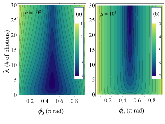
Figure 2: The uncertainty of the phase covariance $\log_{10}\mathcal{U}_{SQ}^{(0)}$ when the holometer is fed by two independent squeezed states plus two coherent fields. Here $\phi_{1,0}=\phi_{2,0}=\phi_{0}$ is the central PS of the interferometers, $\lambda_{1}=\lambda_{2}=\lambda$ is the intensity of each squeezing, $\mu_{1}=\mu_{2}=\mu$ is the intensity of each coherent beam, and their phase difference is set to zero. (a) $\mu\sim\lambda$: when the coherent and squeezed beams have similar intensities the noise reduction is lower bounded. (b) $\mu\gg\lambda$: in this regime quantum noise reduction increases with the amount of squeezing, offering a strong noise suppression if high level of squeezing can be reached. The region of the minimum runs at $\phi_{0}=\pi/2$.

Fig. 2 shows the corresponding uncertainty at the zero-order given in Eq. (4): assuming identical input states ($\mu_{k}=\mu$ and $\lambda_{k}=\lambda$, $k=1,2$), the minimum is achieved for $\phi_{1,0}=\phi_{2,0}=\pi/2$, and reads (see Sup. Mat. Sec. II):

$$\mathcal{U}_{\rm SQ}^{(0)}(\mu,\lambda)\approx\sqrt{2}~{}\frac{\lambda+\mu\left(1+2\lambda-2\sqrt{\lambda+\lambda^{2}}\right)}{(\lambda-\mu)^{2}}.$$ (5)

In perfect analogy with the PS measurement for a single interferometer cav ; mc , if $\mu\gg\lambda\gg 1$, then we have the optimal accuracy $\mathcal{U}_{\rm SQ}^{(0)}\approx(2\sqrt{2}\lambda\mu)^{-1}$. This represents a strong advantage in terms of uncertainty reduction [of the order $(4\lambda)^{-1}$] with respect to classical case $\mathcal{U}_{\rm CL}^{(0)}\approx\sqrt{2}/\mu$, i.e. when only coherent states are employed. Nevertheless, an important difference between the single interferometer PS measurement, involving a first order moment of the photon number distribution, and the covariance estimation, involving the second order momenta, arises: while in the first case the uncertainty scales as the usual standard quantum limit one, $\propto\mu^{-1/2}$, in the second case it scales $\propto\mu^{-1}$ (neglecting the little relative contribution of the squeezing to the intensity). We remark that the advantage of the present scheme is based on the independent improvement of the resolution of each interferometer which is itself limited by the amount of squeezing (see Sup. Mat. Sec. II). However, the aim of the holometer is to couple ${\cal I}_{1}$ and ${\cal I}_{2}$ minimizing the noise on their outputs correlation, namely regardless of the noise in the single interferometer. This suggests that quantum correlated states, coupling ${\cal I}_{1}$ and ${\cal I}_{2}$, could further enhance the performance of the holometer.

To this aim, we consider a new configuration (TWB) where modes $a_{1}$ and $a_{2}$ of Fig.1 are excited in a continuous variable maximally entangled state, i.e. a two-mode squeezed vacuum state or twin-beam state, $|{\rm TWB}\rangle\rangle_{a_{1},a_{2}}=S_{12}(\zeta)|0\rangle_{a_{1},a_{2}}=\sum_{n=0}^{\infty}c_{n}(\zeta)|n\rangle_{a_{1}}|n\rangle_{a_{2}}$, where $S_{12}(\zeta)=\exp(\zeta~{}a_{1}^{\dagger}a_{2}^{\dagger}-\zeta^{*}~{}a_{1}a_{2})$ is the two-mode squeezing operator. This state can be easily produced experimentally, for example by the parametric-down conversion process MandelWolf . If we set $\zeta=|\zeta|e^{i\theta_{\zeta}}$ and introduce the mean photon number per mode $\lambda=\sinh^{2}|\zeta|$, then $c_{n}(\zeta)=(1+\lambda)^{-1/2}\left[(1+\lambda^{-1})~{}e^{-i2\theta_{\zeta}}\right]^{-n/2}$ oli:12 . The input modes $b_{1}$ and $b_{2}$ are still excited in two coherent states, so that the four-mode input state is $|\psi\rangle=|{\rm TWB}\rangle\rangle_{a_{1},a_{2}}\otimes|\alpha\rangle_{b_{1}}\otimes|\alpha\rangle_{b_{2}}$.

One of the peculiarity of the state $|{\rm TWB}\rangle\rangle_{a_{1},a_{2}}$ is the presence of the same number of photons in the two modes bri:10 ; pra ; mas ; m , then each power of the photon number difference of the two modes is identically null, ${}_{a_{1},a_{2}}\langle\langle{\rm TWB}|(\hat{N}_{a_{1}}-\hat{N}_{a_{2}})^{M}|{\rm TWB}\rangle\rangle_{a_{1},a_{2}}=0$, $\forall M>0$.

We also observe that, in the absence of the HN and choosing the optimal working regime $\phi_{k,0}=0$, $k=1,2$, ${\cal I}_{1}$ and ${\cal I}_{2}$ behave like two completely transparent media for their input fields [see again Sup. Mat. Sec. II, Eq.s (4)]. In particular output modes $c_{1}$ and $c_{2}$ exhibit perfect correlation between the number of photons, which directly comes from the input modes $a_{1}$ and $a_{2}$, leading to the the natural choice of the observable as the fluctuation of the photon numbers difference, $\widehat{C}(\phi_{1},\phi_{2})=\Delta^{2}\left[{\hat{N}}_{c_{1}}-{\hat{N}}_{c_{2}}\right]$. Indeed, the numerator of Eq. (4), $\mathrm{Var}\left\{\Delta^{2}\left[{\hat{N}}_{c_{1}}(0)-{\hat{N}}_{c_{2}}(0)\right]\right\}$ is identically null, while the denominator reads:

$$\left\langle\psi\left|\partial_{\phi_{1},\phi_{2}}^{2}\Delta^{2}\left[{\hat{N}}_{c_{1}}(\phi_{1,0})-{\hat{N}}_{c_{2}}(\phi_{2,0})\right]\right|\psi\right\rangle=-\frac{1}{2}\sqrt{\lambda(1+\lambda)}\mu\cos[2(\theta_{\zeta}-\theta_{\alpha})]$$ (6)

that is non-zero for both $\lambda,\mu\neq 0$ and it is maximized for $\theta_{\zeta}-\theta_{\alpha}=0$. This quantity represents also the coefficient of proportionality in Eq. (2) between the covariance of the HN and the measured signal. It is worth noting that, even though for $\phi_{k,0}=0$ the coherent state gives no contribution to the output modes $c_{1}$ and $c_{2}$, being completely transmitted to the complementary modes $d_{1}$ and $d_{2}$, when fluctuations of the PS occurs a little portion will be reflected to the monitored ports and this guarantees the sensitivity to the HN PSs covariance.

Thus, the correlation property of the TWB state leads to the amazing result that the contribution to the uncertainty coming from the photon number noise shown in Eq. (4) is $\mathcal{U}_{\rm TWB}^{(0)}=0$ (when $\lambda,\mu\neq 0$), representing an ideal accuracy of the interferometric scheme to the PSs covariance due to HN and the main achievement of the present study.

The question that now arises is how and at which extent our conclusions are affected by a non unity overall transmission-detection efficiency $\eta$ (see Sup. Mat. Sec. III). In Fig. 3 we plot $\mathcal{U}^{(0)}$ for the SQ, TWB and classical coherent state (CL) approaches, as a function of $\eta$ (assumed to be the same for both the interferometers) for a modest level of non-classical resources ($\lambda=0.5$). As one may expect, SQ exhibits a little advantage in this regime. However, in the high efficiency region (albeit with values reasonable achievable with current technologies) the TWB-based approach provides a significant improvement not only with respect to classical set-up, but also respect to SQ.

Focusing on the limit of very small quantum resources, i.e. $\lambda\ll 1$ and $\mu\gg 1$, then $\mathcal{U}_{\rm SQ}^{(0)}/\mathcal{U}_{\rm CL}^{(0)}\approx 1-2\eta\sqrt{\lambda}$ and $\mathcal{U}_{\rm TWB}^{(0)}/\mathcal{U}_{\rm CL}^{(0)}\approx\sqrt{2(1-\eta)/\eta}$. For a small amount of squeezing the quantum noise $\mathcal{U}_{\rm SQ}^{(0)}$ not surprisingly approaches the classical case, while for TWB, we have a degradation of the performances with respect to the ideal case ($\eta=1$). Anyway, an improvement with respect to the classical case is kept for $\eta>2/3$, demonstrating that a relatively faint TWB can provide an interesting improvement in the HN detection.

In the opposite limit of high quantum resources exploited, i.e. $\mu\gg\lambda\gg 1$, $\mathcal{U}_{\rm SQ}^{(0)}/\mathcal{U}_{\rm CL}^{(0)}\approx\left(1-\eta\right)+\eta/(4\lambda)$ and $\mathcal{U}_{\rm TWB}^{(0)}/\mathcal{U}_{\rm CL}^{(0)}\approx 2\sqrt{5}\left(1-\eta\right)$ reveal that the performances of the quantum strategies are limited by the presence of the terms $(1-\eta)$. Here the main difference between SQ and TWB is that for $\eta\approx 1$ SQ exhibits an uncertainty lower bounded to $(4\lambda)^{-1}$, i.e. depending on the squeezing intensity. On the other hand, TWB approach beats the classical one for $\eta>0.683$, while for $\eta\approx 1$ it goes to zero: this demonstrates that the use of quantum light can largely improve the performances of a holometer addressed to test quantum gravity models.

A last source of noise, which could affect our results, may derive from the radiation pressure (RP) Braginsky ; cav ; Kimble . However, our model is perturbative in phase fluctuations $\delta\phi_{k}$ and, according to Eq. (5), the main noise contribution should come from the zeroth-order term corresponding to the photon noise. RP is assumed to introduce a second-order contribution to the uncertainty [see Sup. Mat. Sec. IV for details], that is related to the light fluctuation in the arms of the interferometers and to the phase shift induced by the mirrors recoil (the latter is given by $(\omega\tau/2mc)\mathcal{P}$, where $\omega$ and $\mathcal{P}$ are the central frequency of the light and the momentum of the photon, respectively, $\tau$ the measurement time and $m$ the mirrors mass cav ). In the case of a single interferometer fed by squeezed light, the amplitude of the RP noise varies with the squeezing parameter at the opposite of the photon noise, namely, if one decreases the other increases and viceversa, thus an optimum regime must be found. In the context of our proposal the behavior is similar, but for reasonable values of the involved parameters RP noise is completely negligible (justifying our perturbative approach) . Fig. 3 shows how RP noise starts to affect the uncertainty for an average coherent field intensity $\mu\gtrsim 10^{23}$ for $\tau=10^{-3}$ s (the photons introduced by the quantum modes are negligible), that is a power larger than $\hbar\omega\mu/\tau=3.3\times 10^{7}$ Watts! Since the HN must be seek in the region of the MHz, i.e. for a short measurement time ($\tau\approx 10^{-6}$ s), the RP contribution would be significant for power values larger than $10^{13}$ Watts, a value well far away from the current and future interferometry technology. One can be surprised that in the present scheme the radiation pressure is negligible, while it is not always the case for the standard phase measurement involving a single interferometer. However, we stress that here we are measuring a phase covariance between two interferometers, instead of the phase values in single ones.

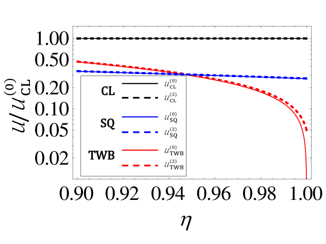
Figure 3: Uncertainty reduction normalized to the classical limit $\mathcal{U}_{CL}^{(0)}$ footnote2 . The solid lines represent the uncertainties only due to the photon noise, corresponding to the zero-order contribution [see Eq. (4)]. The coherent field intensity is set to $\mu=2\times 10^{23}$, while the twin beams and independent squeezed beams intensities are $\lambda_{1}=\lambda_{2}=\lambda=0.5$. The dashed lines represent the second-order uncertainties including the RP contribution. For its calculation the measurement time is chosen $\tau=10^{-3}$ s, the mirror mass $m=10^{2}$ Kg, and the central angular frequency of the light $\omega=3.14\times 10^{15}$ Hz (a wavelength of 600 nm.)

In conclusion, besides our analysis concerning the use of two independent squeezed states, which substantially confirms the advantages already demonstrated for gravity waves detection, the investigation carried out exploiting entanglement leads to the unprecedented result that, in an ideal situation, the background noise can be completely washed out. This achievement not only paves the way for reaching much higher sensibility in the holometer in construction at Fermilab or for the realisation of a table top experiment to test quantum gravity, but also sheds some first light on new unexpected opportunities offered by the use quantum states of light for a fundamental reduction of noise in interferometric schemes.

I Supplementary material

I.1 Derivation of Eq. (2) of the main text

Since the fluctuations due to the holographic noise (HN) are expected to be extremely small, we can expand $\widehat{C}(\phi_{1},\phi_{2})$ around the phase shift (PS) central values $\phi_{1,0}$, $\phi_{2,0}$, namely:

$$\widehat{C}(\phi_{1},\phi_{2}) = \widehat{C}(\phi_{1,0},\phi_{2,0})+\Sigma_{k}~{}\partial_{\phi_{k}}\widehat{C}(\phi_{1,0},\phi_{2,0})~{}\delta\phi_{k}+\frac{1}{2}\Sigma_{k}~{}\partial_{\phi_{k},\phi_{k}}^{2}\widehat{C}(\phi_{1,0},\phi_{2,0})~{}\delta\phi_{k}^{2}$$ (7)

$$+\partial_{\phi_{1},\phi_{2}}^{2}\widehat{C}(\phi_{1,0},\phi_{2,0})~{}\delta\phi_{1}\delta\phi_{2}+\mathcal{O}(\delta\phi^{3})$$

where $\delta\phi_{k}=\phi_{k}-\phi_{k,0}$, and $\partial_{\phi_{1}^{h},\phi_{2}^{k}}^{h+k}\widehat{C}(\phi_{1,0},\phi_{2,0})$ is the $(h+k)$-th order derivative of $\widehat{C}(\phi_{1},\phi_{2})$ calculated at $\phi_{k}=\phi_{k,0}$, $k,h=1,2$

In order to reveal the HN, the holometer exploits two different configurations: the one, “$\parallel$”, where HN correlates the interferometers, the other, “$\perp$ ”, where the effect of HN vanishes (Fig. (1) of the main text). The statistical properties of the PS fluctuations due to the HN may be described by the joint probability density functions $f_{\parallel}(\phi_{1},\phi_{2})$ and $f_{\perp}(\phi_{1},\phi_{2})$. We make two reasonable hypotheses about $f_{x}(\phi_{1},\phi_{2})$, $x=\parallel,\perp$. First, the marginals $\mathcal{F}^{(k)}_{x}(\phi_{k})=\int\mathrm{d}\phi_{h}f_{x}(\phi_{1},\phi_{2})$, $h,k=1,2$ with $h\neq k$, are exactly the same in the two configurations, i.e. $\mathcal{F}^{(k)}_{\parallel}(\phi_{k})=\mathcal{F}^{(k)}_{\perp}(\phi_{k})$: one cannot distinguish between the two configurations just by addressing one interferometer. Second, only in configuration “$\perp$” we can write $f_{\perp}(\phi_{1},\phi_{2})=\mathcal{F}^{(1)}_{\perp}(\phi_{1})\mathcal{F}^{(2)}_{\perp}(\phi_{2})$, i.e., there is no correlation between the PSs due to the HN. Now, the expectation of any operator $\widehat{O}(\phi_{1},\phi_{2})$ should be averaged over $f_{x}$, namely, $\langle\widehat{O}(\phi_{1},\phi_{2})\rangle\to\mathcal{E}_{x}\left[\widehat{O}(\phi_{1},\phi_{2})\right]\equiv\int\langle\widehat{O}(\phi_{1},\phi_{2})\rangle~{}f_{x}(\phi_{1},\phi_{2})~{}\mathrm{d}\phi_{1}~{}\mathrm{d}\phi_{2}$. In turn, by averaging the expectation of Eq. (7), we have:

$$\mathcal{E}_{x}\left[\widehat{C}(\phi_{1},\phi_{2})\right] = \langle\widehat{C}(\phi_{1,0},\phi_{2,0})\rangle+\frac{1}{2}\Sigma_{k}~{}\langle\partial_{\phi_{k},\phi_{k}}^{2}\widehat{C}(\phi_{1,0},\phi_{2,0})\rangle~{}\mathcal{E}_{x}\left[\delta\phi_{k}^{2}\right]$$ (8)

$$+\langle\partial_{\phi_{1},\phi_{2}}^{2}\widehat{C}(\phi_{1,0},\phi_{2,0})\rangle~{}\mathcal{E}_{x}\left[\delta\phi_{1}\delta\phi_{2}\right]+\mathcal{O}(\delta\phi^{3})$$

where we used $\mathcal{E}_{x}\left[\delta\phi_{k}\right]=0$. Then, according to the assumption on $f_{x}(\phi_{1},\phi_{2})$ we have $\mathcal{E}_{\parallel}\left[\delta\phi_{k}^{2}\right]=\mathcal{E}_{\perp}\left[\delta\phi_{k}^{2}\right]$ and $\mathcal{E}_{\perp}\left[\delta\phi_{1}\delta\phi_{2}\right]=\mathcal{E}_{\perp}\left[\delta\phi_{1}\right]\mathcal{E}_{\perp}\left[\delta\phi_{2}\right]=0$, and from Eq. (8) follows that the PS covariance may be written as in Eq. (2) of the main text, namely:

$$\mathcal{E}_{\parallel}\left[\delta\phi_{1}\delta\phi_{2}\right]\approx\frac{\mathcal{E}_{\parallel}\left[\widehat{C}(\phi_{1},\phi_{2})\right]-\mathcal{E}_{\perp}\left[\widehat{C}(\phi_{1},\phi_{2})\right]}{\langle\partial_{\phi_{1},\phi_{2}}^{2}\widehat{C}(\phi_{1,0},\phi_{2,0})\rangle},$$ (9)

that is proportional to the difference between the mean values of the operator $\widehat{C}(\phi_{1},\phi_{2})$ as measured in the two configurations “$\parallel$ and “$\perp$”.

Indeed, one has to reduce as much as possible the uncertainty associated with its measurement, which reads as:

$$\mathcal{U}(\delta\phi_{1}\delta\phi_{2})\approx\sqrt{\frac{\mathrm{Var}_{\parallel}\left[\widehat{C}(\phi_{1},\phi_{2})\right]+\mathrm{Var}_{\perp}\left[\widehat{C}(\phi_{1},\phi_{2})\right]}{\left[\langle\partial_{\phi_{1},\phi_{2}}^{2}\widehat{C}(\phi_{1,0},\phi_{2,0})\rangle\right]^{2}}},\quad(\delta\phi_{1},\delta\phi_{2}\ll 1)$$ (10)

where $\mathrm{Var}_{x}\left[\widehat{C}(\phi_{1},\phi_{2})\right]\equiv\mathcal{E}_{x}\left[\widehat{C}^{2}(\phi_{1},\phi_{2})\right]-\mathcal{E}_{x}\left[\widehat{C}(\phi_{1},\phi_{2})\right]^{2}$.

Under the same hypotheses used for deriving Eq. (9) we can calculate the variance of $\widehat{C}(\phi_{1},\phi_{2})$ as

$$\mathrm{Var}_{x}\left[\widehat{C}(\phi_{1},\phi_{2})\right]=\mathrm{Var}\left[\widehat{C}(\phi_{1,0},\phi_{2,0})\right]+\Sigma_{k}~{}A_{kk}~{}\mathcal{E}_{x}\left[\delta\phi_{k}^{2}\right]+A_{12}~{}\mathcal{E}_{x}\left[\delta\phi_{1}\delta\phi_{2}\right]+\mathcal{O}(\delta\phi^{3})$$ (11)

where:

$$A_{kk} = \langle\widehat{C}(\phi_{1,0},\phi_{2,0})\partial_{\phi_{k},\phi_{k}}^{2}\widehat{C}(\phi_{1,0},\phi_{2,0})\rangle$$

$$+ \langle[\partial_{\phi_{k}}\widehat{C}(\phi_{1,0},\phi_{2,0})]^{2}\rangle-\langle\widehat{C}(\phi_{1,0},\phi_{2,0})\rangle\langle\partial_{\phi_{k},\phi_{k}}^{2}\widehat{C}(\phi_{1,0},\phi_{2,0})\rangle$$

$$A_{12} = 2\langle\widehat{C}(\phi_{1,0},\phi_{2,0})\partial_{\phi_{1},\phi_{2}}^{2}\widehat{C}(\phi_{1,0},\phi_{2,0})\rangle$$

$$+ 2\langle\partial_{\phi_{1}}\widehat{C}(\phi_{1,0},\phi_{2,0})\partial_{\phi_{2}}\widehat{C}(\phi_{1,0},\phi_{2,0})\rangle-\langle\widehat{C}(\phi_{1,0},\phi_{2,0})\rangle\langle\partial_{\phi_{1},\phi_{2}}^{2}\widehat{C}(\phi_{1,0},\phi_{2,0})\rangle$$

Analyzing expression (11), we note the presence of a zeroth-order contribution that does not depend on the PSs intrinsic fluctuations, and represents the quantum photon noise of the measurement described by the operator $\widehat{C}(\phi_{1},\phi_{2})$ evaluated on the optical quantum states sent into the holometer. The statistical characteristics of the phase noise enter as second-order contributions in Eq. (11) from each interferometer plus a contribution coming from phase correlation between them.

This work addresses specifically the problem of reducing the photon noise below the shot noise in the measurement of the HN, therefore in the following and in the main text starting from Eq. (3), we assume the zero-order contribution being the dominant one. Of course, this means to look for the HN in a region of the noise spectrum that is shot-noise limited. Since the HN is expected up to frequencies of tens MHz, it follows that all the sources of mechanical vibration noise are suppressed. The only additional source of noise could be the radiation pressure, which is itself related to the light fluctuation in the arms of the interferometers. Nevertheless, we will demonstrate in Sec. I.4 that it is indeed negligible in our regime of interest.

I.2 Elements for deriving Eq. (5) of the main text

At first, we briefly review a basic aspect of the quantum description of optical interferometers. We consider two input modes described by the bosonic field operators $a$ and $b$ ($[a,a^{\dagger}]=1$ and $[b,b^{\dagger}]=1$), entering the two input ports of the optical interferometer, for instance a Michelson interferometer, as depicted in Fig. 4, whose main component is a 50:50 beam splitter (BS). The two modes interfere a first time at the BS, then they are reflected by two mirrors and interfere a second time at the BS after having gained an overall $\phi$ phase shift) induced by the difference between the optical paths of the two arms. We refer to the outgoing modes as $c$ and $d$, respectively (Fig. 4). The input/output relations can be written as MandelWolf :

$$\begin{array}[]{ll}c\equiv c(\phi)=\cos(\phi/2)~{}a-i\sin(\phi/2)~{}b,\\ d\equiv d(\phi)=-\cos(\phi/2)~{}b+i\sin(\phi/2)~{}a.\end{array}$$ (13)

We note that such input/output relations are equivalent to those of a BS with overall transmittance $\cos^{2}(\phi/2)$ (Fig. 4).

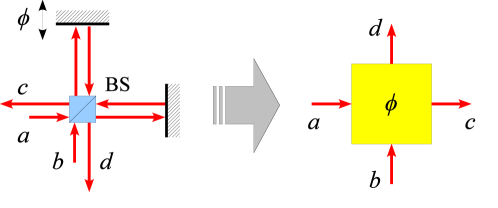
Figure 4: The action of an optical interferometer, e.g., a Michelson interferometer (left), with input modes $a$ and $b$ and output modes $c$ and $d$ measuring an overall $\phi$ phase shift between the arms can be summarized as a beam-splitter like system with transmittance $\cos^{2}(\phi/2)$ (right).

It is well known, in quantum optics community, that coherent light itself is not the optimal solution for PS estimation of an interferometer, and that the use of squeezed light may enhance the performance up to the Heisenberg limit pezze:08 . In this section we assume that the input modes $a_{k}$ and $b_{k}$ are excited in a squeezed vacuum state $|\xi_{k}\rangle_{a_{k}}=S_{a_{k}}(\xi_{k})|0\rangle_{a_{k}}$ and the coherent state $|\alpha_{k}\rangle_{b_{k}}=D_{b_{k}}(\alpha_{k})|0\rangle_{b_{k}}$, respectively, where $S_{a_{k}}(\xi_{k})=\exp[\xi_{k}~{}(a_{k}^{\dagger})^{2}-\xi_{k}^{*}~{}(a_{k})^{2}]$ is the squeezing operator and $D_{b_{k}}(\alpha_{k})=\exp(\alpha_{k}~{}b_{k}^{\dagger}-\alpha_{k}^{*}~{}b_{k})$ is the displacement operator. From now on, for the sake of simplicity, we drop the subscript $k=1,2$. If we set $\xi=|\xi|e^{i\theta_{\xi}}$ and $\alpha=\sqrt{\mu}e^{i\theta_{\alpha}}$, then $\lambda=\sinh^{2}|\xi|$ and $\mu$ represent the average number of photons of the squeezed vacuum and of the coherent state, respectively. In the case of a single interferometer, when PS is estimated from the measurement of the relative number of photons ${\hat{N}}_{-}(\phi)={\hat{N}}_{c}(\phi)-{\hat{N}}_{d}(\phi)$ [with ${\hat{N}}_{c}(\phi)=c^{\dagger}c$ and ${\hat{N}}_{d}(\phi)=d^{\dagger}d$, note that $c$ and $d$ depends on $\phi$, see Eq.s (13)], one has $\langle{\hat{N}}_{-}(\phi)\rangle=(\mu-\lambda)\cos\phi$, and in the limit $\mu\gg\lambda$, around the optimal working point $\phi=\pi/2$, the predicted uncertainty is $e^{-|\xi|}/\sqrt{\mu}$, i.e. below the shot noise or standard quantum limit caves:81 .

Following the same line of thought we investigate the possibility of exploiting the squeezed states of light also in the case of the estimation of the PSs covariance between the two interferometers. Since ${\hat{N}}_{k-}(\phi_{k})$, $k=1,2$, can be used to estimate the PS $\phi_{k}$ of the interferometer ${\cal I}_{k}$, it is reasonable to evaluate the covariance of the PSs $\mathcal{E}_{\parallel}\left[\delta\phi_{1}\delta\phi_{2}\right]$ in Eq. (9) from the covariance between ${\hat{N}}_{1-}(\phi_{1})$ and ${\hat{N}}_{2-}(\phi_{2})$. We define $\widehat{C}(\phi_{1},\phi_{2})=\Delta{\hat{N}}_{1-}(\phi_{k})~{}\Delta{\hat{N}}_{2-}(\phi_{k})$, with $\Delta{\hat{N}}_{k-}(\phi_{k})={\hat{N}}_{k-}(\phi_{k})-\mathcal{E}\left[{\hat{N}}_{k-}(\phi_{k})\right]$ and $\mathcal{E}\left[{\hat{N}}_{k-}(\phi_{k})\right]=\mathcal{E}_{\parallel}\left[{\hat{N}}_{k-}(\phi_{k})\right]=\mathcal{E}_{\perp}\left[{\hat{N}}_{k-}(\phi_{k})\right]$, according to the properties of the marginal distribution of $f_{x}(\phi_{1},\phi_{2})$. Thus, the expected value of $\widehat{C}(\phi_{1},\phi_{2})$ in each configuration is effectively the covariance between ${\hat{N}}_{1-}(\phi_{k})$ and ${\hat{N}}_{2-}(\phi_{k})$, i.e., $\mathcal{E}_{x}\left[\widehat{C}(\phi_{1},\phi_{2})\right]=\mathcal{E}_{x}\left[{\hat{N}}_{1-}(\phi_{k})~{}{\hat{N}}_{2-}(\phi_{k})\right]-\mathcal{E}\left[{\hat{N}}_{1-}(\phi_{k})\right]~{}\mathcal{E}\left[{\hat{N}}_{2-}(\phi_{k})\right]$.

We inject the state $|\psi\rangle=|\xi_{1}\rangle_{a_{1}}\otimes|\alpha_{1}\rangle_{b_{1}}\otimes|\xi_{2}\rangle_{a_{2}}\otimes|\alpha_{2}\rangle_{b_{2}}$ through $\mathcal{I}_{1}$ and $\mathcal{I}_{2}$ considering symmetry properties of the states, $\xi_{k}=\xi$, $\alpha_{k}=\alpha$ and of the interferometers $\phi_{1,0}=\phi_{2,0}=\phi_{0}$, and setting $\theta_{\alpha,1}-\theta_{\xi,1}=\theta_{\alpha,2}-\theta_{\xi,2}=0$, $k=1,2$.

According to Eq. (4) of the main text, and by substituting the input-output relations (13) into the definition of the observable $\widehat{C}(\phi_{1},\phi_{2})=\Delta{\hat{N}}_{1-}(\phi_{1})~{}\Delta{\hat{N}}_{2-}(\phi_{2})$ the minimum uncertainty becomes:

$$\mathcal{U}^{(0)}(\mu,\lambda,\phi_{0}=\pi/2)=\sqrt{2}~{}\frac{\lambda+\mu\left(1+2\lambda-2\sqrt{\lambda+\lambda^{2}}\right)}{(\lambda-\mu)^{2}}.$$ (14)

As a final comment, we remark that the advantage of the present scheme is naturally limited by the amount of squeezing. In fact, by setting $\phi=\pi/2$ in Eq.s (13), we observe that the interferometer behaves as a 50:50 BS, and the measurement of $N_{k-}$ corresponds to the quadrature measurement of the input mode $a_{k}$ by the well known homodyne detection technique, where the mode $b_{k}$ plays the role of an intense local oscillator ($\mu\gg 1$). Increasing the intensity $\lambda$ of the squeezed field in the modes $a_{k}$ means, by definition, reducing the quantum fluctuation on the measured quadrature and thus enhancing the accuracy of PS estimation in each interferometer.

I.3 The effect of losses

The overall effect of losses can be modeled by means of BSs with a suitable transmittance. Formally, this corresponds to the substitution of the output modes $c$ and $d$ of Eq.s (13) with:

$$\begin{array}[]{ll}c\to c_{\eta}=\eta^{1/2}~{}c+(1-\eta)^{1/2}~{}v_{\mathrm{c}},\\ d\to d_{\eta}=\eta^{1/2}~{}d+(1-\eta)^{1/2}~{}v_{\mathrm{d}}.\end{array}$$ (15)

that is the transmitted outputs of two identical BSs, both with transmittance $\eta$, where the modes $v_{\mathrm{c}}$ and $v_{\mathrm{d}}$ are taken in the vacuum state $|0_{v_{\mathrm{c}}}\rangle\otimes|0_{v_{\mathrm{d}}}\rangle$. Thereafter, the calculation of $\mathcal{U}_{\rm SQ}^{(0)}$ and $\mathcal{U}_{\rm TWB}^{(0)}$ as a function of $\eta$ is performed in complete analogy of the lossless case (see Sec. I.2 for independent single mode squeezed states, while for TWB see the specific paragraph of the main text).

I.4 Radiation pressure noise

Our analysis is based on the reasonable hypothesis of small phase-shift fluctuations. Therefore the main contribution to the noise should come from the intrinsic photon noise in the measurement, given by the zero-order term in Eq. (11). However, it is important to test this assumption including, at least, the effect of the other unavoidable contribution to the noise due to the radiation pressure (RP). In the context of our proposal, we demonstrate that, for reasonable values of the involved parameters, RP contribution is negligible.

The statistical properties of the RP noise are determined only by the fluctuation of the photon number inside the arms of the interferometers, that is independent of the HN. In particular, the fluctuation can be written as the sum of the two independent contributions, namely, $\delta\phi_{k}=\delta\phi_{k,HN}+\delta\phi_{k,RP}$, while the global probability density is the product of the HN density function with the RP one $F(\phi_{1,HN},\phi_{1,HN},\phi_{1,RP}\phi_{2,RP})=f_{x}(\phi_{1,HN},\phi_{2,HN})\,g(\phi_{1,RP},\phi_{2,RP})$, where we assume that $g$ is the same for $x=\parallel,\perp$. Since the variance and covariance of the PSs over $F$ are:

$$\mathcal{E}_{x}\left[\delta\phi_{k}^{2}\right] = \mathcal{E}_{x}\left[\delta\phi_{k,HN}^{2}\right]+\mathcal{E}\left[\delta\phi_{k,RP}^{2}\right],$$ (16)

$$\mathcal{E}_{x}\left[\delta\phi_{1}\delta\phi_{2}\right] = \mathcal{E}_{x}\left[\delta\phi_{1,HN}\delta\phi_{2,HN}\right]+\mathcal{E}\left[\delta\phi_{1,RP}\delta\phi_{2,RP}\right],$$ (17)

respectively, the equation (9) can be written as:

$$\mathcal{E}_{\parallel}\left[\delta\phi_{1,HN}\delta\phi_{2,HN}\right]\approx\frac{\mathcal{E}_{\parallel}\left[\widehat{C}(\phi_{1}\phi_{2})\right]-\mathcal{E}_{\perp}\left[\widehat{C}(\phi_{1},\phi_{2})\right]}{\langle\partial_{\phi_{1},\phi_{2}}^{2}\widehat{C}(\phi_{1,0},\phi_{2,0})\rangle}.$$ (18)

If the HN is absent or by far smaller than the other sources of noise, as expected, the measurement uncertainty stemming from the photon noise and the RP noise can be obtained by using Eq. (11) in the numerator of Eq. (10):

$$\mathcal{U}^{(2)}(\delta\phi_{1}\delta\phi_{2})\approx\sqrt{2\frac{\mathrm{Var}\left[\widehat{C}(\phi_{1,0},\phi_{2,0})\right]+\Sigma_{k}~{}A_{kk}~{}\mathcal{E}\left[\delta\phi_{k,RP}^{2}\right]+A_{12}~{}\mathcal{E}\left[\delta\phi_{1,RP}\delta\phi_{2,RP}\right]}{\left[\langle\partial_{\phi_{1},\phi_{2}}^{2}\widehat{C}(\phi_{1,0},\phi_{2,0})\rangle\right]^{2}}}.$$ (19)

The difference in the transferred momentum to the two mirrors of the interferometer $\mathcal{I}_{k}$ is $\mathcal{P}_{k}=(2\hbar\omega/c)\,\widehat{n}_{-,k}$, where $\widehat{n}_{-,k}$ represents the photon numbers difference in the two arms and $\omega$ is the central frequency of the light. The arms length difference induced by the RP can be written as $z_{k,RP}=(\tau/2m)\mathcal{P}_{k}$, $\tau$ being the measurement time and $m$ the masses of the mirrors, and the corresponding PS is $\phi_{k,RP}=(\omega/c)z_{k,RP}$. Therefore, the fluctuation $\delta\phi_{k,RP}$ is proportional to $\delta\widehat{n}_{-,k}=\widehat{n}_{-,k}-\langle\widehat{n}_{-,k}\rangle$ and the variance and the covariance are:

$$\mathcal{E}\left[\delta\phi_{k,RP}^{2}\right] \approx \left(\frac{\hbar\omega^{2}\tau}{c^{2}m}\right)^{2}\langle\delta\widehat{n}_{-,k}^{2}\rangle,$$ (20a)

$$\mathcal{E}\left[\delta\phi_{1,RP}\,\delta\phi_{2,RP}\right] \approx \left(\frac{\hbar\omega^{2}\tau}{c^{2}m}\right)^{2}\langle\delta\widehat{n}_{-,1}\,\delta\widehat{n}_{-,2}\rangle,$$ (20b)

respectively. The quantum expectation values in the right-hand sides of Eq.s (20) can be evaluated easily by writing $\widehat{n}_{-,k}=a^{{\dagger}}_{k,out}a_{k,out}-b^{{\dagger}}_{k,out}b_{k,out}$ according to the beam splitter input-output relations $a_{k,out}=2^{-1/2}(a_{k}+b_{k})$ and $b_{k,out}=2^{-1/2}(b_{k}-a_{k})$. In the case of independent injected squeezed states $|\psi\rangle=|\xi\rangle_{a_{1}}\otimes|\alpha\rangle_{b_{1}}\otimes|\xi\rangle_{a_{2}}\otimes|\alpha\rangle_{b_{2}}$ we have:

$$\langle\delta\widehat{n}_{-,k}^{2}\rangle_{SQ} = \lambda+\mu\left\{1+2\lambda+2\sqrt{\lambda(1+\lambda)}\cos[2(\theta_{\alpha,k}-\theta_{\xi,k})]\right\}$$ (21a)

$$\langle\delta\widehat{n}_{-,1}\,\delta\widehat{n}_{-,2}\rangle_{SQ} = 0.$$ (21b)

where we have set the optimal working point $\phi_{1,0}=\phi_{2,0}=\phi_{0}=\pi/2$. We note that here the contribution of the covariance of the photon number difference is null, because of the independence of the squeezed states sent in the two interferometers, while the variance in each interferometer agrees with the one reported in caves:81 . As in the usual treatment of a single interferometer fed by squeezed light, the amplitude of the RP noise varies with the squeezing parameter at the opposite of the photon noise (if the photon noise reduces the RP noise increases or viceversa) caves:81 .

When the expectation values in Eq.s (20) are evaluated for the TWB case, i.e. for the state $|\psi\rangle=|{\rm TWB}\rangle\rangle_{a_{1},a_{2}}\otimes|\alpha\rangle_{b_{1}}\otimes|\alpha\rangle_{b_{2}}$, we obtain:

$$\langle\delta\widehat{n}_{-,k}^{2}\rangle_{TWB} = \lambda+\mu(1+2\lambda)$$ (22a)

$$\langle\delta\widehat{n}_{-,1}\,\delta\widehat{n}_{-,2}\rangle_{TWB} = 2\mu\sqrt{\lambda(1+\lambda)}\cos[2(\theta_{\alpha,k}-\theta_{\zeta,k})].$$ (22b)

where we have set the optimal working point $\phi_{1,0}=\phi_{2,0}=\phi_{0}=0$. Comparing Eq.s (21) and Eq.s (22) one notes that the single interferometer contribution is of the same order for both “SQ” and “TWB” configurations, while the covariance of the “TWB” is non null and basically similar to the variance of the RP of the single interferometer (if $\theta_{\alpha,k}-\theta_{\zeta,k}=0$, as considered through all the paper). Even if the effect of the RP noise on the final measurement is given by Eq. (19), and requires the non trivial calculation of the coefficients $A_{kj}$, this suggests that the RP could be more effective in the case of TWB. We do not report here the lengthy calculation which leads to a cumbersome result; nevertheless, we show in Fig. 5 the behavior of the uncertainties $\mathcal{U}$ as functions of the mean number of photons of the coherent state $\mu$. It is worth noting that RP contribution is negligible for reasonable value of $\mu$, while for non-realistic higher value of $\mu$ where RP becomes relevant, TWB is a bit more penalized comparing with the case of independent squeezed states.

Summarizing, the advantage of using twin beams is not affected substantially for reasonable values of the parameters, as shown also in Fig. 3 of the main text, where the uncertainty $\mathcal{U}^{(2)}(\delta\phi_{1}\delta\phi_{2})$ of Eq. (19) is plotted as a function of the detection efficiency (see Sec. I.3).

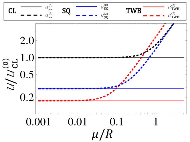
Figure 5: Uncertainty reduction normalized to the classical limit $\mathcal{U}_{CL}^{(0)}$, versus the normalized mean number of photons of the coherent fields $\mu/R$. $R=\left(\frac{\hbar\omega^{2}\tau}{c^{2}m}\right)^{-1}$ is the characteristic adimensional parameter connected with the phase-fluctuation response to the photon number fluctuation, according to Eq. (20): one has $R\approx 8.6\times 10^{24}$ for the values of $\tau,\,m$ and $\omega$ chosen in Fig. 3 of the main text. The solid lines represent the uncertainties only due to the photon noise, corresponding to the zero-order contribution [see Eq. (19)], while the dashed lines represent the second-order uncertainties including the RP noise. The twin beams and independent squeezed beams intensities are $\lambda_{1}=\lambda_{2}=\lambda=0.5$ and the overall transmission-detection efficiency $\eta=0.98$

Acknowledgements

The research leading to these results has received funding from the EU FP7 under grant agreement n. 308803 (BRISQ2), Fondazione San Paolo and MIUR (FIRB “LiCHIS” - RBFR10YQ3H and Progetto Premiale “Oltre i limiti classici di misura”), NATO grant EAP-SFPP98439.

References

(1) G. Amelino Camelia et al., ”Tests of quantum gravity from observations of gamma-ray bursts”, Nature 393, 763 (1998).
(2) G. Amelino Camelia, ”Gravity-wave interferometers as quantum-gravity detectors”, Nature 398, 216 (1999).
(3) G. Amelino Camelia, ”Astrophysics: Shedding light on the fabric of space-time”, Nature 478, 466 (2011).
(4) I. Pikovski et al., ”Probing Planck-scale physics with quantum optics”, Nature Phot. 8, 393 (2012).
(5) G. Hogan, Interferometers probes of Planckian quantum geometry, Phys. Rev. D 85, 064007 (2012).
(6) J. D. Bekenstein, ”Is a tabletop search for Planck scale signals feasible?”, arXiv:1211.3816 (2012).
(7) P.Aschieri and L. Castellani, ”Noncommutative gravity solutions”, Journ. of Geom. and Phys. 60, 375 (2010).
(8) P.Aschieri and L. Castellani, ”Noncommutative D=4 gravity coupled to fermions”, JHEP 0906, 086 (2009).
(9) Fermilab web site www.holometer.fnal.gov (03/23/2012).
(10) K. Banaszek et al., ”Quantum states made to measure”, Nature Phot. 3, 673 (2009).
(11) V. Giovannetti, S. Lloyd, and L. Maccone, ”Advances in quantum metrology”, Nature Phot. 5, 222 (2011).
(12) S. F. Huelga et al., ”Improvement of Frequency Standards with Quantum Entanglement”, Phys. Rev. Lett. 79, 3865–3868 (1997).
(13) H.Lee, P.Kook, J.Dowling, J. Mod. Opt. 49, 2325 (2002).
(14) G. Brida, M. Genovese, & I. Ruo Berchera, ”Experimental realization of sub-shot-noise quantum imaging”, Nature Phot. 4, 227 (2010).
(15) R. Schnabel, N. Mavalvala, D. E. McClelland, and P. K. Lam, ”Quantum metrology for gravitational wave astronomy”, Nature Comm. 1, 121 (2010).
(16) C. M. Caves, ”Quantum-mechanical noise in an interferometer”, Phys. Rev. D 23 , 1693 (1981).
(17) K. McKenzie et al., ”Experimental Demonstration of a Squeezing-Enhanced Power-Recycled Michelson
Interferometer for Gravitational Wave Detection”, Phys. Rev. Lett. 88 231102 (2002).
(18) Abadie et al., ”A gravitational wave observatory operating beyond the quantum shot-noise limit”, Nature Phys 7 962 (2011).
(19)The ”” configuration is relized by placing side-by-side the arms of the two interferometers, while the ”” one is implemented in the Fermilab holometer by rotating one of the interferometer of 90∘, www.holometer as sketched in Fig. 1B.
(20) An other useful interpretation of this quantity is related to the signal-to-noise ratio (SNR) of the measurement.
In general where is the signal ( for us)
that in a linear approximation is related by a certain constant ( is the denominator of Eq. (2)) to the quantity under estimation ,
in our case is the phase covariance ). The minimum resolvable value of , i.e. the one that allows to reach a SNR larger than 1, is , i.e.
exactly .
(21) L. Mandel, E. Wolf, Optical Coherence and Quantum Optics (Cambridge University Press, 1995).
(22) S. Olivares, ”Quantum optics in the phase space”, Eur. Phys. J. Special Topics 203, 3 (2012).
(23) G. Brida, M. Genovese, A. Meda, & I. Ruo Berchera, ”Experimental quantum imaging exploiting multimode spatial correlation of twin beams”, Phys. Rev. A 83, 033811
(2011).
(24) M. Bondani, A. Allevi, G. Zambra, M. G. A. Paris, & A. Andreoni, ”Sub-shot-noise photon-number correlation in a mesoscopic twin beam of light”, Phys. Rev. A 76, 013833 (2007).
(25) T. Iskhakov, M. V. Chekhova, & G. Leuchs, ”Generation and direct detection of broadband mesoscopic polarization-squeezed vacuum”, Phys. Rev. Lett. 102, 183602 (2009).
(26) Accoding to footnote1 , we have ,
thus Fig. 3 represents also the inverse of the SNRo normalized to the classical benchmark.
(27) V. B.Braginsky, F. Y. Khalili, Rev. Mod. Phys. 68, 1-11 (1996).
(28) H. J. Kimble, Y. Levin, A. B. Matsko, K. S. Thorne, S. P. Vyatchanin, Phys. Rev. D. 62, 022002 (2001).
(29) L. Mandel, E. Wolf, Optical Coherence and
Quantum Optics (Cambridge University Press, 1995).
(30) L. Pezzé and A. Smerzi, “Mach-Zehnder
interferometry at the Heisenberg limit with coherent and
squeezed-vacuum light”, Phys. Rev. Lett. 100, 073601 (2008).
(31) C. M. Caves, “Quantum mechanical noise in an
interferometer”, Phys. Rev. D 23, 1693 (1981).