Improving continuous-variable entanglement distribution by separable states

Abstract

We investigate the physical mechanism behind the counterintuitive phenomenon, the distribution of continuous-variable entanglement between two distant modes by sending a third separable auxiliary mode between them. For this purpose, we propose a new more simple and more efficient protocol resulting in distributed entanglement with more than an order of the magnitude higher logarithmic negativity than in the previously proposed protocol. This new protocol shows that the distributed entanglement originates from the entanglement of one mode and the auxiliary mode used for distribution which is first destroyed by local correlated noises and restored subsequently by the interference of the auxiliary mode with the second distant separable correlated mode.

I Introduction

Quantum entanglement is a quintessence of quantum mechanics that nowadays finds applications in the field of quantum communication and information processing. Entanglement assisted communication requires the communicating parties, Alice and Bob, to establish an entangled state between their systems $a$ and $b$. This can be done only by using a global operation, e.g. sending a quantum system $c$ between them, as entanglement cannot be created by local operations and classical communication (LOCC) Werner_89 . This, however, does not necessarily imply that the system $c$ must be entangled with the other two systems as everybody would intuitively expect. Namely, for the quantum mixed states only classical correlations and quantum interference suffice to create entanglement Cubitt_03 . Specifically, for mixed states one can establish a distillable entanglement between two qubits $a$ and $b$ by using a third qubit $c$ being always separable from the two-qubit system $(ab)$ Cubitt_03 . This phenomenon has a number of implications for quantum communication, which still have to be fully explored. For instance, quantum teleportation Bennett_93 does not require transmission of an entangled quantum system between the sender and the receiver.

Distribution of entanglement without sending entanglement was first suggested for qubits Cubitt_03 and only recently, an alternative protocol for entanglement distribution by separable states was proposed for Gaussian states of infinitely-dimensional quantum systems and quantum variables with continuous spectra-continuous variables (CVs) Mista_08 .

In this paper we study how the CV protocol works. To that aim we propose a new protocol distributing entanglement with more than an order of the magnitude higher logarithmic negativity than the previous one Mista_08 . The proposed protocol is more simple and allows to fully explain the physical mechanism underlying the phenomenon of CV entanglement distribution by separable states.

The paper is organized as follows. Section II contains a brief introduction into the formalism of Gaussian states. In Sec. III we remind the original scheme for distribution of CV entanglement by separable Gaussian states. Section IV is dedicated to the proposal of a new improved scheme for establishing entanglement using separable ancilla. In Sec. V we explain the physics behind the distribution of CV entanglement by separable states. Section VI covers conclusion and comments on the experimental feasibility of the protocol.

II Gaussian states

We consider three distinguishable infinite-dimensional quantum systems $A,B$ and $C$, referred to as “mode $A$,” “mode $B$,” and “mode $C$.” The modes are described by three pairs of canonically conjugate quadrature operators $x_{j},p_{j}$, $j=A,B,C$ satisfying the canonical commutation rules $[x_{j},x_{k}]=[p_{j},p_{k}]=0$, $[x_{j},p_{k}]=i\delta_{jk}$. Defining the column vector $\xi=(x_{A},p_{A},x_{B},p_{B},x_{C},p_{C})^{T}$ the commutation rules can be written in the compact form $[\xi_{j},\xi_{k}]=-i\Omega_{jk}$, where

$$\Omega=J\oplus J\oplus J,\quad J=\left(\begin{array}[]{cc}0&-1\\ 1&0\\ \end{array}\right)$$ (3)

is the standard three-mode symplectic matrix. All states of our three-mode system can be represented in the real six-dimensional phase space by the Wigner function Wigner_32 and Gaussian states are defined as those states for which the Wigner function is Gaussian. Any three-mode Gaussian state $\rho$ can be therefore fully characterized by the real six-dimensional vector $\langle\xi\rangle=\mbox{Tr}(\rho\xi)$ of phase-space displacements and by the $6\times 6$ real symmetric covariance matrix (CM) $\gamma$ with elements $\gamma_{jk}=\mbox{Tr}\left(\rho\{\xi_{j}-\langle\xi\rangle_{j}\openone,\xi_{k}-\langle\xi\rangle_{k}\openone\}\right)$, $j,k=1,\ldots,6$, where $\{A,B\}\equiv AB+BA$. Due to the commutation rules the CM $\gamma$ satisfies the uncertainty relation Simon_87

$$\gamma-i\Omega\geq 0.$$ (4)

In the following section we are interested in separability properties of three-mode Gaussian states and therefore we need a separability criterion for all possible $1\times 2$-mode bipartitions, i.e. bipartitions $A-(BC)$, $B-(AC)$ and $C-(AB)$. For this purpose we can use the positive partial transpose (PPT) criterion Peres_96 ; Horodecki_96 translated to Gaussian states Duan_00 ; Simon_00 ; Werner_01 ; Giedke_01 . On the level of CMs the partial transposition with respect to the mode $x$ transforms the CM $\gamma$ to $\gamma^{(T_{x})}=\Lambda_{x}\gamma\Lambda_{x}$ where $\Lambda_{x}$, $x=A,B,C$ are the diagonal matrices $\Lambda_{A}=\sigma_{z}\oplus\openone\oplus\openone$, $\Lambda_{B}=\openone\oplus\sigma_{z}\oplus\openone$, $\Lambda_{C}=\openone\oplus\openone\oplus\sigma_{z}$, where $\sigma_{z}$ is a Pauli diagonal matrix $\sigma_{z}=\mbox{diag}(1,-1)$ and $\openone$ is a $2\times 2$ identity matrix. The PPT criterion then says that a three-mode Gaussian state with CM $\gamma$ is separable with respect to bipartition $x-(yz)$ (where $(x,y,z)$ is an even permutation of $A,B,C$) if and only if the matrix $\gamma^{(T_{x})}$ satisfies the uncertainty relation (4) Giedke_01 , i.e.

$$\gamma^{(T_{x})}-i\Omega\geq 0.$$ (5)

The PPT criterion can be expressed in another equivalent form that can be sometimes easier to use in practice. It relies on the fact that for any matrix $\gamma^{(T_{x})}$ of a partially transposed state there exists a symplectic matrix $S$, i.e. a real $6\times 6$ matrix satisfying the condition $S\Omega S^{T}=\Omega$, such that $S\gamma^{(T_{x})}S^{T}=\mbox{diag}(s_{1},s_{1},s_{2},s_{2},s_{3},s_{3})$ Williamson_36 . The nonnegative quantities $s_{i}$, $i=1,2,3$ are the so called symplectic eigenvalues of $\gamma^{(T_{x})}$ and $\gamma$ is separable with respect to the splitting $x-(yz)$ if and only if $s_{i}\geq 1$ $\forall i$ Vidal_02 . The symplectic eigenvalues can be computed via the eigenvalues of the matrix $\Omega\gamma^{(T_{x})}$ which are $\left\{\pm is_{1},\pm is_{2},\pm is_{3}\right\}$. For complex three-mode states the symplectic eigenvalues are involved and it is easier to use the PPT criterion formulated in terms of the symplectic invariants Serafini_06 . The matrix $\gamma^{(T_{x})}$ possesses three such invariants denoted $I_{1},I_{2}$ and $I_{3}=\mbox{det}(\gamma^{(T_{x})})$ that can be calculated easily as coefficients of the characteristic polynomial of the matrix $\Omega\gamma^{(T_{x})}$, i.e.

$$\mbox{det}(\Omega\gamma^{(T_{x})}-\mu\openone)=\mu^{6}+I_{1}\mu^{4}+I_{2}\mu^{2}+I_{3}.$$ (6)

The criterion then says that for CM $\gamma$ mode $x$ is separable from modes $(yz)$ if and only if

$$\Sigma=\prod_{j=1}^{3}(s_{j}^{2}-1)=I_{3}-I_{2}+I_{1}-1\geq 0$$ (7)

holds. Strictly speaking, the criterion is not sufficient for separability of states having some symplectic eigenvalue equal to unity Serafini_06 . However, the sharp inequality $\Sigma>0$ is already sufficient for separability.

III The original protocol

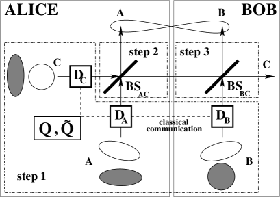
Figure 1: Two schemes of the protocol for distribution of CV entanglement by separable Gaussian states. In the original scheme Mista_08 (empty circle and ellipses) Alice’s mode $A$ and Bob’s distant mode $B$ are prepared in suitable rotated squeezed vacuum states while mode $C$ is hold by Alice and it is in a vacuum state. In the improved scheme of section IV (hatched circle and ellipses) modes $A$ and $C$ hold by Alice are in the momentum and position squeezed vacuum states, respectively, and Bob’s mode $B$ is in a vacuum state. All the three modes are then displaced by displacements $D_{A},D_{B}$ and $D_{C}$ distributed randomly with Gaussian distribution with covariance matrix $Q$ ($\tilde{Q}$ for the improved protocol) after which the modes are in a fully separable state (step 1). Mixing of modes $A$ and $C$ on a balanced beam splitter $BS_{AC}$ entangles mode $A$ with the pair of modes $(BC)$ while mode $B$ is separable from $(AC)$ and mode $C$ is separable from $(AB)$ (step 2). Mixing of modes $B$ and $C$ on a balanced beam splitter $BS_{BC}$ finally entangles $A$ and $B$ wile $C$ still remains separable from $(AB)$ (step 3). See text for details.

The original protocol for distribution of CV entanglement by separable Gaussian states Mista_08 is depicted in Fig. 1 (see figure caption for details). For this protocol the contours of the phase-space distributions of the input modes are shown as empty circle and ellipses. The essential ingredient of the protocol is a fully separable three-mode Gaussian state $\rho_{ABC}$ that transforms appropriately under beam splitter operations on certain pairs of modes. More precisely, $\rho_{ABC}$ transforms under $BS_{AC}$ operation on modes $A$ and $C$ onto a state separable with respect to two bipartitions $B-(AC)$ and $C-(AB)$ (two-mode biseparable state Giedke_01 ). This state further transforms under $BS_{BC}$ operation on modes $B$ and $C$ onto the state separable with respect to only one bipartition $C-(AB)$ (one-mode biseparable state Giedke_01 ). The construction of such a state is therefore the key nontrivial task that has to be solved in order to find the protocol. The requirements of the protocol are counterintuitive: by using LOCC and sending of a separable ancilla from Alice to Bob to create entanglement between them. As no entanglement is shared beforehand or sent by Alice to Bob, one can ask a natural question where the entanglement in the protocol comes from. In this original protocol, there is no a straightforward simple explanation for the emergence of entanglement, in particular due to the complex structure of the quantum states involved. For instance, the CMs occurring in the protocol possess correlations between position and momentum quadratures and it is fairly possible that this kind of correlations is responsible for the phenomenon. Similarly, it is not obvious which role is played by the squeezed state on Bob’s side and whether it has necessarily to be squeezed for the entanglement distribution to occur.

In the following section we show that neither of these properties accounts for the phenomenon. We construct a more simple protocol where all the participating states have zero correlations between position and momentum quadratures and where Bob’s mode is initially in the vacuum state (which is a completely classical state). Further, the new protocol exhibits a substantially better performance than the original one as it establishes entanglement between modes $A$ and $B$ with more than an order of the magnitude higher logarithmic negativity. Finally, due to its simplicity the protocol gives a clear physical explanation of the counterintuitive phenomenon of entanglement distribution by separable states.

IV The improved protocol

In contrast to the original protocol Mista_08 where the fully separable state of step 1 was constructed first, we start with designing the state in step 2. That is, by local operations on a pair of modes $(AC)$ and mode $B$ and classical communication we construct a three-mode mixed Gaussian state in which mode $A$ is entangled with modes $(BC)$, mode $C$ is separable from modes $(AB)$ and mode $B$ is separable from modes $(AC)$. Initially, we assume mode $B$ in the vacuum state and modes $A$ and $C$ in the two-mode squeezed vacuum state. The corresponding CMs read as

$$\gamma_{0,AC}=\left(\begin{array}[]{cc}\cosh(2t)\openone&\sinh(2t)\sigma_{z}\\ \sinh(2t)\sigma_{z}&\cosh(2t)\openone\\ \end{array}\right),\quad\gamma_{0,B}=\openone,$$ (10)

where $t\geq 0$ is the squeezing parameter. The matrix $\gamma_{0,AC}^{(T_{C})}$ has the lower symplectic eigenvalue equal to $\nu_{\rm in}=e^{-2t}<1$ for $t>0$ and thus modes $A$ and $C$ are entangled. Now we take the CM of the entire three-mode system,

$$\gamma_{ABC}=\left(\begin{array}[]{ccc}\cosh(2t)\openone&0&\sinh(2t)\sigma_{z}\\ 0&\openone&0\\ \sinh(2t)\sigma_{z}&0&\cosh(2t)\openone\\ \end{array}\right),$$ (14)

and we add to it a nonnegative multiple of a suitable positive noise matrix $P$ such that the state described by CM

$$\gamma_{2}=\gamma_{ABC}+xP,\qquad x\geq 0,$$ (15)

possesses entanglement between mode $A$ and modes $(BC)$ while it is separable with respect to the other two bipartitions. The matrix $P$ can be found using the method developed in Giedke_01 for construction of various three-mode entangled Gaussian states. It utilizes a two-mode version of the separability criterion represented by Eq. (5) according to which a two-mode CM $\gamma_{0,AC}$ is entangled if and only if the matrix $\gamma_{0,AC}-iJ\oplus(-J)$ has a negative eigenvalue. By adding to the CM a sufficiently large positive multiple of sum of the projectors onto the subspaces spanned by real and imaginary parts of the eigenvector corresponding to the negative eigenvalue we can destroy the entanglement between modes $A$ and $C$. Extending now the projectors suitably and adding a multiple of sum of the extensions to the CM $\gamma_{ABC}$ we can finally construct a state with desired separability properties. The negative eigenvalue is easy to find and it reads as $\lambda=-(1-e^{-2t})<0$ for $t>0$ and the corresponding eigenvector is $p_{\lambda}=p_{1}+ip_{2}$, where $p_{1}=(0,-1,0,-1)^{T}$ and $p_{2}=(1,0,-1,0)^{T}$. The sought noise matrix then can be constructed from the following $6\times 1$ extensions of the vectors $p_{1}$ and $p_{2}$:

$$q_{1} = (0,-1,0,2,0,-1)^{T},$$

$$q_{2} = (1,0,2,0,-1,0)^{T},$$ (16)

as $P=q_{1}q_{1}^{T}+q_{2}q_{2}^{T}$. The matrix is by construction positive and the addition of its sufficiently large nonnegative multiple $xP$ to the CM (14) smears the initial entanglement between modes $A$ and $C$ such that $A$ is entangled with $(BC)$ yet $C$ is separable from $(AB)$ and, furthermore, $B$ is separable from $(AC)$. The separability of mode $B$ from the pair of modes $(AC)$ is obvious as the CM (15) can be created from the product state with CM $\gamma_{0,AC}\oplus\gamma_{0,B}$ by local random correlated displacements distributed with Gaussian distribution described by the correlation matrix $xP$. The threshold value $x_{\rm sep}$ of $x$ such that for $x\geq x_{\rm sep}$ the state with CM (15) is separable with respect to $C-(AB)$ splitting can be found from the requirement of positivity of the partial transpose of the state described by CM (15) with respect to mode $C$ that is sufficient for separability of the $1\times 2$ system Werner_01 . The state has a positive partial transpose if and only if the symplectic eigenvalues $\tau_{j}$, $j=1,2,3$, of the matrix $\gamma_{2}^{(T_{C})}$ satisfy $\tau_{j}\geq 1$ for all $j$ Vidal_02 . The lowest symplectic eigenvalue reads

$$\tau_{3}=\frac{\sqrt{\left(1+6x+e^{-2t}\right)^{2}-32x^{2}}-\left(1+2x-e^{-2t}\right)}{2}$$ (17)

and the threshold value $x_{\rm sep}$ can be calculated from the condition $\tau_{3}=1$. After some algebra one can show that the CM (15) represents a state that is separable with respect to $C-(AB)$ splitting if $x\geq x_{\rm sep}$, where

$$x_{\rm sep}=\frac{e^{2t}-1}{2}.$$ (18)

Entanglement of mode $A$ with a pair of modes $(BC)$ can be verified along the same lines. The lowest symplectic eigenvalue of the matrix $\gamma_{2}^{(T_{A})}$ attains the form:

$$\omega_{3}=\frac{1+6x+e^{-2t}-\sqrt{\left(1+2x-e^{-2t}\right)^{2}+32x^{2}}}{2}$$ (19)

and for $x>0$ and $t>0$ it satisfies the inequality $\omega_{3}<1$ which proves the entanglement between $A$ and $(BC)$. Note that this entanglement is essential for the performance of the studied protocol as the second beam splitter $BS_{BC}$ alone cannot entangle mode $A$ with mode $B$ without $A$ being entangled with $(BC)$.

Having found the desired CM of step 2 we can return back to step 1 by implementing the inverse of the balanced $BS_{AC}$ on modes $A$ and $C$. The beam splitter is described by the matrix

$$U_{AC}=\left(\begin{array}[]{ccc}\frac{1}{\sqrt{2}}\openone&0&\frac{1}{\sqrt{2}}\openone\\ 0&\openone&0\\ \frac{1}{\sqrt{2}}\openone&0&-\frac{1}{\sqrt{2}}\openone\\ \end{array}\right),$$ (23)

and the inverse operation $U_{AC}^{-1}=U_{AC}^{T}=U_{AC}$ transforms the CM (15) as

$$\gamma_{1}=U_{AC}^{T}\gamma_{2}U_{AC}=\gamma_{A}\oplus\gamma_{B}\oplus\gamma_{C}+\tilde{Q},$$ (24)

where the CM $\gamma_{B}=\gamma_{0,B}=\openone$ is the vacuum CM and

$$\gamma_{A,C}=\left(\begin{array}[]{cc}e^{\pm 2t}&0\\ 0&e^{\mp 2t}\\ \end{array}\right)$$ (27)

are CMs of the momentum and position squeezed vacuum states, respectively. The structure of CM (24) reveals that the state of step 1 can be created from the product of two orthogonally squeezed states and a vacuum state by local random displacements distributed according to the Gaussian distribution with correlation matrix $\tilde{Q}=xU_{AC}^{T}PU_{AC}$ that has the following form:

$$\tilde{Q}=x\left(\begin{array}[]{ccc}\openone-\sigma_{z}&\sqrt{2}(\sigma_{z}-\openone)&0\\ \sqrt{2}(\sigma_{z}-\openone)&4\cdot\openone&\sqrt{2}(\sigma_{z}+\openone)\\ 0&\sqrt{2}(\sigma_{z}+\openone)&\sigma_{z}+\openone\\ \end{array}\right).$$ (31)

This implies immediately that the state is fully separable as is the basic requirement of our protocol.

The improved protocol for distribution of CV entanglement by separable Gaussian states is depicted in Fig. 1. The phase-space contours of the input modes for this protocol are represented by hatched circle and ellipses. As follows from the CM $\gamma_{1}$ designed in Eqs. (24) and (27), the input modes $A$ and $C$ are both in a squeezed state with reduced noise in two orthogonal quadratures respectively and mode $B$ is in a vacuum state. In the step 1 Alice holding a pair of modes $(AC)$ and Bob holding mode $B$ prepare by LOCC a Gaussian state characterized by the CM (24). In the next step 2, Alice superimposes mode $A$ and $C$ on a balanced beam splitter $BS_{AC}$. Thus she creates a state with CM (15) that reads explicitly

$$\gamma_{2}=\left(\begin{array}[]{ccc}a\openone&2x\sigma_{z}&b\sigma_{z}\\ 2x\sigma_{z}&(1+4x)\openone&-2x\openone\\ b\sigma_{z}&-2x\openone&a\openone\\ \end{array}\right),$$ (35)

where $a=\cosh(2t)+x$ and $b=\sinh(2t)-x$. As was shown above, the state is separable with respect to $B-(AC)$ splitting and for $x\geq x_{\rm sep}$, where $x_{\rm sep}$ is given in Eq. (18), also with respect to $C-(AB)$ splitting.

The protocol is finalized by step 3 in which Bob mixes the mode $C$ received from Alice with his mode $B$ on another balanced beam splitter $BS_{BC}$ described by the matrix

$$U_{BC}=\left(\begin{array}[]{ccc}\openone&0&0\\ 0&\frac{1}{\sqrt{2}}\openone&\frac{1}{\sqrt{2}}\openone\\ 0&\frac{1}{\sqrt{2}}\openone&-\frac{1}{\sqrt{2}}\openone\\ \end{array}\right).$$ (39)

The beam splitter transforms the CM (35) to CM $\gamma_{3}=U_{BC}\gamma_{2}U_{BC}^{T}$ that reads explicitly as

$$\gamma_{3}=\left(\begin{array}[]{ccc}a\openone&\frac{2x+b}{\sqrt{2}}\sigma_{z}&\frac{2x-b}{\sqrt{2}}\sigma_{z}\\ \frac{2x+b}{\sqrt{2}}\sigma_{z}&\frac{1+a}{2}\openone&\frac{1+4x-a}{2}\openone\\ \frac{2x-b}{\sqrt{2}}\sigma_{z}&\frac{1+4x-a}{2}\openone&\frac{1+8x+a}{2}\openone\\ \end{array}\right),$$ (43)

where $a$ and $b$ are defined as in Eq. (35). The interference on the beam splitter $BS_{BC}$ finally entangles modes $A$ and $B$. This can be seen by computing the lower symplectic eigenvalue $\nu$ of the matrix $\gamma_{3,AB}^{(T_{B})}$ corresponding to the reduced state of modes $A$ and $B$. We express the CM $\gamma_{3,AB}$ in the block form

$$\gamma_{3,AB}=\left(\begin{array}[]{cc}A&C\\ C^{T}&B\\ \end{array}\right),$$ (46)

where $A,B$ and $C$ are $2\times 2$ submatrices. The eigenvalue then reads as Vidal_02

$$\nu=\sqrt{\frac{\kappa-\sqrt{\kappa^{2}-4\mbox{det}(\gamma_{3,AB})}}{2}},$$ (47)

where

$$\mbox{det}\left(\gamma_{3,AB}\right) = \left[\frac{1+\cosh\left(2t\right)}{2}+\left(e^{-2t}+\frac{1}{2}\right)x\right]^{2},$$

$$\kappa = \mbox{det}A+\mbox{det}B-2\mbox{det}C$$ (48)

$$= a^{2}+\left(b+2x\right)^{2}+\frac{\left(a+1\right)^{2}}{4}$$

and it can be used to quantify the amount of distributed entanglement by calculating the logarithmic negativity given by the formula $E_{\mathcal{N}}=-\log_{2}\nu$ Vidal_02 . For $t>0$ and $x=x_{\rm sep}=(e^{2t}-1)/2$ we get $\nu<1$ and therefore modes $A$ and $B$ are entangled for an arbitrarily small nonzero squeezing. Numerical analysis further reveals that the symplectic eigenvalue decreases monotonously with increasing squeezing and approaches the value of $\nu=1/3$ corresponding to $E_{\mathcal{N}}\approx 1.585$ ebits in the limit of infinite squeezing while all the separability properties of the states involved remain preserved. To illustrate this, we have calculated the output entanglement for some realistic values of squeezing using Eqs. (47) and (IV). Thus $e^{2t}=2$ corresponding to 3dB of input squeezing results in the symplectic eigenvalue of $\nu\approx 0.6589$ which gives the logarithmic negativity of $E_{\cal N}\approx 0.6019$ ebits. For $e^{2t}=10$ corresponding to 10dB squeezing that was recently achieved experimentally Schnabel_08 we get $\nu\approx 0.3968$ and $E_{\cal N}\approx 1.3334$ ebits.

It is interesting to compare the latter logarithmic negativity with the maximum logarithmic negativity that can be obtained with the original protocol Mista_08 . Numerical optimization of the original protocol with respect to the noise parameter $x$ and the initial squeezings (denoted by $d\pm r$ in Mista_08 ) reveals that the minimal lower symplectic eigenvalue of the partially transposed final entangled state distributed between Alice and Bob reads as $\nu\approx 0.9299$ and the corresponding logarithmic negativity is $E_{\cal N}\approx 0.1048$ ebits. Thus the logarithmic negativity of the entangled state created between distant locations in the improved protocol is more than an order of the magnitude higher than in the original protocol. Furthermore, also in this improved protocol the mode $C$ remains separable from modes $(AB)$ after the step 3. This can be shown using the separability criterion based on symplectic invariants Serafini_06 . For example, for $e^{2t}=2$ the criterion gives $\Sigma=1>0$ which implies separability of mode $C$ from $(AB)$.

V Explanation of the protocol

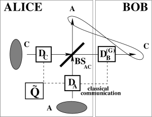
Figure 2: Scheme of the protocol for recovery of the entanglement between modes $A$ and $C$. Mode $A$ in a suitable momentum-squeezed vacuum state and mode $C$ in a position-squeezed vacuum state with the same level of squeezing are displaced by displacements $D_{A}$ and $D_{C}$ distributed randomly with Gaussian distribution characterized by the covariance matrix $\tilde{Q}$ (31). Next, the two modes are mixed on a balanced beam splitter $BS_{AC}$ that prepares them in a two-mode separable state. Classical information traveling to Bob is then used for displacement $D_{B}^{(G)}$ of mode $C$ with a suitable electronic gain $G$. Provided that the gain is adjusted appropriately, the entanglement between modes $A$ and $C$ can be perfectly recovered. See text for details.

The previous sections reveal that there indeed exist three-mode mixed Gaussian fully separable states allowing to entangle two modes of the state by mixing them stepwise with the third always separable mode on two beam splitters. Therefore, once such a tripartite state is established between distant Alice and Bob, they can create, without need of any additional knowledge, entanglement between them by sending a separable mode from one site to another remote location. There is, however, another interesting aspect in this protocol. When looking at the scheme in Fig. 1, one can imagine a different scenario when Bob has some additional information about the preparation of the shared state. Specifically, suppose that in each run of the protocol he knows classical displacements $\bar{x}_{B},\bar{p}_{B}$ used to displace his vacuum mode $B$. The natural question arises whether Alice and Bob can then create a higher entanglement than when using solely the shared fully separable state. In what follows we give an affirmative answer to this question by showing that they can in fact restore the whole amount of entanglement contained in the two-mode squeezed vacuum state with CM $\gamma_{0,AC}$ defined in Eq. (10). Moreover, here we provide an explanation where the entanglement comes from in the improved protocol depicted in Fig. 1.

Let us consider the scheme in Fig. 2. There, the situation on Alice’s side remains the same as in the protocol in Fig. 1. Bob, however, does not use an auxiliary vacuum mode $B$ appropriately displaced with $D_{\rm B}$ to achieve the desired final CM. Instead, he directly displaces mode $C$ received from Alice with a suitable electronic gain $G$. The CM of the resulting state is most easily calculated in Heisenberg picture. Let us denote by $x_{A}^{(0)}$, $p_{A}^{(0)}$, $x_{C}^{(0)}$ and $p_{C}^{(0)}$ position and momentum quadratures of initially vacuum modes $A$ and $C$, respectively. Arranging the quadratures of the squeezed vacuum modes $A$ and $C$ into the column vectors $\xi_{A}=(x_{A},p_{A})^{T}=(e^{t}x_{A}^{(0)},e^{-t}p_{A}^{(0)})^{T}$ and $\xi_{C}=(x_{C},p_{C})^{T}=(e^{-t}x_{C}^{(0)},e^{t}p_{C}^{(0)})^{T}$, the quadratures of modes $A$ and $C$ after the displacements $D_{A}$ and $D_{C}$ read $\xi_{A}+\bar{\xi}_{A}$ and $\xi_{C}+\bar{\xi}_{C}$, where the vectors $\bar{\xi}_{A}=(\bar{x}_{A},\bar{p}_{A})^{T}$ and $\bar{\xi}_{C}=(\bar{x}_{C},\bar{p}_{C})^{T}$ define classical displacements. Next, the two modes are mixed on the balanced beam splitter $BS_{AC}$. Further, mode $C$ undergoes the displacement $D_{B}^{(G)}$ defined by the displacement vector $\bar{\xi}_{B}=(\bar{x}_{B},\bar{p}_{B})^{T}$ of mode $B$ and $2\times 2$ gain matrix $G$. This yields finally the transformed quadratures in the following form:

$$\xi_{A}^{\prime\prime} = \frac{\xi_{A}+\bar{\xi}_{A}+\xi_{C}+\bar{\xi}_{C}}{\sqrt{2}},$$

$$\xi_{C}^{\prime\prime} = \xi_{C}^{\prime}+G\bar{\xi}_{B}=\frac{\xi_{A}+\bar{\xi}_{A}-\xi_{C}-\bar{\xi}_{C}}{\sqrt{2}}+G\bar{\xi}_{B}.$$

Here $\xi_{C}^{\prime}$ is the vector of quadratures of mode $C$ behind the beam splitter $BS_{AC}$. To determine the final state of a two-mode subsystem $(AC)$, one has first to calculate the correlations $A_{ij}=\langle\{\xi_{A,i}^{\prime\prime},\xi_{A,j}^{\prime\prime}\}\rangle$, $C_{ij}=\langle\{\xi_{C,i}^{\prime\prime},\xi_{C,j}^{\prime\prime}\}\rangle$ for modes $A$ and $C$, respectively, and the intermodal correlations $\Gamma_{ij}=\langle\{\xi_{A,i}^{\prime\prime},\xi_{C,j}^{\prime\prime}\}\rangle$, $i,j=1,2$, where the angle brackets denote averaging of the quantum quadrature operators over the quantum state with CM $\gamma_{A}\oplus\openone_{B}\oplus\gamma_{C}$, where $\gamma_{A,C}$ are defined in Eq. (27) and the classical displacements are averaged over the Gaussian distribution with covariance (31). Using Eqs. (V), CMs (27) and the correlation matrix (31) and taking into account the fact that the vectors of quantum quadratures $\xi_{A},\xi_{C}$ are uncorrelated with the vectors of classical displacements $\bar{\xi}_{A},\bar{\xi}_{B}$ and $\bar{\xi}_{C}$, we arrive at the CM of the state of modes $A$ and $C$

$$\gamma_{2,AC}^{(G)}=\left(\begin{array}[]{cc}A&\Gamma\\ \Gamma^{T}&C\\ \end{array}\right),$$ (52)

where

$$A = a\openone,\quad\Gamma=\sigma_{z}(b\openone+2xG^{T}),$$

$$C = a\openone+4xGG^{T}-2x(G+G^{T}),$$ (53)

where the parameters $a$ and $b$ are defined below Eq.(35). The structure of the CM indicates the optimal choice of the gain matrix $G$. We see that by choosing $G=G_{\rm opt}=\openone$ the noise in the diagonal block $C$ cancels and the CM transforms to

$$\gamma_{2,AC}^{(G_{\rm opt})}=\left(\begin{array}[]{cc}a\openone&(b+2x)\sigma_{z}\\ (b+2x)\sigma_{z}&a\openone\\ \end{array}\right).$$ (56)

To characterize the separability properties of CM $\gamma_{2,AC}^{(G_{\rm opt})}$, it remains to calculate the lower symplectic eigenvalue $\nu_{AC}$ for the matrix $\left(\gamma_{2,AC}^{(G_{\rm opt})}\right)^{(T_{C})}$. Using Eq. (47) one finds that it attains the simple form $\nu_{AC}=a-b-2x=e^{-2t}$. Hence we immediately see that the eigenvalue coincides with the lower symplectic eigenvalue $\nu_{\rm in}=e^{-2t}$ of the partially transposed pure two-mode squeezed vacuum state with CM (10) that can be prepared by Alice from her pure squeezed states. Since any Gaussian operation on mode $C$ cannot increase the entanglement of the state with CM (56) Eisert_02 we see that Bob’s displacement on mode $C$ with the gain matrix $G_{\rm opt}$ is indeed an optimal Gaussian operation. It is worth mentioning that while the entanglement of the two-mode squeezed vacuum state figuring in the protocol can be restored perfectly, the purity of the state cannot because $\mbox{det}(\gamma_{2,AC}^{(G_{\rm opt})})=\left(1+2xe^{-2t}\right)^{2}$.

Previous analysis reveals the origin of the entanglement in the improved protocol in Fig. 1. The displacements $D_{A}$ and $D_{C}$ before the beam splitter $BS_{AC}$ can be transformed to another displacements $D_{A}^{\prime}$ and $D_{C}^{\prime}$ behind the beam splitter. Consequently, the state of modes $A$ and $C$ behind the beam splitter can be viewed as a pure two-mode squeezed vacuum state with CM (10). The entanglement and purity of this state is then subsequently destroyed by local correlated displacements $D_{A}^{\prime}$ and $D_{C}^{\prime}$. The classical information on displacements $\bar{x}_{B}$ and $\bar{p}_{B}$ traveling to Bob, that as we have seen allows him to perfectly restore the entanglement between modes $A$ and $C$ if he uses the protocol of Fig. 2, is instead used to displace his vacuum mode $B$. Mixing of the displaced vacuum mode $B$ with mode $C$ on the second balanced beam splitter $BS_{BC}$ leads finally to the following vector of Bob’s quadratures:

$$\xi_{B,{\rm out}}=\frac{\xi_{C}^{\prime}+\bar{\xi}_{B}+\xi_{B}^{(0)}}{\sqrt{2}},$$ (57)

where $\xi_{B}^{(0)}=(x_{B}^{(0)},p_{B}^{(0)})^{T}$ is the vector of Bob’s vacuum quadratures and $\xi_{C}^{\prime}$ denotes the vector of quadratures of mode $C$ behind the beam splitter $BS_{AC}$. Compare the last equation with the equation for the vector of optimal quadratures $\xi_{C}^{\prime\prime}=\xi_{C}^{\prime}+\bar{\xi}_{B}$ obtained by setting $G=G_{\rm opt}=\openone$ in equation for $\xi_{C}^{\prime\prime}$ in Eqs. (V). We find out that the vector of output Bob’s quadratures (57) is obtained from the vector of optimal quadratures by mixing it with the vector of vacuum quadratures of Bob’s mode on a balanced beam splitter described by Eq. (39). Thus, mixing of mode $C$ with mode $B$ on a beam splitter $BS_{BC}$ in Fig. 1 implements effectively optimal displacement of mode $C$ restoring perfectly entanglement between modes $A$ and $C$ followed by mixing of the mode with the vacuum mode on a balanced beam splitter which reduces the amount of the entanglement. This finally explains the origin of the distributed entanglement in the improved protocol as well as the fact that it is weaker in comparison with the maximum entanglement that can be restored by Bob using the scheme in Fig. 2 with optimal gain matrix $G_{\rm opt}$.

VI Conclusion

In conclusion, we performed a detailed investigation of the origin of entanglement in the protocol for entanglement distribution by separable Gaussian states Mista_08 . For this purpose we proposed a more simple and efficient protocol that enables to distribute entanglement with more than an order of the magnitude higher logarithmic negativity than the older protocol Mista_08 . Based on the new protocol we then found that the distributed entanglement originates from the entanglement of sender’s mode with the auxiliary mode that is used for distribution. The entanglement is first destroyed by local correlated displacements that make the auxiliary mode separable from sender’s mode. The separable mode is then sent to the receiver who partially restores the entanglement by mixing it with his suitably classically correlated mode.

We emphasize that the proposed protocol for establishing entanglement between two remote parties using separable ancilla mode consists of experimentally feasible Gaussian states and operations involving single-mode squeezed states, correlated displacements and beam splitters, dispensing with the technically challenging CNOT gates of the qubit case. The input squeezed states with CMs (27) need not to be minimum uncertainty states and the protocol works well also with states with a large noise excess in the antisqueezed quadratures, e.g., for $e^{2t}=2$ and $200$ vacuum units of noise excess in each quadrature the logarithmic negativity of the distributed entanglement is $E_{\cal N}\approx 0.5851$ ebits compared to $E_{\cal N}\approx 0.6019$ ebits for the minimum uncertainty states.

The verification of the effect, however, can become an issue, as the possibility to demonstrate experimentally the proposed protocol crucially relies on our ability to check separability of mode $C$ from the pair of modes $(AB)$ in step 2. In theory we assumed Gaussianity of states involved in the protocol. This enabled us to prove the separability using relatively simple sufficient conditions for separability of Gaussian states Vidal_02 ; Serafini_06 . In an experiment, however, in order to check whether the state prepared by us is Gaussian we would have to perform complete tomography of the state on infinite-dimensional state space which amounts to infinite number of measurements. In this sense the Gaussian states are idealized limit states and for the experimental demonstration of the protocol we therefore need a sufficient condition for separability of a generic generally non-Gaussian state or a reliable indication, that the Gaussian character of the states is preserved throughout the protocol. Nevertheless, a less ambitious goal can be achieved by measuring only the three-mode CM of the state in step 2. By showing that the measured CM satisfies some Gaussian sufficient condition for separability of mode $C$ from modes $(AB)$ we know that the Gaussian entanglement of modes $A$ and $B$ was distributed by sending an ancilla that was separable in Gaussian sense.

- (1) R. F. Werner, Phys. Rev. A 40, 4277 (1989).
- (2) T. S. Cubitt, F. Verstraete, W. Dür, and J. I. Cirac, Phys. Rev. Lett. 91, 037902 (2003).
- (3) C. H. Bennett, G. Brassard, C. Crépeau, R. Jozsa, A. Peres, and W. K. Wootters, Phys. Rev. Lett. 70, 1895 (1993).
- (4) L. Mišta, Jr., and N. Korolkova, Phys. Rev. A 77, 050302(R) (2008).
- (5) E. P. Wigner, Phys. Rev. 40, 749 (1932).
- (6) R. Simon, E. C. G. Sudarshan, and N. Mukunda, Phys. Rev. A 36, 3868 (1987).
- (7) A. Peres, Phys. Rev. Lett. 77, 1413 (1996).
- (8) M. Horodecki, P. Horodecki, and R. Horodecki, Phys. Lett. A 223, 1 (1996).
- (9) L.-M. Duan, G. Giedke, J. I. Cirac, and P. Zoller, Phys. Rev. Lett. 84, 2722 (2000).
- (10) R. Simon, Phys. Rev. Lett. 84, 2726 (2000).
- (11) R. F. Werner and M. M. Wolf, Phys. Rev. Lett. 86, 3658 (2001).
- (12) G. Giedke, B. Kraus, M. Lewenstein, and J. I. Cirac, Phys. Rev. A 64, 052303 (2001).
- (13) J. Williamson, Am. J. Math. 58, 141 (1936).
- (14) G. Vidal and R. F. Werner, Phys. Rev. A 65, 032314 (2002).
- (15) A. Serafini, Phys. Rev. Lett. 96, 110402 (2006); A. Serafini, J. Opt. Soc. Am. B 24, 347 (2007).
- (16) H. Vahlbruch, M. Mehmet, S. Chelkowski, B. Hage, A. Franzen, N. Lastzka, S. Goßler, K. Danzmann, and R. Schnabel, Phys. Rev. Lett. 100, 033602 (2008).
- (17) J. Eisert, S. Scheel, and M. B. Plenio, Phys. Rev. Lett. 89, 137903 (2002); J. Fiurášek, Phys. Rev. Lett. 89, 137904 (2002); G. Giedke and J. I. Cirac, Phys. Rev. A 66, 032316 (2002).