Abstract

We analyze electrostatic potentials in the holographic Schwinger effect. The potential barrier for the pair production is estimated by a static potential consisting of static mass energies, an electric potential from an external electric-field, and the Coulomb potential between a particle and an antiparticle. Given that the Coulomb potential is supposed to be evaluated by the minimal surface attaching on the conformal boundary as usual, the critical field, where the potential barrier vanishes, exhibits a deviation of 30$\%$ from the one obtained from the Dirac-Born-Infeld (DBI) action. We reconsider this issue by reexamining the Coulomb-potential part, which is evaluated by the classical action of a string solution attaching on a probe D3-brane sitting at an intermediate position in the bulk AdS. Then the resulting critical-field completely agrees with the DBI result. This agreement gives rise to a strong support for the holographic scenario. We also discuss the finite-temperature case and the temperature-dependent critical-field also agrees with the DBI result.

1 Introduction

The Schwinger effect [1] is known as a non-perturbative phenomenon in quantum electromagnetic dynamics (QED). The virtual electron-position pairs can become real particles due to the presence of a strong electric-field. This phenomenon is not restricted to QED. Various kinds of strong external-fields can create a neutral pair of higher-dimensional objects such as strings and D-branes. Therefore, the Schwinger effect should be ubiquitous and would be a key ingredient to get a deeper understanding for the vacuum structure and non-perturbative aspects of string theory as well as quantum field theories.

To explain the issue we are concerned with, let us remember a potential analysis in considering the Schwinger effect in the context of QED. The potential barrier estimated by the static potential is related to a quantum tunneling process. For being real, the virtual electron-position pairs have to get a greater energy than the rest energy from an external electric field. Intuitively, when virtual pairs are separated by a distance $x$, they gain an energy $eEx$ from the external electric-field. By including the Coulomb interaction between the particles, the total potential is estimated as

$$V(x)=2m-eEx-\frac{\alpha_{\rm s}}{x}\,,$$ (1.1)

where $\alpha_{\rm s}$ is a fine-structure constant. The shape of the potential depends on the values of the external field as shown in Fig. 1.

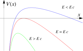
Figure 1: Shapes of the potential for some values of $E$ . The critical electric-field is denoted by $E_{\text{c}}$ . The blue line is the barrier with $E<E_{\text{c}}$ . The red line with $E=E_{\text{c}}$ . The green line with $E>E_{\text{c}}$ .

It is easy to see that there are two kinds of instabilities of the vacuum. The first instability is the tunneling process for the potential barrier. This is the usual case. When the electric field is supposed to be small as denoted with the blue line in Fig. 1, the potential barrier is present and the pair production is described as a tunneling process. As a result, the production rate is exponentially suppressed. The latter one occurs when the potential barrier vanishes. As the electric field becomes greater, the potential barrier decreases gradually. At last, it vanishes at a certain value of the electric field $E=E_{\text{c}}$ as depicted in Fig. 1. Then no tunneling occurs and the production rate is not exponentially suppressed any more. The pair production is catastrophic and the vacuum becomes totally unstable. We refer to this electric field $E_{\text{c}}$ as the critical electric-field.

If this potential analysis is true, the critical value of the external electric-field is supposed to be in QED. However, it might sound curious because such a critical value cannot be observed from the well-known results of the pair-production rate computed in QED. It is instructive to remember the formulas calculated by Schwinger [1] and Affleck-Alvarez-Manton (AAM) [2], which are given by, respectively,

$$\text{Schwinger}:~{}~{}~{} \Gamma\sim\exp\left(-\frac{\pi m^{2}}{eE}\right)\qquad\qquad~{}\text{for weak coupling and weak field}\,,$$

$$\text{AAM}:~{}~{}~{} \Gamma\sim\exp\left(-\frac{\pi m^{2}}{eE}+\frac{e^{2}}{4}\right)\qquad\text{for arbitrary coupling and weak field}\,.$$

In the Schwinger case there is no critical field trivially. In the AAM case, the exponential suppression vanishes when the electric field reaches $eE=(4\pi/e^{2})m^{2}$ . But the fine-structure constant $\alpha_{\rm s}=e^{2}/4\pi$ is around 1/137 in QED and the critical value does not satisfy the weak-field condition $eE\ll m^{2}$ . Hence the existence of the critical value is not verified.

From the above observations, the weak-field condition seems to be an obstacle to find out the critical field and hence it may be figured out if the production rate can be computed without this condition. Also, there exists the critical value of electric fields in string theory [4, 5] and this property may be regarded as a stringy nature. Hence the UV completion of the theory may be related to the critical behavior.

The AdS/CFT correspondence [6, 7, 8] provides a nice laboratory to test this argument. The holographic computation is done at strong coupling and there is no constraint for the values of external fields. This point is a great advantage in comparison to the field-theoretical computation.

Thus it is of great interesting to consider the Schwinger effect in a holographic setup and a series of studies in this direction was initiated by [9, 10]. An intriguing support for the existence of the critical electric-field has recently been presented by Semenoff and Zarembo in a holographic computation [10]. The system is the $\mathcal{N}=4$ super Yang-Mills (SYM) theory and the $U(1)$ system is realized through the Higgs mechanism. The production rate of the fundamental particles (called the W-boson supermultiplet or simply “quarks”) with mass $m$ , at large $N$ and large ’t Hooft coupling $\lambda=Ng_{\text{YM}}^{2}$ , has been computed as

$$\Gamma\sim\exp\left[-\frac{\sqrt{\lambda}}{2}\left(\sqrt{\frac{E_{\text{c}}}{E}}-\sqrt{\frac{E}{E_{\text{c}}}}\,\right)^{2}\right]\,,\qquad E_{\text{c}}=\frac{2\pi m^{2}}{\sqrt{\lambda}}\,.$$ (1.2)

The critical field $E_{\text{c}}$ can really be seen here and it also agrees with the DBI result. A generalization to the case with magnetic fields has also been done [11, 12].

On the other hand, a simple argument for the potential does not work in the above case, as noted in [10]. The critical field can be estimated by using the Coulomb potential computed with the AdS/CFT prescription [13, 14],

$$E_{\text{c}}\sim 0.70\,\frac{2\pi m^{2}}{\sqrt{\lambda}}\,.$$

This simple argument exhibits almost 30$\%$ deviation from both the string world-sheet result and the DBI result.

In this paper we revisit this deviation and reconsider the critical field from the viewpoint of the potential analysis. We examine a static potential by evaluating the classical action of a string solution attaching on a probe D3-brane sitting at an intermediate position. Then the resulting critical-field completely agrees with the DBI result. We also discuss the finite-temperature case by following [11] and show that the temperature-dependent critical-field also agrees with the DBI result.

Note that our approach has an advantage in comparison to evaluating the expectation value of circular Wilson loop. For completing the analysis in [10], the existence of a negative eigenvalue has to be shown by evaluating one-loop determinants of fluctuations around the string world-sheet solution corresponding to the circular Wilson loop [15, 16]. However, it has not been done yet because of subtleties associated with the regularization method (For attempts in this direction, see [17, 18, 19]). Our approach has no connection with the difficulty and thus our result gives a strong support for the scenario proposed in [10] from another perspective.

The organization of this paper is as follows. In section 2 a potential analysis is done at zero temperature. The Coulomb-potential part is represented by a hypergeometric function. The total potential takes a bit complicated form but the critical value of the electric field can be evaluated numerically. The result completely agrees with the one obtained from the DBI action that describes the probe D3-brane. In section 3 the finite-temperature case is investigated with the planar AdS black hole background. The temperature-dependent critical-field is examined numerically again. This result also agrees with the one obtained from the DBI action. Section 4 is devoted to conclusion and discussion.

2 Potential analysis at zero temperature

2.1 Setup

Let us introduce the setup that is necessary for our argument below. First of all, the metric of AdS${}_{5}\times$S⁵ in the Poincaré coordinates is given by

$${\rm d}s^{2}=\frac{r^{2}}{L^{2}}\,\eta_{\mu\nu}\,{\rm d}x^{\mu}{\rm d}x^{\nu}+\frac{L^{2}}{r^{2}}\,{\rm d}r^{2}+L^{2}{\rm d}\Omega_{5}^{2}\,,$$ (2.1)

where $L$ is the AdS radius and ${\rm d}\Omega_{5}^{2}$ describes S⁵ . The fundamental relation of AdS/CFT is $L^{2}/\alpha^{\prime}=\sqrt{\lambda}$ , where $\alpha^{\prime}$ is the square of string scale $\ell_{\rm s}$ like $\alpha^{\prime}\equiv\ell_{\rm s}^{2}$ . The coordinates $x^{\mu}~{}(\mu=0,\ldots,3)$ describe a four-dimensional slice for each of the values of $r$ . The metric $\eta_{\mu\nu}$ is given by

$$\eta_{\mu\nu}=\left\{\begin{array}[]{ll}{\rm{diag}}(-1,1,1,1)&\qquad\mbox{(in~{}Lorentzian)}\\ {\rm{diag}}(1,1,1,1)&\qquad\mbox{(in~{}Euclidean)}\end{array}\right.\,.$$

Depending on the purpose, the signature of $\eta_{\mu\nu}$ is taken. The critical electric-field is argued with the DBI action in the Lorentzian signature, while the static potentials are computed in the conventional way with the Euclidean signature.

Remember that a quark-antiquark potential is computed from the expectation value of a rectangular Wilson loop, where the loop is regarded as a trajectory of test particles with infinitely heavy mass. In the context of AdS/CFT, the expectation value at strong coupling can be computed with the area of a string world-sheet attaching to the Wilson loop [13, 14]. There are various ways to associate the test particles with the field-theory ingredients, depending the setup under consideration. Here the test particles are associated with the fundamental matter fields introduced by the Higgs mechanism in the $\mathcal{N}=4$ SYM via the gauge-symmetry breaking from $SU(N+1)$ to $SU(N)\times U(1)$ .

In the usual studies, the test particles are assumed to be infinitely heavy. However, this assumption is not appropriate for considering the Schwinger effect in a holographic way because the pair creation is severely suppressed due to the divergent mass. Therefore the setup should be modified so that the production rate makes sense. A resolution has been proposed by Semenoff and Zarembo [10]. It is to put a probe D3-brane at an intermediate position $r=r_{0}$ rather than close to the boundary. Then the mass $m$ becomes finite and depends on $r_{0}$ like

$$m=T_{\rm F}\,r_{0}\,,$$

where $T_{\rm F}=1/2\pi\alpha^{\prime}$ is the fundamental string tension.

Our purpose here is to compute the Coulomb potential from the area of the rectangular Wilson loop on the probe D3-brane. This computation can be done in a holographic way by evaluating the classical action of a string attaching on the probe D3-brane as depicted in Fig. 2. This is a simple analog of the analysis on the circular Wilson-loop in [10].

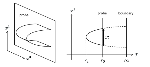
Figure 2: The setup to compute the Coulomb potential.

2.2 Potential analysis

The next step is to examine the classical solution of string world-sheet. We will work on the Euclidean signature here. Then the Nambu-Goto (NG) string action is given by

$$S = T_{\rm F}\int\!\!{\rm d}\tau\!\!\int\!\!{\rm d}\sigma\,\mathcal{L}$$ (2.2)

$$= T_{\rm F}\int\!\!{\rm d}\tau\!\!\int\!\!{\rm d}\sigma\,\sqrt{\det G_{ab}}\,,\qquad G_{ab}\equiv\frac{\partial x^{\mu}}{\partial\sigma^{a}}\frac{\partial x^{\nu}}{\partial\sigma^{b}}\,g_{\mu\nu}\,.$$

Here $G_{ab}~{}(a,b=0,1)$ is the induced metric and the world-sheet coordinates are $\sigma^{a}=(\tau,\sigma)$ . For our purpose, it is convenient to take the static gauge,

$$x^{0}=\tau\,,\qquad x^{1}=\sigma\,.$$ (2.3)

For the classical solution, suppose that the radial direction depends only on $\sigma$ ,

$$r=r(\sigma)\,,$$ (2.4)

and that the string solution is sitting at a point on S⁵ . The second condition means that a parameter $\theta^{I}$ in a Wilson loop in $\mathcal{N}=4$ SYM is a constant $\theta_{0}^{I}$ .

Under this ansatz, $\mathcal{L}$ is expressed as

$${\cal L}=\sqrt{\left(\frac{{\rm d}r}{{\rm d}\sigma}\right)^{2}+\frac{r^{4}}{L^{4}}}$$ (2.5)

and does not depend on $\sigma$ explicitly. Hence the following quantity

$$\frac{\partial{\cal L}}{\partial(\partial_{\sigma}r)}\,\partial_{\sigma}r-{\cal L}$$ (2.6)

is conserved and the relation

$$-\frac{r^{4}/L^{4}}{\displaystyle\sqrt{\left(\frac{{\rm d}r}{{\rm d}\sigma}\right)^{2}+\frac{r^{4}}{L^{4}}}}=\text{const.}$$ (2.7)

is satisfied. By imposing the boundary condition at $\sigma=0$ ,

$$\frac{{\rm d}r}{{\rm d}\sigma}=0\,,\qquad r=r_{\rm c}~{}~{}~{}~{}(r_{\rm c}<r_{0})\,,$$ (2.8)

a differential equation is derived,

$$\frac{{\rm d}r}{{\rm d}\sigma}=\frac{r^{2}}{L^{2}}\sqrt{\frac{r^{4}}{r_{\rm c}^{4}}-1}\,.$$ (2.9)

By introducing a new coordinate $y=r/r_{\rm c}$ and integrating (2.9) , the separation length $x$ of test particles on the probe brane is represented by

$$x =\frac{2L^{2}}{r_{\rm c}}\int_{1}^{r_{0}/r_{\rm c}}\frac{{\rm d}y}{y^{2}\sqrt{y^{4}-1}}$$

$$=\frac{2L^{2}}{r_{0}}\left[\frac{\sqrt{\pi}\,\Gamma(3/4)}{a\,\Gamma(1/4)}-\frac{a^{2}}{3}\,{}_{2}F_{1}\left(\frac{1}{2},\frac{3}{4},\frac{7}{4},a^{4}\right)\right]\,.$$ (2.10)

Here a dimensionless parameter $a$ is defined as

$$a\equiv\frac{r_{\rm c}}{r_{0}}\,.$$

This parameter measures the position of the tip of the classical solution with respect to the location of the probe D3-brane.

By following the setup in Fig. 2, the sum of the Coulomb potential (CP) and static energy (SE) can be estimated in a modified form like

$$V_{\rm CP+SE} =2T_{\rm F}\int^{x/2}_{0}\!\!{\rm d}r\,\mathcal{L}=2T_{\rm F}\,r_{\rm c}\int_{1}^{r_{0}/r_{\rm c}}\!{\rm d}y\,\frac{y^{2}}{\sqrt{y^{4}-1}}$$

$$=2T_{\rm F}\,r_{0}\,\left[-\frac{a\,\sqrt{\pi}\,\Gamma(3/4)}{\Gamma(1/4)}+{}_{2}F_{1}\left(-\frac{1}{4},\frac{1}{2},\frac{3}{4},a^{4}\right)\right]\,.$$ (2.11)

The Coulomb-potential part is plotted in Fig. 3.

Let us see the behavior of the potential (2.11) in the $a\to 0$ limit, which is realized by putting the probe D3-brane off to the boundary (i.e., $r_{0}\to\infty$ with $r_{\text{c}}$ fixed). With the help of the relation,

$$\lim_{a\to 0}{}_{2}F_{1}\left(-\frac{1}{4},\frac{1}{2},\frac{3}{4},a^{4}\right)=1\,,$$ (2.12)

the second term in (2.11) is reduced to the static energy of the test particles with infinitely heavy mass. Then $x$ is proportional to $1/a$ and thus the first term in (2.11) gives rise to the well-known Coulomb potential.

When $a=1$ , by using Gauss’s Hypergeometric Theorem, the second term in (2.11) can be rewritten as

$${}_{2}F_{1}\left(-\frac{1}{4},\frac{1}{2},\frac{3}{4},1\right)=\frac{\Gamma(3/4)\,\Gamma(1/2)}{\Gamma(1)\,\Gamma(1/4)}=\frac{\sqrt{\pi}\,\Gamma(3/4)}{\Gamma(1/4)}\,.$$ (2.13)

Therefore the potential (2.11) vanishes at $a=1$ . This is also obvious from the integral expression in (2.11).

What is the physical meaning of the second term in (2.11)? The potential (2.11) is finite at $x=0$ while the usual Coulomb potential diverges there (See Fig. 3). The finiteness at $x=0$ reminds us the Coulomb potential in non-linear electrodynamics. Indeed, the potential (2.11) is interpreted as the potential (+ static energy) in the DBI theory on the probe D3-brane. The short-range behavior is described by a linear potential

$$V_{\rm CP+SE}\simeq T_{\rm F}\left(\frac{r_{0}}{L}\right)^{2}x\,.$$ (2.14)

It is rather obvious that the short-distance behavior of the potential has been modified because we have cut out the UV part of the classical solution (near the boundary).

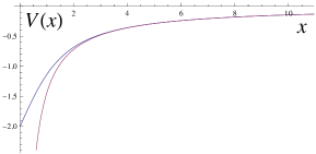
Figure 3: The modified Coulomb potential versus the usual one. The modified potential is finite even at $x=0$ , while at long distances these exhibit the same behavior. Note that the static energy is subtracted.

Let us next consider the total static-potential by turning on an electric field $E$ along the $x^{1}$-direction. It is convenient to introduce a dimensionless electric-field $\alpha$ ,

$$\alpha\equiv\frac{E}{E_{\rm c}}\,,\qquad E_{\rm c}=T_{\rm F}\,\frac{r_{0}^{2}}{L^{2}}$$ (2.15)

by measuring $E$ in a unit of the critical field $E_{\rm c}$ obtained from the DBI argument. Together with the electrostatic potential associated with $E$ , the total potential $V_{\rm tot}$ is given by

$$V_{\rm tot} =V_{\rm CP+SE}-Ex$$

$$\begin{split}&=2T_{\rm F}\,r_{0}\left\{-\frac{a\sqrt{\pi}\,\Gamma(3/4)}{\Gamma(1/4)}+{}_{2}F_{1}\left(-\frac{1}{4},\frac{1}{2},\frac{3}{4},a^{4}\right)\right.\\ &\qquad\qquad\quad\left.-\frac{\alpha}{a}\left[\frac{\sqrt{\pi}\,\Gamma(3/4)}{\Gamma(1/4)}-\frac{a^{3}}{3}\,{}_{2}F_{1}\left(\frac{1}{2},\frac{3}{4},\frac{7}{4},a^{4}\right)\right]\right\}\,.\end{split}$$ (2.16)

It seems difficult to figure out the critical value of the electric field analytically from the expression (2.16). But it is an easy task to estimate its shape numerically as a function of $x$ . The shapes for $\alpha=0.8,\,0.9,\,1.0$ and $1.1$ are plotted in Fig. 4. The potential barrier vanishes for $\alpha\geq 1.0$ and the critical field is $\alpha=1.0$ . Thus the potential (2.16) leads to the critical field that is identical with the DBI result.

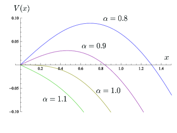
Figure 4: The shapes of the potential at zero temperature for $\alpha=0.8,\,0.9,\,1.0$ and $1.1$ are plotted from top to bottom, where $T_{\rm F}r_{0}=L^{2}/r_{0}=1$ . The potential barrier vanishes for $\alpha\geq 1.0$ and the critical field is given by $\alpha=1.0$ . Note that the behavior around $x=0$ is different from the one depicted in Fig. 1.

3 Potential analysis at finite temperature

3.1 Setup

The next subject is to consider a generalization to the finite-temperature case by following [11]. We work on the Lorentzian signature here. The metric of an AdS planar black hole is given by [24]

$${\rm d}s^{2}=-\frac{r^{2}}{L^{2}}\left(1-\frac{r_{\rm h}^{4}}{r^{4}}\right){\rm d}t^{2}+\frac{L^{2}}{r^{2}}\left(1-\frac{r_{\rm h}^{4}}{r^{4}}\right)^{-1}{\rm d}r^{2}+\frac{r^{2}}{L^{2}}\,\sum_{i=1}^{3}({\rm d}x^{i})^{2}+L^{2}{\rm d}\Omega_{5}^{2}\,.$$ (3.1)

The coordinates $x^{i}~{}(i=1,2,3)$ denote the spatial directions on a four-dimensional slice described with a fixed value of the radial coordinate $r$ . The horizon is located at $r=r_{\rm h}$ and the temperature of the black hole

$$T=\frac{r_{\rm h}}{\pi L^{2}}$$ (3.2)

is identified with that of the gauge-theory dual.

Let us consider the DBI action of a probe D3-brane on the black-hole background (3.1), including a constant, world-volume electric-field $E$ . The probe D3-brane is located at $r=r_{0}$ and the following relation is assumed below:

$$r_{\rm h}<r_{\rm c}<r_{0}\,.$$

The classical action is written into the form,

$$S =-T_{\text{D3}}\int\!\!{\rm d}^{4}x\,\sqrt{-\det(g_{\mu\nu}+{\cal F}_{\mu\nu})}$$

$$=-T_{\text{D3}}\frac{r_{0}^{4}}{L^{4}}\sqrt{1-\frac{r_{\rm h}^{4}}{r_{0}^{4}}}\int\!\!{\rm d}^{4}x\,\sqrt{1-\frac{(2\pi\alpha^{\prime})^{2}L^{4}}{r_{0}^{4}(1-r_{\rm h}^{4}/r_{0}^{4})}E^{2}}\,,$$ (3.3)

where $T_{\text{D3}}$ is the D3-brane tension given by

$$T_{\text{D3}}=\frac{1}{g_{\text{s}}(2\pi)^{3}\alpha^{\prime 2}}\,.$$

The DBI action becomes ill-defined for $E>E_{\text{c}}$ , where $E_{\text{c}}$ is the critical value given by

$$E_{\text{c}}=T_{\rm F}\frac{r_{0}^{2}}{L^{2}}\,\sqrt{1-\frac{r_{\rm h}^{4}}{r_{0}^{4}}}\,.$$ (3.4)

One can see that $E_{\text{c}}$ implicitly depends on the temperature.

It is instructive to rewrite the mass of the fundamental matter in terms of the gauge-theory parameters and see the temperature dependence of $E_{\text{c}}$ . The induced metric on the string world-sheet is

$$g_{ab}={\rm{diag}}\left(-\frac{r^{2}}{L^{2}}\left(1-r_{\rm h}^{4}/r^{4}\right),\frac{L^{2}}{r^{2}}(1-r_{\rm h}^{4}/r^{4})^{-1}\right)$$ (3.5)

and then the mass is represented by

$$m=T_{\rm F}\int_{r_{\rm h}}^{r_{0}}\!{\rm d}r\,\sqrt{-\det g_{ab}}\,=T_{\rm F}\left(r_{0}-r_{\rm h}\right)\,.$$ (3.6)

Thus the mass also depends on the temperature. It is notable that the temperature dependence comes from the integration range rather than the induced metric (3.5).

The temperature-dependent mass $m(T)$ is written into the well-known form,

$$m(T)=m(T=0)+\Delta m(T)\equiv m(T=0)-\frac{\sqrt{\lambda}}{2}T\,.$$ (3.7)

Then $E_{\text{c}}$ is also expressed in terms of the gauge-theory parameters as

$$E_{\text{c}}(T) = \frac{2\pi m^{2}}{\sqrt{\lambda}}\sqrt{\left(1-\frac{\Delta m(T)}{m}\right)^{4}-\left(\frac{\Delta m(T)}{m}\right)^{4}}$$ (3.8)

$$\simeq \frac{2\pi m^{2}}{\sqrt{\lambda}}\left(1-2\frac{\Delta m(T)}{m}\right)+\mathcal{O}\left(\frac{\Delta m(T)}{m}\right)\qquad(m\gg\sqrt{\lambda}\,T)\,.$$

It is worth noting that $E_{\text{c}}$ is well defined for arbitrary values of $T$ .

3.2 Potential analysis

The analysis on the classical solution is similar to the zero-temperature case. We work on the Euclidean signature here. The ansatz for the solution is also not changed. The induced metric $G_{ab}$ is slightly modified and the NG action is rewritten as

$$S=T_{\rm F}\int\!\!{\rm d}\tau\!\int\!\!{\rm d}\sigma\,{\cal L}\,,\qquad{\cal L}=\sqrt{\left(\frac{{\rm d}r}{{\rm d}\sigma}\right)^{2}+\frac{r^{4}}{L^{4}}\left(1-\frac{r_{\rm h}^{4}}{r^{4}}\right)}\,.$$ (3.9)

The quantity in (2.6) is conserved again and the relation

$$-\frac{r^{4}/L^{4}}{\displaystyle\sqrt{\left(\frac{{\rm d}r}{{\rm d}\sigma}\right)^{2}+\frac{r^{4}}{L^{4}}\left(1-\frac{r_{\rm h}^{4}}{r^{4}}\right)}}\left(1-\frac{r_{\rm h}^{4}}{r^{4}}\right)=\text{const.}$$ (3.10)

is satisfied. By imposing the boundary condition (2.8) at $\sigma=0$ again, we obtain the following differential equation,

$$\frac{{\rm d}r}{{\rm d}\sigma}=\frac{r^{2}}{L^{2}}\sqrt{\left(1-\frac{r_{\rm h}^{4}}{r^{4}}\right)\frac{r^{4}-r_{\rm c}^{4}}{r_{\rm c}^{4}-r_{\rm h}^{4}}}\,.$$ (3.11)

Integrating (3.11), the distance $x$ between the test particles is represented by the following integral,

$$x=\frac{2L^{2}}{r_{0}}\frac{1}{a}\sqrt{1-\frac{b^{4}}{a^{4}}}\int_{1}^{1/a}\!\frac{{\rm d}y}{\sqrt{(y^{4}-1)(y^{4}-b^{4}/a^{4})}}\,.$$ (3.12)

Here we have introduced the following dimensionless quantities:

$$y=\frac{r}{r_{\rm c}}\,,\qquad a=\frac{r_{\rm c}}{r_{0}}\,,\qquad b=\frac{r_{\rm h}}{r_{0}}\,.$$

The sum of the Coulomb potential between the fundamental fields and the static energy is given by

$$V_{\rm CP+SE}=2T_{\rm F}\int_{0}^{x/2}\!{\rm d}\sigma\,{\cal L}=2T_{\rm F}\,r_{0}\,a\int_{1}^{1/a}\!{\rm d}y\,\sqrt{\frac{y^{4}-b^{4}/a^{4}}{y^{4}-1}}\,.$$ (3.13)

Let us next turn on an electric field $E$ along the $x^{1}$-direction. It can be measured with respect to the critical value (3.4) by using a dimensionless parameter $\alpha$ like

$$\alpha=\frac{E}{E_{\rm c}(T)}\,,$$

where $E_{\rm c}(T)$ is the critical field determined by the DBI argument and is given in (3.4). Then the total potential $V_{\rm tot}$ is given by

$$V_{\rm tot} =V_{\rm CP+SE}-Ex$$

$$\begin{split}&=2T_{\rm F}\,r_{0}\left[~{}a\int_{1}^{1/a}\!{\rm d}y\,\sqrt{\frac{y^{4}-b^{4}/a^{4}}{y^{4}-1}}\right.\\ &\qquad\qquad\left.-\frac{1}{a}\sqrt{(1-b^{4})\left(1-\frac{b^{4}}{a^{4}}\right)}\int_{1}^{1/a}\!\frac{{\rm d}y}{\sqrt{(y^{4}-1)(y^{4}-b^{4}/a^{4})}}\right]\,.\end{split}$$ (3.14)

What we can do at most is to evaluate the potential shape (3.14) numerically again. The shapes of the potential (3.14) with a fixed temperature $b=0.5$ are plotted for the values $\alpha=0.8,\,0.9,\,1.0$ and $1.1$ in Fig. 5. The potential barrier vanishes for $\alpha\geq 1.0$ and the critical field is $\alpha=1.0$ again. Thus the critical field agrees with the DBI result.

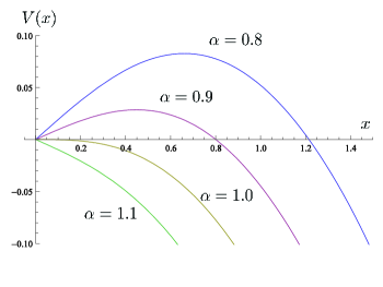
Figure 5: The shapes of the potential with a fixed temperature ($b=0.5$) are plotted for $\alpha=0.8,\,0.9,\,1.0$ and $1.1$ from top to bottom, where $T_{\rm F}r_{0}=L^{2}/r_{0}=1$. The potential barrier vanishes for $\alpha\geq 1.0$ and the critical field is $\alpha=1.0$ .

It should be remarked here that there is a degeneracy between the distance $x$ and the auxiliary parameter $a$ at finite temperature (while no degeneracy at zero temperature). The distance $x$ is plotted against $a$ for $b=0$ and $0.5$ in Fig. 6. The value of $x$ is uniquely determined for a given value of $a$ at zero temperature ($b=0$), while a single value of $x$ corresponds to two values of $a$ at finite temperature. Therefore the region of $a$ has to be restricted for numerical computations. In fact, the branch with smaller values of $a$ means the region close to the horizon and describes another configuration of string world-sheet, a pair of straight Wilson lines, as discussed in [25]. Thus the branch with larger values of $a$ has been taken for the present analysis. For Fig. 5 , the range between 0.6 and 1.0 is utilized.

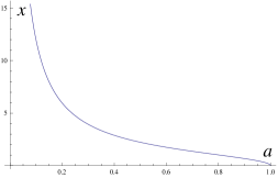
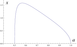
$b=0$	$b=0.5$

Figure 6: The distance $x$ is plotted against $a$ for $b=0$ and $b=0.5$ .

4 Conclusion and discussion

We have analyzed electrostatic potentials in the holographic Schwinger effect by evaluating the classical action of a string solution attaching on a probe D3-brane sitting at an intermediate position in the bulk AdS. It has been shown numerically that the resulting critical-field agrees with the DBI result and the 30$\%$ deviation denoted in Introduction has been resolved. This agreement gives a strong support for the scenario proposed in [10]. The finite-temperature case has also been considered with the planar AdS black hole. We have shown numerically that the temperature-dependent critical-field also agrees with the DBI result.

It is also nice to consider the holographic Schwinger effect in the D3/D7-branes system. The pair creation of quark and antiquark and its time evolution are discussed in [26, 27] (For a review on quark dynamics in the holographic approach, for example, see [28]). It would not be difficult to follow our approach in the D3/D7-branes system and it is interesting to consider the relation between the critical field and the time evolution of quark-antiquark pairs. We hope that we could report on this issue in the near future.

References

- [1] J. S. Schwinger, “On gauge invariance and vacuum polarization,” Phys. Rev. 82 (1951) 664.
- [2] I. K. Affleck, O. Alvarez and N. S. Manton, “Pair Production At Strong Coupling In Weak External Fields,” Nucl. Phys. B 197 (1982) 509.
- [3] I. K. Affleck and N. S. Manton, “Monopole Pair Production In A Magnetic Field,” Nucl. Phys. B 194 (1982) 38.
- [4] E. S. Fradkin and A. A. Tseytlin, “Quantum String Theory Effective Action,” Nucl. Phys. B 261 (1985) 1.
- [5] C. Bachas and M. Porrati, “Pair creation of open strings in an electric field,” Phys. Lett. B 296 (1992) 77 [hep-th/9209032].
- [6] J. M. Maldacena, “The large N limit of superconformal field theories and supergravity,” Adv. Theor. Math. Phys. 2 (1998) 231 [Int. J. Theor. Phys. 38 (1999) 1113]. [arXiv:hep-th/9711200].
- [7] S. S. Gubser, I. R. Klebanov and A. M. Polyakov, “Gauge theory correlators from non-critical string theory,” Phys. Lett. B 428 (1998) 105 [arXiv:hep-th/9802109].
- [8] E. Witten, “Anti-de Sitter space and holography,” Adv. Theor. Math. Phys. 2 (1998) 253 [arXiv:hep-th/9802150].
- [9] A. S. Gorsky, K. A. Saraikin and K. G. Selivanov, “Schwinger type processes via branes and their gravity duals,” Nucl. Phys. B 628 (2002) 270 [hep-th/0110178].
- [10] G. W. Semenoff and K. Zarembo, “Holographic Schwinger Effect,” Phys. Rev. Lett. 107 (2011) 171601 [arXiv:1109.2920 [hep-th]].
- [11] S. Bolognesi, F. Kiefer and E. Rabinovici, “Comments on Critical Electric and Magnetic Fields from Holography,” JHEP 1301 (2013) 174 [arXiv:1210.4170 [hep-th]].
- [12] Y. Sato and K. Yoshida, “Holographic description of the Schwinger effect in electric and magnetic fields,” JHEP 1304 (2013) 111 [arXiv:1303.0112 [hep-th]].
- [13] S. -J. Rey and J. -T. Yee, “Macroscopic strings as heavy quarks in large N gauge theory and anti-de Sitter supergravity,” Eur. Phys. J. C 22 (2001) 379 [hep-th/9803001].
- [14] J. M. Maldacena, “Wilson loops in large N field theories,” Phys. Rev. Lett. 80 (1998) 4859 [hep-th/9803002].
- [15] D. E. Berenstein, R. Corrado, W. Fischler and J. M. Maldacena, “The Operator product expansion for Wilson loops and surfaces in the large N limit,” Phys. Rev. D 59 (1999) 105023 [hep-th/9809188].
- [16] N. Drukker, D. J. Gross and H. Ooguri, “Wilson loops and minimal surfaces,” Phys. Rev. D 60 (1999) 125006 [hep-th/9904191].
- [17] N. Drukker, D. J. Gross and A. A. Tseytlin, “Green-Schwarz string in AdSS5: Semiclassical partition function,” JHEP 0004 (2000) 021 [hep-th/0001204].
- [18] J. Ambjorn and Y. Makeenko, “Remarks on Holographic Wilson Loops and the Schwinger Effect,” Phys. Rev. D 85 (2012) 061901 [arXiv:1112.5606 [hep-th]].
- [19] C. Kristjansen and Y. Makeenko, “More about One-Loop Effective Action of Open Superstring in AdSS5,” JHEP 1209 (2012) 053 [arXiv:1206.5660 [hep-th]].
- [20] D. N. Kabat and G. Lifschytz, “A Note on the Coulomb branch of SUSY Yang-Mills,” Phys. Lett. B 633 (2006) 641 [hep-th/0511226].
- [21] D. H. Delphenich, “Nonlinear electrodynamics and QED,” hep-th/0309108.
- [22] M. Kruczenski, D. Mateos, R. C. Myers and D. J. Winters, “Meson spectroscopy in AdS / CFT with flavor,” JHEP 0307 (2003) 049 [hep-th/0304032].
- [23] Y. Sato and K. Yoshida, “Holographic Schwinger effect in confining phase,” arXiv:1306.5512 [hep-th].
- [24] G. T. Horowitz and A. Strominger, “Black strings and P-branes,” Nucl. Phys. B 360 (1991) 197.
- [25] S. -J. Rey, S. Theisen and J. -T. Yee, “Wilson-Polyakov loop at finite temperature in large N gauge theory and anti-de Sitter supergravity,” Nucl. Phys. B 527 (1998) 171 [hep-th/9803135].
- [26] C. P. Herzog, A. Karch, P. Kovtun, C. Kozcaz and L. G. Yaffe, “Energy loss of a heavy quark moving through N=4 supersymmetric Yang-Mills plasma,” JHEP 0607 (2006) 013 [hep-th/0605158].
- [27] M. Chernicoff and A. Guijosa, “Acceleration, Energy Loss and Screening in Strongly-Coupled Gauge Theories,” JHEP 0806 (2008) 005 [arXiv:0803.3070 [hep-th]].
- [28] M. Chernicoff, J. A. Garcia, A. Guijosa and J. F. Pedraza, “Holographic Lessons for Quark Dynamics,” J. Phys. G 39 (2012) 054002 [arXiv:1111.0872 [hep-th]].