Introduction

Black hole physics is an extremely active research field in String Theory. Some impressive results have been obtained towards a complete match of the microscopic and the macroscopic entropies of extremal black holes [1] beyond leading order, see [2, 3] and references therein. So far, most of the literature has been focused on the so called higher-order (curvature) corrections [4, 5, 6, 7, 8]. These modify the usual Bekenstein-Hawking area law

$$S=\frac{A}{4}\,,$$

and are prescribed by String Theory to appear in the effective classical Supergravity description. In the context of Type-IIA, the effective theory is described by a two-derivative Supergravity at tree level in $g_{s}$, with the higher-order corrections ocurring already at the 1-loop level.

There exist, however, a different type of stringy corrections (which correct the point particle behaviour), some of which do not modify the effective Lagrangian of Type-IIA String Theory with higher order terms, but modify the couplings and the scalar manifold geometry of the classical Supergravity action. These are the $\alpha^{\prime}$-corrections, often referred to as quantum corrections, at least in the context of Type-IIA Calabi-Yau (C.Y.) compactifications [9, 10, 11, 12]. In contradistinction to the curvature ones, these do not modify the Bekenstein-Hawking area law.

It turns out that not so much attention has been paid to the effects of these quantum corrections to black hole solutions of the classical Supergravity action. Some exceptions, in which this kind of solutions (or their corresponding critical points) in the presence of these have been considered, are [13, 14, 15, 16, 17, 18, 19].

In [20], using the H-FGK formalism [23, 24, 25, 26], a new class of black holes for Type-IIA C.Y. compactifications was defined: they exist only when the perturbative corrections to the prepotential are included and no classical limit can be assigned to them. They were called, in consequence, quantum black holes. Therefore, for self-mirror C.Y. manifolds such black holes do not exist, since in such case the perturbative corrections exactly vanish. However, the situation can be changed if we add non-perturbative corrections to the prepotential. That is the case we are going to consider in this letter. We will obtain the first explicit black hole solution of Type-IIA String Theory compactified on a self-mirror Calabi-Yau threefold in the presence of non-perturbative corrections, proving at the same time that these non-perturbative corrections lift the singular behaviour of the quantum black holes to a regular one.

The solution (general class of solutions, in fact) may allow also for an explicit check of the match between the microscopic String Theory entropy and the macroscopic entropy of a supersymmetric black hole solution in the presence of these non-perturbative corrections. To that respect, some partial results can be found in [13]. In any case, computing the macroscopic solution is undoubtedly the first step towards the resolution of this puzzle.

Somewhat surprisingly, we obtain a class of solutions which involves Lambert’s W function [27], which is multi-valued in a certain real domain. We will explain how this fact seems to provide an appropriate scenario for a potential violation of the (corresponding uniqueness conjecture, and as a consequence of the) No-Hair conjecture in four dimensions. It turns out that, in our set-up, String Theory forbids the use of the Lambert function to that end. However, the possibility remains open in an exclusive Supergravity set-up (not necessarily embedded in String Theory) [28], and there does not seem to be a reason to discard it right away. Black holes in ungauged four-dimensional Supergravity still hold some surprises [29, 30], which indicate that we may not completely understand them even in the extremal case.

Finally, it would also be of major interest to extend the construction of quantum black holes to the case of multicentered configurations [31, 32, 33, 34, 35, 36, 37, 38, 39, 40, 41, 42, 43, 44].

1 Type-IIA String Theory on a Calabi–Yau manifold

Type-IIA String Theory compactified to $4$D on a C.Y. three-fold, with Hodge numbers $(h^{1,1},h^{2,1})$, is described, up to two derivatives, by a $\mathcal{N}=2,d=4$ Supergravity whose prepotential is given in terms of an infinite series around $\Im{\rm m}z^{i}\rightarrow\infty$[45, 10, 9]

$$\mathcal{F}=-\frac{1}{3!}\kappa^{0}_{ijk}z^{i}z^{j}z^{k}+\frac{ic}{2}+\frac{i}{(2\pi)^{3}}\sum_{\{d_{i}\}}n_{\{d_{i}\}}Li_{3}\left(e^{2\pi id_{i}z^{i}}\right)\ \,,$$ (1.1)

where $z^{i},~{}~{}i=1,...,n_{v}+1=h^{1,1}$, are the scalars in the vector multiplets. There are also $h^{2,1}+1$ hypermultiplets in the theory. However, they can be consistently set to a constant value (See [46], section 3.2). $c=\frac{\chi\zeta(3)}{(2\pi)^{3}}$ is a model-dependent number, being $\chi$ the Euler characteristic, which for C.Y. three-folds is given by $\chi=2(h^{1,1}-h^{2,1})$. $\kappa^{0}_{ijk}$ are the classical intersection numbers, $d_{i}\in\mathbb{Z}^{+}$ is a $h^{1,1}$-dimensional summation index and $Li_{3}(x)$ is the third polylogarithmic function, defined in appendix A. The first two terms in the prepotential correspond to tree level and loop perturbative contributions in the $\alpha^{\prime}$-expansion, respectively

$$\mathcal{F}_{\text{P}}=-\frac{1}{3!}\kappa^{0}_{ijk}z^{i}z^{j}z^{k}+\frac{ic}{2}\ \,,$$ (1.2)

whereas the third term accounts for non-perturbative corrections produced by world-sheet instantons. These configurations get produced by (non-trivial) embeddings of the world-sheet into the C.Y. three-fold. The holomorphic mappings of the genus 0 string world-sheet onto the $h^{1,1}$ two-cycles of the C.Y. three-fold are classified by the nubers $d_{i}$, which count the number of wrappings of the world-sheet around the $i-$th generator of the integer homology group $H_{2}(\text{C.Y.},\mathbb{Z})$. The number of different mappings for each set of $\{d_{i}\}$ $\left(\equiv\{d_{1},...,d_{h^{1,1}}\}\right)$ or, in other words, the number of genus $0$ instantons is denoted by $n_{\{d_{i}\}}$

$$\mathcal{F}_{\text{NP}}=\frac{i}{(2\pi)^{3}}\sum_{\{d_{i}\}}n_{\{d_{i}\}}Li_{3}\left(e^{2\pi id_{i}z^{i}}\right)\ \,.$$ (1.3)

The full prepotential can be rewritten in homogeneous coordinates $\mathcal{X}^{\Lambda}$, $\Lambda=(0,i)$ as

$$F(\mathcal{X})=-\frac{1}{3!}\kappa^{0}_{ijk}\frac{\mathcal{X}^{i}\mathcal{X}^{j}\mathcal{X}^{k}}{\mathcal{X}^{0}}+\frac{ic(\mathcal{X}^{0})^{2}}{2}+\frac{i(\mathcal{X}^{0})^{2}}{(2\pi)^{3}}\sum_{\{d_{i}\}}n_{\{d_{i}\}}Li_{3}\left(e^{2\pi id_{i}\frac{\mathcal{X}^{i}}{\mathcal{X}^{0}}}\right)\ \,,$$ (1.4)

with the scalars $z^{i}$ given by

$$z^{i}=\frac{\mathcal{X}^{i}}{\mathcal{X}^{0}}\ \,.$$ (1.5)

Therefore, this coordinate system is only valid away from the locus $\mathcal{X}^{0}=0$.

We are interested in studying spherically symmetric, static, black hole solutions of the theory defined by Eq. (1.1). In order to do so we are going to use the so-called H-FGK, developed in [23, 24, 25], based on the use of a new set of variables $H^{M},~{}~{}M=(\Lambda,\Lambda)$, which transform linearly under duality and reduce to harmonic functions on the transverse space $\mathbb{R}^{3}$ in the supersymmetric case.

2 A non-perturbative class of black holes

The most general static, spherically symmetric space-time metric solution of an ungauged Supergravity is given by [47, 24]

$$\begin{array}[]{rcl}ds^{2}&=&e^{2U(\tau)}dt^{2}-e^{-2U(\tau)}\gamma_{\underline{m}\underline{n}}dx^{\underline{m}}dx^{\underline{n}}\,,\\ &&\\ \gamma_{\underline{m}\underline{n}}dx^{\underline{m}}dx^{\underline{n}}&=&{\displaystyle\frac{r_{0}^{4}}{\sinh^{4}r_{0}\tau}}d\tau^{2}+{\displaystyle\frac{r_{0}^{2}}{\sinh^{2}r_{0}\tau}}d\Omega^{2}_{(2)}\,.\\ \end{array}$$ (2.1)

Using Eq. (2.1), and assuming spherical symmetry for all the fields in the theory, the equations of motion of the bosonic sector of $\mathcal{N}=2$, $d=4$ Supergravity can be written as a set of ordinary differential equations (in the variable $\tau$) for the scalars $z^{i}(\tau)$, $i=1,...,n_{v}$ and the metric warp factor $U(\tau)$ [47]. The vector fields do not appear in these equations since they can be explicitly integrated in terms of the corresponding electric and magnetic charges.

The one dimensional effective equations of motion can be recast in a duality covariant way by performing a particular change of variables to a new set of $(2n_{v}+2)$ variables $H^{M}(\tau)$ which transform linearly under the U-duality group of the theory, and become harmonic functions in $\mathbb{R}^{3}$ in the supersymmetric case. This is the essence of the H-FGK formalism [23, 24, 25, 26], whose equations of motion read
( $\dot{}\equiv\frac{d}{d\tau}$)

$$\mathcal{E}_{P}=\tfrac{1}{2}\partial_{P}\partial_{M}\partial_{N}\log\mathsf{W}\,\left[\dot{H}^{M}\dot{H}^{N}-\tfrac{1}{2}\mathcal{Q}^{M}\mathcal{Q}^{N}\right]+\partial_{P}\partial_{M}\log\mathsf{W}\,\ddot{H}^{M}-\frac{d}{d\tau}\left(\frac{\partial\Lambda}{\partial\dot{H}^{P}}\right)+\frac{\partial\Lambda}{\partial H^{P}}=0\,,$$ (2.3)

together with the Hamiltonian constraint

$$\mathcal{H}\equiv-\tfrac{1}{2}\partial_{M}\partial_{N}\log\mathsf{W}\left(\dot{H}^{M}\dot{H}^{N}-\tfrac{1}{2}\mathcal{Q}^{M}\mathcal{Q}^{N}\right)+\left(\frac{\dot{H}^{M}H_{M}}{\mathsf{W}}\right)^{2}-\left(\frac{\mathcal{Q}^{M}H_{M}}{\mathsf{W}}\right)^{2}-r_{0}^{2}=0\,,$$ (2.4)

where

$$\Lambda\equiv\left(\frac{\dot{H}^{M}H_{M}}{\mathsf{W}}\right)^{2}+\left(\frac{\mathcal{Q}^{M}H_{M}}{\mathsf{W}}\right)^{2}\,,$$ (2.5)

and

$$\mathsf{W}(H)\equiv\tilde{H}_{M}(H)H^{M}=e^{-2U},~{}~{}~{}\tilde{H}^{M}+i\mathcal{I}^{M}=\mathcal{V}^{M}/X\,.$$ (2.6)

$\mathcal{V}^{M}$ is the covariantly holomorphic symplectic section of $\mathcal{N}=2$ Supergravity, and $X$ is a complex variable with the same Kähler weight as $\mathcal{V}^{M}$. $\tilde{H}^{M}(\mathcal{I})\equiv\tilde{H}^{M}(H)$ stands for the real part $\left(\tilde{H}^{M}\right)$ of $\mathcal{V}^{M}$ written as a function of the imaginary part $\mathcal{I}^{M}\equiv H^{M}$, something that can always be done by solving the so-called stabilization equations, which we will explicitly write down in a moment. $\mathsf{W}(H)$ is usually known in the literature as the Hesse potential.

The effective theory is now expressed in terms of $2\left(n_{v}+1\right)$ variables $H^{M}$ and depends on $2\left(n_{v}+1\right)+1$ parameters: $2\left(n_{v}+1\right)$ charges $\mathcal{Q}^{M}=\left(p^{\Lambda},\,\,q_{\Lambda}\right)^{T}$ and the non-extremality parameter $r_{0}$, from which it is possible to reconstruct the solution in terms of the original fields of the theory (that is it, the space-time metric, scalars and vector fields).

In order to tackle the construction of new black hole solutions of (1.1), we are going to consider a particular consistent truncation given by

$$H^{0}=H_{0}=H_{i}=0,~{}~{}p^{0}=q_{0}=q_{i}=0\,.$$ (2.7)

Under this assumption, the stabilization equations, which can be directly read off from (2.6) take the form

$$\left(\begin{array}[]{c}iH^{i}\\ \tilde{H}_{i}\end{array}\right)=\frac{e^{\mathcal{K}/2}}{X}\left(\begin{array}[]{c}\mathcal{X}^{i}\\ \frac{\partial F(\mathcal{X})}{\partial\mathcal{X}^{i}}\end{array}\right)\,,\left(\begin{array}[]{c}\tilde{H}^{0}\\ 0\end{array}\right)=\frac{e^{\mathcal{K}/2}}{X}\left(\begin{array}[]{c}\mathcal{X}^{0}\\ \frac{\partial F(\mathcal{X})}{\partial\mathcal{X}^{0}}\end{array}\right),$$ (2.8)

where we have used that the covariantly holomorphic symplectic section $\mathcal{V}^{M}$ can be written as follows [49]

$$\mathcal{V}^{M}=e^{\mathcal{K}/2}\left(\mathcal{X}^{\Lambda},\,\,\partial_{\Lambda}F(\mathcal{X})\right)\,.$$ (2.9)

The physical fields can be obtained from the $H^{i}$ as

$$e^{-2U}=\tilde{H}_{i}H^{i}\,,~{}~{}z^{i}=i\frac{H^{i}}{\tilde{H}^{0}}\,,$$ (2.10)

as soon as $\tilde{H}^{0}$ and $\tilde{H}^{i}$ are determined. In order to obtain $\tilde{H}^{0}$ as a function of $H^{i}$, we need to solve the highly involved equation

$$\frac{\partial{F(H)}}{\partial\tilde{H}^{0}}=0\,,$$ (2.11)

where $F(H)$ stands for the prepotential expressed in terms of the $H^{i}$

$$F(H)=\frac{i}{3!}\kappa^{0}_{ijk}\frac{H^{i}H^{j}H^{k}}{\tilde{H}^{0}}+\frac{ic(\tilde{H}^{0})^{2}}{2}+\frac{i(\tilde{H}^{0})^{2}}{(2\pi)^{3}}\sum_{\{d_{i}\}}n_{\{d_{i}\}}Li_{3}\left(e^{-2\pi d_{i}\frac{H^{i}}{\tilde{H}^{0}}}\right)\,.$$ (2.12)

Once this is done, it is not difficult to express $\tilde{H}^{i}$ in terms of $H^{i}$. Indeed, from (2.8) we simply have

$$\tilde{H}_{i}=-i\frac{\partial{F(H)}}{\partial H^{i}}\,.$$ (2.13)

If we expand (2.11), we find

$$-\frac{1}{3!}\kappa^{0}_{ijk}\frac{H^{i}H^{j}H^{k}}{({\tilde{H}^{0}})^{3}}+c+\frac{1}{4\pi^{3}}\sum_{\{d_{i}\}}n_{\{d_{i}\}}\left[Li_{3}\left(e^{-2\pi d_{i}\frac{H^{i}}{\tilde{H}^{0}}}\right)\right.\left.+Li_{2}\left(e^{-2\pi d_{i}\frac{H^{i}}{\tilde{H}^{0}}}\right)\left[\frac{\pi d_{i}H^{i}}{\tilde{H}^{0}}\right]\right]=0\,.$$ (2.14)

Solving (2.14) for $\tilde{H}^{0}$ in full generality seems to be an extremely difficult task. However, if we go to the large volume compactification limit ($\Im{\rm m}z^{i}>>1$), we can make use of the following property of the polylogarithmic functions

$$\lim_{|w|\rightarrow 0}Li_{s}(w)=w\,,\forall s\in\mathbb{N}\,,$$ (2.15)

since, in our case, $w=e^{-2\pi d_{i}\Im mz^{i}}\,,\forall\left\{d_{i}\right\}\in\left(\mathbb{Z}^{+}\right)^{h^{1,1}}$. Eq. (2.15) enables us to rewrite (2.14) as

$$-\frac{1}{3!}\kappa^{0}_{ijk}\frac{H^{i}H^{j}H^{k}}{({\tilde{H}^{0}})^{3}}+c+\frac{1}{4\pi^{3}}\sum_{\{d_{i}\}}n_{\{d_{i}\}}\left[e^{-2\pi d_{i}\frac{H^{i}}{\tilde{H}^{0}}}\right.\left.+e^{-2\pi d_{i}\frac{H^{i}}{\tilde{H}^{0}}}\left[\frac{\pi d_{i}H^{i}}{\tilde{H}^{0}}\right]\right]=0\,,~{}~{}\Im{\rm m}z^{i}>>1\,.$$ (2.16)

The dominant contribution in this regime, aside from the cubic one, is given by $c$. In [20] [17], the first non-extremal black hole solutions (with constant and non-constant scalars) of (1.1) were obtained ignoring the non-perturbative corrections. In particular, the solutions of [20] turned out to be purely quantum, in the sense that not only the classical limit $c\rightarrow 0$ was ill-defined, but also the truncated theory became inconsistent and therefore no classical limit could be assigned to such solutions. An interesting question to ask now is whether the non-perturbative contributions could actually be able to cure or at least improve this behaviour. On the other hand, it is also interesting per se to explore the existence of black hole solutions when the subleading contribution to the prepotential is not given by $c$, but has a non-perturbative origin. In order to tackle these two questions, let us restrict ourselves to C.Y. three-folds with vanishing Euler characteristic ($c=0$), the so-called self-mirror C.Y. three-folds. Under this assumption, and considering only the subleading contribution in (2.14), which is now given by the fourth term in (2.16), such equation becomes

$$-\frac{1}{3!}\kappa^{0}_{ijk}\frac{H^{i}H^{j}H^{k}}{({\tilde{H}^{0}})^{3}}+\frac{1}{4\pi^{3}}\sum_{\{d_{i}\}}n_{\{d_{i}\}}e^{-2\pi d_{i}\frac{H^{i}}{\tilde{H}^{0}}}\left[\frac{\pi d_{i}H^{i}}{\tilde{H}^{0}}\right]=0\,.$$ (2.17)

The sum over $\{d_{i}\}$ in (2.17) will be dominated in each case by a certain term corresponding to a particular vector $\left\{\hat{d}_{i}\right\}$ (and, as a consequence, to a particular $n_{\hat{d}_{i}}\equiv\hat{n}$), which, since we are assuming $\Im{\rm m}z^{i}>>1$, is the only one that we need to consider. That is, $\left\{\hat{d}_{i}\right\}$ corresponds to the set of $d_{i}$ that labels the most relevant term in the infinite sum present in (2.17). Hence, this equation becomes

$$-\frac{1}{3!}\kappa^{0}_{ijk}\frac{H^{i}H^{j}H^{k}}{({\tilde{H}^{0}})^{3}}+\frac{\hat{n}}{4\pi^{3}}e^{-2\pi\hat{d}_{i}\frac{H^{i}}{\tilde{H}^{0}}}\left[\frac{\pi\hat{d}_{i}H^{i}}{\tilde{H}^{0}}\right]=0\,,~{}~{}\Im{\rm m}z^{i}>>1\,.$$ (2.18)

This is solved by

$$\tilde{H}^{0}=\frac{\pi\hat{d}_{l}H^{l}}{W_{a}\left(s_{a}\sqrt{\frac{3\hat{n}(\hat{d}_{n}H^{n})^{3}}{2\kappa^{0}_{ijk}H^{i}H^{j}H^{k}}}\right)}\,,$$ (2.19)

where $W_{a}(x),~{}(a=0,-1)$ stands for (any of the two real branches of) the Lambert $W$ function (also known as product logarithm), and $s_{a}=\pm 1$. Using now Eqs. (2.19) and (2.13) we can obtain $\tilde{H}^{i}$. The result is

$$\tilde{H}_{i}=\frac{1}{2}\kappa^{0}_{ijk}\frac{H^{j}H^{k}}{\pi\hat{d}_{l}H^{l}}W_{a}\left(s_{a}\sqrt{\frac{3\hat{n}(\hat{d}_{m}H^{m})^{3}}{2\kappa^{0}_{pqr}H^{p}H^{q}H^{r}}}\right)\,.$$ (2.20)

The physical fields can now be written as a function of the $H^{i}$ as

$$e^{-2U}=\mathsf{W}(H)=\frac{\kappa^{0}_{ijk}H^{i}H^{j}H^{k}}{2\pi\hat{d}_{m}H^{m}}W_{a}\left(s_{a}\sqrt{\frac{3\hat{n}(\hat{d}_{l}H^{l})^{3}}{2\kappa^{0}_{pqr}H^{p}H^{q}H^{r}}}\right)\,,$$ (2.21)

$$z^{i}=i\frac{H^{i}}{\pi\hat{d}_{m}H^{m}}W_{a}\left(s_{a}\sqrt{\frac{3\hat{n}(\hat{d}_{l}H^{l})^{3}}{2\kappa^{0}_{pqr}H^{p}H^{q}H^{r}}}\right)\,.$$ (2.22)

In order to have a regular solution, we need to have a positive definite metric warp factor $e^{-2U}$. Since, as explained in Appendix B, ${\rm sign}\left[W_{a}(x)\right]={\rm sign}\left[x\right],~{}a=0,-1,~{}x\in D^{a}_{\mathbb{R}}$, we have to require that

$$s_{0}\equiv sign\left[\kappa^{0}_{ijk}\frac{H^{i}H^{j}H^{k}}{\hat{d}_{m}H^{m}}\right]\,,$$ (2.23)

$$s_{-1}\equiv-1\,.$$ (2.24)

On the other hand, since $W_{0}(x)=0$ for $x=0$ and $W_{-1}(x)$ is a real function only when $x\in\left[-\frac{1}{e},0\right)$, we have to impose that the argument $x$ of $W_{a}$ lies entirely either in $\left[-\frac{1}{e},0\right)$ or in $\left(0,\infty\right)$ for all $\tau\in\left(-\infty,0\right)$, since $e^{2U}$ cannot be zero in a regular black hole solution for any $\tau\in\left(-\infty,0\right)$. This condition must be imposed in a case by case basis, since it depends on the specific form of the symplectic vector $H^{M}=H^{M}(\tau)$ as a function of $\tau$. Notice that if $x\in\left[-\frac{1}{e},0\right)~{}~{}\forall~{}~{}\tau\in\left(-\infty,0\right)$ we can in principle choose either $W_{0}$ or $W_{-1}$ to build the solution, whereas if $x\in\left(0,+\infty\right)~{}~{}\forall~{}~{}\tau\in\left(-\infty,0\right)$, only $W_{0}$ is available.

Needless to say, in order to construct actual solutions, we have to solve the H-FGK equations of motion (2.3) (plus hamiltonian constraint (2.4)) using the Hessian potential given by (2.21). Fortunately, such equations admit a model-independent solution which is obtained choosing the $H^{i}$ to be harmonic functions in the flat transverse space, with one of the poles given in terms of the corresponding charge

$$H^{i}=a^{i}-\frac{p^{i}}{\sqrt{2}}\tau,~{}~{}~{}~{}r_{0}=0\,.$$ (2.25)

In fact, it is a virtue of the H-FGK formalism to make explicit how every $\mathcal{N}=2$, $d=4$ Supergravity theory admits a solution of the form

$$H^{M}=a^{M}-\frac{\mathcal{Q}^{M}}{\sqrt{2}}\tau,~{}~{}~{}~{}r_{0}=0\,,~{}~{}~{}~{}a^{M}\mathcal{Q}_{M}=0\,,$$ (2.26)

where the last equation encodes the absence of Taub-NUT charge. It can be easily verified that Eq. (2.26) does indeed satisfy Eqs. (2.3) and (2.4) independently of the model. This corresponds to a supersymmetric black hole solution [50, 51, 52].

3 The general supersymmetric solution

As we have said, plugging (2.25) into (2.22) and (2.21) provides us with a supersymmetric solution without solving any further equation. The entropy of such a solution reads

$$S=\frac{1}{2}\kappa^{0}_{ijk}\frac{p^{i}p^{j}p^{k}}{\hat{d}_{m}p^{m}}W_{a}\left(s_{a}\beta\right)\,,$$ (3.1)

$$\beta=\sqrt{\frac{3\hat{n}(\hat{d}_{l}p^{l})^{3}}{2\kappa^{0}_{pqr}p^{p}p^{q}p^{r}}}\,,$$

and the mass is given by

$$M=\dot{U}(0)=\frac{1}{2\sqrt{2}}\left[\frac{3\kappa^{0}_{ijk}p^{i}a^{j}a^{k}}{\kappa^{0}_{pqr}a^{p}a^{q}a^{r}}\left[1-\frac{1}{1+W_{a}(s_{a}\alpha)}\right]\right.\left.-\frac{d_{l}p^{l}}{d_{n}a^{n}}\left[1-\frac{3}{2\left(1+W_{a}(s_{a}\alpha)\right)}\right]\right]\,,$$ (3.2)

$$\alpha=\sqrt{\frac{3\hat{n}(\hat{d}_{l}a^{l})^{3}}{2\kappa^{0}_{pqr}a^{p}a^{q}a^{r}}}\,.$$ (3.3)

In the approximation under consideration, we are neglecting terms $\sim e^{-2\pi d_{i}\Im mz^{i}}$ with respect to those going as $\sim\pi d_{i}\Im mz^{i}e^{-2\pi d_{i}\Im mz^{i}}$. Taking into account (2.22), this assumption is translated into the condition

$$W_{a}(x)e^{-2W_{a}(x)}>>e^{-2W_{a}(x)}\,.$$ (3.4)

It is clear that this condition is satisfied for $a=0$ if $x\in[\alpha,\beta]$ for positive and suficiently large values of $\alpha$ and $\beta$. Constructing a solution such that the values of $p^{i}$ and $a^{i}$ correspond to large enough $\alpha$ and $\beta$ may or may not be possible depending on the compactification data. For example, if $\hat{d_{i}}=(1,0,...,0)$ and $\kappa^{0}_{iii}=0\,\forall\,i=1,...,n_{v}$, it is clear that taking $a^{1}>>1$ and $p^{1}>>1$ satisfies the corresponding condition.

It is also clear, however, that (3.4) is not satisfied at all for $x\in[-\frac{1}{e},0)$, which is the range for which both branches of the Lambert function are available.

If we assume $x\in\left[\alpha,\beta\right]$ for suficiently large $\alpha,\beta\in\mathbb{R}^{+}$, $a=0$ and $W_{0}$ is the only real branch of the Lambert function. In that case, $s=s_{0}=1$, and we have

$$e^{-2U}=\frac{\kappa^{0}_{ijk}H^{i}H^{j}H^{k}}{2\pi\hat{d}_{m}H^{m}}W_{0}\left(\sqrt{\frac{3\hat{n}(\hat{d}_{l}H^{l})^{3}}{2\kappa^{0}_{pqr}H^{p}H^{q}H^{r}}}\right)\,,$$ (3.5)

$$z^{i}=i\frac{H^{i}}{\pi\hat{d}_{m}H^{m}}W_{0}\left(\sqrt{\frac{3\hat{n}(\hat{d}_{l}H^{l})^{3}}{2\kappa^{0}_{pqr}H^{p}H^{q}H^{r}}}\right)\,.$$ (3.6)

In the conformastatic coordinates we are working with, the metric warp factor $e^{-2U}$ is expected to diverge at the event horizon ($\tau\rightarrow-\infty$) as $\tau^{2}$. In addition, we have to require $e^{-2U}>0$ $\forall\tau\in(-\infty,0]$, and impose asymptotic flatness $e^{-2U(\tau=0)}=1$. The last two conditions read

$$\frac{\kappa^{0}_{ijk}H^{i}H^{j}H^{k}}{2\pi\hat{d}_{n}H^{n}}>0~{}~{}\forall\tau\in(-\infty,0]\,,$$ (3.7)

$$\frac{\kappa^{0}_{ijk}a^{i}a^{j}a^{k}}{2\pi\hat{d}_{m}a^{m}}W_{0}\left(\alpha\right)=1\,,$$ (3.8)

whereas the first one turns out to hold, since

$$e^{-2U}\overset{\tau\rightarrow-\infty}{\longrightarrow}\frac{\kappa^{0}_{ijk}p^{i}p^{j}p^{k}}{8\pi\hat{d}_{m}p^{m}}W_{0}\left(\beta\right)\tau^{2}\,.$$ (3.9)

(3.7) and (3.8) can in general be safely imposed in any particular model we consider. Finally, the condition for a well-defined and positive mass $M>0$ can be read off from (3.2).

4 Multivalued functions and the No-Hair conjecture

As we explained in the previous section, our approximation is not consistent with a solution such that $x\in[-\frac{1}{e},0)$. This forbids the domain in which $W(x)$ is a multivalued function (both $W_{0}$ and $W_{-1}$ are real there). However, it seems legitimate to ask what the consequences of having two different branches would have been, had this constraint not been present. In principle, we could have tried to assign the asymptotic ($\tau\rightarrow 0$) and near horizon ($\tau\rightarrow-\infty$) limits to any particular pair of values of the arguments of $W_{0}$ and $W_{-1}$ ($x_{0}$ and $x_{-1}$ respectively) through a suitable election of the parameters available in the solution. In particular, had we chosen $x_{0}|_{\tau=0}=x_{-1}|_{\tau=0}=-1/e$ and $x_{0}|_{\tau\rightarrow-\infty}=x_{-1}|_{\tau\rightarrow-\infty}=\beta$, $\beta\in(-1/e,0)$, both solutions would have had exactly the same asymptotic behavior (and therefore the scalars of both solutions would have coincided at spatial infinity), and we would have been dealing with two completely different regular solutions with the same mass, charges and asymptotic values of the scalar fields, in flagrant contradiction with the corresponding black hole uniqueness conjecture (and, as a consequence, with the No-Hair conjecture). At this point, and provided that our approximation is not consistent with such presumable two-branched solution, the feasibility of this reasoning in a different context can only be catalogued as speculative at the very least. However, a violation of the No-Hair conjecture in four dimensions would have far-reaching consequences independently of whether the solution is embedded in String Theory or not. In this regard, the very possibility that the stabilization equations may admit (for certain more or less complicated prepotentials) solutions depending on multivalued functions seems to open up a window for possible violations of the No-Hair conjecture in the context of $\mathcal{N}=2$ $d=4$ Supergravity. The question (whose answer is widely assumed to be ”no”) is now: is it possible to find a four-dimensional (Super)gravity theory with a physically-admisible matter content admitting more than one stable black hole solution with the same mass, electric, magnetic and scalar charges? If not, why? These questions will be addressed in a forthcoming publication [28].

Appendix A The polylogarithm

The polylogarithmic function or polylogarithm $Li_{w}(z)$ (see e.g. [53] for an exhaustive study) is a special function defined through the power series

$$Li_{w}(z)=\sum_{j=1}^{\infty}\frac{z^{j}}{j^{w}}\,,~{}~{}z,w\in\mathbb{C}\,.$$ (A.1)

This definition is valid for arbitrary complex numbers $w$ and $z$ for $|z|<1$, but can be extended to $z^{\prime}s$ with $|z|\geq 1$ by analytic continuation. From its definition, it is easy to find the recurrence relation

$$Li_{w-1}(z)=z\frac{\partial Li_{w}(z)}{\partial z}\,.$$ (A.2)

The case $w=1$ corresponds to

$$Li_{1}(z)=-\log(1-z)\,,$$ (A.3)

and from this it is easy to see that for $w=-n\in\mathbb{Z}^{-}\cup\left\{0\right\}$, the polylogarithm is an elementary function given by

$$Li_{0}(z)=\frac{z}{1-z}\,,~{}~{}Li_{-n}(z)=\left(z\frac{\partial}{\partial z}\right)^{n}\frac{z}{1-z}\,.$$ (A.4)

The special cases $w=2,3$ are called dilogarithm and trilogarithm respectively, and their integral representations can be obtained from $Li_{1}(z)$ making use of

$$Li_{w}(z)=\int^{z}_{0}\frac{Li_{w-1}(s)}{s}ds\,.$$ (A.5)

Appendix B The Lambert W function

The Lambert W function $W(z)$ (also known as product logarithm) is named after Johann Heinrich Lambert (1728-1777), who was the first to introduce it in 1758 [27]. During its more than two hundred years of history, it has found numerous applications in different areas of physics (mainly during the 20th century) such as electrostatics, thermodynamics (e.g. [54]), statistical physics (e.g. [55]), QCD (e.g. [56, 57, 58, 59, 60]), cosmology (e.g. [61]), quantum mechanics (e.g. [62]) and general relativity (e.g. [63]).

$W(z)$ is defined implicitly through the equation

$$z=W(z)e^{W(z)}\,,~{}~{}\forall z\in\mathbb{C}\,.$$ (B.1)

Since $f(z)=ze^{z}$ is not an injective mapping, $W(z)$ is not uniquely defined, and $W(z)$ generically stands for the whole set of branches solving (B.1). For $W:\mathbb{R}\rightarrow\mathbb{R}$, $W(x)$ has two branches $W_{0}(x)$ and $W_{-1}(x)$ defined in the intervals $x\in[-1/e,+\infty)$ and $x\in[-1/e,0)$ respectively (See Figure 1). Both functions coincide in the branching point $x=-1/e$, where $W_{0}(-1/e)=W_{-1}(-1/e)=-1$. As a consequence, the defining equation $x=W(x)e^{W(x)}$ admits two different solutions in the interval $x\in[-1/e,0)$.

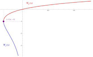
Figure 1: The two real branches of $W(x)$.

The derivative of $W(z)$ reads

$$\frac{dW(z)}{dz}=\frac{W(z)}{z(1+W(z))},~{}~{}\forall z\notin\left\{0,-1/e\right\};~{}~{}\frac{dW(z)}{dz}\bigg{|}_{z=0}=1\,,$$ (B.2)

and is not defined for $z=-1/e$ (the function is not differentiable there). At that point we have

$$\lim_{x\rightarrow-1/e}\frac{dW_{0}(x)}{dx}=\infty,~{}~{}\lim_{x\rightarrow-1/e}\frac{dW_{-1}(x)}{dx}=-\infty\,.$$ (B.3)

Instituto de Física Teórica UAM/CSIC,
C/ Nicolás Cabrera, 13-15, C.U. Cantoblanco, 28049 Madrid, Spain

IFT Number: IFT-UAM/CSIC-13-054

E-mail:
${\color[rgb]{1,0,0}\varheart}$pab.bueno[at]estudiante.uam.es
${\color[rgb]{0.55,0.14,1}\varheart}$carlos.shabazi[at]uam.es

References

- [1] A. Strominger and C. Vafa, Microscopic origin of the Bekenstein-Hawking entropy, Phys.Lett. B379 (1996) 99–104, [hep-th/9601029].
- [2] A. Sen, Black Hole Entropy Function, Attractors and Precision Counting of Microstates, Gen.Rel.Grav. 40 (2008) 2249–2431, [arXiv:0708.1270].
- [3] I. Mandal and A. Sen, Black Hole Microstate Counting and its Macroscopic Counterpart, Nucl.Phys.Proc.Suppl. 216 (2011) 147–168, [arXiv:1008.3801].
- [4] G. Lopes Cardoso, B. de Wit, and T. Mohaupt, Corrections to macroscopic supersymmetric black hole entropy, Phys.Lett. B451 (1999) 309–316, [hep-th/9812082].
- [5] G. Lopes Cardoso, B. de Wit, and T. Mohaupt, Macroscopic entropy formulae and nonholomorphic corrections for supersymmetric black holes, Nucl.Phys. B567 (2000) 87–110, [hep-th/9906094].
- [6] G. Lopes Cardoso, B. de Wit, J. Kappeli, and T. Mohaupt, Stationary BPS solutions in N=2 supergravity with R**2 interactions, JHEP 0012 (2000) 019, [hep-th/0009234].
- [7] T. Mohaupt, Black hole entropy, special geometry and strings, Fortsch.Phys. 49 (2001) 3–161, [hep-th/0007195].
- [8] A. Dabholkar, R. Kallosh, and A. Maloney, A Stringy cloak for a classical singularity, JHEP 0412 (2004) 059, [hep-th/0410076].
- [9] P. Candelas, X. C. De la Ossa, P. S. Green, and L. Parkes, An Exactly soluble superconformal theory from a mirror pair of Calabi-Yau manifolds, Phys.Lett. B258 (1991) 118–126.
- [10] P. Candelas, X. C. De La Ossa, P. S. Green, and L. Parkes, A Pair of Calabi-Yau manifolds as an exactly soluble superconformal theory, Nucl.Phys. B359 (1991) 21–74.
- [11] S. Hosono, A. Klemm, S. Theisen, and S.-T. Yau, Mirror symmetry, mirror map and applications to Calabi-Yau hypersurfaces, Commun.Math.Phys. 167 (1995) 301–350, [hep-th/9308122].
- [12] S. Hosono, A. Klemm, and S. Theisen, Lectures on mirror symmetry, hep-th/9403096.
- [13] K. Behrndt, G. Lopes Cardoso, and I. Gaida, Quantum N=2 supersymmetric black holes in the S-T model, Nucl.Phys. B506 (1997) 267–292, [hep-th/9704095].
- [14] I. Gaida, Gauge symmetry enhancement and N=2 supersymmetric quantum black holes in heterotic string vacua, Nucl.Phys. B514 (1998) 227–241, [hep-th/9705150].
- [15] K. Behrndt and I. Gaida, Subleading contributions from instanton corrections in N=2 supersymmetric black hole entropy, Phys.Lett. B401 (1997) 263–267, [hep-th/9702168].
- [16] I. Gaida, N=2 supersymmetric quantum black holes in five-dimensional heterotic string vacua, Phys.Lett. B429 (1998) 297–303, [hep-th/9802140].
- [17] P. Galli, T. Ortin, J. Perz, and C. S. Shahbazi, Black hole solutions of N=2, d=4 supergravity with a quantum correction, in the H-FGK formalism, arXiv:1212.0303.
- [18] S. Bellucci, S. Ferrara, A. Marrani, and A. Shcherbakov, Splitting of Attractors in 1-modulus Quantum Corrected Special Geometry, JHEP 0802 (2008) 088, [arXiv:0710.3559].
- [19] S. Bellucci, A. Marrani, and R. Roychowdhury, On Quantum Special Kaehler Geometry, Int.J.Mod.Phys. A25 (2010) 1891–1935, [arXiv:0910.4249].
- [20] P. Bueno, R. Davies, and C. S. Shahbazi, Quantum Black Holes in Type-IIA String Theory, JHEP 1301 (2013) 089, [arXiv:1210.2817].
- [21] T. Mohaupt and O. Vaughan, Non-extremal Black Holes, Harmonic Functions, and Attractor Equations, Class.Quant.Grav. 27 (2010) 235008, [arXiv:1006.3439].
- [22] T. Mohaupt and O. Vaughan, The Hesse potential, the c-map and black hole solutions, JHEP 1207 (2012) 163, [arXiv:1112.2876].
- [23] P. Galli, T. Ortin, J. Perz, and C. S. Shahbazi, Non-extremal black holes of N=2, d=4 supergravity, JHEP 1107 (2011) 041, [arXiv:1105.3311].
- [24] P. Meessen, T. Ortin, J. Perz, and C. S. Shahbazi, H-FGK formalism for black-hole solutions of N=2, d=4 and d=5 supergravity, Phys.Lett. B709 (2012) 260–265, [arXiv:1112.3332].
- [25] P. Meessen, T. Ortin, J. Perz, and C. S. Shahbazi, Black holes and black strings of N=2, d=5 supergravity in the H-FGK formalism, JHEP 1209 (2012) 001, [arXiv:1204.0507].
- [26] P. Galli, P. Meessen, and T. Ortin, The Freudenthal gauge symmetry of the black holes of N=2,d=4 supergravity, arXiv:1211.7296.
- [27] J. H. Lambert, Observationes variae in mathesin puram, Acta Helveticae physico-mathematico-anatomico-botanico-medica (1758) 128, 168.
- [28] P. Bueno, T. Ortín, and C. S. Shahbazi, In preparation, -.
- [29] P. Galli, K. Goldstein, and J. Perz, On anharmonic stabilisation equations for black holes, JHEP 1303 (2013) 036, [arXiv:1211.7295].
- [30] K. Hristov, S. Katmadas, and V. Pozzoli, Ungauging black holes and hidden supercharges, JHEP 1301 (2013) 110, [arXiv:1211.0035].
- [31] F. Denef and G. W. Moore, Split states, entropy enigmas, holes and halos, JHEP 1111 (2011) 129, [hep-th/0702146].
- [32] S. L. Cacciatori, A. Marrani, and B. van Geemen, Multi-Centered Invariants, Plethysm and Grassmannians, JHEP 1302 (2013) 049, [arXiv:1211.3432].
- [33] S. Ferrara, A. Marrani, A. Shcherbakov, and A. Yeranyan, Multi-Centered First Order Formalism, JHEP 1305 (2013) 127, [arXiv:1211.3262].
- [34] S. Ferrara and A. Marrani, On Symmetries of Extremal Black Holes with One and Two Centers, arXiv:1207.7016.
- [35] L. Andrianopoli, R. D’Auria, S. Ferrara, A. Marrani, and M. Trigiante, Two-Centered Magical Charge Orbits, JHEP 1104 (2011) 041, [arXiv:1101.3496].
- [36] S. Ferrara, A. Marrani, E. Orazi, R. Stora, and A. Yeranyan, Two-Center Black Holes Duality-Invariants for stu Model and its lower-rank Descendants, J.Math.Phys. 52 (2011) 062302, [arXiv:1011.5864].
- [37] F. Denef, Supergravity flows and D-brane stability, JHEP 0008 (2000) 050, [hep-th/0005049].
- [38] B. Bates and F. Denef, Exact solutions for supersymmetric stationary black hole composites, JHEP 1111 (2011) 127, [hep-th/0304094].
- [39] K. Goldstein and S. Katmadas, Almost BPS black holes, JHEP 0905 (2009) 058, [arXiv:0812.4183].
- [40] I. Bena, S. Giusto, C. Ruef, and N. P. Warner, Multi-Center non-BPS Black Holes: the Solution, JHEP 0911 (2009) 032, [arXiv:0908.2121].
- [41] G. Bossard and C. Ruef, Interacting non-BPS black holes, Gen.Rel.Grav. 44 (2012) 21–66, [arXiv:1106.5806].
- [42] V. Jejjala, O. Madden, S. F. Ross, and G. Titchener, Non-supersymmetric smooth geometries and D1-D5-P bound states, Phys.Rev. D71 (2005) 124030, [hep-th/0504181].
- [43] I. Bena, S. Giusto, C. Ruef, and N. P. Warner, A (Running) Bolt for New Reasons, JHEP 0911 (2009) 089, [arXiv:0909.2559].
- [44] N. Bobev and C. Ruef, The Nuts and Bolts of Einstein-Maxwell Solutions, JHEP 1001 (2010) 124, [arXiv:0912.0010].
- [45] P. Candelas and X. de la Ossa, Moduli space of Calabi-Yau manifolds, Nucl.Phys. B355 (1991) 455–481.
- [46] C. Shahbazi, Black Holes in Supergravity with Applications to String Theory, arXiv:1307.3064.
- [47] S. Ferrara, G. W. Gibbons, and R. Kallosh, Black holes and critical points in moduli space, Nucl.Phys. B500 (1997) 75–93, [hep-th/9702103].
- [48] S. Sorgato, Black Holes and Taub-NUT spacetimes in N=2 Supergravity. M.Sc. Thesis, .
- [49] L. Andrianopoli, M. Bertolini, A. Ceresole, R. D’Auria, S. Ferrara, et al., N=2 supergravity and N=2 superYang-Mills theory on general scalar manifolds: Symplectic covariance, gaugings and the momentum map, J.Geom.Phys. 23 (1997) 111–189, [hep-th/9605032].
- [50] K. Tod, All Metrics Admitting Supercovariantly Constant Spinors, Phys.Lett. B121 (1983) 241–244.
- [51] K. Behrndt, D. Lust, and W. A. Sabra, Stationary solutions of N=2 supergravity, Nucl.Phys. B510 (1998) 264–288, [hep-th/9705169].
- [52] P. Meessen and T. Ortin, The Supersymmetric configurations of N=2, D=4 supergravity coupled to vector supermultiplets, Nucl.Phys. B749 (2006) 291–324, [hep-th/0603099].
- [53] L. Lewin, Polylogarithms and Associated Functions. North-Holland, Amsterdam, 1981.
- [54] R. M. Corless, D. J. Jeffrey, and S. R. Valluri, Some Applications of the Lambert W Function to Physics, Can. J. Phys.78 (2000) 823, 831.
- [55] J. M. Caillol, Some applications of the Lambert W function to classical statistical mechanics, Journal of Physics A Mathematical General 36 (Oct., 2003) 10431–10442, [cond-mat/0306562].
- [56] E. Gardi, G. Grunberg, and M. Karliner, Can the QCD running coupling have a causal analyticity structure?, JHEP 9807 (1998) 007, [hep-ph/9806462].
- [57] B. Magradze, The Gluon propagator in analytic perturbation theory, Conf.Proc. C980518 (1999) 158–169, [hep-ph/9808247].
- [58] A. Nesterenko, Analytic invariant charge in QCD, Int.J.Mod.Phys. A18 (2003) 5475–5520, [hep-ph/0308288].
- [59] G. Cvetic and I. Kondrashuk, Explicit solutions for effective four- and five-loop QCD running coupling, JHEP 1112 (2011) 019, [arXiv:1110.2545].
- [60] H. Sonoda, Solving RG equations with the Lambert W function, arXiv:1302.6069.
- [61] A. Ashoorioon, A. Kempf, and R. B. Mann, Minimum length cutoff in inflation and uniqueness of the action, Phys.Rev. D71 (2005) 023503, [astro-ph/0410139].
- [62] T. C. Scott and R. B. Mann, General Relativity and Quantum Mechanics: Towards a Generalization of the Lambert W Function, ArXiv Mathematical Physics e-prints (July, 2006) [math-ph/0607011].
- [63] R. B. Mann and T. Ohta, Exact solution for the metric and the motion of two bodies in (1+1)-dimensional gravity, Phys.Rev. D55 (1997) 4723–4747, [gr-qc/9611008].