Exploration of stable and unstable vortex patterns in a superconductor under a magnetic disc

Abstract

The stable and unstable solutions of a square 2D extreme type-II superconductor are studied in the field of a magnetic disc. We use a preconditioned Newton-Krylov solver to find the solutions and use numerical continuation to track the solutions as the field strength varies. For a disc with a small radius, we have identified generic scenarios through which the state loses and regains its stability.

I Introduction

Mesoscopic phenomena have been at the forefront of research in superconductivity in the last 15 years.Grigorieva et al. (1997); Moshchalkov et al. (1995); Schweigert et al. (1998); Baelus and Peeters (2002); Kanda et al. (2004); Mel’nikov and Vinokur (2002) The key property of mesoscopic samples is the strong influence of confinement on the superconducting condensate, and subsequent quantum tailoring of superconductivity. There it is particularly important that critical parameters can be enhanced by confinement. For example, critical magnetic field of mesoscopic superconductors can be multiply larger than one of bulk materials. In addition, since the size of a mesoscopic sample is comparable to the scale of the vortex-vortex interaction, there is a strong influence of the boundary on the flux distribution in the sample (i.e. vortex configurations). Additional influence on the aforementioned phenomena can be made by nanoengineering, e.g. by introducing holes in the sample Baelus et al. (2000); Xu et al. (2008), or magnets embedded in, or placed on top of the superconductor Milošević et al. (2007). Namely, the strongly inhomogeneous magnetic field of the ferromagnet interacts with externally applied magnetic field and changes the magnetic environment for the superconductor, while also altering the spatial domain for emerging vortices and stimulating nucleation of vortex-antivortex pairs.

The subject of superconductor-ferromagnet hybrids is very mature, and several reviews are available Velez et al. (2008); Lyuksyutov* and Pokrovsky (2005); Aladyshkin et al. (2009). However, the literature to date has studied mainly the stable vortex(-antivortex) configurations and how they depend on the parameters of the system such as field strength or geometry. Virtually nothing is known about how these states behave when they lose their stability and how the transitions between stable states occur, i.e. how vortices nucleate or enter the system, and how the energy barriers for those processes can be quantified. Understanding this is clearly important for any emerging devices that control or exploit the behavior of the vortices Milosevic and Peeters (2010).

To arrive at a complete picture it is thus necessary to know the location and evolution of the unstable or so-called saddle-point states. Such states and their free energies directly determine the possible transitions and the height of the energy barrier that separate the stable states. An approach to study the saddle points has been proposed in Ref. Schweigert and Peeters (1999) and utilized in Ref. Baelus et al. (2001), but only for 2D superconducting disks. The radial symmetry of the sample was crucial for the efficiency of the approach, although theoretical formalism is generally applicable once the eigenfuctions of the linearized Ginzburg-Landau equation are known for the chosen geometry.

One more reason to study the saddle points in detail is the fact that knowledge about the unstable states and their bifurcations together with the symmetries of the system allows to analyze superconductors by tools of the mathematics of dynamical systems. One can then use the known techniques from pattern formation,Hoyle (2006) which would further expand the scientific community and cross-fertilization of different subjects and fields of study.

Therefore, in this paper we demonstrate the use of a new high-performance solver for both stable and unstable solutions of the Ginzburg-Landau equation, for an arbitrary superconducting geometry, and in presence of an arbitrary magnetic field. As an exemplary case, we choose superconducting square with a magnetic disc on top, with additional possibility of added homogeneous magnetic field. Important part of the presented study is the method of numerical continuation of relevant parameters, which has been successfully used for Bose-Einstein condensates Law et al. (2010); Huepe et al. (2003). The solver we use is proposed in Schlömer and Vanroose (2013) and is available as a open-source library at Schlömer

The outline of the paper is follows. In Sec. II we describe the system, its numerical representation and how the resulting system can be solved using a Newton-Krylov iteration. We then show how to track the solutions as the parameters of the system change in Sec. II.3. In Sec. III we show the stable and unstable solutions, and transitions between them, for a square superconducting domain in external homogeneous field. The results for a hybrid structure are given further, for a small magnetic disc in Sec. 3 and for a large disc in Sec. V. We conclude with a discussion and summary in Sec. VI.

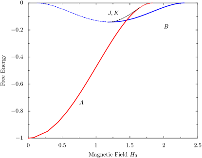
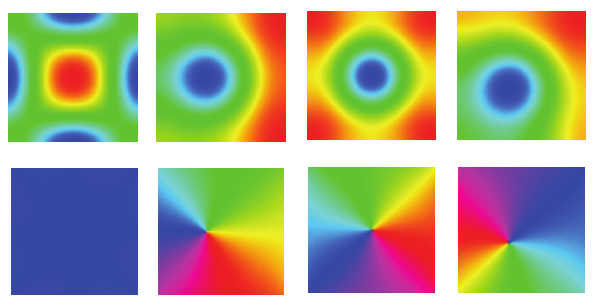
Figure 1: (Color online) The stable and unstable states in a $3\xi\times 3\xi$ superconducting square sample in a homogeneous field. The branch $A$ loses it stability for large fields, while the branch $B$ that has a single vortex in the center of the domain gains stability for large fields. The two bifurcation points are connected through two unstable branches $J$ and $K$. The corresponding patterns are shown below where we show from left to right the pattern for curve $A$, $J$ and $B$ and $K$ respectively. Curve $J$ has a pattern entering along the center line, while curve $K$ has it entering along the diagonal. We refer to Schlömer et al. (2012) for more details.

II The Ginzburg-Landau equation and its numerical solution

II.1 Description of the system

We look at extreme type II superconductors where the magnetic field is not modified by the super-currents that are generated by the superconductor. In this case, the Ginzburg–Landau problem decouples and results in

$$\mathcal{GL}(\psi)=\begin{cases}0=\left(-\textup{i}\bm{\nabla}-\bm{A}\right)^{2}\psi-\psi\left(1-|\psi|^{2}\right)\quad\text{in }\Omega,\\[8.53581pt] 0=\mathbf{n}\cdot(-\textup{i}\bm{\nabla}-\bm{A})\psi\quad\text{on }\partial\Omega,\end{cases}$$ (1)

where $\bm{A}$ is the given magnetic vector potential and $\psi$ is the order parameter describing the superconducting state.

In this paper we study problems where the magnetic field is generated by a magnetic disc. The vector potential is then an integral of the magnetic dipole over the volume $V$ of the disc

$$\bm{A}(\mathbf{x})=\int_{V}\frac{\mathbf{m}\times(\mathbf{x}-\mathbf{z})}{\|\mathbf{x}-\mathbf{z}\|^{3/2}}d\mathbf{z}$$ (2)

where m is the magnetic moment. In this example it is oriented along the $z$-axis.

The magnetic disc has a height $h$ and a radius $r$ and sits a distance $z$ above the center of the square domain.

II.2 Newton–Krylov method

We use a Newton-Krylov iterative method to find the solution of (1). The Newton iteration is an outer iteration that deals with the nonlinearity of the equation where each iteration requires the solution of the Jacobian system. The Krylov subspace method is an inner iteration where the Jacobian system is solved iteratively. The advantage of this method is that the Newton method converges superlinearly in the neighborhood of a steady state, irrespective of the stability properties of the solution. It starts from an initial guess $\psi^{(0)}$ and a sequence of approximations $\psi^{(k+1)}=\psi^{(k)}+\delta\psi^{(k)}$ is generated. The update $\delta\psi^{(k)}$ satisfies the linear system

$$\mathcal{J}(\psi^{(k)})\delta\psi^{(k)}=-\mathcal{GL}(\psi^{(k)}).$$ (3)

The Jacobian $\mathcal{J}$ is a linear operator defined via the action

$$\mathcal{J}(\psi)\phi=(\mathcal{K}+V+2g|\psi|^{2})\phi+g\psi^{2}\overline{\phi},$$ (4)

where $\overline{\phi}$ denotes complex conjugation.

Solving the large linear system (3) in a scalable way is the most significant difficulty when applying Newton’s method to nonlinear Schrödinger equations. However, the linear systems such as (3) can be solved using Krylov iterative methods that do not require an explicit (matrix) representation of the operator but only its application to vectors such as (4). The convergence of those methods is highly dependent on the spectrum of the involved linear operator.

To solve the Jacobian system, we use the method proposed in Schlömer and Vanroose (2013) where it is shown that $\mathcal{J}$ from Eq. (4) associated with the nonlinear Schrödinger equations is self-adjoint with respect to the inner product

$$\langle\phi,\psi\rangle\mathrel{\mathop{:}}=\Re\left(\int_{\Omega}\overline{\phi}\psi\right).$$ (5)

The paper suggests to use MINRES Greenbaum (1997), a Krylov subspace method suitable for indefinite self-adjoint problems.

One characteristic of Krylov methods is that a larger number of unknowns increases the number of iterations that are needed to achieve convergence. In addition, the computational cost of a single evaluation of the linear action also grows with the number of unknowns. Therefore, high-resolution discretizations of three-dimensional systems would require a significant computational effort.

In Schlömer and Vanroose (2013) a preconditioner is proposed for the linear problem. The main idea is that, instead of solving the discretized version $Jx=b$ of (3), one can solve an equivalent, numerically more favorable problem $P^{-1}Jx=P^{-1}b$ with a linear, invertible preconditioning operator $P$. If $P$ is appropriately chosen, Krylov methods applied to the new system converge much faster. In the case of the linearization of nonlinear Schrödinger operators (4), the energy operator $\mathcal{K}$ is of particular interest, as it typically dominates the spectral behavior of $\mathcal{J}(\psi)$. More precisely, define the symmetric preconditioning operator

$$\mathcal{P}(\psi)\mathrel{\mathop{:}}=\mathcal{K}+2\max\{g,\varepsilon\}|\psi|^{2},$$ (6)

with $0<\varepsilon\ll 1$ Schlömer and Vanroose (2013). Note that $\mathcal{P}(\psi)$ is strictly positive-definite except for the uninteresting case of $\psi\equiv 0$. This, most importantly, makes the inversion of the discretized $\mathcal{P}(\psi)$, $P^{-1}(\psi)$, computationally cheap since its positive-definiteness makes it a suitable target for geometric or algebraic multigrid (AMG) solvers that yield optimal convergence Trottenberg et al. (2001). As will be shown, even inexact inversions of (6) used as preconditioners for (4) make the Krylov convergence independent of the number of unknowns.

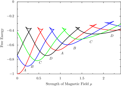
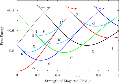
Figure 2: (Color online) Top: over view of the states of a $10\xi\times 10\xi$ superconducting sample under a magnetic disc of radius $r=2\xi$. The curve $A$, $B$, $C$ and $D$ have full symmetry of the system and they form swallow tails where stability is lost and regained. Bottom: Detail for weak fields. Solid curves are stable and dotted curves are unstable. Representative patterns along each of these curves are shown in Fig. 3. Between the bifurcation points, labeled as 1, 2, 3, …, there are connecting curves with patterns with a reduced symmetry. The curves $E$, $F$, $G$ and $H$ are unstable and have an additional vortex of multiple vortices moving in along one of the center lines. Representative patterns for these curves are shown in Fig. 4

II.3 Numerical Continuation

The efficient linear solver from Schlömer and Vanroose (2013) can be combined with numerical parameter continuation into an efficient method for the exploration of the energy landscape. Numerical parameter continuation is a well-established technique for numerical bifurcation analysis of dynamical systems Keller et al. (1987); Krauskopf (2007). It extends the non-linear system to include parameters like the magnetic field strength. A function $F:\mathbb{C}^{N}\times\mathbb{R}\rightarrow\mathbb{C}^{N}$ is considered that maps $\mathbf{x}:=(\psi,\mu)$, a combination of the numerical representation of $\psi$ and the parameter $\mu$ of the magnetic field, to zero:

$$F(\mathbf{x})=0$$ (7)

By the implicit function theorem, this defines a family of solutions $\psi(\mu)$ that can be generated numerically.

Numerical continuation follows a predictor-corrector scheme to construct, starting from an initial solution point $\mathbf{x}_{0}=(\psi_{0},\mu_{0})$, the successive points on the solution curve. The predictor step is an Euler predictor that uses the unit length tangent vector $\mathbf{t}_{i}$ to the curve at a solution point $\mathbf{x}_{i}$ that satisfies $F(\mathbf{x}_{i})=0$ and a step size $s>0$ to predict a guess $\mathbf{x}^{\text{P}}_{i+1}$ for the next point on the curve

$$\mathbf{x}_{i+1}^{\text{P}}=\mathbf{x}_{i}+s\mathbf{t}_{i}.$$ (8)

The corrector step improves the guess $\mathbf{x}^{\text{P}}_{i+1}$ with a Newton iteration on the augmented system to obtain a new solution point $\mathbf{x}_{i+1}$. This augmented system has, in addition to the constraint that $F(\mathbf{x}_{i+1})=0$, the requirement that $\mathbf{x}_{i+1}$ must lie on the hyper-plane through $\mathbf{x}^{\text{P}}_{i+1}$ perpendicular to $\mathbf{t}_{i}$ , the tangent to the previous solution. This translates into the system

$$\begin{cases}F(\mathbf{x}_{i+1})=0\\ (\mathbf{x}_{i+1}-\mathbf{x}^{\text{P}}_{i+1})^{\text{T}}\cdot\mathbf{t}_{i}=0,\end{cases}$$ (9)

where $\cdot$ is the dot-product and $T$ denotes the transpose. This system is a map from $\mathbb{C}^{n}\times\mathbb{R}$ to $\mathbb{C}^{n}\times\mathbb{R}$ and defines, under some conditions that are usually met, uniquely the next point on the solution curve Krauskopf (2007).

The system is solved again with a Newton-Krylov procedure. The Jacobians of this augmented system is very similar to the Jacobian of the Ginzburg-Landau equation. It is only extended with one row and column. The column contains the derivatives of the system to the parameters. The additional row depends on the tangent that appears in the system (9). Again the system can be solved with a Newton-Krylov iteration.

Repeated application of a continuation step makes it possible to follow a solution of the Ginzburg-Landau equation as the strength of the magnetic field changes. Since Newton iterations are insensitive to the states’ stability properties we are able to track the state even when the stability changes and its transitions from stable to unstable.

III Homogeneous Field

For a square system in a homogeneous field a systematic analysis of the stable and unstable patterns has been performed in Schlömer et al. (2012). The paper shows how the patterns change as the strength of the applied field changed. Especially the transitions between stable and unstable states have been studied in detail.

We reproduce in Figure 1 the results for a small domain with edge length $d=3\xi$. This system is so small that it only supports a few vortices. The figure shows the free energy as a function of the strength of the homogeneous magnetic field. The curve $A$ starts at $\mu=0$ where the system is in the homogeneous solution $\psi\equiv 1$ and is completely superconducting. The solution has all the symmetries of the system and is stable as a global minimum of the free energy.

For nonzero field strength, the solutions deviate from the homogeneous superconducting state, developing zones of lower supercurrents near the edges of the domain. At field strength $\mu\approx 1.64$, an eigenvalue with multiplicity 2 becomes unstable.

At this bifurcation point two different families of solution branches emerge. Both are unstable and correspond to a single vortex moving towards the middle of the domain. Along branch $J$ a single vortex moves towards the center along one of the center lines. Along branch $K$ a single vortex moves along one of the diagonals.

Both connect with branch $B$ in the other bifurcation point. This branch has one vortex in the middle of the domain but it is unstable for small magnetic fields. It becomes stable at the second bifurcation point and it remains stable until the superconductivity is lost for large field strengths.

The two curves $J$ and $K$ that connect the two bifurcation points correspond to maxima in the free energy curve while the solid curves correspond to minima. In that light the calculation of these unstable states and their corresponding energy is valuable since it gives an indication of the energy that is required to cross the barrier between two stable states for a fixed magnetic field. Indeed, a transition between the stable state without vortices and the stable state with a vortex would require a transition where a vortex enters the domain. The energy of this state is given in Fig. 1.

For larger systems in a homogeneous field similar bifurcation diagrams can be constructed and there are many connections between the bifurcation points. We refer to Schlömer et al. (2012) for a complete discussion of the stable and unstable states of a square system in a homogeneous field.

IV Square domain under a disc with radius $2\xi$

Curve $A$

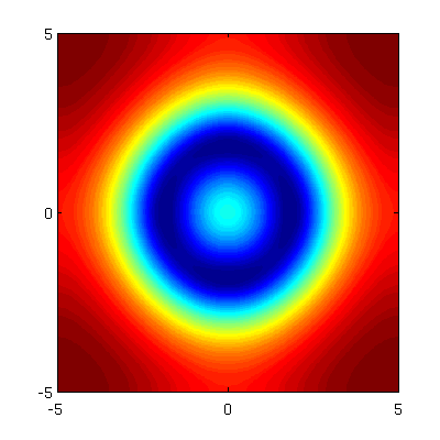
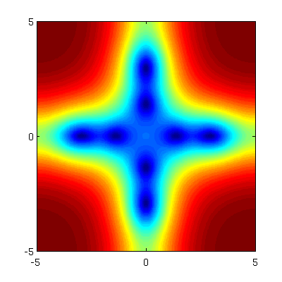
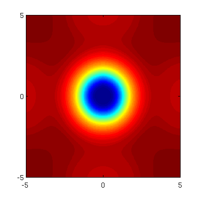
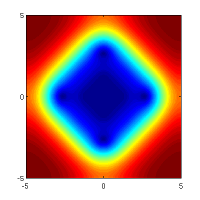
Curve $B$

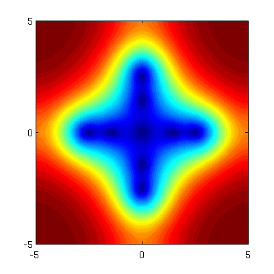
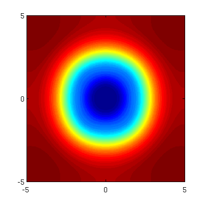
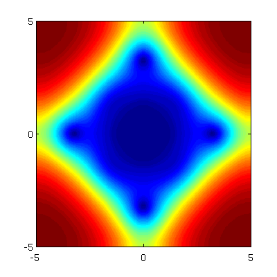
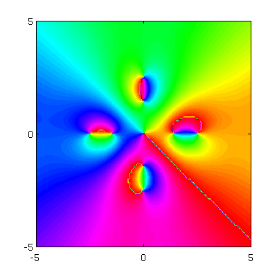
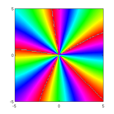
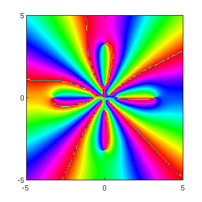
Curve $C$

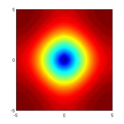
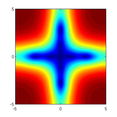
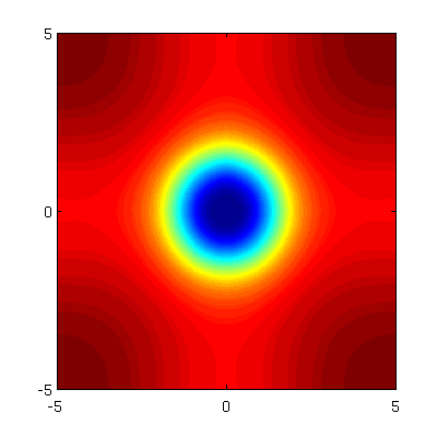
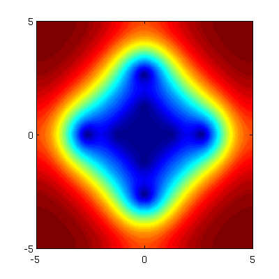
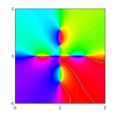
Curve $D$

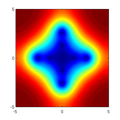
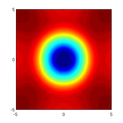
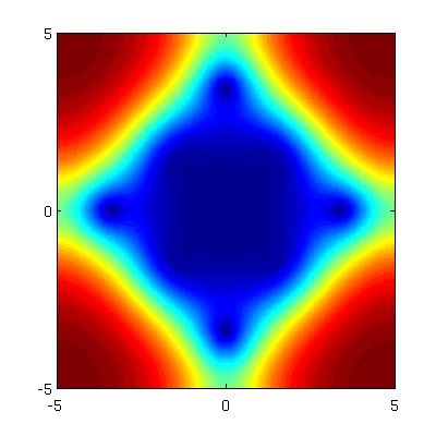
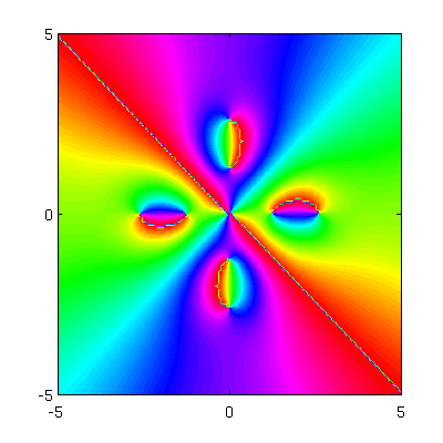
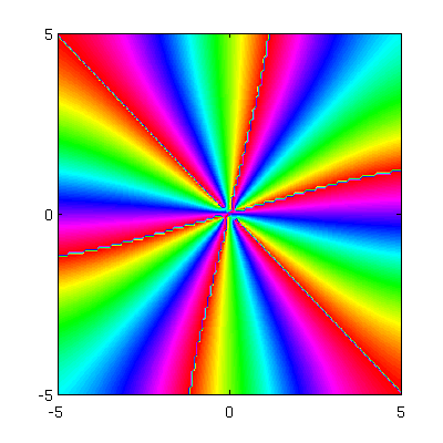
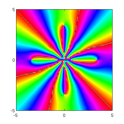
Figure 3: (Color online) The patterns that are formed for a system with a magnetic disc of radius $r=2\xi$. We show the representative patterns along curve $A$, $B$, $C$ and $D$ for increasing magnetic field strength. Each of the curves go through the same sequence. Under the edge of the magnetic disc four pairs of vortex and anti-vortex are formed. As the field increases further the four anti-vortices move out of the system and the four remaining vortices merge with the vortex that is already present in the middle to form a giant vortex. Along this sequence the multiplicity is increased with four. Then as the field increases further additional pairs of vortices and anti-vertices merge.

In this section we look at a thin square superconducting domain with size $10\xi\times 10\xi$. It sits under a superconducting disc of of height $1\xi$ and radius of $2\xi$. It sits a distance $0.1\xi$ above the superconducting sample.

In Fig. 2 we show the free energy of the states that appear in the system as a function of the magnetic field. Initially we discuss the states that have all the symmetries of the square domain, i.e the symmetry group $D_{4}$ (see Schlömer et al. (2012)). There are four curves with full symmetry denoted with labels $A$, $B$, $C$ and $D$. The stability of the states along these curves changes in bifurcation points denoted with $1$, $2$, $3$, $\ldots$. The curves $E$, $F$, $G$ and $H$ are connecting curves that connect bifurcation points on different curves.

IV.0.1 Curve $A$

Let us start with curve $A$. It starts at the trivial state $\psi\equiv 1$ at zero magnetic field. As the field increases the free energy of the curve rises and the solution starts to deviate from the trivial solution. Especially under the edge of the magnetic disc the superconductivity is perturbed by the steep changes in the magnetic field.

The curve $A$ becomes unstable at $\mu=0.446$ in the bifurcation point 1. Here an eigenvalue of the Jacobian becomes positive real and the system becomes unstable. At this bifurcation point the curve $E$ connects to the branch to curve $B$. This saddle point curve is unstable and has a single vortex solution. The connecting curves will be discussed later in detail in Sec. IV.0.2.

On curve $A$, next to bifurcation point 1, there is a second bifurcation point 2 with a slightly increased strength of the magnetic field where a second eigenvalue becomes positive real. This second bifurcation point connects through curve $F$, a branch that features two vortices moving in, to branch $C$. Again, this curve will be discussed later.

At fields around $\mu=0.591$ on curve $A$ the perturbations under the edge of the magnetic disc become more pronounced and four vortex-anti-vortex pairs are formed. These vortex-anti-vortex pairs form where the center lines of the square intersect with the circle of the edge of the magnetic disc. This is where the edge of the magnetic disc is closest to the edges of the square domain. The formation of these pairs is shown in the top row of Fig. 3 where representative patterns as shown along curve $A$ as the strength of the magnetic field increases.

As the field increases further, the anti-vortex and the vortex in each pair move apart. The anti-vortex moves along the center line of the square away from the center and towards the edge of the domain and, finally, it moves out of the sample. During this sequence the free energy curve goes through two turning points and the curve forms a swallow tail as can be seen in Fig. 2.

At the same time, as the anti-vortices move out, the four remaining vortices move towards the center of the domain where they merge into a giant vortex of multiplicity four. Such a giant vortex is also shown as one of the patterns for curve $A$ in Fig. 3.

The curve $A$ regains stability at a field strength of $\mu=0.571$ in bifurcation point 3. The solution is now a giant vortex with multiplicity 4. And for the interval $0.895~{}\leq~{}\mu~{}\leq~{}1.175$ the state has the smallest free energy of all states.

The curve remains stable up to field strengths $\mu=1.754$ where it becomes unstable. The curve again forms a swallow tail along which four additional vortex anti-vortex pairs are formed while the giant vortex with multiplicity 4 remains in the center of the system. Again, the anti-vortices move out and the vortices merge with the giant vortex. It has a multiplicity 8.

So at each transition through a swallow tail the multiplicity of the giant vortex is increased by four. Along the curve $A$ we can identify regions of the magnetic field where a stable giant vortex is formed with multiplicity either $4$, $8$, $12$ and so on.

IV.0.2 Curve $B$, $C$ and $D$

The curve $B$ goes through a similar series of transitions as curve $A$. The curve $B$ has for small magnetic fields a single vortex in the middle of the domain. The states have all the symmetries of the system. Similarly to the curve $A$, as the field increases, the free energy curve forms swallow tails where four vortex-anti-vortex pairs are created and split into four vortices that merge with the vortex already present in the center of the domain to form a giant vortex of multiplicity 5. The four anti-vortices move out of the domain along the center lines. This sequence is illustrated in Fig. 3.

So, along the curve $B$ we can identify regions of the magnetic field where a stable giant vortex is formed in the center of the domain with a multiplicity of, subsequently, 1, 5, 9, and so on. Near the bottoms of the free energy curves the states are stable, near the swallow tails they are unstable. At every bifurcation point, where the state transitions from stable to unstable, there are other connecting curves, similar as in curve $A$.

The curve $C$, similar to curve $A$ and $B$, has intervals in the magnetic field strength where stable giant vortices with multiplicity 2, 6, 10, 14, …are formed. These regions are separated by swallow tails similar to those found along the curves $A$ and $B$. Note that the curve $C$ is closely related to curve $B$. Indeed, if we continue curve $B$ in the negative $\mu$ direction we would find the curve $C$ reflected over the $y$-axis.

Also curve $D$ forms the sequence with giant vortices of multiplicity $3$, $7$, $11$, … and shows similar swallow tails as the curves $A$, $B$ and $C$.

The subsequent minima of the free energy form a repeating sequence, as can be seen in the Fig. 2. First, the curve $A$ forms the minimum. For $\mu$ between 0.25 and 0.45 curve $B$ has the minimal energy. Then curve $C$ and $D$ has the state with the minimal energy. Then it is the turn again to curve $A$ to form the pattern with the minimal energy.

IV.1 Connecting saddle point curves

Curve $E$

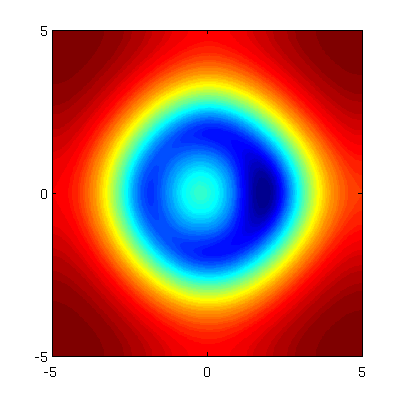
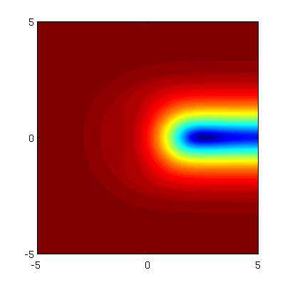
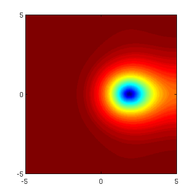
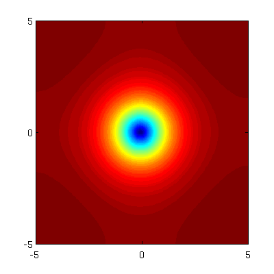
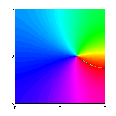
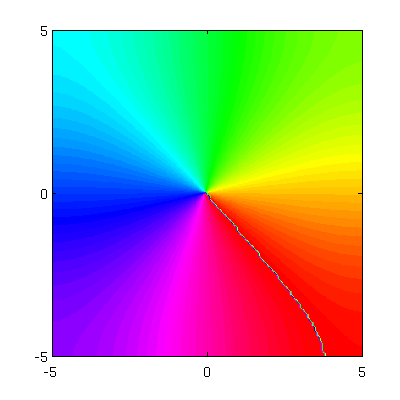
Curve $F$

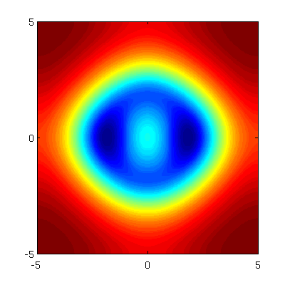
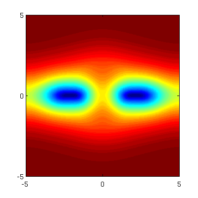
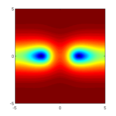
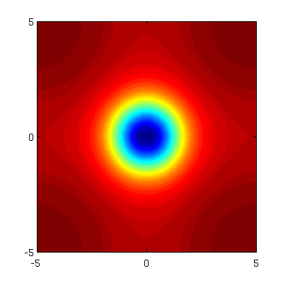
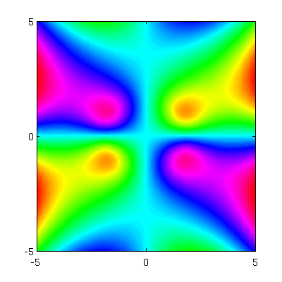
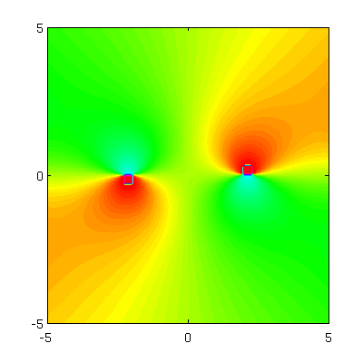
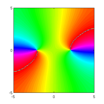
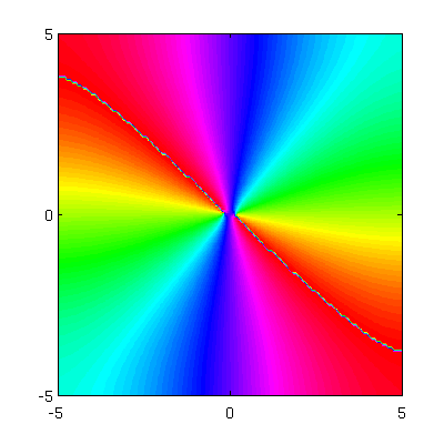
Curve $G$

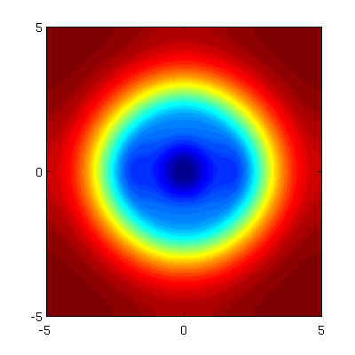
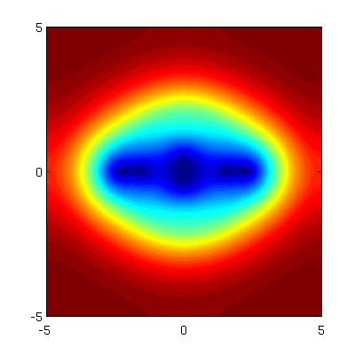
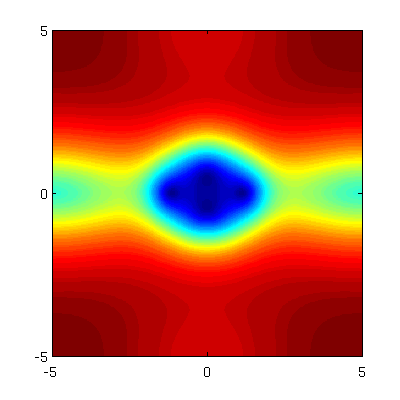
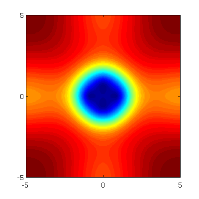
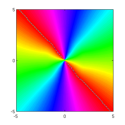
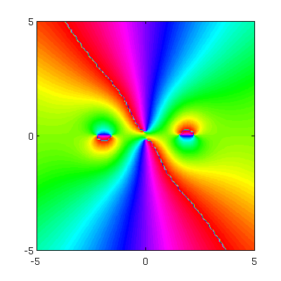
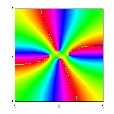
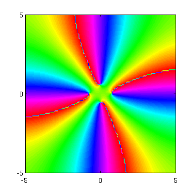
Curve $H$

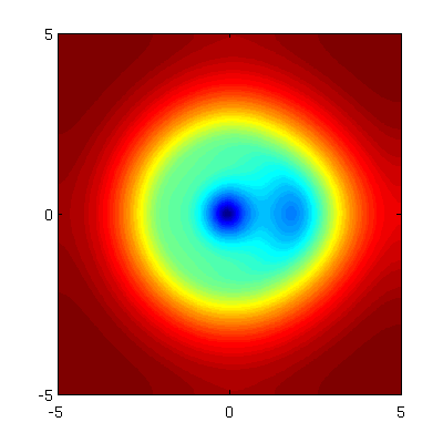
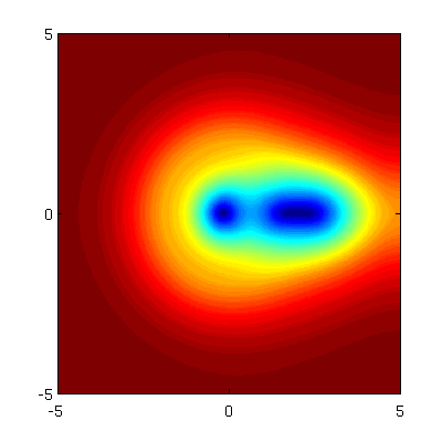
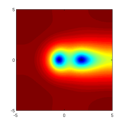
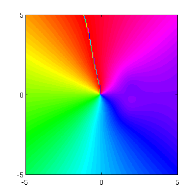
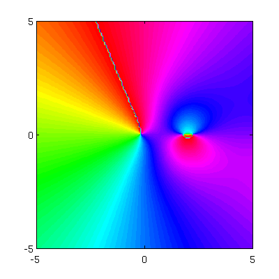
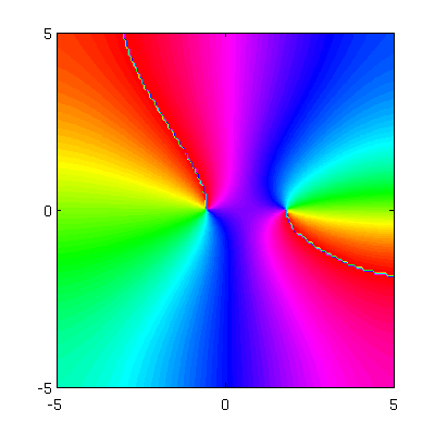
Figure 4: (Color online) The patterns along the connecting curves $E$, $F$, $G$ and $H$ for a magnetic disc of radius $r=2\xi$. These curve have a reduced symmetry compared to the patterns form Fig. 3

Along each of the curves there are several bifurcation points where the states transition from stable to unstable. At these bifurcation points there is an eigenvalue of the Jacobian that crosses the origin and becomes positive real. It is well known in bifurcation theory that at each bifurcation point there is a connecting branch. For a complete discussion on the bifurcations and the connections we refer to the literature on the equivariant bifurcation lemma and related results. A good introduction can be found in Hoyle (2006).

There are many bifurcations along the curves $A$, $B$, $C$ and $D$ and we will not give a complete picture of all bifurcations. We only focus on a few of the generic connecting curves that appear at the first bifurcation points and the connections between them. Als these curves are unstable.

The curve $E$ connects the bifurcation point 1 on curve $A$ with bifurcation point 6 on curve $B$, a curve with a single vortex in the middle. In bifurcation point 1 on curve $A$, there are no vortices in the domain. but along the curve $E$ a single vortex-anti-vortex pair is formed at one of the intersection points of the centerline and the edge of the magnetic discs. There are four possible positions of this pair. Then when the field is weakened the vortex and anti-vortex move away from each other. The anti-vortex leaves the domain and the remaining vortex moves to the center of the domain where it connects with the bifurcation point 6 on curve $B$. A sequence of patterns along this curve is shown in Fig. 4.

In a similar way there is a curve $F$ that connects the bifurcation point 2 on curve $A$ with the bifurcation point 4 on curve $C$. Along this curve two pairs of vortex/anti-vortex are formed. The two anti-vortices move out and the two vortices merge into a giant vortex in the middle of the domain at point 4.

These same saddle point curves also appear between other curves. For example along curve $G$, which connects $B$ with $C$, a single vortex moves in and merges with the already present vortex in to a giant vortex with multiplicity 2 close to bifurcation 4. This is the equivalent branch as curve $E$ that connects $A$ and $B$.

Similarly, along curve $H$ that connects $C$ with $A$ two vortices move to the center where they merge into a giant vortex with multiplicity 4 at bifurcation point 3 on curve $A$.

Again the free energy information about the unstable connecting saddle node curves is useful for the understand the dynamics of a superconductor. Because it gives an indication of the energies required to make a transition between stable state state for a fixed magnetic field.

V Square domain under a disc with radius $4.5\xi$

Curve $A$

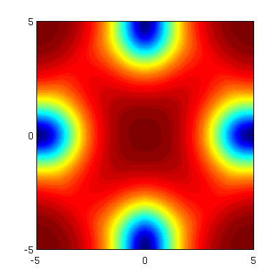
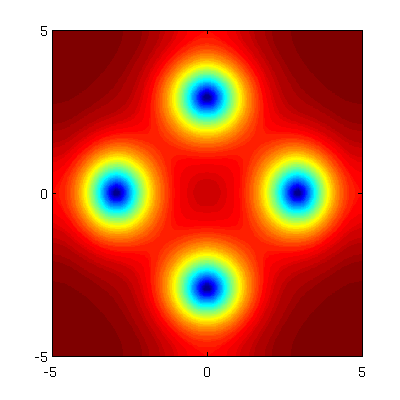
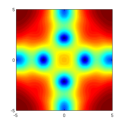
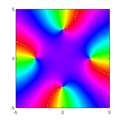
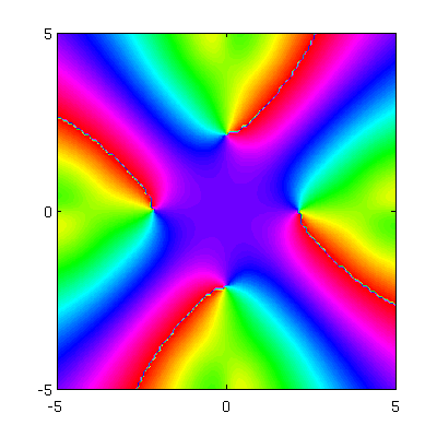
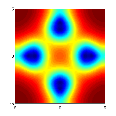
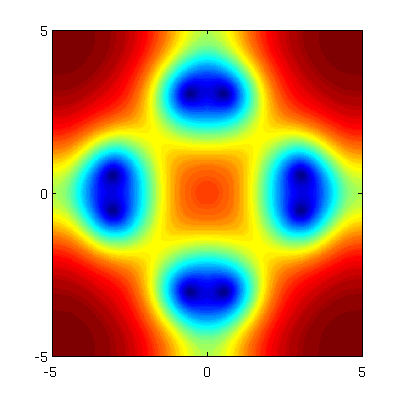
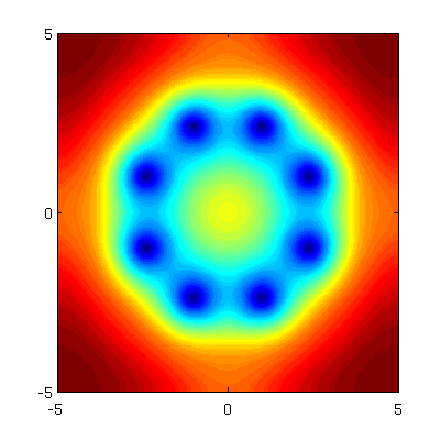
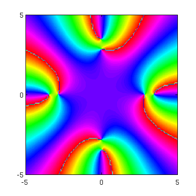
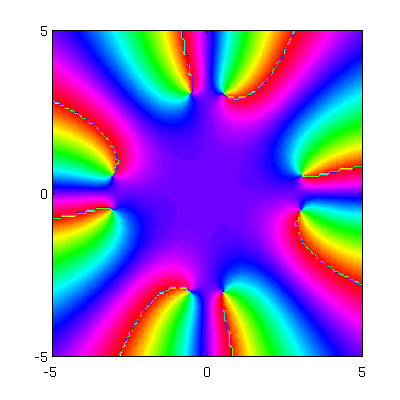
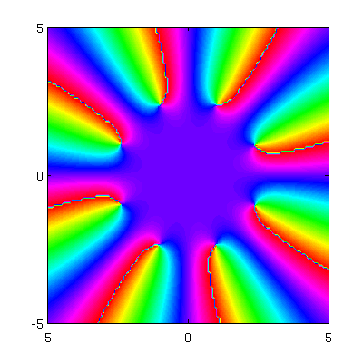
Figure 5: (Color online) The patterns that appear along curve $A$ when the magnetic disc has a radius $r=4.5\xi$, almost equal to the size of the superconducting square. The main difference with the small magnetic disc is that there are no vortices formed in this system. The field strength increases in lexicographic order from top left to bottom right. First four vortices enter along the center lines of the square. However, they never merge into giant vortex in contrast to the small magnetic disc system. These four vortices form a stable pattern. As the field increases further four additional vortices enter the system and they reorganize themselves along a ring. This is also stable for a small range of magnetic fields.

When the magnetic disc is larger, for example, close to the size of the superconducting system, the vortices that appear underneath the magnetic disc do not necessarily have to merge into a giant vortex with a high multiplicity. Indeed, there is enough space under the magnetic disc to support multiple separated vortices. As a result, the transitions between stable and unstable states for a larger system are different from thoses of the previous section. In this section we study a system with a radius of $r=4.5\xi$.

Fig. 7 gives an overview of the branches $A$, $B$, $C$ and $D$ that were discussed earlier in Sec. 3 but are now shown for the larger disc. There are, however, some important differences. Branch $C$ and $D$ are completely unstable and never form a stable configuration of vortices. This in contrast to the system with a small magnetic disc. We will not discuss these patterns in detail.

In Fig 8 and Fig. 5, which shows the corresponding patterns, we follow in detail the branch $A$ that starts from the trivial solution $\psi\equiv 1$ at zero field. Also for this system this state remains stable for small strengths of magnetic field. At a bifurcation point 1 this state loses its stability. Again there is another branch emerging from this bifurcation point. However, now the branch does not connect to a bifurcation point on another branch. Actually, the branch reconnects with the branch $A$ in the bifurcation point $2$, where the branch $A$ regains stability.

In Fig. 5 we follow the pattern along $A$ for the system with radius $4.5\xi$. In contrast to a small system it does not support the formation of vortex anti-vortex pairs. As the field strengthens, four vortices move in along the center lines. This scenario is very similar to what happens in a square superconducting system in a homogeneous magnetic field Schlömer et al. (2012). The four vortices form a stable diamond configuration. As the field strengthens further four additional vortices move in and the eight vortices reorganize themselves in a ring structure underneath the edges of the magnetic disc.

In Fig. 6 we follow the branch $I$ that connects the two bifurcation points on branch $A$ along this branch only two of the four vortices enter the domain. They move to the center as the field increases then two additional vortices enter. The four vortices then reorganize themselves into a diamond shape. At this point it reconnects with the curve $A$.

Curve $I$

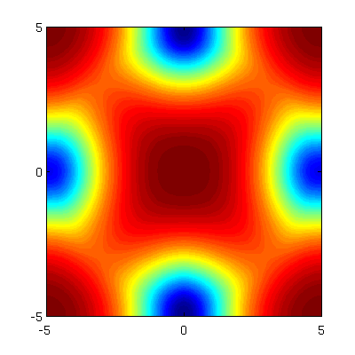
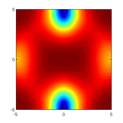
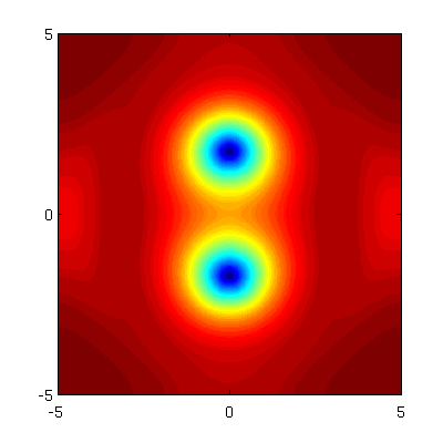
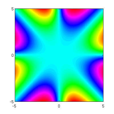
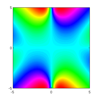
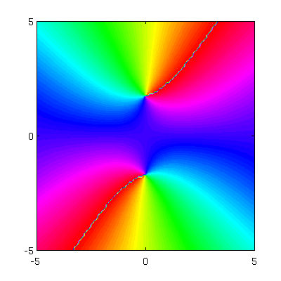
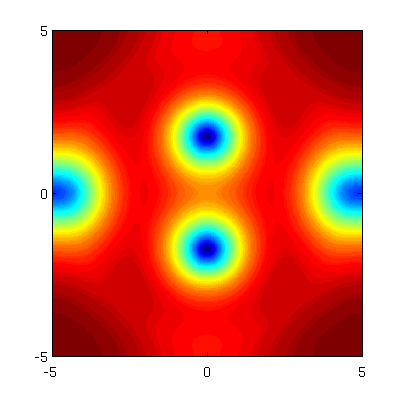
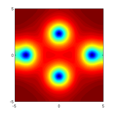
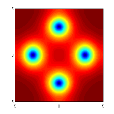
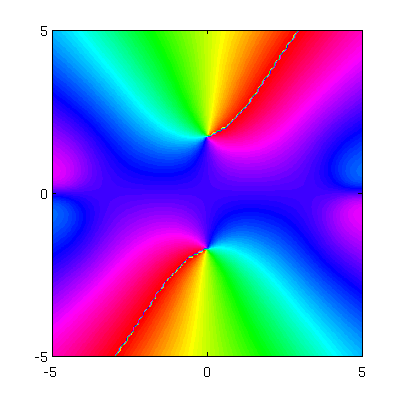
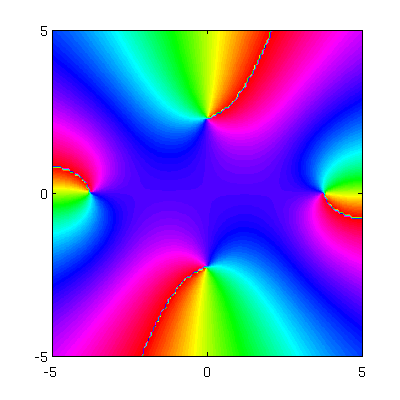
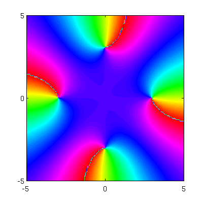
Figure 6: (Color online) The patterns that appear along curve $I$ when the magnetic disc has a radius $r=4.5\xi$

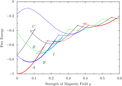
Figure 7: (Color online) Overview of the stable and unstable curves in a $10\xi\times 10\xi$ system under a magnetic disc of radius $4.5\xi$. There are now much shorter stable regions in the curve $A$ and $B$, while the curves $C$ and $D$ are now completely unstable. Further more the connecting curves are now connecting bifurcation points in a different way

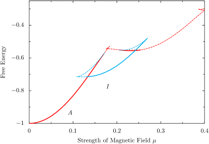
Figure 8: (color online) Detail of Fig. 7. We show how curve $A$ loses and regains its stability at the the swallow tail. At the bifurcation points a connecting curve emerges that has a stable region. This in contrast to the results for the small system

VI Discussion and Conclusions

With the help of a preconditioned Newton-Krylov solver and numerical continuation we have tracked the solutions of the Ginzburg-Landau equations for a thin square extreme type-II superconductor in the field of a magnetic dot. The method is able to track, as a function of the magnetic field, both stable and unstable states. This enables one to study the dynamics of the solutions of the Ginzburg-Landau equations in an arbitrary geometry. The knowledge of the unstable states further gives insight in the possible transitions between stable states and the energy required to cross barriers that separate them.

In this exploration of the free energy landscape we have identified generic scenarios that appear repeatedly in the system. We have studied a square superconductor of size 10$\xi\times$10$\xi$ under a magnetic dot with radius $r=2\xi$ and radius $r=4.5\xi$. In the first system, we have identified a generic scenario that repeats itself over and over as the strength of the magnetic field increases. As a state is tracked as a function of the field strength, the free energy forms a repeating sequence of swallow tails. Along such a swallow tail four pairs of vortex and anti-vortices are formed. The anti-vortices move out of the domain as the field strengthens and the four remaining vortices merge into a giant vortex in the middle of the domain underneath the magnetic dot. This generic scenario repeats itself for subsequent states along their energy curves.

Furthermore, we have identified the saddle point states that connect bifurcations points which appear on the main branches. These branches have reduced symmetry and have one or two vortices moving in the domain. We have not identified all the possible connecting curves, but we expect that there will be connecting saddle point curves with three vortices moving in. Those have been already been observed for samples in a homogeneous field Schlömer et al. (2012).

For the large magnetic dot, with radius $r=4.5\xi$ above scenarios no longer hold because there is enough room underneath the magnetic disc to form separate vortices rather than to collapse into a single giant vortex. At the same time, since the size of the magnet is almost the same as the superconducting domain, the field which the superconductor experiences is practically homogeneous. As a result, the stability properties of the main energy curves are completely changed. Furthermore, the connecting saddle curves form different connections, where appearance of antivortices is scarce.

The obvious continuation of the present work is the extension of the study to 3D systems, based on the efficiency of the solver as shown in Ref. Schlömer et al. (2012). The current work lays the foundation for a systematic bifurcation analysis of vortex rings and loops that may appear around magnetic inclusions in 3D superconductors, as studied in e.g. Ref. Doria et al. (2007). The plethora of there expected stable and unstable states guarantees a promising exploration avenue to follow.