Supplemental material for “Topological order in a correlated Chern insulator”

In this supplemental material, we give further details concerning the $\mathbb{Z}_{2}$ gauge theory description of the interacting Chern insulator [Eq. (4) of the main text], the $K$-matrix description of the intrinsic topological order in the CI* phase, as well as the numerical solution of the slave-particle Hamiltonian for the Haldane-Hubbard model (an example of interacting Chern insulator) in the mean-field approximation.

I Gauge theory representation and saddle-point approximation

While a detailed study of the path integral representation of the $\mathbb{Z}_{2}$ slave-spin theory will appear in a separate publication,z2l here we describe the saddle-point approximation which leads to the final form of the $\mathbb{Z}_{2}$ lattice gauge theory in Eq. (4) of the main text. Following the method described in the Appendix A of Ref. Senthil and Fisher, 2000, one can derive an exact path integral representation of the theory defined by the Hamiltonian (3) of the main text. In order to fully define a theory however, we need to specify not only the Hamiltonian but also the Hilbert space.Wen (2004) The Hamiltonian (3) is written in terms of slave-fermion $f_{r\alpha},f_{r\alpha}^{\dagger}$ and slave-spin $\tau^{x},\tau^{z}$ operators which act on a many-body Hilbert space (or Fock space) formed by the tensor product $\mathcal{H}_{f}\otimes\mathcal{H}_{\tau}$ of the slave-fermion many-body Hilbert space $\mathcal{H}_{f}$ and the slave-spin many-body Hilbert space $\mathcal{H}_{\tau}$. However, this tensor product Hilbert space is larger than the original electron many-body Hilbert space $\mathcal{H}_{e}$. Therefore, we really need to consider a theory defined by the Hamiltonian (3) acting on a subset $\mathcal{H}_{e}\cong\mathcal{H}_{\textrm{phys}}\subset\mathcal{H}_{f}\otimes\mathcal{H}_{\tau}$ of the tensor product Hilbert space. This is the physical Hilbert space $\mathcal{H}_{\textrm{phys}}=\{|\psi_{\textrm{phys}}\rangle\}$ or space of physical states $|\psi_{\textrm{phys}}\rangle$. The physical states must satisfy the constraint that if there are zero or two slave-fermions $\sum_{\alpha}f_{r\alpha}^{\dagger}f_{r\alpha}=0,2$ on site $r$, then the Ising variable $\tau^{z}_{r}=1$, whereas if there is a single slave-fermion $\sum_{\alpha}f_{r\alpha}^{\dagger}f_{r\alpha}=1$ on site $r$, then the Ising variable $\tau^{z}_{r}=-1$. In other words, the slave-fermions and slave-spins do not fluctuate independently of each other but are tied together by a local constraint. In a path integral representation, this constraint is most effectively implemented by a projector operator $P$ such that $P|\psi_{\textrm{phys}}\rangle=|\psi_{\textrm{phys}}\rangle$ and $P^{2}=1$. In operator form, the projector can be written as

$$P=\prod_{r}\frac{1}{2}\left[1+(-1)^{\sum_{\alpha}f_{r\alpha}^{\dagger}f_{r\alpha}+\frac{1}{2}(\tau^{z}_{r}-1)}\right].$$ (S1)

When computing the partition function $Z$, we should sum only over physical states, which is implemented by defining the partition function as

$$Z=\mathop{\mathrm{Tr}}\left(e^{-\beta H}P\right),$$ (S2)

where $\beta$ is the inverse temperature. One can then use the Suzuki-Trotter formula and the fact that the Hamiltonian $H$ commutes with the projector $P$ (as can be checked explicitly) to derive a path integral representation for $Z$,

$$Z=\int\prod_{\tau=1}^{M}\prod_{r\alpha}d\bar{f}_{r\alpha\tau}df_{r\alpha\tau}\sum_{\{\tau^{x}_{r\tau}\}}\sum_{\{\tau^{z}_{r\tau}\}}\sum_{\{\sigma_{r\tau}\}}e^{-S},$$ (S3)

with the imaginary time action $S=S_{\tau}^{f}+S_{\tau}^{\textrm{Ising}}+\epsilon\sum_{\tau=1}^{M}H(\tau^{x}_{\tau},\tau^{z}_{\tau},\bar{f}_{\tau},f_{\tau})$ where

$$S_{\tau}^{f} =\sum_{\tau=1}^{M}\sum_{r\alpha}\bar{f}_{r\alpha\tau}(\sigma_{r,\tau+1}f_{r\alpha,\tau+1}-f_{r\alpha\tau}),$$ (S4)

$$S_{\tau}^{\textrm{Ising}} =-\frac{i\pi}{4}\sum_{\tau=1}^{M}\sum_{r}(1-\tau^{z}_{r\tau})[\tau^{x}_{r\tau}-\tau^{x}_{r,\tau-1}-(1-\sigma_{r\tau})],$$ (S5)

with the boundary conditions $f_{r\alpha,\tau=M+1}=-f_{r\alpha,\tau=1}$, $\tau^{x}_{r,\tau=M}=\tau^{x}_{r,\tau=0}$, and $\sigma_{r,\tau=M+1}=\sigma_{r,\tau=1}$, where $\sigma_{r\tau}$ is a new Ising variable whose role is to implement the local constraint between slave-fermions and slave-spins. We define $\epsilon=\beta/M$ as a short-time cutoff where $M\gg 1$ is the number of imaginary time slices (indexed by $\tau=1,2,\ldots,M$) in the Suzuki-Trotter expansion. The four-operator term $\sim\tau^{x}\tau^{x}f^{\dagger}f$ in the Hamiltonian $H$ appearing in Eq. (S3) can then be decomposed via the Hubbard-Stratonovich procedure into a sum of two-operator terms $\propto\tau^{x}\tau^{x}$ and $\propto f^{\dagger}f$ coupled to an auxiliary field $\chi$. The partition function then takes the form

$$Z=\int\prod_{\tau=1}^{M}\prod_{r\alpha}d\bar{f}_{r\alpha\tau}df_{r\alpha\tau}\int\prod_{rr^{\prime}}d\chi_{rr^{\prime}}\sum_{\{\tau^{x}_{r\tau}\}}\sum_{\{\tau^{z}_{r\tau}\}}\sum_{\{\sigma_{r\tau}\}}e^{-S},$$ (S6)

where the action is

$$S=S_{\tau}^{f}+S_{\tau}^{\textrm{Ising}}+\frac{\epsilon U}{4}\sum_{\tau=1}^{M}\sum_{r}(\tau^{z}_{r\tau}+1)-\epsilon\sum_{\tau=1}^{M}\sum_{rr^{\prime}}\left(\frac{1}{t}\chi_{rr^{\prime}}^{(1)}(\tau)\chi_{rr^{\prime}}^{(2)}(\tau)+\chi_{rr^{\prime}}^{(1)}(\tau)\tau^{x}_{r\tau}\tau^{x}_{r^{\prime}\tau}+\chi_{rr^{\prime}}^{(2)}\sum_{\alpha}\Gamma_{rr^{\prime}}\bar{f}_{r\alpha\tau}f_{r^{\prime}\alpha\tau}\right),$$ (S7)

where we wrote $t_{rr^{\prime}}\equiv t\Gamma_{rr^{\prime}}$ with $t>0$ a positive amplitude, and $\chi_{rr^{\prime}}^{(1)}$ and $\chi_{rr^{\prime}}^{(2)}$ are the real scalar auxiliary fields used in the Hubbard-Stratonovich decomposition.

So far all the manipulations have been exact.Senthil and Fisher (2000) In order to obtain the final form of the partition function [Eq. (4) in the main text] as a $\mathbb{Z}_{2}$ gauge theory with fermionic and bosonic matter, we need to perform a saddle-point approximation to the path integral over the auxiliary field $\chi_{rr^{\prime}}$ in Eq. (S6). (The idea is described in the paragraphs between Eq. (54) and Eq. (56) of Ref. Senthil and Fisher, 2000.) Essentially, if we were to integrate out the slave-fermions and slave-spins in Eq. (S6) we would obtain an effective bosonic action of the Ginzburg-Landau type for the scalar field $\chi_{rr^{\prime}}$. We could then find the classical minima of this Ginzburg-Landau action, and evaluate the path integral approximately by considering small fluctuations about the classical minimum of least action. While this program is difficult to carry out in practice, the simplest saddle-point which respects the translational symmetry of the problem corresponds to the uniform ansatz $\langle\chi_{rr^{\prime}}^{(1)}\rangle=\chi_{1}$, $\langle\chi_{rr^{\prime}}^{(2)}\rangle=\chi_{2}$ where $\chi_{1}$ and $\chi_{2}$ are two real numbers. However, this saddle-point violates the local (gauge) $\mathbb{Z}_{2}$ symmetry of the original Hamiltonian [Eq. (3) of the main text] under $\tau^{x}_{r}\rightarrow\varepsilon_{r}\tau^{x}_{r}$, $f_{r\alpha}\rightarrow\varepsilon_{r}f_{r\alpha}$, $f_{r\alpha}^{\dagger}\rightarrow\varepsilon_{r}f_{r\alpha}^{\dagger}$ where $\varepsilon_{r}=\pm 1$ parameterizes a position-dependent $\mathbb{Z}_{2}$ gauge transformation. Breaking this $\mathbb{Z}_{2}$ gauge symmetry is not allowed, because it would correspond to going outside the physical Hilbert space $\mathcal{H}_{\textrm{phys}}$. In order to preserve the $\mathbb{Z}_{2}$ gauge symmetry while preserving the simplicity of the uniform saddle-point, we keep the magnitude of $\chi_{rr^{\prime}}$ constant while allowing for sign fluctuations:

$$\chi_{rr^{\prime}}^{(1)}(\tau)=\chi_{1}\sigma_{rr^{\prime}}(\tau),\hskip 14.22636pt\chi_{rr^{\prime}}^{(2)}(\tau)=\chi_{2}\sigma_{rr^{\prime}}(\tau),$$ (S8)

where $\sigma_{rr^{\prime}}(\tau)=\pm 1$ is a dynamical Ising variable living on the spatial links of the lattice which corresponds to a $\mathbb{Z}_{2}$ gauge field. Under the gauge transformation described above, the $\mathbb{Z}_{2}$ gauge field transforms as $\sigma_{rr^{\prime}}\rightarrow\varepsilon_{r}\sigma_{rr^{\prime}}\varepsilon_{r^{\prime}}$, which ensures that the action (S7) is gauge invariant. The term $\sim\frac{1}{t}\chi_{rr^{\prime}}^{(1)}\chi_{rr^{\prime}}^{(2)}$ in Eq. (S7) is a constant and can be dropped. Finally, the spatial $\mathbb{Z}_{2}$ gauge field $\sigma_{rr^{\prime}}$ can be combined with $\sigma_{r\tau}$ to form a full-fledged spacetime $\mathbb{Z}_{2}$ gauge field $\sigma_{ij}$ where $i,j$ are spacetime indices, and we obtain the $\mathbb{Z}_{2}$ gauge theory in 3D Euclidean spacetime of Eq. (4) in the main text.

II $K$-matrix description of topological order

The CI* phase corresponds to the deconfined phase of the $\mathbb{Z}_{2}$ gauge theory in Eq. (4) of the main text. As mentioned in the main text, in the deconfined phase we can neglectSenthil and Fisher (2000) the Berry phase term as far as low-energy, long-wavelength properties are concerned. The first step in deriving a low-energy effective theory for the CI* phase is to integrate out the gapped slave-spins $\tau^{x}$, which generates a Maxwell term for the $\mathbb{Z}_{2}$ gauge field. In the $U(1)$ description, by symmetry and power counting we obtain the continuum Lagrangian

$$\mathcal{L}=-\frac{1}{2g^{2}}f_{\mu\nu}f^{\mu\nu}+\frac{p}{2\pi}\epsilon^{\mu\nu\lambda}b_{\mu}\partial_{\nu}a_{\lambda}+\mathcal{L}_{f}\left(\bar{f}_{\alpha},(\partial_{\mu}+ia_{\mu}+ieA_{\mu})f_{\alpha}\right),$$ (S9)

where $f_{\mu\nu}=\partial_{\mu}a_{\nu}-\partial_{\nu}a_{\mu}$ is the field strength for the internal compact gauge field $a_{\mu}$, $g$ is the internal gauge coupling (which is a function of $\kappa$), and $p=2$. The fermionic action $\int d^{3}x\,\mathcal{L}_{f}$ corresponds to the continuum limit of the lattice action $S_{f}$ in the main text. Because the $BF$ term in Eq. (S9) is more relevant than the Maxwell term $f_{\mu\nu}f^{\mu\nu}$, we can ignore the Maxwell term in the long-wavelength limit. The only feature of $\mathcal{L}_{f}$ which is important for the universal, topological properties of the CI* phase is that it describes a fermionic system with total Chern number 2, i.e., with total Hall conductance 2 in units of $e^{2}/h$ with $e$ the electron charge and $h$ Planck’s constant (in the following we set $\hbar=1$). In other words, the total electromagnetic current $J^{\mu}$ should obey the linear response equation

$$J^{\mu}=\frac{\delta S_{f}}{\delta A_{\mu}}=\frac{2e^{2}}{2\pi}\epsilon^{\mu\nu\lambda}\partial_{\nu}A_{\lambda}.$$ (S10)

In the hydrodynamic approach,Wen (1995); Lu and Vishwanath (2012) this property is described by introducing two conserved $U(1)$ currents

$$j_{\uparrow}^{\mu}=\frac{1}{2\pi}\epsilon^{\mu\nu\lambda}\partial_{\nu}a^{\uparrow}_{\lambda},\hskip 14.22636ptj_{\downarrow}^{\mu}=\frac{1}{2\pi}\epsilon^{\mu\nu\lambda}\partial_{\nu}a^{\downarrow}_{\lambda},$$ (S11)

such that $J^{\mu}=e(j_{\uparrow}^{\mu}+j_{\downarrow}^{\mu})$ and $a^{\uparrow}_{\mu}$ and $a^{\downarrow}_{\mu}$ are hydrodynamic or internal gauge fields. As explained for example in Ref. Lu and Vishwanath, 2012, it is necessary to introduce two currents for a fermionic system with Chern number 2, otherwise the fermionic statistics of the microscopic constituents is not correctly accounted for. An effective Lagrangian which produces Eq. (S10) is

$$\mathcal{L}=\frac{p}{2\pi}\epsilon^{\mu\nu\lambda}b_{\mu}\partial_{\nu}a_{\lambda}+\frac{1}{4\pi}\epsilon^{\mu\nu\lambda}a^{\uparrow}_{\mu}\partial_{\mu}a^{\uparrow}_{\lambda}+\frac{1}{4\pi}\epsilon^{\mu\nu\lambda}a^{\downarrow}_{\mu}\partial_{\mu}a^{\downarrow}_{\lambda}+\frac{1}{2\pi}\epsilon^{\mu\nu\lambda}(a_{\mu}-eA_{\mu})\partial_{\nu}(a^{\uparrow}_{\lambda}+a^{\downarrow}_{\lambda}).$$ (S12)

Indeed, the equations of motion obtained by varying the Lagrangian (S12) with respect to the fields $a_{\mu},b_{\mu},a_{\mu}^{\uparrow},a_{\mu}^{\downarrow}$ are

$$0 =\frac{p}{2\pi}\epsilon^{\mu\nu\lambda}\partial_{\nu}b_{\lambda}+\frac{1}{2\pi}\epsilon^{\mu\nu\lambda}\partial_{\nu}(a^{\uparrow}_{\lambda}+a^{\downarrow}_{\lambda}),$$ (S13)

$$0 =\frac{p}{2\pi}\epsilon^{\mu\nu\lambda}\partial_{\nu}a_{\lambda},$$ (S14)

$$0 =\frac{1}{2\pi}\epsilon^{\mu\nu\lambda}\partial_{\nu}a^{\uparrow}_{\lambda}+\frac{1}{2\pi}\epsilon^{\mu\nu\lambda}\partial_{\nu}(a_{\lambda}-eA_{\lambda}),$$ (S15)

$$0 =\frac{1}{2\pi}\epsilon^{\mu\nu\lambda}\partial_{\nu}a^{\downarrow}_{\lambda}+\frac{1}{2\pi}\epsilon^{\mu\nu\lambda}\partial_{\nu}(a_{\lambda}-eA_{\lambda}),$$ (S16)

and upon using the definition (S11) of the currents we obtain the expected Hall response (S10). The Lagrangian (S12) can be put in the standard $K$-matrix formWen (2004)

$$\mathcal{L}=\frac{1}{4\pi}\epsilon^{\mu\nu\lambda}K_{IJ}a_{\mu}^{I}\partial_{\nu}a_{\lambda}^{J}-\frac{e}{2\pi}\epsilon^{\mu\nu\lambda}t_{I}A_{\mu}\partial_{\nu}a_{\lambda}^{I},$$ (S17)

where $I,J=1,\ldots,4$ with $a_{\mu}^{I}=(a_{\mu},b_{\mu},a_{\mu}^{\uparrow},a_{\mu}^{\downarrow})$, and the $K$-matrix and electromagnetic charge vector $t$ are (with $p=2$)

$$K=\left(\begin{array}[]{cccc}0&2&1&1\\ 2&0&0&0\\ 1&0&1&0\\ 1&0&0&1\end{array}\right),\hskip 14.22636ptt=\left(\begin{array}[]{c}0\\ 0\\ 1\\ 1\end{array}\right).$$ (S26)

One can always transform $K$ and $t$ to an equivalent representation $K^{\prime}=W^{T}KW$ and $t^{\prime}=W^{T}t$ by a $GL(4,\mathbb{Z})$ transformation $W$. In general $K^{\prime}$ and $t^{\prime}$ will not be diagonal, but here it is possible to find a $GL(4,\mathbb{Z})$ matrix $W$ given by

$$W=\left(\begin{array}[]{cccc}1&-1&0&0\\ 1&0&0&0\\ -1&1&1&0\\ -1&1&0&1\end{array}\right),$$ (S31)

such that $K^{\prime}$ is diagonal,

$$K^{\prime}=\left(\begin{array}[]{cccc}2&0&0&0\\ 0&-2&0&0\\ 0&0&1&0\\ 0&0&0&1\end{array}\right),\hskip 14.22636ptt^{\prime}=\left(\begin{array}[]{c}-2\\ 2\\ 1\\ 1\end{array}\right),$$ (S40)

as given in Eq. (9) of the main text.

III Numerical study of the Haldane-Hubbard model

The Haldane-Hubbard model studied in the second part of the main text is defined on the honeycomb lattice and given by

$$H=-t\sum_{\langle rr^{\prime}\rangle}\sum_{\alpha}\left(c_{r\alpha}^{{\dagger}}c_{r^{\prime}\alpha}+{\rm H.c.}\right)+t_{2}\sum_{\langle\!\langle rr^{\prime}\rangle\!\rangle}\sum_{\alpha}\left(i\nu_{rr^{\prime}}c_{r\alpha}^{{\dagger}}c_{r^{\prime}\alpha}+{\rm H.c.}\right)+U\sum_{r}n_{r\uparrow}n_{r\downarrow}.$$ (S41)

Here, following Ref. Haldane, 1988, $\nu_{rr^{\prime}}=\pm 1$ assigns phase factors $\pm i$ to the second-neighbor hopping resulting in a staggered flux pattern which preserves both the original unit cell as well as the six-fold rotation symmetry around the center of a hexagon. We consider half-filling where both spin-up and spin-down electrons fill a Bloch band with the same Chern number $C_{\uparrow}=C_{\downarrow}=\pm 1$. In the slave spin-representation, Eq. (S41) at half-filling takes the form (up to an additive constant)

$$H^{\prime}=-t\sum_{\langle rr^{\prime}\rangle}\sum_{\alpha}\left(\tau_{r}^{x}\tau_{r^{\prime}}^{x}f_{r\alpha}^{{\dagger}}f_{r^{\prime}\alpha}+{\rm H.c.}\right)+t_{2}\sum_{\langle\!\langle rr^{\prime}\rangle\!\rangle}\sum_{\alpha}\left(i\nu_{rr^{\prime}}\tau_{r}^{x}\tau_{r^{\prime}}^{x}f_{r\alpha}^{{\dagger}}f_{r^{\prime}\alpha}+{\rm H.c.}\right)+\frac{U}{2}\sum_{r}\tau_{r}^{z}.$$ (S42)

In the physical subspace defined by the projector Eq. (S1), $H$ and $H^{\prime}$ are equivalent. In the mean-field approximation, slave-spins and slave-fermions are decoupled. This results in the following mean-field problem,

$$H_{f} = -t\sum_{\langle rr^{\prime}\rangle}\sum_{\alpha}g_{rr^{\prime}}\left(f_{r\alpha}^{{\dagger}}f_{r^{\prime}\alpha}+{\rm H.c.}\right)+t_{2}\sum_{\langle\!\langle rr^{\prime}\rangle\!\rangle}\sum_{\alpha}g_{rr^{\prime}}^{\prime}\left(i\nu_{rr^{\prime}}f_{r\alpha}^{{\dagger}}f_{r^{\prime}\alpha}+{\rm H.c.}\right),$$ (S43)

$$H_{\tau} = \sum_{\langle rr^{\prime}\rangle}J_{rr^{\prime}}\tau_{r}^{x}\tau_{r^{\prime}}^{x}+\sum_{\langle\!\langle rr^{\prime}\rangle\!\rangle}J_{rr^{\prime}}^{\prime}\tau_{r}^{x}\tau_{r^{\prime}}^{x}+\frac{U}{2}\sum_{r}\tau_{r}^{z},$$ (S44)

with self-consistency conditions

$$g_{rr^{\prime}} = \langle\tau_{r}^{x}\tau_{r^{\prime}}^{x}\rangle,\mbox{ $(r,r^{\prime})$ nearest neighbors;}$$ (S45)

$$g_{rr^{\prime}}^{\prime} = \langle\tau_{r}^{x}\tau_{r^{\prime}}^{x}\rangle,\mbox{ $(r,r^{\prime})$ second neighbors;}$$ (S46)

$$J_{rr^{\prime}} = -t\sum_{\alpha}\left(\langle f_{r\alpha}^{{\dagger}}f_{r^{\prime}\alpha}\rangle+{\rm c.c.}\right),\mbox{ $(r,r^{\prime})$ nearest neighbors;}$$ (S47)

$$J_{rr^{\prime}}^{\prime} = t_{2}\sum_{\alpha}\left(i\nu_{rr^{\prime}}\langle f_{r\alpha}^{{\dagger}}f_{r^{\prime}\alpha}\rangle+{\rm c.c.}\right),\mbox{ $(r,r^{\prime})$ second neighbors.}$$ (S48)

To obtain the slave-spin correlation functions Eqs. (S45) and (S46), we used the semi-classical approximation to the transverse-field Ising model Eq. (S44),Rüegg et al. (2010) generalized to inhomogeneous mean-field solutions.Rüegg and Fiete (2012) For large $t_{2}\sim t$ and intermediate to large interaction $U$, one indeed finds a mean-field solution which corresponds to the CI* phase.

Topological ground-state degeneracy and spin-charge separation in the CI*

The numerical analysis of the topological ground-state degeneracy and the spin-charge separation shown in Fig. 1 of the main text follows Ref. Rüegg and Fiete, 2012. On the torus, four different ground-states are obtained by simultaneously considering periodic or anti-periodic boundary conditions for the slave-fermions and slave-spins (the boundary conditions of the original electrons are always periodic). This corresponds to placing or removing a vison ($\mathbb{Z}_{2}$ flux) through the two non-contractible loops of the torus. The presence of such a vison is indicated by $\nu_{l}=-1$, ($l=1,2$) where

$$\nu_{l}=\prod_{\mbox{\scriptsize along }{\boldsymbol{a}}_{l}}{\rm sign}(g_{rr^{\prime}}),$$ (S49)

and the product extends around a loop along the unit cell vector $\boldsymbol{a}_{l}$. For a finite system, there is an exponentially small splitting of the energy among these four states, as shown in Fig. 1(a) of the main text.

To study the spin-charge separation, we doped a single hole into the system. One can then stabilize mean-field solutions with a vison pair, indicated by $\prod_{\hexagon}{\rm sign}(g_{rr^{\prime}})=-1$ for two well-separated hexagons. The slave-fermions see the vison as an external $\pi$ flux which (because of the non-vanishing Chern number) induces bound states. For sufficiently well-separated visons, one can choose a basis in which all the charge of the doped hole is localized at the position of the first vison while the spin is localized at the position of the second vison, see Fig. 1(b) of the main text.

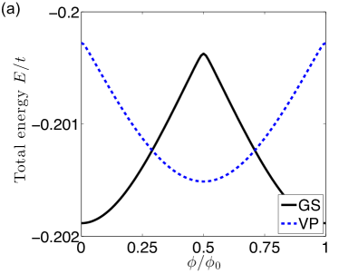
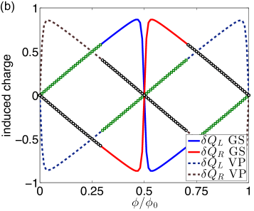
Figure S1: (a) Total energy as function of external flux $\phi/\phi_{0}$ in the charge pumping setup described in the text. Shown are the energy of a solution without visons (GS) and the energy of a solution with a vison pair at the location of the external fluxes (VP). (b) Induced charge at the location of the external fluxes (L) and (R) for the two solutions (GS) and (VP).

Charge pumping in the CI*

To study the charge pumping in the CI* phase, we considered a finite system with $16\times 16$ unit cells and periodic boundary conditions and used $t_{2}=t$ and $U=26t$. A flux $\phi$ was threaded through the center of one hexagon while a flux $-\phi$ was threaded through the center of another hexagon separated by 8 unit cells from the first one.

We compared two different types of (meta-) stable solutions. In the first solution, the $\mathbb{Z}_{2}$ gauge field remains in its ground state configuration, i.e., $\prod_{\hexagon}{\rm sign}(g_{rr^{\prime}})=1$ around each elementary hexagon. We denote this solution as GS in Fig. S1. The second solution places a vison pair at the locations of the external fluxes, i.e., the product $\prod_{\hexagon}{\rm sign}(g_{rr^{\prime}})=-1$ for the two hexagons pierced by the external fluxes. This solution is denoted as VP in Fig. S1.

As demonstrated in Fig. S1(a), the vison pair solution is lowest in energy for a range of external flux $1/4\lesssim\phi/\phi_{0}\lesssim 3/4$. In this parameter regime, it is energetically favorable to (partially) screen the external fluxes by spontaneously creating a vison pair. Note that within the mean-field approximation, there is a level crossing between the two solutions GS and VP. We expect that if the dynamics of the $\mathbb{Z}_{2}$ gauge field is taken into account more accurately, the level crossing will turn into an avoided level crossing. Figure S1(b) shows the induced charge at the positions of the two external fluxes (L) and (R) for the two solutions GS and VP. It becomes clear that the two solutions VP and GS are shifted by $\phi_{0}/2$ with respect to each other.