Mathematical structure of unit systems

Abstract

We investigate the mathematical structure of unit systems and the relations between them. Looking over the entire set of unit systems, we can find a mathematical structure that is called preorder (or quasi-order). For some pair of unit systems, there exists a relation of preorder such that one unit system is transferable to the other unit system. The transfer (or conversion) is possible only when all of the quantities distinguishable in the latter system are always distinguishable in the former system. By utilizing this structure, we can systematically compare the representations in different unit systems. Especially, the equivalence class of unit systems (EUS) plays an important role because the representations of physical quantities and equations are of the same form in unit systems belonging to an EUS. The dimension of quantities is uniquely defined in each EUS. The EUS’s form a partially ordered set. Using these mathematical structures, unit systems and EUS’s are systematically classified and organized as a hierarchical tree.

I Introduction

A unit system is not simply a collection of units but an organized structure that enables diverse physical quantities to be represented in a unified manner. In order to define a unit system, we first select a few units (quantities), which are referred to as base units. Other units are expressed as products or quotients of the base units and are referred to as derived units si ; gupta . It is a matter of choice how many base units are selected. A unit system with $N$ base units is called an $N$-base unit system.

With regard to unit systems, there are several naive questions: How should the base units be chosen; How many base units should be chosen; How can we convert systematically from one unit system to another; What is the meaning of dimensions of quantities (length, time, and so on) birge ; birge2 ; sommerfeld ; duff ; hehl ; guggenheim .

In principle, the number and choice of base units are somewhat arbitrary. This is the reason why there has been proposed so many unit systems and standardization is strongly needed to avoid tangling of them. Many modern articles on unit systems are focused on the unification of unit systems or on the International System of Units (SI) si ; gupta .

In the present paper, from more general point of view, we investigate the mathematical structure of unit systems and clarify the building principles and the relationship between them.

We will show that a binary relation exists between unit systems. For certain pairs of unit systems, one of them can be derived or is transferable from the other. The transferability relation satisfies the mathematical axioms of preorder (or quasi-order) roman ; bourbaki . For a given pair of unit systems, the possibilities are: 1) one of the unit systems is transferable to the other unit system, 2) both unit systems are transferable to each other (equivalent), or 3) neither unit system is transferable to the other unit system (incomparable). It will be shown that the sorting of unit systems according to this preorder is much more significant than the simple sorting by the number of base units.

Especially, the equivalent case is important because with this relation of equivalence we can classify unit systems into equivalence classes. We call such a class as an equivalence class of unit systems (EUS). We will also find that the set of EUS’s is a partially ordered set. We can draw a hierarchical tree of unit systems and EUS’s by using the preorder and partial order structures. The structure of orders and equivalence greatly helps us to sort out many existing and proposed unit systems. There have been few such general and systematic study on unit systems.

We will find that representations of physical quantities and equations have the same form in unit systems belonging to an EUS. Therefore, the EUS is a proper arena for quantity calculus, which is a very important tool in science and engineering. Quantity calculus is closely connected with dimensional analysis buckingham ; bridgman ; bluman ; porter .

Originally the dimensions of units or quantities are introduced in order to cope with the situation where various units were used for length, mass, and time maxwell1 ; porter . For example, the speed of light can be expressed in different units as, $c_{0}=3\times 10^{8}\,{\mu\Omega\mathrm{m/s}}=6.71\times 10^{8}\,{\mu\Omega\mathrm{\text{miles}/\text{hour}}}=\cdots$. We note that the unit for velocity is always expressed as a unit of length divided by a unit of time. We can write, independently of units, the dimension of $c_{0}$ as $\mathsf{L}^{1}\mathsf{M}^{0}\mathsf{T}^{-1}$, with the dimensions for length $\mathsf{L}$, mass $\mathsf{M}$, and time $\mathsf{T}$. In electromagnetism, however, the situation becomes complicated. For example, in the meter-kilogram-second-ampere (MKSA) system, the dimension for electric charge is $\mathsf{L}^{0}\mathsf{M}^{0}\mathsf{T}^{1}\mathsf{I}^{1}$, where $\mathsf{I}$ is the dimension for electric current, while in the centimeter-gram-second (CGS) Gaussian system, it is $\mathsf{L}^{3/2}\mathsf{M}^{1/2}\mathsf{T}^{-1}$.

Thus the notion of dimensions is in a somewhat ambiguous situation. It has been introduced to be independent of units but in fact depends on unit systems. This situation has been noticed in many articlesguggenheim ; bluman ; porter , but no satisfactory explanation has been given. In this paper, we will show that the dimension is uniquely defined in each EUS but it is dependent on EUS’s. The above contradiction can be solved if we understand that the MKSA and CGS Gaussian systems belong to different EUS’s, while the mechanical MKS and CGS unit systems (and other mechanical unit systems) belong to a same EUS.

In this paper, we mainly use electromagnetic unit systems as examples, because a rich variety of unit systems helps us to fully understand the present theory. It will be easy to apply the theory to other fields.

We only deal with scalar quantities. Generalization to geometric quantities such as vectors, tensors, and differential forms can be made post ; schouten . These multi-component quantities can be constructed from dimensioned scalars as in mathematics these are derived from real numbers.

II Basics of unit systems

II.1 Ensembles of quantities

We consider an ensemble $\varOmega$ that contains all of the physical quantities under consideration. At this stage, we make minimum assumptions on the physical quantities in order to clarify the mathematical structures of unit systems. We assume that for an arbitrary quantity $Q\in\varOmega$, the quantity $cQ$, which is scaled by a real number $c\in\mathbb{R}$, is also contained in $\varOmega$. For such a scaled pair, $Q_{1}$ and $Q_{2}=cQ_{1}$, we define the sum as $Q_{1}+Q_{2}=(1+c)Q_{1}$ and call that $Q_{1}$ and $Q_{2}$ are addible in $\varOmega$. Negative quantities and subtraction can be considered with $c<0$. A sum is not defined for unscaled pairs.

We also assume that for any pair of nonzero quantities $Q,P\in\varOmega$, and for any pair of rational numbers $\alpha,\beta\in\mathbb{Q}$, the quantity $Q^{\alpha}P^{\beta}$ is contained in $\varOmega$. In other words, a product, a quotient, or a (fractional) power of quantities are defined.

II.2 Representation of quantities with base units

We now examine the role of the unit system. To define a unit system, $U$, we choose $N$ quantities $u_{i}\in\varOmega$ $(i=1,2,\ldots,N)$ that are to be referenced in the measurement of general quantities. These quantities are customary referred to as base units. The set of base units is represented by a vector, ${\mathchoice{\mbox{\boldmath$u$}}{\mbox{\boldmath$u$}}{\mbox{\scriptsize\boldmath$u$}}{\mbox{\scriptsize\boldmath$u$}}}=(u_{1},u_{2},\ldots,u_{N})$. A physical quantity $Q\in\varOmega$ is represented as

$$Q_{U}=q_{U}{\mathchoice{\mbox{\boldmath$u$}}{\mbox{\boldmath$u$}}{\mbox{\scriptsize\boldmath$u$}}{\mbox{\scriptsize\boldmath$u$}}}^{{\mathchoice{\mbox{\boldmath$d$}}{\mbox{\boldmath$d$}}{\mbox{\scriptsize\boldmath$d$}}{\mbox{\scriptsize\boldmath$d$}}}},$$ (1)

where $q_{U}=\{Q\}_{U}\in\mathbb{R}$ represents the numerical value and ${\mathchoice{\mbox{\boldmath$u$}}{\mbox{\boldmath$u$}}{\mbox{\scriptsize\boldmath$u$}}{\mbox{\scriptsize\boldmath$u$}}}^{{\mathchoice{\mbox{\boldmath$d$}}{\mbox{\boldmath$d$}}{\mbox{\scriptsize\boldmath$d$}}{\mbox{\scriptsize\boldmath$d$}}}}:=\prod_{i=1}^{N}u_{i}^{d_{i}}=u_{1}^{d_{1}}u_{2}^{d_{2}}\cdots u_{N}^{d_{N}}=[Q]_{U}$ represents the unit. We refer to ${\mathchoice{\mbox{\boldmath$d$}}{\mbox{\boldmath$d$}}{\mbox{\scriptsize\boldmath$d$}}{\mbox{\scriptsize\boldmath$d$}}}=(d_{1},\ldots,d_{N})^{\mbox{\scriptsize T}}\in\mathbb{Q}^{N}$ as the dimensional exponents of $Q$ in the unit system $U$. (The unfamiliar notation ${\mathchoice{\mbox{\boldmath$u$}}{\mbox{\boldmath$u$}}{\mbox{\scriptsize\boldmath$u$}}{\mbox{\scriptsize\boldmath$u$}}}^{{\mathchoice{\mbox{\boldmath$d$}}{\mbox{\boldmath$d$}}{\mbox{\scriptsize\boldmath$d$}}{\mbox{\scriptsize\boldmath$d$}}}}$ is borrowed from the notation ${\mathchoice{\mbox{\boldmath$x$}}{\mbox{\boldmath$x$}}{\mbox{\scriptsize\boldmath$x$}}{\mbox{\scriptsize\boldmath$x$}}}\cdot{\mathchoice{\mbox{\boldmath$y$}}{\mbox{\boldmath$y$}}{\mbox{\scriptsize\boldmath$y$}}{\mbox{\scriptsize\boldmath$y$}}}=\sum_{i=1}^{N}x_{i}y_{i}$ for the vectorial inner product.)

For example, the magnetic flux quantum $\varPhi_{0}(=\hbar/2e)$, defined in terms of Planck’s constant $\hbar$ and the elementary charge $e$, can be represented in the MKSA system with ${\mathchoice{\mbox{\boldmath$u$}}{\mbox{\boldmath$u$}}{\mbox{\scriptsize\boldmath$u$}}{\mbox{\scriptsize\boldmath$u$}}}=({\mu\Omega\mathrm{m}},{\mu\Omega\mathrm{kg}},{\mu\Omega\mathrm{s}},{\mu\Omega\mathrm{A}})$ as $\varPhi_{0U}=2.07\times 10^{-15}\,{\mu\Omega\mathrm{m\,kg\,s^{-2}A^{-1}}}$, where $\{\varPhi_{0}\}_{U}=2.07\times 10^{-15}$, $[\varPhi_{0}]_{U}={\mu\Omega\mathrm{m\,kg\,s^{-2}A^{-1}}}$, and ${\mathchoice{\mbox{\boldmath$d$}}{\mbox{\boldmath$d$}}{\mbox{\scriptsize\boldmath$d$}}{\mbox{\scriptsize\boldmath$d$}}}=(1,1,-2,-1)^{\mbox{\scriptsize T}}$.

Note that Eq. (1) is just a representation, which is dependent on the unit system, and $Q_{U}$ does not designate the quantity itself. birge ; bridgman

The representation $Q_{U}=q_{U}{\mathchoice{\mbox{\boldmath$u$}}{\mbox{\boldmath$u$}}{\mbox{\scriptsize\boldmath$u$}}{\mbox{\scriptsize\boldmath$u$}}}^{{\mathchoice{\mbox{\boldmath$d$}}{\mbox{\boldmath$d$}}{\mbox{\scriptsize\boldmath$d$}}{\mbox{\scriptsize\boldmath$d$}}}}=(q_{U},{\mathchoice{\mbox{\boldmath$d$}}{\mbox{\boldmath$d$}}{\mbox{\scriptsize\boldmath$d$}}{\mbox{\scriptsize\boldmath$d$}}})\in\mathbb{R}\times\mathbb{Q}^{N}$, is derived from the corresponding quantity $Q\in\varOmega$. The mapping $\mathcal{U}:(Q\in\varOmega)\mapsto(Q_{U}\in\mathbb{R}\times\mathbb{Q}^{N})$ must satisfy the following properties:

1. Each base unit $u_{i}\in\varOmega$ is mapped as, $\mathcal{U}(u_{i})=1\times u_{i}^{1}$.

2. For any $Q\in\varOmega$ with $\mathcal{U}(Q)=q_{U}{\mathchoice{\mbox{\boldmath$u$}}{\mbox{\boldmath$u$}}{\mbox{\scriptsize\boldmath$u$}}{\mbox{\scriptsize\boldmath$u$}}}^{{\mathchoice{\mbox{\boldmath$d$}}{\mbox{\boldmath$d$}}{\mbox{\scriptsize\boldmath$d$}}{\mbox{\scriptsize\boldmath$d$}}}}$, and any $c\in\mathbb{R}$,

   $$\mathcal{U}(cQ)=c\,\mathcal{U}(Q)=(cq_{U}){\mathchoice{\mbox{\boldmath$u$}}{\mbox{\boldmath$u$}}{\mbox{\scriptsize\boldmath$u$}}{\mbox{\scriptsize\boldmath$u$}}}^{{\mathchoice{\mbox{\boldmath$d$}}{\mbox{\boldmath$d$}}{\mbox{\scriptsize\boldmath$d$}}{\mbox{\scriptsize\boldmath$d$}}}}.$$ (2)

3. For nonzero quantities $Q,P\in\varOmega$ with representations $\mathcal{U}(Q)=q_{U}{\mathchoice{\mbox{\boldmath$u$}}{\mbox{\boldmath$u$}}{\mbox{\scriptsize\boldmath$u$}}{\mbox{\scriptsize\boldmath$u$}}}^{{\mathchoice{\mbox{\boldmath$d$}}{\mbox{\boldmath$d$}}{\mbox{\scriptsize\boldmath$d$}}{\mbox{\scriptsize\boldmath$d$}}}}$ and $\mathcal{U}(P)=p_{U}{\mathchoice{\mbox{\boldmath$u$}}{\mbox{\boldmath$u$}}{\mbox{\scriptsize\boldmath$u$}}{\mbox{\scriptsize\boldmath$u$}}}^{{\mathchoice{\mbox{\boldmath$b$}}{\mbox{\boldmath$b$}}{\mbox{\scriptsize\boldmath$b$}}{\mbox{\scriptsize\boldmath$b$}}}}$, and for $\alpha,\beta\in\mathbb{Q}$, the quantity $Q^{\alpha}P^{\beta}$ is represented as

   $$\mathcal{U}(Q^{\alpha}P^{\beta})=\mathcal{U}(Q)^{\alpha}\mathcal{U}(P)^{\beta}=(q_{U}^{\alpha}p_{U}^{\beta}){\mathchoice{\mbox{\boldmath$u$}}{\mbox{\boldmath$u$}}{\mbox{\scriptsize\boldmath$u$}}{\mbox{\scriptsize\boldmath$u$}}}^{\alpha{\mathchoice{\mbox{\boldmath$d$}}{\mbox{\boldmath$d$}}{\mbox{\scriptsize\boldmath$d$}}{\mbox{\scriptsize\boldmath$d$}}}+\beta{\mathchoice{\mbox{\boldmath$b$}}{\mbox{\boldmath$b$}}{\mbox{\scriptsize\boldmath$b$}}{\mbox{\scriptsize\boldmath$b$}}}}.$$ (3)

   Here, we can consider ${\mathchoice{\mbox{\boldmath$u$}}{\mbox{\boldmath$u$}}{\mbox{\scriptsize\boldmath$u$}}{\mbox{\scriptsize\boldmath$u$}}}^{\alpha{\mathchoice{\mbox{\boldmath$d$}}{\mbox{\boldmath$d$}}{\mbox{\scriptsize\boldmath$d$}}{\mbox{\scriptsize\boldmath$d$}}}+\beta{\mathchoice{\mbox{\boldmath$b$}}{\mbox{\boldmath$b$}}{\mbox{\scriptsize\boldmath$b$}}{\mbox{\scriptsize\boldmath$b$}}}}$ as a unit for measuring $Q^{\alpha}P^{\beta}$. A unit system that conforms to this condition is said to be coherent.

4. If $Q_{1}$ and $Q_{2}$ are addible in $\varOmega$, then $Q_{1}$ and $Q_{2}$ have the same dimension $d$, and we have $\mathcal{U}(Q_{1}+Q_{2})=\mathcal{U}(Q_{1})+\mathcal{U}(Q_{2})=(q_{1U}+q_{2U}){\mathchoice{\mbox{\boldmath$u$}}{\mbox{\boldmath$u$}}{\mbox{\scriptsize\boldmath$u$}}{\mbox{\scriptsize\boldmath$u$}}}^{{\mathchoice{\mbox{\boldmath$d$}}{\mbox{\boldmath$d$}}{\mbox{\scriptsize\boldmath$d$}}{\mbox{\scriptsize\boldmath$d$}}}}$.

5. Even when $Q$ and $P$ are not addible in $\varOmega$, they may have the same dimension $d$. In this case, we can write $\mathcal{U}(Q)+\mathcal{U}(P)=(q_{U}+p_{U}){\mathchoice{\mbox{\boldmath$u$}}{\mbox{\boldmath$u$}}{\mbox{\scriptsize\boldmath$u$}}{\mbox{\scriptsize\boldmath$u$}}}^{{\mathchoice{\mbox{\boldmath$d$}}{\mbox{\boldmath$d$}}{\mbox{\scriptsize\boldmath$d$}}{\mbox{\scriptsize\boldmath$d$}}}}$, i.e., $Q$ and $P$ become addible in the unit system $U$. The addibility is not universal, but unit-system dependent.

The mapping $\mathcal{U}$ is assumed to be surjective, namely, for any $q_{U}\in\mathbb{R}$ and ${\mathchoice{\mbox{\boldmath$d$}}{\mbox{\boldmath$d$}}{\mbox{\scriptsize\boldmath$d$}}{\mbox{\scriptsize\boldmath$d$}}}\in\mathbb{Q}^{N}$, there corresponds a quantity $Q\in\varOmega$ that satisfies $\mathcal{U}(Q)=q_{U}{\mathchoice{\mbox{\boldmath$u$}}{\mbox{\boldmath$u$}}{\mbox{\scriptsize\boldmath$u$}}{\mbox{\scriptsize\boldmath$u$}}}^{{\mathchoice{\mbox{\boldmath$d$}}{\mbox{\boldmath$d$}}{\mbox{\scriptsize\boldmath$d$}}{\mbox{\scriptsize\boldmath$d$}}}}$.

Thus, the unit system $U=({\mathchoice{\mbox{\boldmath$u$}}{\mbox{\boldmath$u$}}{\mbox{\scriptsize\boldmath$u$}}{\mbox{\scriptsize\boldmath$u$}}},\mathcal{U})$ is characterized with the set of base units $u$ and the mapping $\mathcal{U}:\varOmega\rightarrow\mathbb{R}\times\mathbb{Q}^{N}$. We denote the number of base units as $N=\#U$.

III Preorder of unit systems

III.1 Unit-system dependent distinguishability of quantities

If, in a unit system $U$, the presentations of two quantities $Q$ and $P$ coincide, i.e., $\mathcal{U}(Q)=\mathcal{U}(P)$, then we write $Q\stackrel{{\scriptstyle U}}{{=}}P$. More specifically, $Q\stackrel{{\scriptstyle U}}{{=}}P$ indicates that $q_{U}=p_{U}$ and ${\mathchoice{\mbox{\boldmath$d$}}{\mbox{\boldmath$d$}}{\mbox{\scriptsize\boldmath$d$}}{\mbox{\scriptsize\boldmath$d$}}}={\mathchoice{\mbox{\boldmath$b$}}{\mbox{\boldmath$b$}}{\mbox{\scriptsize\boldmath$b$}}{\mbox{\scriptsize\boldmath$b$}}}$, for $\mathcal{U}(Q)=q_{U}{\mathchoice{\mbox{\boldmath$u$}}{\mbox{\boldmath$u$}}{\mbox{\scriptsize\boldmath$u$}}{\mbox{\scriptsize\boldmath$u$}}}^{{\mathchoice{\mbox{\boldmath$d$}}{\mbox{\boldmath$d$}}{\mbox{\scriptsize\boldmath$d$}}{\mbox{\scriptsize\boldmath$d$}}}}$ and $\mathcal{U}(P)=p_{U}{\mathchoice{\mbox{\boldmath$u$}}{\mbox{\boldmath$u$}}{\mbox{\scriptsize\boldmath$u$}}{\mbox{\scriptsize\boldmath$u$}}}^{{\mathchoice{\mbox{\boldmath$b$}}{\mbox{\boldmath$b$}}{\mbox{\scriptsize\boldmath$b$}}{\mbox{\scriptsize\boldmath$b$}}}}$. Clearly, $Q=P$ in $\varOmega$ implies that $Q\stackrel{{\scriptstyle U}}{{=}}P$, although the converse is not necessarily true. Generally, $Q\stackrel{{\scriptstyle U}}{{=}}P$ does not imply $Q\stackrel{{\scriptstyle V}}{{=}}P$ in another unit system $V$. Thus the equality “$\stackrel{{\scriptstyle U}}{{=}}$” is dependent on unit systems.

We should be careful not to write an equation such as $Q_{U}=Q_{V}$, even when $Q_{U}=\mathcal{U}(Q)$ and $Q_{V}=\mathcal{V}(Q)$ are derived from the same quantity $Q\in\varOmega$. Consider two quantities $Q_{1},Q_{2}\in\varOmega$ that satisfy $Q_{1U}\neq Q_{2U}$ and $Q_{1V}=Q_{2V}$. If we write $Q_{1U}=Q_{1V}$ and $Q_{2U}=Q_{2V}$, then we obtain a contradictory result: $Q_{1U}=Q_{2U}$. A similar situation arises for the matrix representation of vectors, i.e., we cannot write $(x_{1},x_{2})=(x_{1}^{\prime},x_{2}^{\prime})$, even when ${\mathchoice{\mbox{\boldmath$x$}}{\mbox{\boldmath$x$}}{\mbox{\scriptsize\boldmath$x$}}{\mbox{\scriptsize\boldmath$x$}}}=x_{1}{\mathchoice{\mbox{\boldmath$e$}}{\mbox{\boldmath$e$}}{\mbox{\scriptsize\boldmath$e$}}{\mbox{\scriptsize\boldmath$e$}}}_{1}+x_{2}{\mathchoice{\mbox{\boldmath$e$}}{\mbox{\boldmath$e$}}{\mbox{\scriptsize\boldmath$e$}}{\mbox{\scriptsize\boldmath$e$}}}_{2}=x_{1}^{\prime}{\mathchoice{\mbox{\boldmath$e$}}{\mbox{\boldmath$e$}}{\mbox{\scriptsize\boldmath$e$}}{\mbox{\scriptsize\boldmath$e$}}}_{1}^{\prime}+x_{2}^{\prime}{\mathchoice{\mbox{\boldmath$e$}}{\mbox{\boldmath$e$}}{\mbox{\scriptsize\boldmath$e$}}{\mbox{\scriptsize\boldmath$e$}}}_{2}^{\prime}$.

The relation “$\stackrel{{\scriptstyle U}}{{=}}$” is an equivalence relation roman . Symmetry, reflexivity, and transitivity hold, i.e., (1) $Q\stackrel{{\scriptstyle U}}{{=}}Q^{\prime}$ implies $Q^{\prime}\stackrel{{\scriptstyle U}}{{=}}Q$, (2) $Q\stackrel{{\scriptstyle U}}{{=}}Q$, and (3) $Q\stackrel{{\scriptstyle U}}{{=}}Q^{\prime}$ and $Q^{\prime}\stackrel{{\scriptstyle U}}{{=}}Q^{\prime\prime}$ imply $Q^{\prime}\stackrel{{\scriptstyle U}}{{=}}Q^{\prime\prime}$, for all $Q$, $Q^{\prime}$, and $Q^{\prime\prime}\in\varOmega$.

III.2 Transferability of unit systems

For a certain pair of unit systems, $U$ and $V$, if $(Q\stackrel{{\scriptstyle U}}{{=}}P)\Rightarrow(Q\stackrel{{\scriptstyle V}}{{=}}P)$ holds for any pairs of quantities, $Q$, $P\in\varOmega$, we then denote

$$U\succsim V.$$ (4)

This relation means that the quantities that are considered to be equal in $U$ are always considered to be equal in $V$. In other words, two quantities that are distinguishable in $V$ are always distinguishable in $U$. Then, we say that the unit system $U$ is transferable to the unit system $V$, or $V$ is transferable from $U$.

The relation “$\succsim$” satisfies the axioms of preorder (or quasi-order); reflexivity and transitivity. Namely, (1) $U\succsim U$, and (2) $U\succsim U^{\prime}$ and $U^{\prime}\succsim U^{\prime\prime}$ imply $U\succsim U^{\prime\prime}$, for all $U$, $U^{\prime}$, and $U^{\prime\prime}$. Thus, the set of unit systems is a preordered set (poset) roman ; bourbaki . This is the key to understanding the global structure of unit systems.

When both $U\succsim V$ and $U\precsim V$ are satisfied, i.e., $U$ and $V$ are bilaterally transferable, we write $U\sim V$, and $U$ and $V$ are called to be equivalent.

There may be cases in which neither $U\succsim V$ nor $U\precsim V$ are satisfied, namely, $U$ and $V$ are transferable in neither direction. In this case, we write $U\parallel V$, and say that $U$ and $V$ are incomparable. Moreover, if $U\succsim V$ and $V\not\succsim U$, then, $U$ is strictly transferable to $V$ and we write $U\succ V$. The relations are listed in Table 1.

	$U\precsim V$	$U\not\precsim V$
$U\succsim V$	$U\sim V$ ($N=M$)	$U\succ V$ ($N>M$)
$U\not\succsim V$	$U\prec V$ ($N<M$)	$U\parallel V$ ($N<=>M$)

Table 1: Four possible relations between two unit systems $U$ and $V$: (strictly) transferable to ($\succ$), (strictly) transferable from ($\prec$), equivalent ($\sim$), and incomparable ($\parallel$). The relations between $N=\#U$ and $M=\#V$, which are the numbers of base units, are also listed.

IV Conversion of unit systems

IV.1 Mapping from one unit system to another

We consider two unit systems, $U=({\mathchoice{\mbox{\boldmath$u$}}{\mbox{\boldmath$u$}}{\mbox{\scriptsize\boldmath$u$}}{\mbox{\scriptsize\boldmath$u$}}},\mathcal{U})$ and $V=({\mathchoice{\mbox{\boldmath$v$}}{\mbox{\boldmath$v$}}{\mbox{\scriptsize\boldmath$v$}}{\mbox{\scriptsize\boldmath$v$}}},\mathcal{V})$ and assume that $U\succsim V$. We will show that only in such cases there exists a mapping $\mathcal{T}$ from $\mathcal{U}(\varOmega)=\mathbb{R}\times\mathbb{Q}^{N}$ to $\mathcal{V}(\varOmega)=\mathbb{R}\times\mathbb{Q}^{M}$.

First, as shown in Fig. 1, we choose an arbitrary representation $Q_{U}\in\mathbb{R}\times\mathbb{Q}^{N}$ in $U$. There is a non-empty preimage (inverse image) $\mathcal{U}^{-1}(Q_{U})\subset\varOmega$ because $\mathcal{U}$ is surjective. $\mathcal{U}^{-1}(Q_{U})$ does not mean an inverse mapping but just designates a set containing all quantities that is mapped to $Q_{U}$ with $\mathcal{U}$. The quantities in $\mathcal{U}^{-1}(Q_{U})$ cannot be distinguished in $U$. By choosing a quantity $Q$ in $\mathcal{U}^{-1}(Q_{U})$ and mapping it with $\mathcal{V}$, we obtain $Q_{V}$. Its preimage $\mathcal{V}^{-1}(Q_{V})$ consists of the quantities that cannot be distinguished in $V$. From the assumption that $U\succsim V$, $\mathcal{V}^{-1}(Q_{V})$ should include $\mathcal{U}^{-1}(Q_{U})$, i.e., $\mathcal{V}^{-1}(Q_{V})\supseteq\mathcal{U}^{-1}(Q_{U})$. Therefore, for a given $Q_{U}$, $Q_{V}$ is uniquely determined with $\mathcal{V}(\mathcal{U}^{-1}(Q_{U}))=Q_{V}$. Thus, we obtain a mapping (surjection) $\mathcal{T}:Q_{U}\in\mathcal{U}(\varOmega)\mapsto Q_{V}\in\mathcal{V}(\varOmega)$, or $\mathcal{T}:U\rightarrow V$.

The following relations hold for $\mathcal{T}$: for $c\in\mathbb{R}$, and $Q_{U}$ in $U$, $\mathcal{T}(cQ_{U})=c\mathcal{T}(Q_{U})$; for $\alpha,\beta\in\mathbb{Q}$, and $Q_{U}$, $P_{U}$ in $U$, $\mathcal{T}(Q_{U}^{\alpha}P_{U}^{\beta})=\mathcal{T}(Q_{U})^{\alpha}\mathcal{T}(P_{U})^{\beta}$; for $Q_{1U}$, $Q_{2U}$, which are addible in $U$, $\mathcal{T}(Q_{1U}+Q_{2U})=\mathcal{T}(Q_{1U})+\mathcal{T}(Q_{2U})$.

Note that if $U\succsim V$, then $N\geq M$, where $N=\#U$ and $M=\#V$. Therefore, for $U\sim V$, we have $N=M$, and the mapping $\mathcal{T}$ is reversible. For $U\parallel V$, no mapping exits, and no definite relation between $N$ and $M$ exists. (See Table 1.)

Figure 1: Ordering of unit systems $U$ and $V$. A quantity $Q\in\varOmega$ is mapped to $\mathcal{U}(Q)$ and $\mathcal{V}(Q)$ for the representation in the respective unit systems. In the case of $U\succsim V$, the preimage $\mathcal{U}^{-1}(Q_{U})$ is always included in $\mathcal{V}^{-1}(Q_{V})$. Only then we can naturally define the mapping $\mathcal{T}:Q_{U}\mapsto Q_{V}=\mathcal{V}(\mathcal{U}^{-1}(Q_{U}))$.

IV.2 Transfer matrix

Let us consider two unit systems $U=({\mathchoice{\mbox{\boldmath$u$}}{\mbox{\boldmath$u$}}{\mbox{\scriptsize\boldmath$u$}}{\mbox{\scriptsize\boldmath$u$}}},\mathcal{U})$, ${\mathchoice{\mbox{\boldmath$u$}}{\mbox{\boldmath$u$}}{\mbox{\scriptsize\boldmath$u$}}{\mbox{\scriptsize\boldmath$u$}}}=(u_{1},u_{2},\cdots,u_{N})$ and $V=({\mathchoice{\mbox{\boldmath$v$}}{\mbox{\boldmath$v$}}{\mbox{\scriptsize\boldmath$v$}}{\mbox{\scriptsize\boldmath$v$}}},\mathcal{V})$, ${\mathchoice{\mbox{\boldmath$v$}}{\mbox{\boldmath$v$}}{\mbox{\scriptsize\boldmath$v$}}{\mbox{\scriptsize\boldmath$v$}}}=(v_{1},v_{2},\cdots,u_{M})$, satisfying $U\succsim V$ and $N\geq M$. A quantity $Q\in\varOmega$ is represented in $U$ and $V$, respectively, as follows:

$$\mathcal{U}(Q)=Q_{U}=q_{U}{\mathchoice{\mbox{\boldmath$u$}}{\mbox{\boldmath$u$}}{\mbox{\scriptsize\boldmath$u$}}{\mbox{\scriptsize\boldmath$u$}}}^{{\mathchoice{\mbox{\boldmath$d$}}{\mbox{\boldmath$d$}}{\mbox{\scriptsize\boldmath$d$}}{\mbox{\scriptsize\boldmath$d$}}}},\quad\mathcal{V}(Q)=Q_{V}=q_{V}{\mathchoice{\mbox{\boldmath$v$}}{\mbox{\boldmath$v$}}{\mbox{\scriptsize\boldmath$v$}}{\mbox{\scriptsize\boldmath$v$}}}^{{\mathchoice{\mbox{\boldmath$c$}}{\mbox{\boldmath$c$}}{\mbox{\scriptsize\boldmath$c$}}{\mbox{\scriptsize\boldmath$c$}}}},$$ (5)

where $q_{U},q_{V}\in\mathbb{R}$, ${\mathchoice{\mbox{\boldmath$d$}}{\mbox{\boldmath$d$}}{\mbox{\scriptsize\boldmath$d$}}{\mbox{\scriptsize\boldmath$d$}}}=(d_{1},d_{2},\ldots,d_{N})^{\mbox{\scriptsize T}}\in\mathbb{Q}^{N}$, and ${\mathchoice{\mbox{\boldmath$c$}}{\mbox{\boldmath$c$}}{\mbox{\scriptsize\boldmath$c$}}{\mbox{\scriptsize\boldmath$c$}}}=(c_{1},c_{2},\ldots,c_{M})^{\mbox{\scriptsize T}}\in\mathbb{Q}^{M}$. As described in Sec. IV A, the relation between these representations can be implemented as a mapping $Q_{V}=\mathcal{T}(Q_{U})$.

The explicit form of $\mathcal{T}$ can be obtained as follows. Each base unit $u_{i}\in\varOmega$ $(i=1,\ldots,N)$ of $U$ can be considered to be a representation in $U$ with $\mathcal{U}(u_{i})=u_{iU}=1\times u_{i}^{1}$, and can therefore be mapped by $\mathcal{T}$. On the other hand, we have the representation of $u_{i}\in\varOmega$ in $V$ as $\mathcal{V}(u_{i})=k_{i}{\mathchoice{\mbox{\boldmath$v$}}{\mbox{\boldmath$v$}}{\mbox{\scriptsize\boldmath$v$}}{\mbox{\scriptsize\boldmath$v$}}}^{{\mathchoice{\mbox{\boldmath$t$}}{\mbox{\boldmath$t$}}{\mbox{\scriptsize\boldmath$t$}}{\mbox{\scriptsize\boldmath$t$}}}_{i}}$, where $k_{i}\in\mathbb{R}_{+}$ (positive real), ${\mathchoice{\mbox{\boldmath$t$}}{\mbox{\boldmath$t$}}{\mbox{\scriptsize\boldmath$t$}}{\mbox{\scriptsize\boldmath$t$}}}_{i}=(t_{1i},\ldots,t_{Mi})^{\mbox{\scriptsize T}}$, $t_{ji}\in\mathbb{Q}$ $(j=1,\ldots,M)$. From these expressions, we have $\mathcal{T}(u_{iU})=k_{i}{\mathchoice{\mbox{\boldmath$v$}}{\mbox{\boldmath$v$}}{\mbox{\scriptsize\boldmath$v$}}{\mbox{\scriptsize\boldmath$v$}}}^{{\mathchoice{\mbox{\boldmath$t$}}{\mbox{\boldmath$t$}}{\mbox{\scriptsize\boldmath$t$}}{\mbox{\scriptsize\boldmath$t$}}}_{i}}$.

Now we can map the representation $\mathcal{U}(Q)=Q_{U}=q_{U}{\mathchoice{\mbox{\boldmath$u$}}{\mbox{\boldmath$u$}}{\mbox{\scriptsize\boldmath$u$}}{\mbox{\scriptsize\boldmath$u$}}}^{{\mathchoice{\mbox{\boldmath$d$}}{\mbox{\boldmath$d$}}{\mbox{\scriptsize\boldmath$d$}}{\mbox{\scriptsize\boldmath$d$}}}}$ of an arbitrary quantity $Q\in\varOmega$ as

$$Q_{V}=\mathcal{T}(Q_{U})=\mathcal{T}(q_{U}{\mathchoice{\mbox{\boldmath$u$}}{\mbox{\boldmath$u$}}{\mbox{\scriptsize\boldmath$u$}}{\mbox{\scriptsize\boldmath$u$}}}^{{\mathchoice{\mbox{\boldmath$d$}}{\mbox{\boldmath$d$}}{\mbox{\scriptsize\boldmath$d$}}{\mbox{\scriptsize\boldmath$d$}}}})=q_{U}\prod_{i=1}^{N}k_{i}^{d_{i}}{\mathchoice{\mbox{\boldmath$v$}}{\mbox{\boldmath$v$}}{\mbox{\scriptsize\boldmath$v$}}{\mbox{\scriptsize\boldmath$v$}}}^{\sum_{i=1}^{N}{\mathchoice{\mbox{\boldmath$t$}}{\mbox{\boldmath$t$}}{\mbox{\scriptsize\boldmath$t$}}{\mbox{\scriptsize\boldmath$t$}}}_{i}d_{i}}=q_{V}{\mathchoice{\mbox{\boldmath$v$}}{\mbox{\boldmath$v$}}{\mbox{\scriptsize\boldmath$v$}}{\mbox{\scriptsize\boldmath$v$}}}^{{\mathchoice{\mbox{\boldmath$c$}}{\mbox{\boldmath$c$}}{\mbox{\scriptsize\boldmath$c$}}{\mbox{\scriptsize\boldmath$c$}}}},\quad\text{with}\quad q_{V}=q_{U}{\mathchoice{\mbox{\boldmath$k$}}{\mbox{\boldmath$k$}}{\mbox{\scriptsize\boldmath$k$}}{\mbox{\scriptsize\boldmath$k$}}}^{{\mathchoice{\mbox{\boldmath$d$}}{\mbox{\boldmath$d$}}{\mbox{\scriptsize\boldmath$d$}}{\mbox{\scriptsize\boldmath$d$}}}},\quad{\mathchoice{\mbox{\boldmath$c$}}{\mbox{\boldmath$c$}}{\mbox{\scriptsize\boldmath$c$}}{\mbox{\scriptsize\boldmath$c$}}}=T{\mathchoice{\mbox{\boldmath$d$}}{\mbox{\boldmath$d$}}{\mbox{\scriptsize\boldmath$d$}}{\mbox{\scriptsize\boldmath$d$}}},$$ (6)

where $T=[{\mathchoice{\mbox{\boldmath$t$}}{\mbox{\boldmath$t$}}{\mbox{\scriptsize\boldmath$t$}}{\mbox{\scriptsize\boldmath$t$}}}_{1},{\mathchoice{\mbox{\boldmath$t$}}{\mbox{\boldmath$t$}}{\mbox{\scriptsize\boldmath$t$}}{\mbox{\scriptsize\boldmath$t$}}}_{2},\cdots,{\mathchoice{\mbox{\boldmath$t$}}{\mbox{\boldmath$t$}}{\mbox{\scriptsize\boldmath$t$}}{\mbox{\scriptsize\boldmath$t$}}}_{N}]$ is an $M\times N$ matrix and ${\mathchoice{\mbox{\boldmath$k$}}{\mbox{\boldmath$k$}}{\mbox{\scriptsize\boldmath$k$}}{\mbox{\scriptsize\boldmath$k$}}}^{{\mathchoice{\mbox{\boldmath$d$}}{\mbox{\boldmath$d$}}{\mbox{\scriptsize\boldmath$d$}}{\mbox{\scriptsize\boldmath$d$}}}}:=\prod_{i=1}^{N}k_{i}^{d_{i}}=k_{1}^{d_{1}}\cdots k_{N}^{d_{N}}$. We refer to $T$ as a transfer matrix and assume that $\mathrm{rank}\,T=M$.

Thus, the mapping $\mathcal{T}:Q_{U}\mapsto Q_{V}$ is characterized by a vector ${\mathchoice{\mbox{\boldmath$k$}}{\mbox{\boldmath$k$}}{\mbox{\scriptsize\boldmath$k$}}{\mbox{\scriptsize\boldmath$k$}}}=(k_{1},k_{2},\ldots,k_{N})^{\mbox{\scriptsize T}}\in\mathbb{R}_{+}^{N}$ and a linear map $T\in L(\mathbb{Q}^{N}\rightarrow\mathbb{Q}^{M})$. Thus, we can write $\mathcal{T}=({\mathchoice{\mbox{\boldmath$k$}}{\mbox{\boldmath$k$}}{\mbox{\scriptsize\boldmath$k$}}{\mbox{\scriptsize\boldmath$k$}}},T)$.

Equation (6) indicates that, for ${\mathchoice{\mbox{\boldmath$d$}}{\mbox{\boldmath$d$}}{\mbox{\scriptsize\boldmath$d$}}{\mbox{\scriptsize\boldmath$d$}}}=0$, $Q_{V}=Q_{U}\,(=q_{U})$ holds, i.e., the dimensionless representations are conserved under the mapping.

IV.3 Composition of transformations

The composition of transformations can easily be constructed. Consider the mappings: $\mathcal{T}=({\mathchoice{\mbox{\boldmath$k$}}{\mbox{\boldmath$k$}}{\mbox{\scriptsize\boldmath$k$}}{\mbox{\scriptsize\boldmath$k$}}},T)$ and $\mathcal{S}=({\mathchoice{\mbox{\boldmath$h$}}{\mbox{\boldmath$h$}}{\mbox{\scriptsize\boldmath$h$}}{\mbox{\scriptsize\boldmath$h$}}},S)$, with $U\stackrel{{\scriptstyle\mathcal{T}}}{{\rightarrow}}V\stackrel{{\scriptstyle\mathcal{S}}}{{\rightarrow}}W$. From $Q_{V}=\mathcal{T}(Q_{U})=q_{U}{\mathchoice{\mbox{\boldmath$k$}}{\mbox{\boldmath$k$}}{\mbox{\scriptsize\boldmath$k$}}{\mbox{\scriptsize\boldmath$k$}}}^{{\mathchoice{\mbox{\boldmath$d$}}{\mbox{\boldmath$d$}}{\mbox{\scriptsize\boldmath$d$}}{\mbox{\scriptsize\boldmath$d$}}}}{\mathchoice{\mbox{\boldmath$v$}}{\mbox{\boldmath$v$}}{\mbox{\scriptsize\boldmath$v$}}{\mbox{\scriptsize\boldmath$v$}}}^{T{\mathchoice{\mbox{\boldmath$d$}}{\mbox{\boldmath$d$}}{\mbox{\scriptsize\boldmath$d$}}{\mbox{\scriptsize\boldmath$d$}}}}$ and $\mathcal{S}(Q_{V})=q_{V}{\mathchoice{\mbox{\boldmath$h$}}{\mbox{\boldmath$h$}}{\mbox{\scriptsize\boldmath$h$}}{\mbox{\scriptsize\boldmath$h$}}}^{{\mathchoice{\mbox{\boldmath$c$}}{\mbox{\boldmath$c$}}{\mbox{\scriptsize\boldmath$c$}}{\mbox{\scriptsize\boldmath$c$}}}}{\mathchoice{\mbox{\boldmath$w$}}{\mbox{\boldmath$w$}}{\mbox{\scriptsize\boldmath$w$}}{\mbox{\scriptsize\boldmath$w$}}}^{S{\mathchoice{\mbox{\boldmath$c$}}{\mbox{\boldmath$c$}}{\mbox{\scriptsize\boldmath$c$}}{\mbox{\scriptsize\boldmath$c$}}}}$, we have the composite mapping:

$$\mathcal{S}\mathcal{T}(Q_{U})=q_{U}{\mathchoice{\mbox{\boldmath$k$}}{\mbox{\boldmath$k$}}{\mbox{\scriptsize\boldmath$k$}}{\mbox{\scriptsize\boldmath$k$}}}^{{\mathchoice{\mbox{\boldmath$d$}}{\mbox{\boldmath$d$}}{\mbox{\scriptsize\boldmath$d$}}{\mbox{\scriptsize\boldmath$d$}}}}{\mathchoice{\mbox{\boldmath$h$}}{\mbox{\boldmath$h$}}{\mbox{\scriptsize\boldmath$h$}}{\mbox{\scriptsize\boldmath$h$}}}^{(T{\mathchoice{\mbox{\boldmath$d$}}{\mbox{\boldmath$d$}}{\mbox{\scriptsize\boldmath$d$}}{\mbox{\scriptsize\boldmath$d$}}})}{\mathchoice{\mbox{\boldmath$w$}}{\mbox{\boldmath$w$}}{\mbox{\scriptsize\boldmath$w$}}{\mbox{\scriptsize\boldmath$w$}}}^{S(T{\mathchoice{\mbox{\boldmath$d$}}{\mbox{\boldmath$d$}}{\mbox{\scriptsize\boldmath$d$}}{\mbox{\scriptsize\boldmath$d$}}})}=q_{U}({\mathchoice{\mbox{\boldmath$k$}}{\mbox{\boldmath$k$}}{\mbox{\scriptsize\boldmath$k$}}{\mbox{\scriptsize\boldmath$k$}}}{\mathchoice{\mbox{\boldmath$h$}}{\mbox{\boldmath$h$}}{\mbox{\scriptsize\boldmath$h$}}{\mbox{\scriptsize\boldmath$h$}}}^{T})^{{\mathchoice{\mbox{\boldmath$d$}}{\mbox{\boldmath$d$}}{\mbox{\scriptsize\boldmath$d$}}{\mbox{\scriptsize\boldmath$d$}}}}{\mathchoice{\mbox{\boldmath$w$}}{\mbox{\boldmath$w$}}{\mbox{\scriptsize\boldmath$w$}}{\mbox{\scriptsize\boldmath$w$}}}^{(ST){\mathchoice{\mbox{\boldmath$d$}}{\mbox{\boldmath$d$}}{\mbox{\scriptsize\boldmath$d$}}{\mbox{\scriptsize\boldmath$d$}}}}.$$ (7)

Here, we have used

$${\mathchoice{\mbox{\boldmath$h$}}{\mbox{\boldmath$h$}}{\mbox{\scriptsize\boldmath$h$}}{\mbox{\scriptsize\boldmath$h$}}}^{(T{\mathchoice{\mbox{\boldmath$d$}}{\mbox{\boldmath$d$}}{\mbox{\scriptsize\boldmath$d$}}{\mbox{\scriptsize\boldmath$d$}}})}=\prod_{j=1}^{M}h_{j}^{\sum_{i=1}^{N}T_{ji}d_{i}}=\prod_{i=1}^{N}\prod_{j=1}^{M}h_{j}^{T_{ji}d_{i}}=({\mathchoice{\mbox{\boldmath$h$}}{\mbox{\boldmath$h$}}{\mbox{\scriptsize\boldmath$h$}}{\mbox{\scriptsize\boldmath$h$}}}^{T})^{{\mathchoice{\mbox{\boldmath$d$}}{\mbox{\boldmath$d$}}{\mbox{\scriptsize\boldmath$d$}}{\mbox{\scriptsize\boldmath$d$}}}},$$ (8)

with $({\mathchoice{\mbox{\boldmath$h$}}{\mbox{\boldmath$h$}}{\mbox{\scriptsize\boldmath$h$}}{\mbox{\scriptsize\boldmath$h$}}}^{T})_{i}=\prod_{j=1}^{M}h_{j}^{T_{ji}}$ $(i=1,\ldots,N)$, and ${\mathchoice{\mbox{\boldmath$k$}}{\mbox{\boldmath$k$}}{\mbox{\scriptsize\boldmath$k$}}{\mbox{\scriptsize\boldmath$k$}}}^{{\mathchoice{\mbox{\boldmath$d$}}{\mbox{\boldmath$d$}}{\mbox{\scriptsize\boldmath$d$}}{\mbox{\scriptsize\boldmath$d$}}}}{\mathchoice{\mbox{\boldmath$k$}}{\mbox{\boldmath$k$}}{\mbox{\scriptsize\boldmath$k$}}{\mbox{\scriptsize\boldmath$k$}}}^{\prime{\mathchoice{\mbox{\boldmath$d$}}{\mbox{\boldmath$d$}}{\mbox{\scriptsize\boldmath$d$}}{\mbox{\scriptsize\boldmath$d$}}}}=({\mathchoice{\mbox{\boldmath$k$}}{\mbox{\boldmath$k$}}{\mbox{\scriptsize\boldmath$k$}}{\mbox{\scriptsize\boldmath$k$}}}{\mathchoice{\mbox{\boldmath$k$}}{\mbox{\boldmath$k$}}{\mbox{\scriptsize\boldmath$k$}}{\mbox{\scriptsize\boldmath$k$}}}^{\prime})^{{\mathchoice{\mbox{\boldmath$d$}}{\mbox{\boldmath$d$}}{\mbox{\scriptsize\boldmath$d$}}{\mbox{\scriptsize\boldmath$d$}}}}$ with ${\mathchoice{\mbox{\boldmath$k$}}{\mbox{\boldmath$k$}}{\mbox{\scriptsize\boldmath$k$}}{\mbox{\scriptsize\boldmath$k$}}}{\mathchoice{\mbox{\boldmath$k$}}{\mbox{\boldmath$k$}}{\mbox{\scriptsize\boldmath$k$}}{\mbox{\scriptsize\boldmath$k$}}}^{\prime}=(k_{1}k^{\prime}_{1},\ldots,k_{N}k^{\prime}_{N})$. From Eq. (7), we have the composition rule:

$$\mathcal{S}\mathcal{T}=({\mathchoice{\mbox{\boldmath$h$}}{\mbox{\boldmath$h$}}{\mbox{\scriptsize\boldmath$h$}}{\mbox{\scriptsize\boldmath$h$}}}^{T}{\mathchoice{\mbox{\boldmath$k$}}{\mbox{\boldmath$k$}}{\mbox{\scriptsize\boldmath$k$}}{\mbox{\scriptsize\boldmath$k$}}},ST).$$ (9)

We consider two invertible mappings $\mathcal{T}=({\mathchoice{\mbox{\boldmath$k$}}{\mbox{\boldmath$k$}}{\mbox{\scriptsize\boldmath$k$}}{\mbox{\scriptsize\boldmath$k$}}},T):U\rightarrow U^{\prime}$, $\mathcal{S}=({\mathchoice{\mbox{\boldmath$h$}}{\mbox{\boldmath$h$}}{\mbox{\scriptsize\boldmath$h$}}{\mbox{\scriptsize\boldmath$h$}}},S):U^{\prime}\rightarrow U$. The composite mapping $\mathcal{S}\mathcal{T}=({\mathchoice{\mbox{\boldmath$h$}}{\mbox{\boldmath$h$}}{\mbox{\scriptsize\boldmath$h$}}{\mbox{\scriptsize\boldmath$h$}}}^{T}{\mathchoice{\mbox{\boldmath$k$}}{\mbox{\boldmath$k$}}{\mbox{\scriptsize\boldmath$k$}}{\mbox{\scriptsize\boldmath$k$}}},ST)$ becomes the identity mapping $\mathcal{I}=({\mathchoice{\mbox{\boldmath$1$}}{\mbox{\boldmath$1$}}{\mbox{\scriptsize\boldmath$1$}}{\mbox{\scriptsize\boldmath$1$}}}_{N},I)$, if ${\mathchoice{\mbox{\boldmath$h$}}{\mbox{\boldmath$h$}}{\mbox{\scriptsize\boldmath$h$}}{\mbox{\scriptsize\boldmath$h$}}}={\mathchoice{\mbox{\boldmath$k$}}{\mbox{\boldmath$k$}}{\mbox{\scriptsize\boldmath$k$}}{\mbox{\scriptsize\boldmath$k$}}}^{-T^{-1}}$ and $S=T^{-1}$ are satisfied. Here, we have introduced an $N$ dimensional vector ${\mathchoice{\mbox{\boldmath$1$}}{\mbox{\boldmath$1$}}{\mbox{\scriptsize\boldmath$1$}}{\mbox{\scriptsize\boldmath$1$}}}_{N}=(1,1,\ldots,1)^{\mbox{\scriptsize T}}$. In other words, the inversion of mapping $\mathcal{T}=({\mathchoice{\mbox{\boldmath$k$}}{\mbox{\boldmath$k$}}{\mbox{\scriptsize\boldmath$k$}}{\mbox{\scriptsize\boldmath$k$}}},T)$ is given as

$$\mathcal{T}^{-1}=({\mathchoice{\mbox{\boldmath$k$}}{\mbox{\boldmath$k$}}{\mbox{\scriptsize\boldmath$k$}}{\mbox{\scriptsize\boldmath$k$}}}^{-T^{-1}},T^{-1}).$$ (10)

V Quantities in equivalent unit systems

V.1 Equivalence class of unit systems

In the case of $U\sim V$, the transformation $\mathcal{T}$ is invertible and therefore the square ($N=M$) matrix $T$ is regular. In this case, the two unit systems are basically the same because there is a one-to-one correspondence between their representations, and we can safely write $Q_{U}=Q_{V}$.

The relation “$\sim$” is an equivalence relation. Therefore, according to this relation, we can classify $N$-base unit systems. We refer to each class as an equivalence class of unit systems (EUS). Unit systems that belong to different EUS’s are incomparable.

If we do not transcend the border of an EUS, then the representations $Q_{U}$ and $Q_{V}$ and the corresponding preimages $\mathcal{U}^{-1}(Q_{U})=\mathcal{V}^{-1}(Q_{V})$ in $\varOmega$ can be identified. As almost unconsciously we are doing, we can write all of these representations as $Q$, because there is no way to distinguish the members in the preimages within these unit systems.

For example, the MKS$\Omega$ (due to G. Giorgi) and MKSA systems are equivalent, and we can write $1.2\,{\mu\Omega\mathrm{O}}=1.2\,{\mu\Omega\mathrm{m^{2}kg\,s^{-3}A^{-2}}}\,(=R)$. The CGS and MKS unit systems, both purely mechanical, are equivalent, and we can write $1\,{\mu\Omega\mathrm{erg}}=10^{-7}\,{\mu\Omega\mathrm{J}}\,(=E)$.

V.2 Relation among equivalence classes of unit systems — partial order

Let us consider a set of unit systems that is equivalent to a unit system $U$. We write such an equivalence class of unit systems (EUS) as $\mathscr{U}=\{U,U^{\prime},\ldots\}$. For any pair of the unit systems, there is an invertible mapping like $\mathcal{D}=({\mathchoice{\mbox{\boldmath$k$}}{\mbox{\boldmath$k$}}{\mbox{\scriptsize\boldmath$k$}}{\mbox{\scriptsize\boldmath$k$}}},D):U\rightarrow U^{\prime}$. Then we have

$$q_{U}{\mathchoice{\mbox{\boldmath$u$}}{\mbox{\boldmath$u$}}{\mbox{\scriptsize\boldmath$u$}}{\mbox{\scriptsize\boldmath$u$}}}^{{\mathchoice{\mbox{\boldmath$d$}}{\mbox{\boldmath$d$}}{\mbox{\scriptsize\boldmath$d$}}{\mbox{\scriptsize\boldmath$d$}}}}=q_{U}{\mathchoice{\mbox{\boldmath$k$}}{\mbox{\boldmath$k$}}{\mbox{\scriptsize\boldmath$k$}}{\mbox{\scriptsize\boldmath$k$}}}^{{\mathchoice{\mbox{\boldmath$d$}}{\mbox{\boldmath$d$}}{\mbox{\scriptsize\boldmath$d$}}{\mbox{\scriptsize\boldmath$d$}}}}{\mathchoice{\mbox{\boldmath$k$}}{\mbox{\boldmath$k$}}{\mbox{\scriptsize\boldmath$k$}}{\mbox{\scriptsize\boldmath$k$}}}^{-{\mathchoice{\mbox{\boldmath$d$}}{\mbox{\boldmath$d$}}{\mbox{\scriptsize\boldmath$d$}}{\mbox{\scriptsize\boldmath$d$}}}}{\mathchoice{\mbox{\boldmath$u$}}{\mbox{\boldmath$u$}}{\mbox{\scriptsize\boldmath$u$}}{\mbox{\scriptsize\boldmath$u$}}}^{{\mathchoice{\mbox{\boldmath$d$}}{\mbox{\boldmath$d$}}{\mbox{\scriptsize\boldmath$d$}}{\mbox{\scriptsize\boldmath$d$}}}}=q_{U^{\prime}}({\mathchoice{\mbox{\boldmath$k$}}{\mbox{\boldmath$k$}}{\mbox{\scriptsize\boldmath$k$}}{\mbox{\scriptsize\boldmath$k$}}}^{-1}{\mathchoice{\mbox{\boldmath$u$}}{\mbox{\boldmath$u$}}{\mbox{\scriptsize\boldmath$u$}}{\mbox{\scriptsize\boldmath$u$}}})^{{\mathchoice{\mbox{\boldmath$d$}}{\mbox{\boldmath$d$}}{\mbox{\scriptsize\boldmath$d$}}{\mbox{\scriptsize\boldmath$d$}}}}=q_{U^{\prime}}({\mathchoice{\mbox{\boldmath$k$}}{\mbox{\boldmath$k$}}{\mbox{\scriptsize\boldmath$k$}}{\mbox{\scriptsize\boldmath$k$}}}^{-1}{\mathchoice{\mbox{\boldmath$u$}}{\mbox{\boldmath$u$}}{\mbox{\scriptsize\boldmath$u$}}{\mbox{\scriptsize\boldmath$u$}}})^{D^{-1}D{\mathchoice{\mbox{\boldmath$d$}}{\mbox{\boldmath$d$}}{\mbox{\scriptsize\boldmath$d$}}{\mbox{\scriptsize\boldmath$d$}}}}=q_{U^{\prime}}{\mathchoice{\mbox{\boldmath$u$}}{\mbox{\boldmath$u$}}{\mbox{\scriptsize\boldmath$u$}}{\mbox{\scriptsize\boldmath$u$}}}^{\prime{\mathchoice{\mbox{\boldmath$d$}}{\mbox{\boldmath$d$}}{\mbox{\scriptsize\boldmath$d$}}{\mbox{\scriptsize\boldmath$d$}}}^{\prime}},$$ (11)

where $q_{U^{\prime}}=q_{U}{\mathchoice{\mbox{\boldmath$k$}}{\mbox{\boldmath$k$}}{\mbox{\scriptsize\boldmath$k$}}{\mbox{\scriptsize\boldmath$k$}}}^{{\mathchoice{\mbox{\boldmath$d$}}{\mbox{\boldmath$d$}}{\mbox{\scriptsize\boldmath$d$}}{\mbox{\scriptsize\boldmath$d$}}}}$, ${\mathchoice{\mbox{\boldmath$d$}}{\mbox{\boldmath$d$}}{\mbox{\scriptsize\boldmath$d$}}{\mbox{\scriptsize\boldmath$d$}}}^{\prime}=D{\mathchoice{\mbox{\boldmath$d$}}{\mbox{\boldmath$d$}}{\mbox{\scriptsize\boldmath$d$}}{\mbox{\scriptsize\boldmath$d$}}}$, and ${\mathchoice{\mbox{\boldmath$u$}}{\mbox{\boldmath$u$}}{\mbox{\scriptsize\boldmath$u$}}{\mbox{\scriptsize\boldmath$u$}}}^{\prime}=({\mathchoice{\mbox{\boldmath$k$}}{\mbox{\boldmath$k$}}{\mbox{\scriptsize\boldmath$k$}}{\mbox{\scriptsize\boldmath$k$}}}^{-1}{\mathchoice{\mbox{\boldmath$u$}}{\mbox{\boldmath$u$}}{\mbox{\scriptsize\boldmath$u$}}{\mbox{\scriptsize\boldmath$u$}}})^{D^{-1}}$. We note the these relations are invertible. Using Eq. (10), the last equation can be inverted with ${\mathchoice{\mbox{\boldmath$k$}}{\mbox{\boldmath$k$}}{\mbox{\scriptsize\boldmath$k$}}{\mbox{\scriptsize\boldmath$k$}}}^{\prime}={\mathchoice{\mbox{\boldmath$k$}}{\mbox{\boldmath$k$}}{\mbox{\scriptsize\boldmath$k$}}{\mbox{\scriptsize\boldmath$k$}}}^{-D^{-1}}$.

Therefore, the representations in all the unit systems of an EUS can be identified as

$$Q_{\mathscr{U}}=q_{U}{\mathchoice{\mbox{\boldmath$u$}}{\mbox{\boldmath$u$}}{\mbox{\scriptsize\boldmath$u$}}{\mbox{\scriptsize\boldmath$u$}}}^{{\mathchoice{\mbox{\boldmath$d$}}{\mbox{\boldmath$d$}}{\mbox{\scriptsize\boldmath$d$}}{\mbox{\scriptsize\boldmath$d$}}}}=q_{U^{\prime}}{\mathchoice{\mbox{\boldmath$u$}}{\mbox{\boldmath$u$}}{\mbox{\scriptsize\boldmath$u$}}{\mbox{\scriptsize\boldmath$u$}}}^{\prime{\mathchoice{\mbox{\boldmath$d$}}{\mbox{\boldmath$d$}}{\mbox{\scriptsize\boldmath$d$}}{\mbox{\scriptsize\boldmath$d$}}}^{\prime}}=\cdots.$$ (12)

The collective expression $Q_{\mathscr{U}}$ is usually referred to as quantity, which is believed to be independent of unit systems. However, we now know that Eq. (12) is valid only for the unit systems that belong to $\mathscr{U}$. Therefore, we hereinafter refer to $Q_{\mathscr{U}}$ as e-quantity (quantity in an EUS). In general, equations in physics represent relations among e-quantities rather than mere quantities. Therefore, such equations are valid only within an EUS.

If $Q$ and $P$ are addible in $U\in\mathscr{U}$, then they are addible in $U^{\prime}\in\mathscr{U}$. They are considered addible in $\mathscr{U}$. The sum $Q_{U}+P_{U^{\prime}}$, across the unit systems can be defined.

The binary relation $U\succsim V$ of preorder between unit systems can be generalized to the binary relation $\mathscr{U}\succeq\mathscr{V}$ between EUS’s. For this relation, in addition to reflexivity and transitivity, antisymmetry is satisfied. Namely, (1) $\mathscr{U}\succeq\mathscr{U}$, (2) $\mathscr{U}\succeq\mathscr{U}^{\prime}$ and $\mathscr{U}^{\prime}\succeq\mathscr{U}^{\prime\prime}$ imply $\mathscr{U}\succeq\mathscr{U}^{\prime\prime}$, and (3) $\mathscr{U}\succeq\mathscr{U}^{\prime}$ and $\mathscr{U}^{\prime}\succeq\mathscr{U}$ imply $\mathscr{U}=\mathscr{U}^{\prime}$, for all $\mathscr{U}$, $\mathscr{U}^{\prime}$, and $\mathscr{U}^{\prime\prime}$. Such relations are referred to as partial order relations roman ; bourbaki . Thus, the set of EUS’s is a partially ordered set (poset). This is also a very important view to understand dimensions and quantities rigorously.

As shown in Fig. 2, the mapping $\mathcal{T}:U\rightarrow V$ can be extended to that between $\mathscr{U}$ and $\mathscr{V}$. For $\mathscr{U}\succeq\mathscr{V}$, we have $\mathscr{T}:Q_{\mathscr{U}}\in\mathscr{U}\mapsto Q_{\mathscr{V}}\in\mathscr{V}$. The mapping $\mathcal{T}^{\prime}$ between $U^{\prime}\in\mathscr{U}$ and $V^{\prime}\in\mathscr{V}$, which is considered to be a representation of $\mathscr{T}$, can be written as $\mathcal{T}^{\prime}=\mathcal{C}\mathcal{T}\mathcal{D}^{-1}$ with $\mathcal{D}:U\rightarrow U^{\prime}$, $\mathcal{C}:V\rightarrow V^{\prime}$.

We denote $\mathscr{U}\parallel\mathscr{V}$, if $\mathscr{U}\not\succeq\mathscr{V}$ and $\mathscr{V}\not\succeq\mathscr{U}$. We also denote $\mathscr{U}\succ\mathscr{V}$ if $\mathscr{U}\succeq\mathscr{V}$ and $\mathscr{U}\neq\mathscr{V}$.

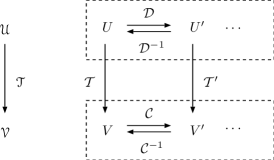
Figure 2: Two equivalence classes of unit systems (EUS’s) satisfying $\mathscr{U}\succ\mathscr{V}$, with the mapping $\mathscr{T}$. Each EUS contains equivalent unit systems as $\mathscr{U}=\{U,U^{\prime},\ldots\}$, $\mathscr{V}=\{V,V^{\prime},\ldots\}$. There are invertible mappings between any pair of unit systems in an EUS, for example, $\mathcal{D}$ and $\mathcal{D}^{-1}$ between $U$ and $U^{\prime}$. There is a (one-way) mapping from any unit system in $\mathscr{U}$ to any unit system in $\mathscr{V}$. These mappings ($\mathcal{T}$ and $\mathcal{T}^{\prime}$ in this example) are related as $\mathcal{T}^{\prime}=\mathcal{C}\mathcal{T}\mathcal{D}^{-1}$. Note that there are also mappings between $U$ and $V^{\prime}$ ($\mathcal{D}=\mathcal{I}$) or $U^{\prime}$ and $V$ ($\mathcal{C}=\mathcal{I}$), which is not shown here.

V.3 Dimension of e-quantities

In this subsection, we explore the meaning of dimension in detail using the framework of EUS. Two quantities, $Q_{U}=q_{U}[Q]_{U}=q_{U}{\mathchoice{\mbox{\boldmath$u$}}{\mbox{\boldmath$u$}}{\mbox{\scriptsize\boldmath$u$}}{\mbox{\scriptsize\boldmath$u$}}}^{{\mathchoice{\mbox{\boldmath$d$}}{\mbox{\boldmath$d$}}{\mbox{\scriptsize\boldmath$d$}}{\mbox{\scriptsize\boldmath$d$}}}}$ and $P_{U}=p_{U}[P]_{U}=p_{U}{\mathchoice{\mbox{\boldmath$u$}}{\mbox{\boldmath$u$}}{\mbox{\scriptsize\boldmath$u$}}{\mbox{\scriptsize\boldmath$u$}}}^{{\mathchoice{\mbox{\boldmath$c$}}{\mbox{\boldmath$c$}}{\mbox{\scriptsize\boldmath$c$}}{\mbox{\scriptsize\boldmath$c$}}}}$, represented in $U$ are considered to have a same dimension, if they are represented by the same unit; $[Q]_{U}=[P]_{U}$, or ${\mathchoice{\mbox{\boldmath$d$}}{\mbox{\boldmath$d$}}{\mbox{\scriptsize\boldmath$d$}}{\mbox{\scriptsize\boldmath$d$}}}={\mathchoice{\mbox{\boldmath$c$}}{\mbox{\boldmath$c$}}{\mbox{\scriptsize\boldmath$c$}}{\mbox{\scriptsize\boldmath$c$}}}$. As long as we use only one unit system, dimension is just a synonym of unit. However, in another unit system $V\succ U$, $Q$ and $P$ might be represented by different units. Therefore, unlike commonly believed, dimension could be dependent on unit systems.

On the other hand, for an equivalent unit system $U^{\prime}\sim U$, $[Q]_{U^{\prime}}=[P]_{U^{\prime}}$ always follows from $[Q]_{U}=[P]_{U}$, and vice versa. Thus, we expect that the notion of dimension can be consistently extended to every unit system belonging to the EUS.

Let us begin with a unit system $U\in\mathscr{U}$ with base units ${\mathchoice{\mbox{\boldmath$u$}}{\mbox{\boldmath$u$}}{\mbox{\scriptsize\boldmath$u$}}{\mbox{\scriptsize\boldmath$u$}}}=(u_{1},u_{2},\ldots,u_{N})$. For each base unit $u_{i}$, we introduce a set $\mathsf{U}_{i}=\{s_{i}u_{i}|s_{i}\in\mathbb{R}_{+}\}$, which is a collection of units different only in sizes. Then, we make a unit system $U^{\prime}$ with ${\mathchoice{\mbox{\boldmath$u$}}{\mbox{\boldmath$u$}}{\mbox{\scriptsize\boldmath$u$}}{\mbox{\scriptsize\boldmath$u$}}}^{\prime}=(u^{\prime}_{1},u^{\prime}_{2},\ldots,u^{\prime}_{N})$, $u^{\prime}_{i}=s_{i}^{-1}u_{i}\in\mathsf{U}_{i}$ $(i=1,2,\ldots,N)$. Each base unit of $U^{\prime}$ is only different in size from the corresponding base unit of $U$. The mapping is $\mathcal{S}=({\mathchoice{\mbox{\boldmath$s$}}{\mbox{\boldmath$s$}}{\mbox{\scriptsize\boldmath$s$}}{\mbox{\scriptsize\boldmath$s$}}},I):U\rightarrow U^{\prime}$, ${\mathchoice{\mbox{\boldmath$s$}}{\mbox{\boldmath$s$}}{\mbox{\scriptsize\boldmath$s$}}{\mbox{\scriptsize\boldmath$s$}}}=(s_{1},s_{2},\ldots,s_{N})^{\mbox{\scriptsize T}}$. Therefore, $U^{\prime}$ is equivalent to $U$ and belongs to $\mathscr{U}$. A quantity $Q$ can be expressed as $Q_{U}=q_{U}{\mathchoice{\mbox{\boldmath$u$}}{\mbox{\boldmath$u$}}{\mbox{\scriptsize\boldmath$u$}}{\mbox{\scriptsize\boldmath$u$}}}^{{\mathchoice{\mbox{\boldmath$d$}}{\mbox{\boldmath$d$}}{\mbox{\scriptsize\boldmath$d$}}{\mbox{\scriptsize\boldmath$d$}}}}$ in $U$ and $Q_{U^{\prime}}=q_{U^{\prime}}{\mathchoice{\mbox{\boldmath$u$}}{\mbox{\boldmath$u$}}{\mbox{\scriptsize\boldmath$u$}}{\mbox{\scriptsize\boldmath$u$}}}^{\prime{\mathchoice{\mbox{\boldmath$d$}}{\mbox{\boldmath$d$}}{\mbox{\scriptsize\boldmath$d$}}{\mbox{\scriptsize\boldmath$d$}}}}$ in $U^{\prime}$, respectively, and $d$ is conserved under the scaling of units.

We can consider that two expressions $Q_{U}=q_{U}{\mathchoice{\mbox{\boldmath$u$}}{\mbox{\boldmath$u$}}{\mbox{\scriptsize\boldmath$u$}}{\mbox{\scriptsize\boldmath$u$}}}^{{\mathchoice{\mbox{\boldmath$d$}}{\mbox{\boldmath$d$}}{\mbox{\scriptsize\boldmath$d$}}{\mbox{\scriptsize\boldmath$d$}}}}$ and $Q_{U^{\prime}}=q_{U^{\prime}}{\mathchoice{\mbox{\boldmath$u$}}{\mbox{\boldmath$u$}}{\mbox{\scriptsize\boldmath$u$}}{\mbox{\scriptsize\boldmath$u$}}}^{\prime{\mathchoice{\mbox{\boldmath$d$}}{\mbox{\boldmath$d$}}{\mbox{\scriptsize\boldmath$d$}}{\mbox{\scriptsize\boldmath$d$}}}}$ have a common dimension ${\mathchoice{\mbox{\boldmath$U$}}{\mbox{\boldmath$U$}}{\mbox{\scriptsize\boldmath$U$}}{\mbox{\scriptsize\boldmath$U$}}}^{{\mathchoice{\mbox{\boldmath$d$}}{\mbox{\boldmath$d$}}{\mbox{\scriptsize\boldmath$d$}}{\mbox{\scriptsize\boldmath$d$}}}}=\prod_{i=1}^{N}\mathsf{U}_{i}^{d_{i}}$, where ${\mathchoice{\mbox{\boldmath$U$}}{\mbox{\boldmath$U$}}{\mbox{\scriptsize\boldmath$U$}}{\mbox{\scriptsize\boldmath$U$}}}=(\mathsf{U}_{1},\mathsf{U}_{2},\ldots,\mathsf{U}_{N})$ is the dimensional basis. For example, $U=(\text{MKS})$, ${\mathchoice{\mbox{\boldmath$u$}}{\mbox{\boldmath$u$}}{\mbox{\scriptsize\boldmath$u$}}{\mbox{\scriptsize\boldmath$u$}}}=({\mu\Omega\mathrm{m}},{\mu\Omega\mathrm{kg}},{\mu\Omega\mathrm{s}})$ and $U^{\prime}=(\text{CGS})$, ${\mathchoice{\mbox{\boldmath$u$}}{\mbox{\boldmath$u$}}{\mbox{\scriptsize\boldmath$u$}}{\mbox{\scriptsize\boldmath$u$}}}^{\prime}=({\mu\Omega\mathrm{cm}},{\mu\Omega\mathrm{g}},{\mu\Omega\mathrm{s}})$ share the dimension of the form $\mathsf{L}^{l}\mathsf{M}^{m}\mathsf{T}^{t}$, since ${\mu\Omega\mathrm{cm}}=10^{-2}\,{\mu\Omega\mathrm{m}}\in\mathsf{L}$, ${\mu\Omega\mathrm{g}}=10^{-3}\,{\mu\Omega\mathrm{kg}}\in\mathsf{M}$, and ${\mu\Omega\mathrm{s}}\in\mathsf{T}$.

More generally, for any $U^{\prime}\in\mathscr{U}$, there exists an invertible mapping $\mathcal{D}=({\mathchoice{\mbox{\boldmath$k$}}{\mbox{\boldmath$k$}}{\mbox{\scriptsize\boldmath$k$}}{\mbox{\scriptsize\boldmath$k$}}},D):U\rightarrow U^{\prime}$ and ${\mathchoice{\mbox{\boldmath$U$}}{\mbox{\boldmath$U$}}{\mbox{\scriptsize\boldmath$U$}}{\mbox{\scriptsize\boldmath$U$}}}^{{\mathchoice{\mbox{\boldmath$d$}}{\mbox{\boldmath$d$}}{\mbox{\scriptsize\boldmath$d$}}{\mbox{\scriptsize\boldmath$d$}}}}={\mathchoice{\mbox{\boldmath$U$}}{\mbox{\boldmath$U$}}{\mbox{\scriptsize\boldmath$U$}}{\mbox{\scriptsize\boldmath$U$}}}^{\prime{\mathchoice{\mbox{\boldmath$d$}}{\mbox{\boldmath$d$}}{\mbox{\scriptsize\boldmath$d$}}{\mbox{\scriptsize\boldmath$d$}}}^{\prime}}$ holds, where

$${\mathchoice{\mbox{\boldmath$d$}}{\mbox{\boldmath$d$}}{\mbox{\scriptsize\boldmath$d$}}{\mbox{\scriptsize\boldmath$d$}}}^{\prime}=D{\mathchoice{\mbox{\boldmath$d$}}{\mbox{\boldmath$d$}}{\mbox{\scriptsize\boldmath$d$}}{\mbox{\scriptsize\boldmath$d$}}},\quad{\mathchoice{\mbox{\boldmath$U$}}{\mbox{\boldmath$U$}}{\mbox{\scriptsize\boldmath$U$}}{\mbox{\scriptsize\boldmath$U$}}}^{\prime}={\mathchoice{\mbox{\boldmath$U$}}{\mbox{\boldmath$U$}}{\mbox{\scriptsize\boldmath$U$}}{\mbox{\scriptsize\boldmath$U$}}}^{D^{-1}}.$$ (13)

As for dimensions, the scale factor $k$ plays no role. Under the transformation by any regular matrix $D$, the dimension ${\mathchoice{\mbox{\boldmath$U$}}{\mbox{\boldmath$U$}}{\mbox{\scriptsize\boldmath$U$}}{\mbox{\scriptsize\boldmath$U$}}}^{{\mathchoice{\mbox{\boldmath$d$}}{\mbox{\boldmath$d$}}{\mbox{\scriptsize\boldmath$d$}}{\mbox{\scriptsize\boldmath$d$}}}}$ is invariant, while $U$ and $d$ transform in a reciprocal manner. Dimension is conserved under invertible transformations of unit systems. Dimension is invariant in the EUS, since any pair of unit systems in an EUS can be related by an invertible transformation. The dimension of an e-quantity in $\mathscr{U}$ can be represented collectively as

$$[Q]_{\mathscr{U}}={\mathchoice{\mbox{\boldmath$U$}}{\mbox{\boldmath$U$}}{\mbox{\scriptsize\boldmath$U$}}{\mbox{\scriptsize\boldmath$U$}}}^{{\mathchoice{\mbox{\boldmath$d$}}{\mbox{\boldmath$d$}}{\mbox{\scriptsize\boldmath$d$}}{\mbox{\scriptsize\boldmath$d$}}}}={\mathchoice{\mbox{\boldmath$U$}}{\mbox{\boldmath$U$}}{\mbox{\scriptsize\boldmath$U$}}{\mbox{\scriptsize\boldmath$U$}}}^{\prime{\mathchoice{\mbox{\boldmath$d$}}{\mbox{\boldmath$d$}}{\mbox{\scriptsize\boldmath$d$}}{\mbox{\scriptsize\boldmath$d$}}}^{\prime}}=\cdots.$$ (14)

We consider an EUS $\mathscr{V}$ that is not equivalent to $\mathscr{U}$. The dimension of an e-quantity $Q_{\mathscr{V}}$ is expressed as $[Q]_{\mathscr{V}}={\mathchoice{\mbox{\boldmath$V$}}{\mbox{\boldmath$V$}}{\mbox{\scriptsize\boldmath$V$}}{\mbox{\scriptsize\boldmath$V$}}}^{{\mathchoice{\mbox{\boldmath$c$}}{\mbox{\boldmath$c$}}{\mbox{\scriptsize\boldmath$c$}}{\mbox{\scriptsize\boldmath$c$}}}}$ with ${\mathchoice{\mbox{\boldmath$V$}}{\mbox{\boldmath$V$}}{\mbox{\scriptsize\boldmath$V$}}{\mbox{\scriptsize\boldmath$V$}}}=(\mathsf{V}_{1},\mathsf{V}_{2},\ldots,\mathsf{V}_{M})$. If $\mathscr{U}\succ\mathscr{V}$, we have a non-invertible mapping $\mathcal{T}=({\mathchoice{\mbox{\boldmath$k$}}{\mbox{\boldmath$k$}}{\mbox{\scriptsize\boldmath$k$}}{\mbox{\scriptsize\boldmath$k$}}},T):U\in\mathscr{U}\rightarrow V\in\mathscr{V}$, by which we can convert the dimensions as $\mathcal{T}(\mathsf{U}_{i})={\mathchoice{\mbox{\boldmath$V$}}{\mbox{\boldmath$V$}}{\mbox{\scriptsize\boldmath$V$}}{\mbox{\scriptsize\boldmath$V$}}}^{{\mathchoice{\mbox{\boldmath$t$}}{\mbox{\boldmath$t$}}{\mbox{\scriptsize\boldmath$t$}}{\mbox{\scriptsize\boldmath$t$}}}_{i}}$ and ${\mathchoice{\mbox{\boldmath$c$}}{\mbox{\boldmath$c$}}{\mbox{\scriptsize\boldmath$c$}}{\mbox{\scriptsize\boldmath$c$}}}=T{\mathchoice{\mbox{\boldmath$d$}}{\mbox{\boldmath$d$}}{\mbox{\scriptsize\boldmath$d$}}{\mbox{\scriptsize\boldmath$d$}}}$, unidirectionally [See Eq. (6)]. Unlike the equivalent cases, the former equations cannot be expressed as ${\mathchoice{\mbox{\boldmath$V$}}{\mbox{\boldmath$V$}}{\mbox{\scriptsize\boldmath$V$}}{\mbox{\scriptsize\boldmath$V$}}}={\mathchoice{\mbox{\boldmath$U$}}{\mbox{\boldmath$U$}}{\mbox{\scriptsize\boldmath$U$}}{\mbox{\scriptsize\boldmath$U$}}}^{T^{-1}}$ because $T$ is not invertible. Therefore, we cannot equate ${\mathchoice{\mbox{\boldmath$U$}}{\mbox{\boldmath$U$}}{\mbox{\scriptsize\boldmath$U$}}{\mbox{\scriptsize\boldmath$U$}}}^{{\mathchoice{\mbox{\boldmath$d$}}{\mbox{\boldmath$d$}}{\mbox{\scriptsize\boldmath$d$}}{\mbox{\scriptsize\boldmath$d$}}}}$ and ${\mathchoice{\mbox{\boldmath$V$}}{\mbox{\boldmath$V$}}{\mbox{\scriptsize\boldmath$V$}}{\mbox{\scriptsize\boldmath$V$}}}^{{\mathchoice{\mbox{\boldmath$c$}}{\mbox{\boldmath$c$}}{\mbox{\scriptsize\boldmath$c$}}{\mbox{\scriptsize\boldmath$c$}}}}$. In the case of $\mathscr{U}\parallel\mathscr{V}$, there even exist no such direct relations between their dimensions. Some examples on dimension in EUS will be given in Sec. IX.G.

V.4 Dimensional analysis and the Buckingham Pi-theorem

The central result of dimensional analysis is the Buckingham Pi-theorembuckingham ; bridgman ; bluman . It imposes restrictions on the form of equations that are physically sensible. It also helps to extract non-dimensional parameters that characterizes the problem under consideration.

We outline the proof of the theorem in the framework of equivalence unit systems. Let us consider a set of e-quantities $P_{0},P_{1},P_{2},\ldots,P_{L}$ in $\mathscr{U}$ with $L>N:=\#\mathscr{U}$. We suppose they are related by a function $f$ as

$$P_{0}=f(P_{1},P_{2},\ldots,P_{L}).$$ (15)

For simplicity, we omit subscripts $\mathscr{U}$ in e-quantities in this subsection. We assume that these e-quantities are arranged so that $P_{1},P_{2},\ldots,P_{N}$ are dimensionally independent each other and $P_{0},P_{N+1},\ldots,P_{L}$ dependent on $P_{1},P_{2},\ldots,P_{N}$. We express the corresponding quantities in $U\in\mathscr{U}$ as $P_{l}=p_{lU}{\mathchoice{\mbox{\boldmath$u$}}{\mbox{\boldmath$u$}}{\mbox{\scriptsize\boldmath$u$}}{\mbox{\scriptsize\boldmath$u$}}}^{{\mathchoice{\mbox{\boldmath$d$}}{\mbox{\boldmath$d$}}{\mbox{\scriptsize\boldmath$d$}}{\mbox{\scriptsize\boldmath$d$}}}_{l}}$ $(l=0,1,\ldots,L)$. In terms of dimensional exponents in $U$, ${\mathchoice{\mbox{\boldmath$d$}}{\mbox{\boldmath$d$}}{\mbox{\scriptsize\boldmath$d$}}{\mbox{\scriptsize\boldmath$d$}}}_{1},{\mathchoice{\mbox{\boldmath$d$}}{\mbox{\boldmath$d$}}{\mbox{\scriptsize\boldmath$d$}}{\mbox{\scriptsize\boldmath$d$}}}_{2},\ldots,{\mathchoice{\mbox{\boldmath$d$}}{\mbox{\boldmath$d$}}{\mbox{\scriptsize\boldmath$d$}}{\mbox{\scriptsize\boldmath$d$}}}_{N}$ are linearly independents and ${\mathchoice{\mbox{\boldmath$d$}}{\mbox{\boldmath$d$}}{\mbox{\scriptsize\boldmath$d$}}{\mbox{\scriptsize\boldmath$d$}}}_{0},{\mathchoice{\mbox{\boldmath$d$}}{\mbox{\boldmath$d$}}{\mbox{\scriptsize\boldmath$d$}}{\mbox{\scriptsize\boldmath$d$}}}_{N+1},\ldots{\mathchoice{\mbox{\boldmath$d$}}{\mbox{\boldmath$d$}}{\mbox{\scriptsize\boldmath$d$}}{\mbox{\scriptsize\boldmath$d$}}}_{L}$ are linearly dependent on them, i.e.,

$${\mathchoice{\mbox{\boldmath$d$}}{\mbox{\boldmath$d$}}{\mbox{\scriptsize\boldmath$d$}}{\mbox{\scriptsize\boldmath$d$}}}_{k}=\sum_{n=1}^{N}{\mathchoice{\mbox{\boldmath$d$}}{\mbox{\boldmath$d$}}{\mbox{\scriptsize\boldmath$d$}}{\mbox{\scriptsize\boldmath$d$}}}_{n}T_{nk}=D{\mathchoice{\mbox{\boldmath$t$}}{\mbox{\boldmath$t$}}{\mbox{\scriptsize\boldmath$t$}}{\mbox{\scriptsize\boldmath$t$}}}_{k}\quad(k=0,N+1,\ldots,L),$$ (16)

where $D=[{\mathchoice{\mbox{\boldmath$d$}}{\mbox{\boldmath$d$}}{\mbox{\scriptsize\boldmath$d$}}{\mbox{\scriptsize\boldmath$d$}}}_{1},{\mathchoice{\mbox{\boldmath$d$}}{\mbox{\boldmath$d$}}{\mbox{\scriptsize\boldmath$d$}}{\mbox{\scriptsize\boldmath$d$}}}_{2},\ldots,{\mathchoice{\mbox{\boldmath$d$}}{\mbox{\boldmath$d$}}{\mbox{\scriptsize\boldmath$d$}}{\mbox{\scriptsize\boldmath$d$}}}_{N}]$ and ${\mathchoice{\mbox{\boldmath$t$}}{\mbox{\boldmath$t$}}{\mbox{\scriptsize\boldmath$t$}}{\mbox{\scriptsize\boldmath$t$}}}_{k}=(T_{1k},T_{2k},\ldots,T_{Nk})^{\mbox{\scriptsize T}}$. The coefficients $T_{nk}$ can be derived as ${\mathchoice{\mbox{\boldmath$t$}}{\mbox{\boldmath$t$}}{\mbox{\scriptsize\boldmath$t$}}{\mbox{\scriptsize\boldmath$t$}}}_{k}=D^{-1}{\mathchoice{\mbox{\boldmath$d$}}{\mbox{\boldmath$d$}}{\mbox{\scriptsize\boldmath$d$}}{\mbox{\scriptsize\boldmath$d$}}}_{k}$, once the dimensional exponents ${\mathchoice{\mbox{\boldmath$d$}}{\mbox{\boldmath$d$}}{\mbox{\scriptsize\boldmath$d$}}{\mbox{\scriptsize\boldmath$d$}}}_{l}$ $(l=0,1,\ldots,L)$ are given.

With these we can make dimensionless e-quantities by normalization as

$$\pi_{k}:=\frac{P_{k}}{{\mathchoice{\mbox{\boldmath$P$}}{\mbox{\boldmath$P$}}{\mbox{\scriptsize\boldmath$P$}}{\mbox{\scriptsize\boldmath$P$}}}^{{\mathchoice{\mbox{\boldmath$t$}}{\mbox{\boldmath$t$}}{\mbox{\scriptsize\boldmath$t$}}{\mbox{\scriptsize\boldmath$t$}}}_{k}}}\in\mathbb{R}\quad(k=0,N+1,\ldots,L),$$ (17)

where ${\mathchoice{\mbox{\boldmath$P$}}{\mbox{\boldmath$P$}}{\mbox{\scriptsize\boldmath$P$}}{\mbox{\scriptsize\boldmath$P$}}}=(P_{1},P_{2},\ldots,P_{N})$. Inserting into Eq. (15), we have

$$\pi_{0} ={\mathchoice{\mbox{\boldmath$P$}}{\mbox{\boldmath$P$}}{\mbox{\scriptsize\boldmath$P$}}{\mbox{\scriptsize\boldmath$P$}}}^{-{\mathchoice{\mbox{\boldmath$t$}}{\mbox{\boldmath$t$}}{\mbox{\scriptsize\boldmath$t$}}{\mbox{\scriptsize\boldmath$t$}}}_{0}}f(P_{1},P_{2},\ldots,P_{N},\pi_{N+1}{\mathchoice{\mbox{\boldmath$P$}}{\mbox{\boldmath$P$}}{\mbox{\scriptsize\boldmath$P$}}{\mbox{\scriptsize\boldmath$P$}}}^{{\mathchoice{\mbox{\boldmath$t$}}{\mbox{\boldmath$t$}}{\mbox{\scriptsize\boldmath$t$}}{\mbox{\scriptsize\boldmath$t$}}}_{N+1}},\ldots,\pi_{L}{\mathchoice{\mbox{\boldmath$P$}}{\mbox{\boldmath$P$}}{\mbox{\scriptsize\boldmath$P$}}{\mbox{\scriptsize\boldmath$P$}}}^{{\mathchoice{\mbox{\boldmath$t$}}{\mbox{\boldmath$t$}}{\mbox{\scriptsize\boldmath$t$}}{\mbox{\scriptsize\boldmath$t$}}}_{L}})$$

$$=F(P_{1},P_{2},\ldots,P_{N},\pi_{N+1},\ldots,\pi_{L}).$$ (18)

By introducing appropriate (non-dimensional) function $F$, we can absorb $P_{n}$’s in the normalization factors ${\mathchoice{\mbox{\boldmath$P$}}{\mbox{\boldmath$P$}}{\mbox{\scriptsize\boldmath$P$}}{\mbox{\scriptsize\boldmath$P$}}}^{{\mathchoice{\mbox{\boldmath$t$}}{\mbox{\boldmath$t$}}{\mbox{\scriptsize\boldmath$t$}}{\mbox{\scriptsize\boldmath$t$}}}_{k}}$ into the first $N$ arguments.

With ${\mathchoice{\mbox{\boldmath$P$}}{\mbox{\boldmath$P$}}{\mbox{\scriptsize\boldmath$P$}}{\mbox{\scriptsize\boldmath$P$}}}=(P_{1},P_{2},\ldots,P_{N})$, we can form a basis of unit system ${\mathchoice{\mbox{\boldmath$v$}}{\mbox{\boldmath$v$}}{\mbox{\scriptsize\boldmath$v$}}{\mbox{\scriptsize\boldmath$v$}}}=(v_{1},v_{2},\ldots,v_{N})$ in $\mathscr{U}$ by rescaling of $v_{n}=P_{n}/p_{nV}$ with arbitrary factors $p_{nV}\in\mathbb{R}_{+}$. In this unit system $V$, the numerical parts of $P_{n}$ and $\pi_{k}$ are $\{P_{n}\}_{V}=p_{nV}$ $(n=1,2,\ldots,N)$ and $\{\pi_{k}\}_{V}=\pi_{k}$ $(k=0,N+1,\ldots,L)$. Equation (18) should hold even if we replace the quantities with the corresponding numerical factors as

$$\pi_{0}=F(p_{1V},p_{2V},\ldots,p_{NV},\pi_{N+1},\ldots,\pi_{L}).$$ (19)

Since $p_{nV}$ can take any (positive) numerical values, the function $F$ should not depend on $p_{nV}$ and Eq. (19) reduces to a relation among the dimensionless parameters:

$$\pi_{0}=G(\pi_{n+1},\pi_{n+2},\ldots,\pi_{L}).$$ (20)

Thus the dimensional consideration helps to simplify the forms of physical equations.

VI Standard form of transformation

VI.1 Decomposition of the transfer matrix

For the case where $U\succsim V$ holds but $U\precsim V$ does not, i.e., the case of $U\succ V$, the mapping $\mathcal{T}=({\mathchoice{\mbox{\boldmath$k$}}{\mbox{\boldmath$k$}}{\mbox{\scriptsize\boldmath$k$}}{\mbox{\scriptsize\boldmath$k$}}},T)$ is not invertible. Then, $N>M$, and we set $L=N-M\geq 1$.

We can transform the matrix $T$ of rank $M$ into a standard form, $J=\left[I_{M}|0\right]$ with an $M\times M$ matrix $C$ and an $N\times N$ matrix $D$, both of which are invertible, as $T=C^{-1}JD$. The $M\times N$ matrix $J$ is composed of the $M\times M$ unit submatrix $I_{M}$ and the $M\times L$ zero submatrix maclane . Note that the matrix elements are all rational numbers.

We consider a series of mappings, $U\stackrel{{\scriptstyle\mathcal{D}}}{{\rightarrow}}U^{\prime}\stackrel{{\scriptstyle\mathcal{J}}}{{\rightarrow}}V^{\prime}\stackrel{{\scriptstyle\mathcal{C}^{-1}}}{{\rightarrow}}V$, where $U^{\prime}$ and $V^{\prime}$ are $N$-base and $M$-base unit systems, respectively. The invertible mappings are defined as $\mathcal{D}=({\mathchoice{\mbox{\boldmath$1$}}{\mbox{\boldmath$1$}}{\mbox{\scriptsize\boldmath$1$}}{\mbox{\scriptsize\boldmath$1$}}}_{N},D)$ and $\mathcal{C}=({\mathchoice{\mbox{\boldmath$1$}}{\mbox{\boldmath$1$}}{\mbox{\scriptsize\boldmath$1$}}{\mbox{\scriptsize\boldmath$1$}}}_{M},C)$. We also define a mapping $\mathcal{J}=({\mathchoice{\mbox{\boldmath$k$}}{\mbox{\boldmath$k$}}{\mbox{\scriptsize\boldmath$k$}}{\mbox{\scriptsize\boldmath$k$}}}^{\prime},J)$, in which ${\mathchoice{\mbox{\boldmath$k$}}{\mbox{\boldmath$k$}}{\mbox{\scriptsize\boldmath$k$}}{\mbox{\scriptsize\boldmath$k$}}}^{\prime}={\mathchoice{\mbox{\boldmath$k$}}{\mbox{\boldmath$k$}}{\mbox{\scriptsize\boldmath$k$}}{\mbox{\scriptsize\boldmath$k$}}}^{D^{-1}}$. Using Eqs. (9) and (10), we obtain the standard decomposition:

$$\mathcal{C}^{-1}\mathcal{J}\mathcal{D}=({\mathchoice{\mbox{\boldmath$1$}}{\mbox{\boldmath$1$}}{\mbox{\scriptsize\boldmath$1$}}{\mbox{\scriptsize\boldmath$1$}}}_{M}^{JD}{\mathchoice{\mbox{\boldmath$k$}}{\mbox{\boldmath$k$}}{\mbox{\scriptsize\boldmath$k$}}{\mbox{\scriptsize\boldmath$k$}}}^{\prime D}{\mathchoice{\mbox{\boldmath$1$}}{\mbox{\boldmath$1$}}{\mbox{\scriptsize\boldmath$1$}}{\mbox{\scriptsize\boldmath$1$}}}_{N},C^{-1}JD)=({\mathchoice{\mbox{\boldmath$k$}}{\mbox{\boldmath$k$}}{\mbox{\scriptsize\boldmath$k$}}{\mbox{\scriptsize\boldmath$k$}}},T)=\mathcal{T}.$$ (21)

VI.2 Quantities transferred to unity

The vectors ${\mathchoice{\mbox{\boldmath$d$}}{\mbox{\boldmath$d$}}{\mbox{\scriptsize\boldmath$d$}}{\mbox{\scriptsize\boldmath$d$}}}^{\prime}_{h}={\mathchoice{\mbox{\boldmath$e$}}{\mbox{\boldmath$e$}}{\mbox{\scriptsize\boldmath$e$}}{\mbox{\scriptsize\boldmath$e$}}}_{M+h}$ $(h=1,\ldots,L)$ belong to ${\rm ker}\,J$ and satisfy $J{\mathchoice{\mbox{\boldmath$d$}}{\mbox{\boldmath$d$}}{\mbox{\scriptsize\boldmath$d$}}{\mbox{\scriptsize\boldmath$d$}}}^{\prime}_{h}=0$, where ${\mathchoice{\mbox{\boldmath$e$}}{\mbox{\boldmath$e$}}{\mbox{\scriptsize\boldmath$e$}}{\mbox{\scriptsize\boldmath$e$}}}_{i}\in\mathbb{Q}^{N}$ is the $i$-th unit vector. Here, ${\rm ker}\,J$ represents the zero space (kernel) of $J$, i.e., the subspace spanned by the vectors ${\mathchoice{\mbox{\boldmath$d$}}{\mbox{\boldmath$d$}}{\mbox{\scriptsize\boldmath$d$}}{\mbox{\scriptsize\boldmath$d$}}}^{\prime}$ with $J{\mathchoice{\mbox{\boldmath$d$}}{\mbox{\boldmath$d$}}{\mbox{\scriptsize\boldmath$d$}}{\mbox{\scriptsize\boldmath$d$}}}^{\prime}=0$. Then, the vectors ${\mathchoice{\mbox{\boldmath$d$}}{\mbox{\boldmath$d$}}{\mbox{\scriptsize\boldmath$d$}}{\mbox{\scriptsize\boldmath$d$}}}_{h}=D^{-1}{\mathchoice{\mbox{\boldmath$d$}}{\mbox{\boldmath$d$}}{\mbox{\scriptsize\boldmath$d$}}{\mbox{\scriptsize\boldmath$d$}}}^{\prime}_{h}$ belong to ${\rm ker}\,T$ and satisfy $T{\mathchoice{\mbox{\boldmath$d$}}{\mbox{\boldmath$d$}}{\mbox{\scriptsize\boldmath$d$}}{\mbox{\scriptsize\boldmath$d$}}}_{h}=0$.

Using ${\mathchoice{\mbox{\boldmath$d$}}{\mbox{\boldmath$d$}}{\mbox{\scriptsize\boldmath$d$}}{\mbox{\scriptsize\boldmath$d$}}}_{h}$, we can define the following representations in $U$:

$$I_{hU}={\mathchoice{\mbox{\boldmath$k$}}{\mbox{\boldmath$k$}}{\mbox{\scriptsize\boldmath$k$}}{\mbox{\scriptsize\boldmath$k$}}}^{-{\mathchoice{\mbox{\boldmath$d$}}{\mbox{\boldmath$d$}}{\mbox{\scriptsize\boldmath$d$}}{\mbox{\scriptsize\boldmath$d$}}}_{h}}{\mathchoice{\mbox{\boldmath$u$}}{\mbox{\boldmath$u$}}{\mbox{\scriptsize\boldmath$u$}}{\mbox{\scriptsize\boldmath$u$}}}^{{\mathchoice{\mbox{\boldmath$d$}}{\mbox{\boldmath$d$}}{\mbox{\scriptsize\boldmath$d$}}{\mbox{\scriptsize\boldmath$d$}}}_{h}},$$ (22)

which is mapped to $V$ by $\mathcal{T}$ as

$$I_{hV}=\mathcal{T}(I_{hU})={\mathchoice{\mbox{\boldmath$k$}}{\mbox{\boldmath$k$}}{\mbox{\scriptsize\boldmath$k$}}{\mbox{\scriptsize\boldmath$k$}}}^{-{\mathchoice{\mbox{\boldmath$d$}}{\mbox{\boldmath$d$}}{\mbox{\scriptsize\boldmath$d$}}{\mbox{\scriptsize\boldmath$d$}}}_{h}}{\mathchoice{\mbox{\boldmath$k$}}{\mbox{\boldmath$k$}}{\mbox{\scriptsize\boldmath$k$}}{\mbox{\scriptsize\boldmath$k$}}}^{{\mathchoice{\mbox{\boldmath$d$}}{\mbox{\boldmath$d$}}{\mbox{\scriptsize\boldmath$d$}}{\mbox{\scriptsize\boldmath$d$}}}_{h}}{\mathchoice{\mbox{\boldmath$v$}}{\mbox{\boldmath$v$}}{\mbox{\scriptsize\boldmath$v$}}{\mbox{\scriptsize\boldmath$v$}}}^{T{\mathchoice{\mbox{\boldmath$d$}}{\mbox{\boldmath$d$}}{\mbox{\scriptsize\boldmath$d$}}{\mbox{\scriptsize\boldmath$d$}}}_{h}}=1{\mathchoice{\mbox{\boldmath$v$}}{\mbox{\boldmath$v$}}{\mbox{\scriptsize\boldmath$v$}}{\mbox{\scriptsize\boldmath$v$}}}^{0}=1.$$ (23)

Thus, the representations $I_{hU}$ ($h=1,2,\ldots,L$) are all considered to be unity in $V$. The corresponding e-quantities $I_{h\mathscr{U}}$ are also considered to be unity in $\mathscr{V}$.

If we have two e-quantities $Q_{1\mathscr{U}}$ and $Q_{2\mathscr{U}}$, which are related in $\mathscr{U}$ as $Q_{1\mathscr{U}}=I_{h\mathscr{U}}Q_{2\mathscr{U}}$, then $Q_{1\mathscr{U}}$ and $Q_{2\mathscr{U}}$ cannot be distinguished in $\mathscr{V}$ because of $I_{h\mathscr{V}}=1$.

More generally, the relation $Q_{1\mathscr{U}}=I_{1\mathscr{U}}^{d_{1}}\cdots I_{L\mathscr{U}}^{d_{L}}Q_{2\mathscr{U}}$ with $(d_{1},\ldots,d_{L})^{\mbox{\scriptsize T}}\in\mathbb{Q}^{L}$, reduces to $Q_{1\mathscr{V}}=Q_{2\mathscr{V}}$ in $\mathscr{V}$. Therefore, the mapping $\mathscr{T}:\mathscr{U}\rightarrow\mathscr{V}$ is characterized by the preimage $\mathscr{T}^{-1}(1)=\{I_{1\mathscr{U}}^{d_{1}}\cdots I_{L\mathscr{U}}^{d_{L}}\,|\,d_{1},\ldots,d_{L}\in\mathbb{Q}\}$.

Now we know the implications of a shorthand method, in which some quantities are considered to be unity, e.g., “we set $c_{0}=1$.”

VII Comparison of unit systems with normalized quantities

VII.1 Normalized quantities

As discussed earlier, we cannot directly equate the representations in non-equivalent unit systems, even if each representation corresponds to the same quantity. In order to overcome this inconvenience, we introduce the notion of normalization. We assume that $\mathscr{U}\succ\mathscr{V}$ and show that $\mathscr{V}$ can be embedded into $\mathscr{U}$ by appropriately normalizing each e-quantity.

We use the standard decomposition (21). In $U^{\prime}\in\mathscr{U}$, $I_{h\mathscr{U}}$ is simply represented as $I_{hU^{\prime}}={\mathchoice{\mbox{\boldmath$k$}}{\mbox{\boldmath$k$}}{\mbox{\scriptsize\boldmath$k$}}{\mbox{\scriptsize\boldmath$k$}}}^{-{\mathchoice{\mbox{\boldmath$d$}}{\mbox{\boldmath$d$}}{\mbox{\scriptsize\boldmath$d$}}{\mbox{\scriptsize\boldmath$d$}}}_{h}}{\mathchoice{\mbox{\boldmath$u$}}{\mbox{\boldmath$u$}}{\mbox{\scriptsize\boldmath$u$}}{\mbox{\scriptsize\boldmath$u$}}}^{\prime{\mathchoice{\mbox{\boldmath$d$}}{\mbox{\boldmath$d$}}{\mbox{\scriptsize\boldmath$d$}}{\mbox{\scriptsize\boldmath$d$}}}^{\prime}_{h}}=(k_{M+h}^{\prime})^{-1}u^{\prime}_{M+h}$. We have used Eq. (22) and ${\mathchoice{\mbox{\boldmath$k$}}{\mbox{\boldmath$k$}}{\mbox{\scriptsize\boldmath$k$}}{\mbox{\scriptsize\boldmath$k$}}}^{\prime{\mathchoice{\mbox{\boldmath$d$}}{\mbox{\boldmath$d$}}{\mbox{\scriptsize\boldmath$d$}}{\mbox{\scriptsize\boldmath$d$}}}^{\prime}_{h}}={\mathchoice{\mbox{\boldmath$k$}}{\mbox{\boldmath$k$}}{\mbox{\scriptsize\boldmath$k$}}{\mbox{\scriptsize\boldmath$k$}}}^{{\mathchoice{\mbox{\boldmath$d$}}{\mbox{\boldmath$d$}}{\mbox{\scriptsize\boldmath$d$}}{\mbox{\scriptsize\boldmath$d$}}}_{h}}$. For any $Q_{\mathscr{U}}$, which is represented as $Q_{U^{\prime}}=q_{U}{\mathchoice{\mbox{\boldmath$u$}}{\mbox{\boldmath$u$}}{\mbox{\scriptsize\boldmath$u$}}{\mbox{\scriptsize\boldmath$u$}}}^{\prime{\mathchoice{\mbox{\boldmath$d$}}{\mbox{\boldmath$d$}}{\mbox{\scriptsize\boldmath$d$}}{\mbox{\scriptsize\boldmath$d$}}}^{\prime}}$ in $U^{\prime}$, we introduce a representation $N_{U^{\prime}}(Q_{\mathscr{U}})=I_{1U^{\prime}}^{-d^{\prime}_{M+1}}\cdots I_{LU^{\prime}}^{-d^{\prime}_{M+L}}$, which satisfies $N_{V}(Q_{\mathscr{U}})=1$ and cancels the higher portion $(d^{\prime}_{M+1},\ldots,d^{\prime}_{M+L})$ of dimensional exponent of $Q_{U^{\prime}}$. Then, we define a normalized representation of $Q_{U}$ in $U^{\prime}$:

$$\tilde{Q}_{U^{\prime}}=N_{U^{\prime}}(Q_{\mathscr{U}})Q_{U}=q_{U}(k_{M+1}^{\prime})^{d_{M+1}^{\prime}}\cdots(k_{M+L}^{\prime})^{d_{M+L}^{\prime}}u_{1}^{\prime d^{\prime}_{1}}\cdots u_{M}^{\prime d^{\prime}_{M}}.$$ (24)

The normalized e-quantity $\tilde{Q}_{\mathscr{U}}=N(Q_{\mathscr{U}})Q_{\mathscr{U}}$ can be represented only by the subset of base units: $\tilde{{\mathchoice{\mbox{\boldmath$u$}}{\mbox{\boldmath$u$}}{\mbox{\scriptsize\boldmath$u$}}{\mbox{\scriptsize\boldmath$u$}}}}^{\prime}=(u_{1}^{\prime},\ldots,u_{M}^{\prime})\subset{\mathchoice{\mbox{\boldmath$u$}}{\mbox{\boldmath$u$}}{\mbox{\scriptsize\boldmath$u$}}{\mbox{\scriptsize\boldmath$u$}}}^{\prime}$. Owing to ${\mathchoice{\mbox{\boldmath$v$}}{\mbox{\boldmath$v$}}{\mbox{\scriptsize\boldmath$v$}}{\mbox{\scriptsize\boldmath$v$}}}^{\prime}=J{\mathchoice{\mbox{\boldmath$u$}}{\mbox{\boldmath$u$}}{\mbox{\scriptsize\boldmath$u$}}{\mbox{\scriptsize\boldmath$u$}}}^{\prime}$, $\tilde{{\mathchoice{\mbox{\boldmath$u$}}{\mbox{\boldmath$u$}}{\mbox{\scriptsize\boldmath$u$}}{\mbox{\scriptsize\boldmath$u$}}}}$ is faithfully mapped to ${\mathchoice{\mbox{\boldmath$v$}}{\mbox{\boldmath$v$}}{\mbox{\scriptsize\boldmath$v$}}{\mbox{\scriptsize\boldmath$v$}}}^{\prime}$: $v_{i}^{\prime}=\tilde{u}_{i}^{\prime}$ $(i=1,2,\ldots,M)$. This means that there is a one-to-one correspondence between $\tilde{Q}_{U^{\prime}}$ and $Q_{V^{\prime}}$, or between $\tilde{Q}_{\mathscr{U}}$ and $Q_{\mathscr{V}}$. The normalization $Q_{\mathscr{U}}\mapsto\tilde{Q}_{\mathscr{U}}=N_{\mathscr{U}}(Q_{\mathscr{U}})Q_{\mathscr{U}}$ is found to be equivalent to the mapping $\mathscr{T}:Q_{\mathscr{U}}\mapsto Q_{\mathscr{V}}$. Note that $\mathscr{T}(N_{\mathscr{U}}(Q_{\mathscr{U}}))=1$ for any $Q_{\mathscr{U}}$.

For $Q_{1\mathscr{U}}$ and $Q_{2\mathscr{U}}$, we can define the normalized e-quantities as $\tilde{Q}_{1\mathscr{U}}=N_{\mathscr{U}}(Q_{1\mathscr{U}})Q_{1\mathscr{U}}$ and $\tilde{Q}_{2\mathscr{U}}=N_{\mathscr{U}}(Q_{2\mathscr{U}})Q_{2\mathscr{U}}$. It is possible to render a situation in which $\tilde{Q}_{1\mathscr{U}}=\tilde{Q}_{2\mathscr{U}}$ and $Q_{1\mathscr{U}}\neq Q_{2\mathscr{U}}$ in $\mathscr{U}$. Thanks to the normalization factors $N_{\mathscr{U}}(Q_{\mathscr{U}})$, we can keep track of the difference.

For the situation in which we need to clarify the unit system $V$ to which we move, we write $\tilde{Q}_{U}^{V}=N_{U}^{V}(Q)Q_{U}$, and the same for the EUS, $\tilde{Q}_{\mathscr{U}}^{\mathscr{V}}=N_{\mathscr{U}}^{\mathscr{V}}(Q)Q_{\mathscr{U}}$.

VII.2 Comparison of incomparable unit systems

We now consider the situation in which we have to compare unit systems $U$ and $V$, which are incomparable, i.e., $U\parallel V$. These unit systems cannot be compared directly because, in $U$ and $V$, the quantities are classified with different principles. The normalization method only works for $U\succsim V$ or $U\precsim V$. Fortunately, we can handle this situation by finding a unit system $W$ that is transferable to both $U$ and $V$, i.e., $W\succsim U$ and $W\succsim V$. Then, we can normalize quantities as $\tilde{Q}_{W}^{U}=N_{W}^{U}(Q)Q_{W}$ and $\tilde{Q}_{W}^{V}=N_{W}^{V}(Q)Q_{W}$.

Thus, the representation in $U$ and $V$ can be embedded into $W$ and can be considered as representations in $W$.

VIII Practical Unit Systems

Historically, a number of types of unit systems have been proposed and adopted but, at present, only a few of them are used gupta . This is partly because the use of the International System of Units (SI) si , which is an extended version of the MKSA system, is strongly recommended and has gained popularity. Even though a systematic study of unit systems may no longer appear to be necessary, we sometimes need to read articles and books that are based on old unit systems and to convert quantities from one unit system to another. On such occasions, although conversion tables can be used, there is no reliable way to confirm the correctness of the conversion. Therefore, we need to have a rigorous theory of unit systems so that we can confirm the accuracy of conversion tables in textbooks. We can also logically assess presently used unit systems and compare them to systems that may be developed in the future.

In the this article, we deal with several electromagnetic unit systems as examples. The MKSA system, or the electromagnetic subset of the SI, is a four-base unit system. Hereafter, we use the terms MKSA and SI interchangeably. The CGS emu (electromagnetic unit) system and the CGS eus (electrostatic unit) system are both three-base unit systems maxwell2 . Normally, people use the non-rationalized versions of these systems in order to simplify (or to remove the factor $4\pi$ from) the Coulomb and Biot-Savard laws. However, the present consensus is that the rationalized system, in which the factor $4\pi$ is moved to the field solutions for point sources, is more reasonable. Therefore, in the present article, in order to simplify the argument, we use only rationalized systems and denote these systems as rCGS-emu (emu for short) and rCGS-esu (esu).

The CGS Gaussian system is a mixture of the CGS-emu and CGS-esu systems birge ; jackson ; kitano . We deal with only its rationalized version, which is referred to as the Heaviside-Lorentz (HL) system sommerfeld . Moreover, we have to introduce a variant jackson , which is modified to correct a defect of the HL system as explained later. We hereafter refer to this version as the modified Heaviside-Lorentz system (mHL).

VIII.1 Examples of the use of normalized quantities

As emphasized repeatedly, we should be very careful not to equate representations in different unit systems, such as $Q_{U}=Q_{V}$. In the following, we further explore this point because, although subtle, this is an important consideration. The unit of electric current in the MKSA (or SI), $I_{\mbox{\scriptsize SI}}=1\,{\mu\Omega\mathrm{A}}$, is represented in the rCGS-emu as $I_{\mbox{\scriptsize emu}}=\sqrt{4\pi}\times 10^{-1}\,{\mu\Omega\mathrm{\sqrt{dyn}}}$ jackson . Even then, we should not write $I_{\mbox{\scriptsize SI}}=I_{\mbox{\scriptsize emu}}$, because $1\,{\mu\Omega\mathrm{A}}=\sqrt{4\pi}\times 10^{-1}\,{\mu\Omega\mathrm{\sqrt{dyn}}}$ is dimensionally inconsistent. From the viewpoint of rCGS-emu, the left-hand side contains an undefined unit, “A”. From the viewpoint of MKSA, the equation reduces to $1\,{\mu\Omega\mathrm{A}}=\sqrt{40\pi}\times 10^{-3}\,{\mu\Omega\mathrm{\sqrt{N}}}$, which is incorrect.

Let us consider this problem in more detail. Since $I_{\mbox{\scriptsize SI}}/{\mu\Omega\mathrm{A}}=1$ and $I_{\mbox{\scriptsize emu}}/{\mu\Omega\mathrm{\sqrt{dyn}}}=\sqrt{4\pi}/10$, we obtain the following dimensionless relation:

$$\frac{I_{\mbox{\scriptsize emu}}}{{\mu\Omega\mathrm{\sqrt{dyn}}}}=\frac{\sqrt{4\pi}}{10}\frac{I_{\mbox{\scriptsize SI}}}{{\mu\Omega\mathrm{A}}},$$ (25)

which is valid for current of any amplitude. This is the best we can do for representations of different unit systems. We cannot multiply both sides by ${\mu\Omega\mathrm{\sqrt{dyn}}}$ or by ${\mu\Omega\mathrm{A}}$ in order to simplify the equations. In the former case, we have a mixture of units on the right-hand side, and in the latter case, we have a mixture of units on the left-hand side. In order to proceed, we can use the normalization and have a relation in the MKSA,

$$\tilde{I}^{\mbox{\scriptsize emu}}_{\mbox{\scriptsize SI}}=\sqrt{\rule{0.0pt}{5.59721pt}\mu_{\mbox{\scriptsize$0$,SI}}}I_{\mbox{\scriptsize SI}},$$ (26)

which corresponds to Eq. (25). Using $\tilde{I}^{\mbox{\scriptsize emu}}_{\mbox{\scriptsize SI}}$ instead of $I_{\mbox{\scriptsize emu}}$, we can legitimately multiply both sides by $\sqrt{{\mu\Omega\mathrm{dyn}}}=\sqrt{10^{-5}\,{\mu\Omega\mathrm{N}}}$. Note that $\mu_{\mbox{\scriptsize$0$,SI}}=4\pi\times 10^{-7}\,{\mu\Omega\mathrm{N/A^{2}}}$.

As another example, we consider a magnetic field strength $H$ and a magnetic flux density $B$, each of which are represented in the MKSA and rCGSemu. If the relation

$$B_{\mbox{\scriptsize SI}}=\mu_{\mbox{\scriptsize$0$,SI}}H_{\mbox{\scriptsize SI}},$$ (27)

is satisfied in the MKSA, then, in the rCGSemu,

$$B_{\mbox{\scriptsize emu}}=H_{\mbox{\scriptsize emu}},$$ (28)

holds. If we mistakenly write $B_{\mbox{\scriptsize SI}}=B_{\mbox{\scriptsize emu}}$ and $H_{\mbox{\scriptsize SI}}=H_{\mbox{\scriptsize emu}}$, then we have a contradictory relation $\mu_{\mbox{\scriptsize$0$,SI}}=1$.

Using the normalization $\tilde{B}^{\mbox{\scriptsize emu}}_{\mbox{\scriptsize SI}}:=(1/\sqrt{\rule{0.0pt}{5.59721pt}\mu_{\mbox{\scriptsize$0$,SI}}})B_{\mbox{\scriptsize SI}}$, $\tilde{H}^{\mbox{\scriptsize emu}}_{\mbox{\scriptsize SI}}:=\sqrt{\rule{0.0pt}{5.59721pt}\mu_{\mbox{\scriptsize$0$,SI}}}H_{\mbox{\scriptsize SI}}$, we have $\tilde{B}^{\mbox{\scriptsize emu}}_{\mbox{\scriptsize SI}}=\tilde{H}^{\mbox{\scriptsize emu}}_{\mbox{\scriptsize SI}}$, which corresponds to Eq. (28). Similarly, for the rCGS-esu, $\tilde{B}^{\mbox{\scriptsize esu}}_{\mbox{\scriptsize SI}}:=\sqrt{\rule{0.0pt}{5.59721pt}\varepsilon_{\mbox{\scriptsize$0$,SI}}}B_{\mbox{\scriptsize SI}}$, $\tilde{H}^{\mbox{\scriptsize esu}}_{\mbox{\scriptsize SI}}:=(1/\sqrt{\rule{0.0pt}{5.59721pt}\varepsilon_{\mbox{\scriptsize$0$,SI}}})H_{\mbox{\scriptsize SI}}$, we have $\tilde{B}^{\mbox{\scriptsize esu}}_{\mbox{\scriptsize SI}}=(1/c_{0,SI}^{2})\tilde{H}^{\mbox{\scriptsize esu}}_{\mbox{\scriptsize SI}}$.

The next example is to compare the representation of a charge in the esu and emu. We have $\tilde{q}^{\mbox{\scriptsize esu}}_{\mbox{\scriptsize SI}}=q_{\mbox{\scriptsize SI}}/\sqrt{\varepsilon_{\mbox{\scriptsize 0SI}}}$ and $\tilde{q}^{\mbox{\scriptsize emu}}_{\mbox{\scriptsize SI}}=\sqrt{\mu_{\mbox{\scriptsize 0SI}}}q_{\mbox{\scriptsize SI}}$, the units of which are ${\mu\Omega\mathrm{\sqrt{N}\,m}}$ and ${\mu\Omega\mathrm{\sqrt{N}\,s}}$, respectively. From these we obtain the notable Weber-Kohlrausch relation maxwell2 as follows: $\tilde{q}^{\mbox{\scriptsize esu}}_{\mbox{\scriptsize SI}}/\tilde{q}^{\mbox{\scriptsize emu}}_{\mbox{\scriptsize SI}}=c_{\mbox{\scriptsize 0SI}}$. Thus the MKSA system serves as a framework for comparing the rCGS-emu and rCGS-esu systems.

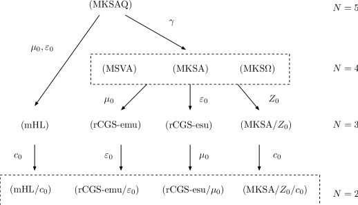
Figure 3: A hierarchical tree of unit systems. Here, $N$ is the number of base units. Arrows indicate transferability “$\succ$”, and the associated quantity is considered to be unity on the transfer. Dashed boxes represent EUS’s, and the four- and two-base unit systems listed are equivalent within each group, whereas the three-base unit systems are all incomparable.

IX Relations between real unit systems

In the following, we compare several unit systems, some of which are practically used systems.

IX.1 Example 1

Let us start with a toy model. We consider a set $\varOmega$, which includes quantities for voltage and current. In a unit system $U$, we use the ampere and the volt as the base units, ${\mathchoice{\mbox{\boldmath$u$}}{\mbox{\boldmath$u$}}{\mbox{\scriptsize\boldmath$u$}}{\mbox{\scriptsize\boldmath$u$}}}=({\mu\Omega\mathrm{A}},{\mu\Omega\mathrm{V}})$, and in the other system $V$, the watt and the ohm, ${\mathchoice{\mbox{\boldmath$v$}}{\mbox{\boldmath$v$}}{\mbox{\scriptsize\boldmath$v$}}{\mbox{\scriptsize\boldmath$v$}}}=({\mu\Omega\mathrm{W}},{\mu\Omega\mathrm{O}})$. We have $\mathcal{T}({\mu\Omega\mathrm{A}})=1\,{\mu\Omega\mathrm{W^{1/2}O^{-1/2}}}$, $\mathcal{T}({\mu\Omega\mathrm{V}})=1\,{\mu\Omega\mathrm{W^{1/2}O^{1/2}}}$, and find $\mathcal{T}=({\mathchoice{\mbox{\boldmath$k$}}{\mbox{\boldmath$k$}}{\mbox{\scriptsize\boldmath$k$}}{\mbox{\scriptsize\boldmath$k$}}},T):U\rightarrow V$ as

$${\mathchoice{\mbox{\boldmath$k$}}{\mbox{\boldmath$k$}}{\mbox{\scriptsize\boldmath$k$}}{\mbox{\scriptsize\boldmath$k$}}}=(1,1),\quad T=\begin{bmatrix}1/2&1/2\\ -1/2&1/2\end{bmatrix}.$$ (29)

We see that $\text{ker}\,T=\{0\}$, i.e., $\mathcal{T}$ is invertible, and $U\sim V$.

IX.2 Example 2

As another simple example, we consider a set $\varOmega$, which includes quantities for time and length. In $U$, we adopt the base units ${\mathchoice{\mbox{\boldmath$u$}}{\mbox{\boldmath$u$}}{\mbox{\scriptsize\boldmath$u$}}{\mbox{\scriptsize\boldmath$u$}}}=({\mu\Omega\mathrm{m}},{\mu\Omega\mathrm{s}})$ and in $V$ we use ${\mathchoice{\mbox{\boldmath$v$}}{\mbox{\boldmath$v$}}{\mbox{\scriptsize\boldmath$v$}}{\mbox{\scriptsize\boldmath$v$}}}=({\mu\Omega\mathrm{m}})$. In the latter, time is measured in terms of length with the help of the speed of light $c_{0}$. We have $\mathcal{T}({\mu\Omega\mathrm{m}})=1\,{\mu\Omega\mathrm{m}}$, $\mathcal{T}({\mu\Omega\mathrm{s}})=\{c_{0}\}_{U}\,{\mu\Omega\mathrm{m}}$, where $\{c_{0}\}_{U}:=c_{0U}/({\mu\Omega\mathrm{m/s}})=299\,792\,458$. Then we obtain

$${\mathchoice{\mbox{\boldmath$k$}}{\mbox{\boldmath$k$}}{\mbox{\scriptsize\boldmath$k$}}{\mbox{\scriptsize\boldmath$k$}}}=(1,\,\{c_{0}\}_{U}),\quad T=\begin{bmatrix}1&1\end{bmatrix}.$$ (30)

We see that $U\succ V$. From ${\mathchoice{\mbox{\boldmath$d$}}{\mbox{\boldmath$d$}}{\mbox{\scriptsize\boldmath$d$}}{\mbox{\scriptsize\boldmath$d$}}}_{1}=(1,-1)^{\mbox{\scriptsize T}}\in{\rm ker}\,T$, we have $I_{1U}={\mathchoice{\mbox{\boldmath$k$}}{\mbox{\boldmath$k$}}{\mbox{\scriptsize\boldmath$k$}}{\mbox{\scriptsize\boldmath$k$}}}^{-{\mathchoice{\mbox{\boldmath$d$}}{\mbox{\boldmath$d$}}{\mbox{\scriptsize\boldmath$d$}}{\mbox{\scriptsize\boldmath$d$}}}_{1}}{\mathchoice{\mbox{\boldmath$u$}}{\mbox{\boldmath$u$}}{\mbox{\scriptsize\boldmath$u$}}{\mbox{\scriptsize\boldmath$u$}}}^{{\mathchoice{\mbox{\boldmath$d$}}{\mbox{\boldmath$d$}}{\mbox{\scriptsize\boldmath$d$}}{\mbox{\scriptsize\boldmath$d$}}}_{1}}=\{c_{0}\}_{U}\,{\mu\Omega\mathrm{m}}\,{\mu\Omega\mathrm{s}}^{-1}=c_{0U}$ in $U$, which is mapped to $I_{1V}=c_{0V}=1$ in $V$. This corresponds to the first step toward natural unit systems duff . This procedure is sometimes written shortly as “we set $c_{0}=1$.”

IX.3 MKSA to CGS emu

Next, we examine a more practical example. We consider $U=(\text{MKSA})$ and $V=(\text{rCGS emu})$. The base units are ${\mathchoice{\mbox{\boldmath$u$}}{\mbox{\boldmath$u$}}{\mbox{\scriptsize\boldmath$u$}}{\mbox{\scriptsize\boldmath$u$}}}=({\mu\Omega\mathrm{m}},{\mu\Omega\mathrm{kg}},{\mu\Omega\mathrm{s}},{\mu\Omega\mathrm{A}})$ and ${\mathchoice{\mbox{\boldmath$v$}}{\mbox{\boldmath$v$}}{\mbox{\scriptsize\boldmath$v$}}{\mbox{\scriptsize\boldmath$v$}}}=({\mu\Omega\mathrm{cm}},{\mu\Omega\mathrm{g}},{\mu\Omega\mathrm{s}})$, respectively. Clearly, we have $\mathcal{T}({\mu\Omega\mathrm{m}})=100\,{\mu\Omega\mathrm{cm}}$, and $\mathcal{T}({\mu\Omega\mathrm{kg}})=1000\,{\mu\Omega\mathrm{g}}$. Using the relation jackson :

$$\frac{I_{\mbox{\scriptsize emu}}}{{\mu\Omega\mathrm{\sqrt{dyn}}}}=\frac{\sqrt{4\pi}}{10}\frac{I_{\mbox{\scriptsize SI}}}{{\mu\Omega\mathrm{A}}},$$ (31)

or $\mathcal{T}({\mu\Omega\mathrm{A}})=\sqrt{4\pi}10^{-1}\,{\mu\Omega\mathrm{cm^{1/2}g^{1/2}s^{-1}}}$, we obtain

$${\mathchoice{\mbox{\boldmath$k$}}{\mbox{\boldmath$k$}}{\mbox{\scriptsize\boldmath$k$}}{\mbox{\scriptsize\boldmath$k$}}}=(100,\,1000,\,1,\,\sqrt{4\pi}/10),\quad T=\begin{bmatrix}1&0&0&1/2\\ 0&1&0&1/2\\ 0&0&1&-1\end{bmatrix}.$$ (32)

Clearly, we have $U\succ V$. With ${\mathchoice{\mbox{\boldmath$d$}}{\mbox{\boldmath$d$}}{\mbox{\scriptsize\boldmath$d$}}{\mbox{\scriptsize\boldmath$d$}}}_{1}=(1,1,-2,-2)^{\mbox{\scriptsize T}}\in{\rm ker}\,T$, the representation

$$I_{1U}=100^{-1}\times 1000^{-1}\times 4\pi\times 10^{-2}\,{\mu\Omega\mathrm{m\,kg\,s^{-2}\,A^{-2}}}=4\pi\times 10^{-7}\,{\mu\Omega\mathrm{N/A^{2}}}=\mu_{0U},$$ (33)

in $U$ is identified with $\mu_{0V}=1$ in $V$.

IX.4 MKSA to CGS esu

Similarly, we consider $U=(\text{MKSA})$ and $V=(\text{rCGS esu})$. The base units are ${\mathchoice{\mbox{\boldmath$u$}}{\mbox{\boldmath$u$}}{\mbox{\scriptsize\boldmath$u$}}{\mbox{\scriptsize\boldmath$u$}}}=({\mu\Omega\mathrm{m}},{\mu\Omega\mathrm{kg}},{\mu\Omega\mathrm{s}},{\mu\Omega\mathrm{A}})$, ${\mathchoice{\mbox{\boldmath$v$}}{\mbox{\boldmath$v$}}{\mbox{\scriptsize\boldmath$v$}}{\mbox{\scriptsize\boldmath$v$}}}=({\mu\Omega\mathrm{cm}},{\mu\Omega\mathrm{g}},{\mu\Omega\mathrm{s}})$. Using the relation jackson

$$\frac{I_{\mbox{\scriptsize esu}}}{{\mu\Omega\mathrm{\sqrt{dyn}\cdot cm/s}}}=\sqrt{4\pi}\times 10\times\{c_{0}\}_{U}\frac{I_{\mbox{\scriptsize SI}}}{{\mu\Omega\mathrm{A}}},$$ (34)

namely, $\mathcal{T}({\mu\Omega\mathrm{A}})=10\sqrt{4\pi}\{c_{0}\}_{U}\,{\mu\Omega\mathrm{cm^{3/2}g^{1/2}s^{-2}}}$, we obtain

$${\mathchoice{\mbox{\boldmath$k$}}{\mbox{\boldmath$k$}}{\mbox{\scriptsize\boldmath$k$}}{\mbox{\scriptsize\boldmath$k$}}}=(100,\,1000,\,1,\,10\sqrt{4\pi}\{c_{0}\}_{U}),\quad T=\begin{bmatrix}1&0&0&3/2\\ 0&1&0&1/2\\ 0&0&1&-2\end{bmatrix}.$$ (35)

Clearly, we have $U\succ V$. Using ${\mathchoice{\mbox{\boldmath$d$}}{\mbox{\boldmath$d$}}{\mbox{\scriptsize\boldmath$d$}}{\mbox{\scriptsize\boldmath$d$}}}_{1}=(-3,-1,4,2)^{\mbox{\scriptsize T}}\in{\rm ker}\,T$, the representation

$$I_{1U} =100^{3}\times 1000\times(4\pi)^{-1}\times\{c_{0}\}_{U}^{-2}\,{\mu\Omega\mathrm{m^{-3}\,kg^{-1}\,s^{4}\,A^{2}}}$$

$$=\frac{1}{4\pi\times 10^{-7}\times\{c_{0}\}_{U}^{2}}{\mu\Omega\mathrm{\frac{A^{2}}{N}\frac{s^{2}}{m^{2}}}}=\frac{1}{\mu_{0U}c_{0U}^{2}}=\varepsilon_{0U},$$ (36)

in $U$ can be transferred to $\varepsilon_{0V}=1$ in $V$.

IX.5 MKSA to a symmetric three-base unit

We can construct a three-base unit system having the symmetry between electricity and magnetism kennelly ; page ; kitano . We set unit systems $U=(\text{MKSA})$ and $V$ with ${\mathchoice{\mbox{\boldmath$u$}}{\mbox{\boldmath$u$}}{\mbox{\scriptsize\boldmath$u$}}{\mbox{\scriptsize\boldmath$u$}}}=({\mu\Omega\mathrm{m}},{\mu\Omega\mathrm{kg}},{\mu\Omega\mathrm{s}},{\mu\Omega\mathrm{A}})$, ${\mathchoice{\mbox{\boldmath$v$}}{\mbox{\boldmath$v$}}{\mbox{\scriptsize\boldmath$v$}}{\mbox{\scriptsize\boldmath$v$}}}=({\mu\Omega\mathrm{m}},{\mu\Omega\mathrm{kg}},{\mu\Omega\mathrm{s}})$. We introduce the representation $Z_{0U}=\sqrt{\mu_{0U}/\varepsilon_{0U}}=c_{0U}\mu_{0U}$ in $U$ of the vacuum impedance $Z_{0}$ schelkunoff . We can relate the power $P_{U}$ and the current $I_{U}$ with the following expression: $P_{U}=Z_{0U}I_{U}^{2}.$ Thus, we can express the current with purely mechanical quantities. Having $\mathcal{T}({\mu\Omega\mathrm{A}})=\sqrt{\{Z_{0}\}_{U}}\,{\mu\Omega\mathrm{m\,kg^{1/2}s^{-3/2}}}$, the transformation is given as

$${\mathchoice{\mbox{\boldmath$k$}}{\mbox{\boldmath$k$}}{\mbox{\scriptsize\boldmath$k$}}{\mbox{\scriptsize\boldmath$k$}}}=(1,\,1,\,1,\,\sqrt{\{Z_{0}\}_{U}}),\quad T=\begin{bmatrix}1&0&0&1\\ 0&1&0&1/2\\ 0&0&1&-3/2\end{bmatrix},$$ (37)

where $\{Z_{0}\}_{U}=Z_{0U}/{\mu\Omega\mathrm{O}}=\{c_{0}\}_{U}\{\mu_{0}\}_{U}\sim 377$. Using ${\mathchoice{\mbox{\boldmath$d$}}{\mbox{\boldmath$d$}}{\mbox{\scriptsize\boldmath$d$}}{\mbox{\scriptsize\boldmath$d$}}}_{1}=(2,1,-3,-2)^{\mbox{\scriptsize T}}\in{\rm ker}\,T$, the representation $I_{1U}=\{Z_{0}\}_{U}\,{\mu\Omega\mathrm{m^{2}\,kg\,s^{-3}\,A^{-2}}}=\{Z_{0}\}_{U}\,{\mu\Omega\mathrm{O}}=Z_{0U}$ in $U$ can be transfered as $Z_{0V}=1$ in $V$.

Using this transformation, the set of Maxwell’s equations is unchanged in appearance, although the constitutive relations in $U$,

$${\mathchoice{\mbox{\boldmath$D$}}{\mbox{\boldmath$D$}}{\mbox{\scriptsize\boldmath$D$}}{\mbox{\scriptsize\boldmath$D$}}}_{U}=\varepsilon_{0U}{\mathchoice{\mbox{\boldmath$E$}}{\mbox{\boldmath$E$}}{\mbox{\scriptsize\boldmath$E$}}{\mbox{\scriptsize\boldmath$E$}}}_{U},\quad{\mathchoice{\mbox{\boldmath$H$}}{\mbox{\boldmath$H$}}{\mbox{\scriptsize\boldmath$H$}}{\mbox{\scriptsize\boldmath$H$}}}_{U}=\mu_{0U}^{-1}{\mathchoice{\mbox{\boldmath$B$}}{\mbox{\boldmath$B$}}{\mbox{\scriptsize\boldmath$B$}}{\mbox{\scriptsize\boldmath$B$}}}_{U}$$ (38)

become

$${\mathchoice{\mbox{\boldmath$D$}}{\mbox{\boldmath$D$}}{\mbox{\scriptsize\boldmath$D$}}{\mbox{\scriptsize\boldmath$D$}}}_{V}=c_{0V}^{-1}{\mathchoice{\mbox{\boldmath$E$}}{\mbox{\boldmath$E$}}{\mbox{\scriptsize\boldmath$E$}}{\mbox{\scriptsize\boldmath$E$}}}_{V},\quad{\mathchoice{\mbox{\boldmath$H$}}{\mbox{\boldmath$H$}}{\mbox{\scriptsize\boldmath$H$}}{\mbox{\scriptsize\boldmath$H$}}}_{V}=c_{0V}{\mathchoice{\mbox{\boldmath$B$}}{\mbox{\boldmath$B$}}{\mbox{\scriptsize\boldmath$B$}}{\mbox{\scriptsize\boldmath$B$}}}_{V}$$ (39)

in $V$. Followed by the transformation, such as in the second example (Sec. IX-B), into a two-base unit system ${\mathchoice{\mbox{\boldmath$w$}}{\mbox{\boldmath$w$}}{\mbox{\scriptsize\boldmath$w$}}{\mbox{\scriptsize\boldmath$w$}}}=({\mu\Omega\mathrm{m}},\,{\mu\Omega\mathrm{kg}})$, we obtain $c_{0W}=1$ and the following constitutive relations in $W$:

$${\mathchoice{\mbox{\boldmath$D$}}{\mbox{\boldmath$D$}}{\mbox{\scriptsize\boldmath$D$}}{\mbox{\scriptsize\boldmath$D$}}}_{W}={\mathchoice{\mbox{\boldmath$E$}}{\mbox{\boldmath$E$}}{\mbox{\scriptsize\boldmath$E$}}{\mbox{\scriptsize\boldmath$E$}}}_{W},\quad{\mathchoice{\mbox{\boldmath$H$}}{\mbox{\boldmath$H$}}{\mbox{\scriptsize\boldmath$H$}}{\mbox{\scriptsize\boldmath$H$}}}_{W}={\mathchoice{\mbox{\boldmath$B$}}{\mbox{\boldmath$B$}}{\mbox{\scriptsize\boldmath$B$}}{\mbox{\scriptsize\boldmath$B$}}}_{W}.$$ (40)

We will refer to $V$ and $W$ as $(\text{MKSA}/Z_{0})$ and $(\text{MKSA}/Z_{0}/c_{0})$ respectively in this article. See Fig. 3. This symmetric three-base unit system $(\text{MKSA}/Z_{0})$ is rarely used but it is much simpler than the Gaussian system page ; kennelly .

IX.6 The modified Heaviside-Lorentz system

The CGS Gaussian unit system is a mixture of the emu and esu systems birge ; jackson ; kitano . In order to satisfy the symmetry between electricity and magnetism, the two conditions $\mu_{0V}=1$ and $\varepsilon_{0V}=1$ must be imposed simultaneously. However, it is impossible to satisfy the two conditions in reducing the number of base units by one, from $N=4$ to $3$. For such cases, we have usually compromised by choosing one of the two unit systems, the CGS emu and CGS esu, depending upon the type of quantities involved. Given a certain quantity, it is necessary to look up a classification list in order to determine which unit system should be applied. Unfortunately, there exist several versions of lists. Here, we use a version referred to as the modified Gaussian system jackson . Although not popular, the modified Gaussian system is more reasonable than the widely used version and can be treated consistently in the current framework. In addition, we deal with the rationalized version of the modified Gaussian system, which we call the modified Heaviside-Lorentz (mHL) system.

In order to deal with the mHL, we must set up a five-base unit system. Here, we introduce $U=(\text{MKSAQ})$ with ${\mathchoice{\mbox{\boldmath$u$}}{\mbox{\boldmath$u$}}{\mbox{\scriptsize\boldmath$u$}}{\mbox{\scriptsize\boldmath$u$}}}=({\mu\Omega\mathrm{m,kg,s,A,C}})$, where the dimensions for current and charge are considered to be independent sommerfeld . The units for electric (magnetic) quantities are derived from the unit of charge (current), i.e., the coulomb, “C” (ampere, “A”).

A quantity that relates charge and current; $\gamma$, the unit of which in $U$ is $[\gamma]_{U}={\mu\Omega\mathrm{C/(A\,s)}}$ must be introduced. Then, the charge conservation can be written as

$$\gamma_{U}^{-1}\frac{\partial\varrho_{U}}{\partial t}=-\mathop{\mathrm{div}}{\mathchoice{\mbox{\boldmath$J$}}{\mbox{\boldmath$J$}}{\mbox{\scriptsize\boldmath$J$}}{\mbox{\scriptsize\boldmath$J$}}}_{U}.$$ (41)

The units for permittivity and permeability are $[\varepsilon_{0}]_{U}={\mu\Omega\mathrm{C^{2}/(N\,m^{2})}}$ and $[\mu_{0}]_{U}={\mu\Omega\mathrm{N/A^{2}}}$, respectively.

The Maxwell equations and the constitutive relations in this unit system are

$$\mathop{\mathrm{div}}{\mathchoice{\mbox{\boldmath$D$}}{\mbox{\boldmath$D$}}{\mbox{\scriptsize\boldmath$D$}}{\mbox{\scriptsize\boldmath$D$}}}_{U}=\varrho_{U},\quad\mathop{\mathrm{curl}}{\mathchoice{\mbox{\boldmath$H$}}{\mbox{\boldmath$H$}}{\mbox{\scriptsize\boldmath$H$}}{\mbox{\scriptsize\boldmath$H$}}}_{U}={\mathchoice{\mbox{\boldmath$J$}}{\mbox{\boldmath$J$}}{\mbox{\scriptsize\boldmath$J$}}{\mbox{\scriptsize\boldmath$J$}}}_{U}+\gamma_{U}^{-1}\frac{\partial{\mathchoice{\mbox{\boldmath$D$}}{\mbox{\boldmath$D$}}{\mbox{\scriptsize\boldmath$D$}}{\mbox{\scriptsize\boldmath$D$}}}_{U}}{\partial t},$$ (42)

$$\mathop{\mathrm{div}}{\mathchoice{\mbox{\boldmath$B$}}{\mbox{\boldmath$B$}}{\mbox{\scriptsize\boldmath$B$}}{\mbox{\scriptsize\boldmath$B$}}}_{U}=0,\quad\mathop{\mathrm{curl}}{\mathchoice{\mbox{\boldmath$E$}}{\mbox{\boldmath$E$}}{\mbox{\scriptsize\boldmath$E$}}{\mbox{\scriptsize\boldmath$E$}}}_{U}=-\gamma_{U}^{-1}\frac{\partial{\mathchoice{\mbox{\boldmath$B$}}{\mbox{\boldmath$B$}}{\mbox{\scriptsize\boldmath$B$}}{\mbox{\scriptsize\boldmath$B$}}}_{U}}{\partial t},$$ (43)

$${\mathchoice{\mbox{\boldmath$D$}}{\mbox{\boldmath$D$}}{\mbox{\scriptsize\boldmath$D$}}{\mbox{\scriptsize\boldmath$D$}}}_{U}=\varepsilon_{0U}{\mathchoice{\mbox{\boldmath$E$}}{\mbox{\boldmath$E$}}{\mbox{\scriptsize\boldmath$E$}}{\mbox{\scriptsize\boldmath$E$}}}_{U},\quad{\mathchoice{\mbox{\boldmath$H$}}{\mbox{\boldmath$H$}}{\mbox{\scriptsize\boldmath$H$}}{\mbox{\scriptsize\boldmath$H$}}}_{U}=\mu_{0U}^{-1}{\mathchoice{\mbox{\boldmath$B$}}{\mbox{\boldmath$B$}}{\mbox{\scriptsize\boldmath$B$}}{\mbox{\scriptsize\boldmath$B$}}}_{U}.$$ (44)

From these equations, we find the speed of light and the vacuum impedance, as follows:

$$c_{0U}=\frac{\gamma_{U}}{\sqrt{\mu_{0U}\varepsilon_{0U}}},\quad Z_{0U}=\sqrt{\frac{\mu_{0U}}{\varepsilon_{0U}}}.$$ (45)

We can simply transfer from $U$ to $V=(\text{MKSA})$ using $\mathcal{T}({\mu\Omega\mathrm{C}})=1\,{\mu\Omega\mathrm{A\,s}}$. The transformation is given as

$${\mathchoice{\mbox{\boldmath$k$}}{\mbox{\boldmath$k$}}{\mbox{\scriptsize\boldmath$k$}}{\mbox{\scriptsize\boldmath$k$}}}=(1,\,1,\,1,\,1,\,1),\quad T=\begin{bmatrix}1&0&0&0&0\\ 0&1&0&0&0\\ 0&0&1&0&1\\ 0&0&0&1&1\end{bmatrix}.$$ (46)

We have ${\mathchoice{\mbox{\boldmath$d$}}{\mbox{\boldmath$d$}}{\mbox{\scriptsize\boldmath$d$}}{\mbox{\scriptsize\boldmath$d$}}}_{1}=(0,0,-1,-1,1)^{\mbox{\scriptsize T}}\in{\rm ker}\,T$, and the representation $I_{1U}=1\,{\mu\Omega\mathrm{C/(s\,A)}}=\gamma_{U}$ is transferred to $\gamma_{V}=1$.

Next, we can transfer from $U$ to $W=(\text{mHL})$, ${\mathchoice{\mbox{\boldmath$w$}}{\mbox{\boldmath$w$}}{\mbox{\scriptsize\boldmath$w$}}{\mbox{\scriptsize\boldmath$w$}}}=({\mu\Omega\mathrm{cm,g,s}})$ with $\mathcal{S}({\mu\Omega\mathrm{A}})=10^{-1}\sqrt{4\pi}\,{\mu\Omega\mathrm{\sqrt{dyn}}}$ and $\mathcal{S}({\mu\Omega\mathrm{C}})=10\sqrt{4\pi}\{c_{0}\}_{U}\,{\mu\Omega\mathrm{\sqrt{dyn}\,cm}}$. The transformation is given by

$${\mathchoice{\mbox{\boldmath$h$}}{\mbox{\boldmath$h$}}{\mbox{\scriptsize\boldmath$h$}}{\mbox{\scriptsize\boldmath$h$}}}=(10^{2},\,10^{3},\,1,\,\sqrt{4\pi}/10,\,10\sqrt{4\pi}\{c_{0}\}_{U}),\quad S=\begin{bmatrix}1&0&0&1/2&3/2\\ 0&1&0&1/2&1/2\\ 0&0&1&-1&-1\\ \end{bmatrix}.$$ (47)

We have ${\mathchoice{\mbox{\boldmath$c$}}{\mbox{\boldmath$c$}}{\mbox{\scriptsize\boldmath$c$}}{\mbox{\scriptsize\boldmath$c$}}}_{1}=(1,1,-2,-2,0)^{\mbox{\scriptsize T}}$, ${\mathchoice{\mbox{\boldmath$c$}}{\mbox{\boldmath$c$}}{\mbox{\scriptsize\boldmath$c$}}{\mbox{\scriptsize\boldmath$c$}}}_{2}=(-3,-1,2,0,2)^{\mbox{\scriptsize T}}$, both in ${\rm ker}\,S$, and corresponding representations $I_{1U}=\{\mu_{0}\}_{U}\,{\mu\Omega\mathrm{N/A^{2}}}=\mu_{0U}$ and $I_{2U}=\{\varepsilon_{0}\}_{U}\,{\mu\Omega\mathrm{C^{2}/(N\,m^{2})}}=\varepsilon_{0U}$. These representations are transferred to $\mu_{0W}=1$ and $\varepsilon_{0W}=1$, respectively. In addition, we have

$$\gamma_{W}=\mathcal{S}(\gamma_{U})=\{\gamma\}_{U}\frac{\mathcal{S}({\mu\Omega\mathrm{C}})}{\mathcal{S}({\mu\Omega\mathrm{A}})}\,{\mu\Omega\mathrm{s}}^{-1}=100\{c_{0}\}_{U}\,{\mu\Omega\mathrm{cm/s}},$$ (48)

namely, $\gamma_{W}=c_{0W}$ and $Z_{0W}=1$.

Thus, in the modified Heaviside-Lorentz system, Eqs. (41)–(44) are changed as follows:

$$c_{0W}^{-1}\frac{\partial\varrho_{W}}{\partial t}=-\mathop{\mathrm{div}}{\mathchoice{\mbox{\boldmath$J$}}{\mbox{\boldmath$J$}}{\mbox{\scriptsize\boldmath$J$}}{\mbox{\scriptsize\boldmath$J$}}}_{W},$$ (49)

$$\mathop{\mathrm{div}}{\mathchoice{\mbox{\boldmath$D$}}{\mbox{\boldmath$D$}}{\mbox{\scriptsize\boldmath$D$}}{\mbox{\scriptsize\boldmath$D$}}}_{W}=\varrho_{W},\quad\mathop{\mathrm{curl}}{\mathchoice{\mbox{\boldmath$H$}}{\mbox{\boldmath$H$}}{\mbox{\scriptsize\boldmath$H$}}{\mbox{\scriptsize\boldmath$H$}}}_{W}={\mathchoice{\mbox{\boldmath$J$}}{\mbox{\boldmath$J$}}{\mbox{\scriptsize\boldmath$J$}}{\mbox{\scriptsize\boldmath$J$}}}_{W}+c_{0W}^{-1}\frac{\partial{\mathchoice{\mbox{\boldmath$D$}}{\mbox{\boldmath$D$}}{\mbox{\scriptsize\boldmath$D$}}{\mbox{\scriptsize\boldmath$D$}}}_{W}}{\partial t},$$ (50)

$$\mathop{\mathrm{div}}{\mathchoice{\mbox{\boldmath$B$}}{\mbox{\boldmath$B$}}{\mbox{\scriptsize\boldmath$B$}}{\mbox{\scriptsize\boldmath$B$}}}_{W}=0,\quad\mathop{\mathrm{curl}}{\mathchoice{\mbox{\boldmath$E$}}{\mbox{\boldmath$E$}}{\mbox{\scriptsize\boldmath$E$}}{\mbox{\scriptsize\boldmath$E$}}}_{W}=-c_{0W}^{-1}\frac{\partial{\mathchoice{\mbox{\boldmath$B$}}{\mbox{\boldmath$B$}}{\mbox{\scriptsize\boldmath$B$}}{\mbox{\scriptsize\boldmath$B$}}}_{W}}{\partial t},$$ (51)

$${\mathchoice{\mbox{\boldmath$D$}}{\mbox{\boldmath$D$}}{\mbox{\scriptsize\boldmath$D$}}{\mbox{\scriptsize\boldmath$D$}}}_{W}={\mathchoice{\mbox{\boldmath$E$}}{\mbox{\boldmath$E$}}{\mbox{\scriptsize\boldmath$E$}}{\mbox{\scriptsize\boldmath$E$}}}_{W},\quad{\mathchoice{\mbox{\boldmath$H$}}{\mbox{\boldmath$H$}}{\mbox{\scriptsize\boldmath$H$}}{\mbox{\scriptsize\boldmath$H$}}}_{W}={\mathchoice{\mbox{\boldmath$B$}}{\mbox{\boldmath$B$}}{\mbox{\scriptsize\boldmath$B$}}{\mbox{\scriptsize\boldmath$B$}}}_{U}.$$ (52)

We note that 3-base unit systems, $(\text{mHL})$, $(\text{rCGS-emu})$, $(\text{rCGS-esu})$, and $(\text{MKSA}/Z_{0})$ are all incomparable (Fig. 3).

In the commonly used Heaviside-Lorentz system and the Gaussian system, however, ${\mathchoice{\mbox{\boldmath$J$}}{\mbox{\boldmath$J$}}{\mbox{\scriptsize\boldmath$J$}}{\mbox{\scriptsize\boldmath$J$}}}_{W}^{\prime}:=c_{0W}{\mathchoice{\mbox{\boldmath$J$}}{\mbox{\boldmath$J$}}{\mbox{\scriptsize\boldmath$J$}}{\mbox{\scriptsize\boldmath$J$}}}_{W}$ is used for the current density. Then, the charge conservation law and the Maxwell-Ampère equation become

$$\frac{\partial\varrho_{W}}{\partial t}=-\mathop{\mathrm{div}}{\mathchoice{\mbox{\boldmath$J$}}{\mbox{\boldmath$J$}}{\mbox{\scriptsize\boldmath$J$}}{\mbox{\scriptsize\boldmath$J$}}}^{\prime}_{W},$$ (53)

$$\mathop{\mathrm{curl}}{\mathchoice{\mbox{\boldmath$H$}}{\mbox{\boldmath$H$}}{\mbox{\scriptsize\boldmath$H$}}{\mbox{\scriptsize\boldmath$H$}}}_{W}=c_{0W}^{-1}{\mathchoice{\mbox{\boldmath$J$}}{\mbox{\boldmath$J$}}{\mbox{\scriptsize\boldmath$J$}}{\mbox{\scriptsize\boldmath$J$}}}^{\prime}_{W}+c_{0W}^{-1}\frac{\partial{\mathchoice{\mbox{\boldmath$D$}}{\mbox{\boldmath$D$}}{\mbox{\scriptsize\boldmath$D$}}{\mbox{\scriptsize\boldmath$D$}}}_{W}}{\partial t},$$ (54)

which seem somewhat irregular with respect to the positions of $c_{0W}$, compared to those in Eqs. (49)–(52) jackson .

IX.7 Examples of dimensions

In this subsection we present several examples showing the close relation between dimensions and EUS’s.

The first example is for the equivalent unit systems. By replacing the unit of mass, “${\mu\Omega\mathrm{kg}}$” in $U=(\text{MKS})$, ${\mathchoice{\mbox{\boldmath$u$}}{\mbox{\boldmath$u$}}{\mbox{\scriptsize\boldmath$u$}}{\mbox{\scriptsize\boldmath$u$}}}=({\mu\Omega\mathrm{m}},{\mu\Omega\mathrm{kg}},{\mu\Omega\mathrm{s}})$, with Planck’s constant $\hbar=\{\hbar\}_{U}\,{\mu\Omega\mathrm{kg\,m^{2}/s}}$, we can make a new unit system $U^{\prime}$, ${\mathchoice{\mbox{\boldmath$u$}}{\mbox{\boldmath$u$}}{\mbox{\scriptsize\boldmath$u$}}{\mbox{\scriptsize\boldmath$u$}}}^{\prime}=({\mu\Omega\mathrm{m}},\hbar,{\mu\Omega\mathrm{s}})$.post With the mapping $\mathcal{D}=({\mathchoice{\mbox{\boldmath$k$}}{\mbox{\boldmath$k$}}{\mbox{\scriptsize\boldmath$k$}}{\mbox{\scriptsize\boldmath$k$}}},D):U\rightarrow U^{\prime}$, we have $\mathcal{D}({\mu\Omega\mathrm{kg}})=\{\hbar\}_{U}^{-1}{\mu\Omega\mathrm{m^{-2}}}\hbar^{1}{\mu\Omega\mathrm{s}}$ and

$${\mathchoice{\mbox{\boldmath$k$}}{\mbox{\boldmath$k$}}{\mbox{\scriptsize\boldmath$k$}}{\mbox{\scriptsize\boldmath$k$}}}=(1,\{\hbar\}_{U}^{-1},1),\quad D=\begin{bmatrix}1&-2&0\\ 0&1&0\\ 0&1&1\end{bmatrix},$$ (55)

where $D$ is invertible and $U^{\prime}\sim U$. Writing the respective dimensions as ${\mathchoice{\mbox{\boldmath$U$}}{\mbox{\boldmath$U$}}{\mbox{\scriptsize\boldmath$U$}}{\mbox{\scriptsize\boldmath$U$}}}^{{\mathchoice{\mbox{\boldmath$d$}}{\mbox{\boldmath$d$}}{\mbox{\scriptsize\boldmath$d$}}{\mbox{\scriptsize\boldmath$d$}}}}$ and ${\mathchoice{\mbox{\boldmath$U$}}{\mbox{\boldmath$U$}}{\mbox{\scriptsize\boldmath$U$}}{\mbox{\scriptsize\boldmath$U$}}}^{\prime{\mathchoice{\mbox{\boldmath$d$}}{\mbox{\boldmath$d$}}{\mbox{\scriptsize\boldmath$d$}}{\mbox{\scriptsize\boldmath$d$}}}^{\prime}}$ with ${\mathchoice{\mbox{\boldmath$U$}}{\mbox{\boldmath$U$}}{\mbox{\scriptsize\boldmath$U$}}{\mbox{\scriptsize\boldmath$U$}}}=(\mathsf{L},\mathsf{M},\mathsf{T})$, ${\mathchoice{\mbox{\boldmath$d$}}{\mbox{\boldmath$d$}}{\mbox{\scriptsize\boldmath$d$}}{\mbox{\scriptsize\boldmath$d$}}}=(l,m,t)$, ${\mathchoice{\mbox{\boldmath$U$}}{\mbox{\boldmath$U$}}{\mbox{\scriptsize\boldmath$U$}}{\mbox{\scriptsize\boldmath$U$}}}^{\prime}=(\mathsf{L}^{\prime},\mathsf{H}^{\prime},\mathsf{T}^{\prime})$, and ${\mathchoice{\mbox{\boldmath$d$}}{\mbox{\boldmath$d$}}{\mbox{\scriptsize\boldmath$d$}}{\mbox{\scriptsize\boldmath$d$}}}^{\prime}=(l^{\prime},h^{\prime},t^{\prime})$, Eq. (13) becomes

$$\begin{bmatrix}l^{\prime}\\ h^{\prime}\\ t^{\prime}\end{bmatrix}=\begin{bmatrix}1&-2&0\\ 0&1&0\\ 0&1&1\end{bmatrix}\begin{bmatrix}l\\ m\\ t\end{bmatrix},\quad(\mathsf{L}^{\prime},\mathsf{H}^{\prime},\mathsf{T}^{\prime})=(\mathsf{L},\mathsf{L}^{2}\mathsf{M}\mathsf{T}^{-1},\mathsf{T}).$$ (56)

Both relations can be inverted and ${\mathchoice{\mbox{\boldmath$U$}}{\mbox{\boldmath$U$}}{\mbox{\scriptsize\boldmath$U$}}{\mbox{\scriptsize\boldmath$U$}}}^{{\mathchoice{\mbox{\boldmath$d$}}{\mbox{\boldmath$d$}}{\mbox{\scriptsize\boldmath$d$}}{\mbox{\scriptsize\boldmath$d$}}}}={\mathchoice{\mbox{\boldmath$U$}}{\mbox{\boldmath$U$}}{\mbox{\scriptsize\boldmath$U$}}{\mbox{\scriptsize\boldmath$U$}}}^{\prime{\mathchoice{\mbox{\boldmath$d$}}{\mbox{\boldmath$d$}}{\mbox{\scriptsize\boldmath$d$}}{\mbox{\scriptsize\boldmath$d$}}}^{\prime}}$ or $\mathsf{L}^{l}\mathsf{M}^{m}\mathsf{T}^{t}=\mathsf{L}^{\prime l^{\prime}}\mathsf{H}^{\prime h^{\prime}}\mathsf{T}^{\prime t^{\prime}}$ always holds.

As an example for the case of $U\succ V$, we consider $U=(\text{MKSA})$ and $V=(\text{rCGS emu})$ with $\mathcal{T}:U\rightarrow V$ (See Sec. IX.C). We write the dimensions ${\mathchoice{\mbox{\boldmath$U$}}{\mbox{\boldmath$U$}}{\mbox{\scriptsize\boldmath$U$}}{\mbox{\scriptsize\boldmath$U$}}}^{{\mathchoice{\mbox{\boldmath$d$}}{\mbox{\boldmath$d$}}{\mbox{\scriptsize\boldmath$d$}}{\mbox{\scriptsize\boldmath$d$}}}}$ and ${\mathchoice{\mbox{\boldmath$V$}}{\mbox{\boldmath$V$}}{\mbox{\scriptsize\boldmath$V$}}{\mbox{\scriptsize\boldmath$V$}}}^{{\mathchoice{\mbox{\boldmath$c$}}{\mbox{\boldmath$c$}}{\mbox{\scriptsize\boldmath$c$}}{\mbox{\scriptsize\boldmath$c$}}}}$ with ${\mathchoice{\mbox{\boldmath$U$}}{\mbox{\boldmath$U$}}{\mbox{\scriptsize\boldmath$U$}}{\mbox{\scriptsize\boldmath$U$}}}=(\mathsf{L},\mathsf{M},\mathsf{T},\mathsf{I})$, ${\mathchoice{\mbox{\boldmath$d$}}{\mbox{\boldmath$d$}}{\mbox{\scriptsize\boldmath$d$}}{\mbox{\scriptsize\boldmath$d$}}}=(l,m,t,i)$, ${\mathchoice{\mbox{\boldmath$V$}}{\mbox{\boldmath$V$}}{\mbox{\scriptsize\boldmath$V$}}{\mbox{\scriptsize\boldmath$V$}}}=(\mathsf{L}^{\prime},\mathsf{M}^{\prime},\mathsf{T}^{\prime})$, and ${\mathchoice{\mbox{\boldmath$c$}}{\mbox{\boldmath$c$}}{\mbox{\scriptsize\boldmath$c$}}{\mbox{\scriptsize\boldmath$c$}}}=(l^{\prime},m^{\prime},t^{\prime})$. From Eq. (32), we have

$$\begin{bmatrix}l^{\prime}\\ m^{\prime}\\ t^{\prime}\end{bmatrix}=\begin{bmatrix}1&0&0&1/2\\ 0&1&0&1/2\\ 0&0&1&-1\end{bmatrix}\begin{bmatrix}l\\ m\\ t\\ i\end{bmatrix},\quad\mathcal{T}(\mathsf{L},\mathsf{M},\mathsf{T},\mathsf{I})=(\mathsf{L}^{\prime},\mathsf{M}^{\prime},\mathsf{T}^{\prime},\mathsf{L}^{\prime 1/2}\mathsf{M}^{\prime 1/2}\mathsf{T}^{\prime-1}),$$ (57)

We note that both of which are non-invertible relations. The dimension in $U$ cannot be derived from that in $V$ and we cannot equate ${\mathchoice{\mbox{\boldmath$U$}}{\mbox{\boldmath$U$}}{\mbox{\scriptsize\boldmath$U$}}{\mbox{\scriptsize\boldmath$U$}}}^{{\mathchoice{\mbox{\boldmath$d$}}{\mbox{\boldmath$d$}}{\mbox{\scriptsize\boldmath$d$}}{\mbox{\scriptsize\boldmath$d$}}}}$ and ${\mathchoice{\mbox{\boldmath$V$}}{\mbox{\boldmath$V$}}{\mbox{\scriptsize\boldmath$V$}}{\mbox{\scriptsize\boldmath$V$}}}^{{\mathchoice{\mbox{\boldmath$c$}}{\mbox{\boldmath$c$}}{\mbox{\scriptsize\boldmath$c$}}{\mbox{\scriptsize\boldmath$c$}}}}$.

Similarly, we consider the dimension ${\mathchoice{\mbox{\boldmath$W$}}{\mbox{\boldmath$W$}}{\mbox{\scriptsize\boldmath$W$}}{\mbox{\scriptsize\boldmath$W$}}}^{{\mathchoice{\mbox{\boldmath$b$}}{\mbox{\boldmath$b$}}{\mbox{\scriptsize\boldmath$b$}}{\mbox{\scriptsize\boldmath$b$}}}}$ of $W=(\text{rCGS esu})$ (See Sec. IX.D), with ${\mathchoice{\mbox{\boldmath$W$}}{\mbox{\boldmath$W$}}{\mbox{\scriptsize\boldmath$W$}}{\mbox{\scriptsize\boldmath$W$}}}=(\mathsf{L}^{\prime\prime},\mathsf{M}^{\prime\prime},\mathsf{T}^{\prime\prime})$, ${\mathchoice{\mbox{\boldmath$b$}}{\mbox{\boldmath$b$}}{\mbox{\scriptsize\boldmath$b$}}{\mbox{\scriptsize\boldmath$b$}}}=(l^{\prime\prime},m^{\prime\prime},t^{\prime\prime})$, and $\mathcal{T}^{\prime}:U\rightarrow W$. From Eq. (35), we have

$$\begin{bmatrix}l^{\prime\prime}\\ m^{\prime\prime}\\ t^{\prime\prime}\end{bmatrix}=\begin{bmatrix}1&0&0&3/2\\ 0&1&0&1/2\\ 0&0&1&-2\end{bmatrix}\begin{bmatrix}l\\ m\\ t\\ i\end{bmatrix},\quad\mathcal{T}^{\prime}(\mathsf{L},\mathsf{M},\mathsf{T},\mathsf{I})=(\mathsf{L}^{\prime\prime},\mathsf{M}^{\prime\prime},\mathsf{T}^{\prime\prime},\mathsf{L}^{\prime\prime 3/2}\mathsf{M}^{\prime\prime 1/2}\mathsf{T}^{\prime\prime-2}).$$ (58)

Combining the last two examples, we can see a case of $V\parallel W$. Each of the dimensions in $V$ and $W$ are derived unidirectionally from the dimension of $U$. Neither dimension can be derived uniquely from the other. In this sense, when two unit systems are incomparable or belong to different EUS’s, their dimensions should be considered unrelated. For example, the dimension for electric current in $V$ is $\mathsf{L}^{1/2}\mathsf{M}^{1/2}\mathsf{T}^{-1}$, while in $W$ it is $\mathsf{L}^{3/2}\mathsf{M}^{1/2}\mathsf{T}^{-2}$. If we equate them, we result in an embarrassing result $\mathsf{L}\mathsf{T}^{-1}=1$. (A related discussion is given in Chap. VI of Porter’s bookporter .)

X Conclusion

We have investigated the mathematical structures of unit systems and have found that the set of unit systems can be considered as a preordered set. The binary relation $U\succsim V$ implies that all of the quantities distinguishable in $V$ are always distinguishable in $U$. Only in this case there is a mapping from $U$ to $V$, and the conversion of unit systems from $U$ to $V$ is possible. We have also found that an equivalence class of unit systems (EUS) plays an important role. There is a partial-order structure among EUS’s with the relation $\mathscr{U}\succeq\mathscr{V}$, which is derived from the preorder $U\succsim V$. We have also drawn a (partial) hierarchical tree of existing unit systems and EUS’s in Fig. 3.

We have introduced three layers of description of physical quantities and their representations. The first layer simply deals with a quantity. We denote such a quantity as $Q\in\varOmega$, which is a rather naive and primitive concept and is completely independent of unit systems. The third layer is the representation $Q_{U}=q_{U}{\mathchoice{\mbox{\boldmath$u$}}{\mbox{\boldmath$u$}}{\mbox{\scriptsize\boldmath$u$}}{\mbox{\scriptsize\boldmath$u$}}}^{{\mathchoice{\mbox{\boldmath$d$}}{\mbox{\boldmath$d$}}{\mbox{\scriptsize\boldmath$d$}}{\mbox{\scriptsize\boldmath$d$}}}}$ ($q_{U}\in\mathbb{R}$, ${\mathchoice{\mbox{\boldmath$d$}}{\mbox{\boldmath$d$}}{\mbox{\scriptsize\boldmath$d$}}{\mbox{\scriptsize\boldmath$d$}}}\in\mathbb{Q}^{N}$) of a quantity $Q$ in a unit system $U$. Although it is a concrete and definite mathematical object, the representation is dependent on the unit system. The intermediate layer is concerned with the e-quantity, which denotes collectively all of the representations in an EUS as $Q_{\mathscr{U}}:=Q_{U}=Q_{U^{\prime}}=\cdots$. The e-quantity is independent of unit systems as long as they belong to the same EUS and has a definite dimension in the EUS.

Generally, formulas and equations in physics should be understood to represent the relations of quantities rather than mere numbers. In terms of the present discussion, they specifically represent the relations of e-quantities rather than quantities in the naive sense. Thus, the result of the present paper provides a theoretical background for quantity calculus and dimensional analysis.

In this paper, we have only dealt with scalar quantities. It is straightforward to extend to multi-component entities, such as vectors, tensors, differential forms and so on. There, we should not forget to assign dimensions to basis vectors and basis covectors appropriately, not only to their components. For example, in the polar coordinate, using the natural cobasis ${\mathchoice{\mbox{\boldmath$n$}}{\mbox{\boldmath$n$}}{\mbox{\scriptsize\boldmath$n$}}{\mbox{\scriptsize\boldmath$n$}}}^{r}=\nabla r$, ${\mathchoice{\mbox{\boldmath$n$}}{\mbox{\boldmath$n$}}{\mbox{\scriptsize\boldmath$n$}}{\mbox{\scriptsize\boldmath$n$}}}^{\theta}=\nabla\theta$, ${\mathchoice{\mbox{\boldmath$n$}}{\mbox{\boldmath$n$}}{\mbox{\scriptsize\boldmath$n$}}{\mbox{\scriptsize\boldmath$n$}}}^{\phi}=\nabla\phi$, an electric vector field can be represented as ${\mathchoice{\mbox{\boldmath$E$}}{\mbox{\boldmath$E$}}{\mbox{\scriptsize\boldmath$E$}}{\mbox{\scriptsize\boldmath$E$}}}=E_{r}{\mathchoice{\mbox{\boldmath$n$}}{\mbox{\boldmath$n$}}{\mbox{\scriptsize\boldmath$n$}}{\mbox{\scriptsize\boldmath$n$}}}^{r}+E_{\theta}{\mathchoice{\mbox{\boldmath$n$}}{\mbox{\boldmath$n$}}{\mbox{\scriptsize\boldmath$n$}}{\mbox{\scriptsize\boldmath$n$}}}^{\theta}+E_{\phi}{\mathchoice{\mbox{\boldmath$n$}}{\mbox{\boldmath$n$}}{\mbox{\scriptsize\boldmath$n$}}{\mbox{\scriptsize\boldmath$n$}}}^{\phi}$. The dimension of each element is as follows; $[{\mathchoice{\mbox{\boldmath$E$}}{\mbox{\boldmath$E$}}{\mbox{\scriptsize\boldmath$E$}}{\mbox{\scriptsize\boldmath$E$}}}]=[E_{r}]=\mathsf{V}\mathsf{L}^{-1}$, $[E_{\theta}]=[E_{\phi}]=\mathsf{V}$, $[{\mathchoice{\mbox{\boldmath$n$}}{\mbox{\boldmath$n$}}{\mbox{\scriptsize\boldmath$n$}}{\mbox{\scriptsize\boldmath$n$}}}^{r}]=1$, $[{\mathchoice{\mbox{\boldmath$n$}}{\mbox{\boldmath$n$}}{\mbox{\scriptsize\boldmath$n$}}{\mbox{\scriptsize\boldmath$n$}}}^{\theta}]=[{\mathchoice{\mbox{\boldmath$n$}}{\mbox{\boldmath$n$}}{\mbox{\scriptsize\boldmath$n$}}{\mbox{\scriptsize\boldmath$n$}}}^{\phi}]=[\nabla]=\mathsf{L}^{-1}$. where $\mathsf{V}$ represents the dimension of voltage. (We assume the EUS containing the MKSA.) With the cobasis, the metric tensor is represented as $\mathsf{g}=\sum_{ij}g_{ij}{\mathchoice{\mbox{\boldmath$n$}}{\mbox{\boldmath$n$}}{\mbox{\scriptsize\boldmath$n$}}{\mbox{\scriptsize\boldmath$n$}}}^{i}\otimes{\mathchoice{\mbox{\boldmath$n$}}{\mbox{\boldmath$n$}}{\mbox{\scriptsize\boldmath$n$}}{\mbox{\scriptsize\boldmath$n$}}}^{j}$, where the dimensions are $[\mathsf{g}]=[g_{rr}]=1$, $[g_{\theta\theta}]=[g_{\phi\phi}]=\mathsf{L}^{2}$. As shown in theses examples, the coefficients could have different dimensions. But dimensions of (co)vectors rectify them and yield the proper dimension for the vectorial or tensorial quantities, which is independent of coordinate system. These are also good examples of the Buckingham Pi theorem.

The conversion from one unit system to another is sometimes troublesome, especially without a firm foothold. The present study reveals clear strategies for unit conversion. Considering the preorder and partial-order structures and using the normalization, we can systematically compare the representations in different unit systems and set up the conversion rules. The meaning behind the corner-cutting method in which some quantities are considered to be unity to move from a unit system to another is clarified.

In the future, even after old unit systems have been abandoned, there will be a need for unit systems other than the present SI, which itself may change according as science and technology developgupta . Therefore, the precise comprehension of the mathematical structure of unit systems will continue to serve as a theoretical foundation for the physical description of nature.

References

- (1) Bureau International des Poids et Mesures, The International System of Units (SI), 8th edition (BIMP, Pavillon de Breteuil, 2006).
- (2) S.V. Gupta, Units of Measurement: Past, Present and Future. International System of Units (Springer, Heidelberg, 2009).
- (3) R.T. Birge, Am. Phys. Teach. 2, 41 (1934).
- (4) R.T. Birge, Am. Phys. Teach. 3, 171 (1935).
- (5) A. Sommerfeld, Electrodynamics (Academic Press, New York, 1952).
- (6) M.J. Duff, L.B. Okun, G. Veneziano, Journal of High Energy Physics 3, 20 (2002).
- (7) F.W. Hehl and Y.N. Obukhov, Gen. Relativ. Gravit. 37, 733 (2005).
- (8) E.A. Guggenheim: Philosophical Magazine (Ser. 7) 33, 479 (1942).
- (9) S. Roman, Lattices and Ordered Sets (Springer, New York, 2008).
- (10) N. Bourbaki, Theory of Sets (Springer, Berlin, 2004).
- (11) E. Buckingham, Phys. Rev. 4, 345 (1914).
- (12) P.W. Bridgman, Dimensional Analysis (Yale University Press, New Haven, 1922).
- (13) G.W. Bluman and S. Kumei, Symmetries and Differential Equations (Springer, New York, 1989).
- (14) A.W. Porter, The Method of Dimensions, 2nd ed. (Methuen, London, 1943).
- (15) J.C. Maxwell, A Treatise on Electricity and Magnetism, 3rd ed., Vol. 1 (Dover, New York, 1954) pp. 1–6.
- (16) E.J. Post, Foundations of Physics 12, 169 (1982) and the references therein.
- (17) J.A. Schouten, Tensor Analysis for Physicists, 2nd ed. (Dover, New York, 1989).
- (18) S. MacLane and G. Birkhoff, Algebra, 3rd ed. (AMS Chelsea, Providence, 1999).
- (19) J.C. Maxwell, A Treatise on Electricity and Magnetism, 3rd ed., Vol. 2 (Dover, New York, 1954) pp. 263–269.
- (20) J.D. Jackson, Classical Electrodynamics, 3rd ed. (Wiley, New York, 1998) Appendix.
- (21) M. Kitano, IEICE Transactions on Electronics, E92-C, 3 (2009).
- (22) L. Page, Physics 2, 289 (1932).
- (23) A.E. Kennelly, Proc. Natl. Acad. Sci. USA 17, 147 (1931).
- (24) S.A. Schelkunoff, Bell System Tech. J. 17, 17 (1938).